
Assessing the Water Pollution of the Brahmaputra River Using Water Quality Indexes


1
Department of Civil Engineering, Transilvania University of Brașov, 5 Turnului Str., 900152 Brașov, Romania
2
Department of Chemistry and Chemical Engineering, Ovidius University of Constanta, 124 Mamaia Bd., 900527 Constanta, Romania
3
SC Utilnavorep SA, 55 Aurel Vlaicu Av., 900055 Constanta, Romania
*
Authors to whom correspondence should be addressed.
Toxics 2021, 9(11), 297; https://0-doi-org.brum.beds.ac.uk/10.3390/toxics9110297
Submission received: 22 October 2021
/
Revised: 2 November 2021
/
Accepted: 3 November 2021
/
Published: 6 November 2021
(This article belongs to the Special Issue Statistical Assessment, Modeling, and Mitigation of Water and Soil Pollution)
Abstract
:Water quality is continuously affected by anthropogenic and environmental conditions. A significant issue of the Indian rivers is the massive water pollution, leading to the spreading of different diseases due to its daily use. Therefore, this study investigates three aspects. The first one is testing the hypothesis of the existence of a monotonic trend of the series of eight water parameters of the Brahmaputra River recorded for 17 years at ten hydrological stations. When this hypothesis was rejected, a loess trend was fitted. The second aspect is to assess the water quality using three indicators (WQI)–CCME WQI, British Colombia, and a weighted index. The third aspect is to group the years and the stations in clusters used to determine the regional (spatial) and temporal trend of the WQI series, utilizing a new algorithm. A statistical analysis does not reject the hypothesis of a monotonic trend presence for the spatially distributed data but not for the temporal ones. Hierarchical clustering based on the computed WQIs detected two clusters for the spatially distributed data and two for the temporal-distributed data. The procedure proposed for determining the WQI temporal and regional evolution provided good results in terms of mean absolute error, root mean squared error (RMSE), and mean absolute percentage error (MAPE).
1. Introduction
Water is an essential resource for human life, but access to fresh water is limited and problematic in many zones worldwide. People should use only clean water [1,2,3]. Still, there are many geographical areas where diseases are directly caused by low water quality [4]. For many decades, governments of different countries failed to ensure the population’s access to drinking water with good qualities and for agricultural use [5,6,7,8]. The urbanization, industrial development, extensive use of chemical fertilizers, defective waste deposition, and collection significantly affect the environmental equilibrium. Water quality refers not only to human needs but also to the ecosystems’ existence. High quantities of organic pollutants enrich the surface waters, producing their deterioration and the loss of the natural equilibrium of the aquatic ecosystems [9,10,11,12,13,14,15,16]. Therefore, monitoring waters’ quality is a must. It involves the study of the physical, chemical, and microbiological parameters [17,18,19].
Since the aquatic systems are exposed to pollution from multiple sources, understanding the spatial and temporal variations in their parameters (physical, chemical, and microbiological) is essential for limiting the input of dangerous substances and mitigating the damages’ effects [20]. Different statistical approaches are known for studying water parameters, involving multivariate techniques that detect the factors that significantly influence water quality, spatio-temporal variations, data reduction, data sampling, and grouping [21,22,23,24,25]. Artificial Intelligence, fuzzy models, Monte Carlo simulation [26,27,28], and arithmetic indexing methods have been utilized to model the water parameters’ ensemble [29,30,31,32].
Water quality indexes (WQIs) are tools designed for describing water quality using chemical, physical, and biological parameters by aggregating the information into a single number [32]. They can quickly and logically express the information on the water quality and help to understand the overall water status at different monitoring sites for various uses [17]. They permit classifying the water into different classes, such as ‘good’, ‘bad’, ‘fair’, ‘poor’, ‘borderline’, etc., [33].
Since 1960, when Horton [34] introduced the first WQI, many other indexes have been proposed for water quality estimation. Until 2019, eleven fundamental models and two groups of modified versions of WQIs were developed [35]. The first group includes six models, of which the Bascaron [36] index and CCME [37] indexes belong. The second one contains three indexes: Dinius [38], Oregon [39], and West Java [40].
Gupta et al. [41] showed that the water indexing systems require measurements realized by selecting water quality parameters. Different values of evaluated sub-indices corresponding to each parameter result from the analysis of the performed measurements. Then, the results are aggregated to obtain the final score of the index corresponding to the quality of the evaluated water.
The parameters that contribute to the WQIs computation are chosen based on several risk aspects identified in the water quality analysis:
- The intensification of the eutrophication process;
- The availability of dissolved oxygen;
- The health assessment of the ecosystems;
- The specific physical and chemical processes occurring in the evaluated water bodies.
Usually, WQIs do not take into account radioactive or toxic elements to assess water quality. However, some methods employed to calculate WQI indices, such as Oregon [39], West Java [40], Almeida [42], Dojildo [43], and Liou [44] recommend the inclusion of the toxic compounds (detergents, phenols, pesticides or metal species, As, Pb, Cd, Hg, Cu, Zn, Fe, Mn, etc.) in the water quality evaluation.
Some of the most used WQIs are the British Colombia WQI (BC WQI) and the Canadian Council Water Quality Index (CCME WQI).
The British Colombia Ministry of Environment, Lands and Parks proposed the British Colombia Water Quality (BCWQI) [45] as the national index and the basis of other provincial indexes. The index was introduced to reduce the amount of information necessary to be communicated to the public, which was difficult to be understood. It was not initially intended to be used by professionals.
CCME was established in 2001, and, since then, it has been utilized in Canada and worldwide to report the water quality throughout the world for evaluating the state of water quality. The CCME WQI is based on the index developed by the British Columbia Ministry of Environment, Lands, and Parks [46] and incorporates modifications created by the province of Alberta, and closely resembles the Alberta Agricultural Water Quality Index [47].
Recently, machine learning algorithms were employed by Granata et al. [48] to evaluate the trend of the wastewater quality indicators based on some characteristics of a drainage basin. Oladipo et al. [49] combined the fuzzy logic (FL) and the WQI to assess the water quality in a zone of Nigeria. Sutadian et al. [40] introduced a new index for the West Java Province. Shah et al. [50] also used artificial intelligence methods to model monthly total dissolved solids and specific conductivity in the upper Indus River.
Other authors [18,51,52] investigated groundwater vulnerability by DRASTIC and multivariate methods. Statistical approaches were utilized by Mamun et al. [53] and Al-Taani et al. [54] in their studies concerning an artificial dam reservoir and the waters of Aqaba Gulf. Chemometrics methods were employed by Yu et al. [55], while the effects of water pollution on human health were investigated by other authors [56,57].
Indian rivers are facing massive pollution [58,59,60,61,62,63]. Ganga, Krishna, Cauvery, Sabarmati are on the top four rivers for wastewater generation. The Brahmaputra, one of the largest Indian rivers, with an average annual runoff of 591 km3/year, produces about 179 million liters of wastewater daily [63].
Scientists studied the water quality of these Indian rivers, triggering an alarm signal on the impact of the pollution on the environment and human health. Gupta et al. [41] computed five water quality indexes for assessing the water quality in a port from Bombay, Bora, and Goswami [64] performed the analysis of the Kolong River water quality at various seasonal stages. Bărbulescu et al. [65] and Bărbulescu and Dani [66] investigated the water parameters of the Sutlej and Beas Rivers. Bhargava [62] proposed the zonation of Ganga based on water quality indexes. Chakrabarty and Sarma [67] studied the drinking water contamination in the Asam region, while other scientists [60,68,69,70] performed similar analyses for other major rivers in India. A critical analysis of all these studies reflects the acute need for more careful monitoring and control of the Indian rivers’ water quality [71].
In the above general context, the goal of the present study is to assess the water quality evolution at spatial and temporal scales based on the series of eight water parameters measured at ten hydrological stations on the Brahmaputra River for 17 years. First, the existence of a trend (in time and space) of the water parameters series is investigated. Then, three water quality indicators (WQIs) are computed and used for classifying the water quality at the studied sites (spatial scale) between 2003 and 2019 (temporal scale). The third step is grouping the locations (and years) using the WQIs previously computed utilizing hierarchical clustering. The clusters with the highest number of elements are the input of a new algorithm for determining the water quality trend in time and along the river.
This approach is new for the following reasons: (1) No study has used different water quality indicators for grouping the series in clusters as temporal and spatial scales. Generally, only one water parameter recorded at various locations is analyzed and used for clustering the sites. Here, all the water parameters intervene in computing the WQIs, which, at their turn, are employed for classification. Studies generally report only the temporal or spatial evolution of different water parameters, modeling their trends through various methods. (2) The classification is performed for sites and years, based on the WQIs, not on the series of individual water parameters. So, both temporal and spatial dimensions are considered, and the information provided by the individual water parameters is aggregated in the WQIs. (3) The temporal and regional evolutions of WQIs are determined based on an original algorithm.
2. Material and Methods
2.1. Study Area and Data Series
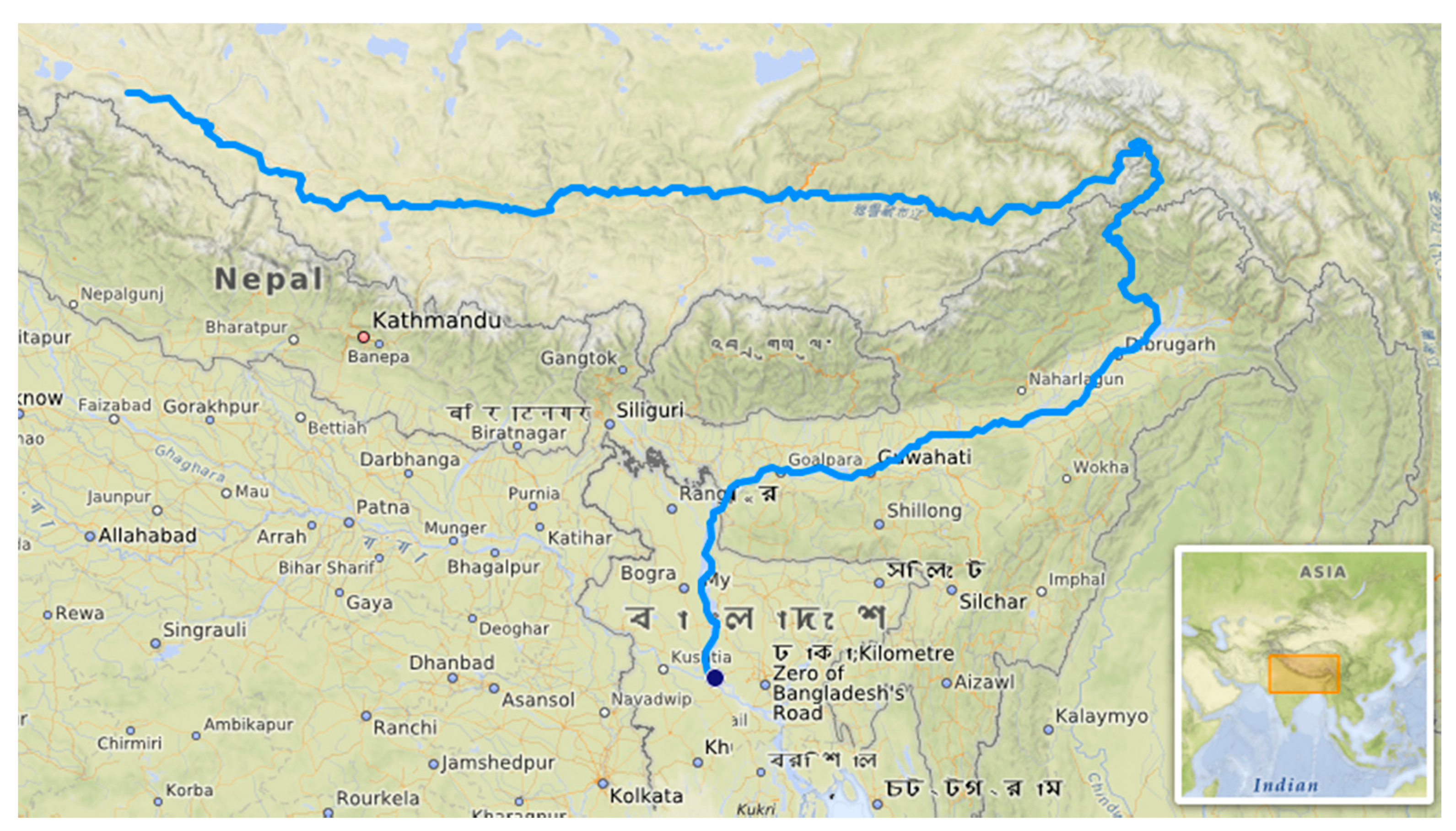
The Brahmaputra River (Figure 1), located in South Asia, situated between 23°N and 32°N latitude and 82°E and 97°E longitude is considered the fifth largest river system globally in terms of annual average discharges (about 20,000 m3/s) [72].
The basin has a maximum east-west length of 1540 km and north-south width of 682 km. On Indian territory, the Brahmaputra valley is narrow and long, has 640 km length and 64–90 km width [73]. The Brahmaputra basin covers 580,000 km2 in India, China, Bangladesh, and Bhutan [74]. It flows into the Bay of Bengal after joining with Ganga. The main canal of the Brahmaputra River crosses China, India, and Bangladesh and is2880 km in length. Three zones of the river basin can be distinguished: the Tibetan Plateau (TP) (with an elevation between 3000 and 5000 m), the Himalayan Belt (with elevations between 100 m and 3500 m), and the floodplain [72].
In the basin area, there are four seasons: the relatively dry-cool, dry-hot, the southwest monsoon, and retreating monsoon during December–February, March–May, June–September, and October–November, respectively.
Climatic conditions influence the annual regime of river flow. On the Indian Territory, the River has 11 main tributaries [75] that experience two high-water seasons, so the agricultural sector suffers from frequent flooding.
The flood’s consequence is a large-scale persistent erosion of the river’s banks. During the rainy season, it causes the breakage of the banks that are not robust enough to cope with the high pressure of the overflowing waters. Silt and sandy materials are carried by waters, affecting the cultivated agricultural lands that become unsuitable for immediate use. Generally, flooding happens during the monsoon season. Several floods have devastated the lands situated in the Brahmaputra basin in the last decades [76].
The yearly sediment load is about 735,000,000 metric tons, while its specific flood discharge is 0.15 m3/s/km2.
The soils in the Brahmaputra basin are Lithosols (in the Tibetan Plateau), orthic acrisols (in the Himalayan belt), and eutric cambisols and eutric gleysols (in the floodplain) [76].
The potentially usable water resources are estimated at 50 km3/year, out of which about 90% remain unutilized. The river’s waters are mainly utilized for irrigation (81%), household use (10%), and in the food (9%) industry [77].
Data series were downloaded from the site of ENVIS Centre on Control of Pollution Water, Air, and Noise [78]. They are data from official reports of the Ministry of Environment and Forests from India and contain the annual series of temperature (°C), pH, BOD (mg/L), DO (mg/L), electrical conductivity (EC) (µmhos/cm), Nitrate and Nitrite (mg/L), (fecal coliform (FC) (MPM/100 mL), and total coliform (TC) (MPM/100 mL) collected from 2003 to 2019 at ten hydrological stations (denoted in the following by S1–S10) situated on the Brahmaputra River.
2.2. Preliminary Statistical Analyses
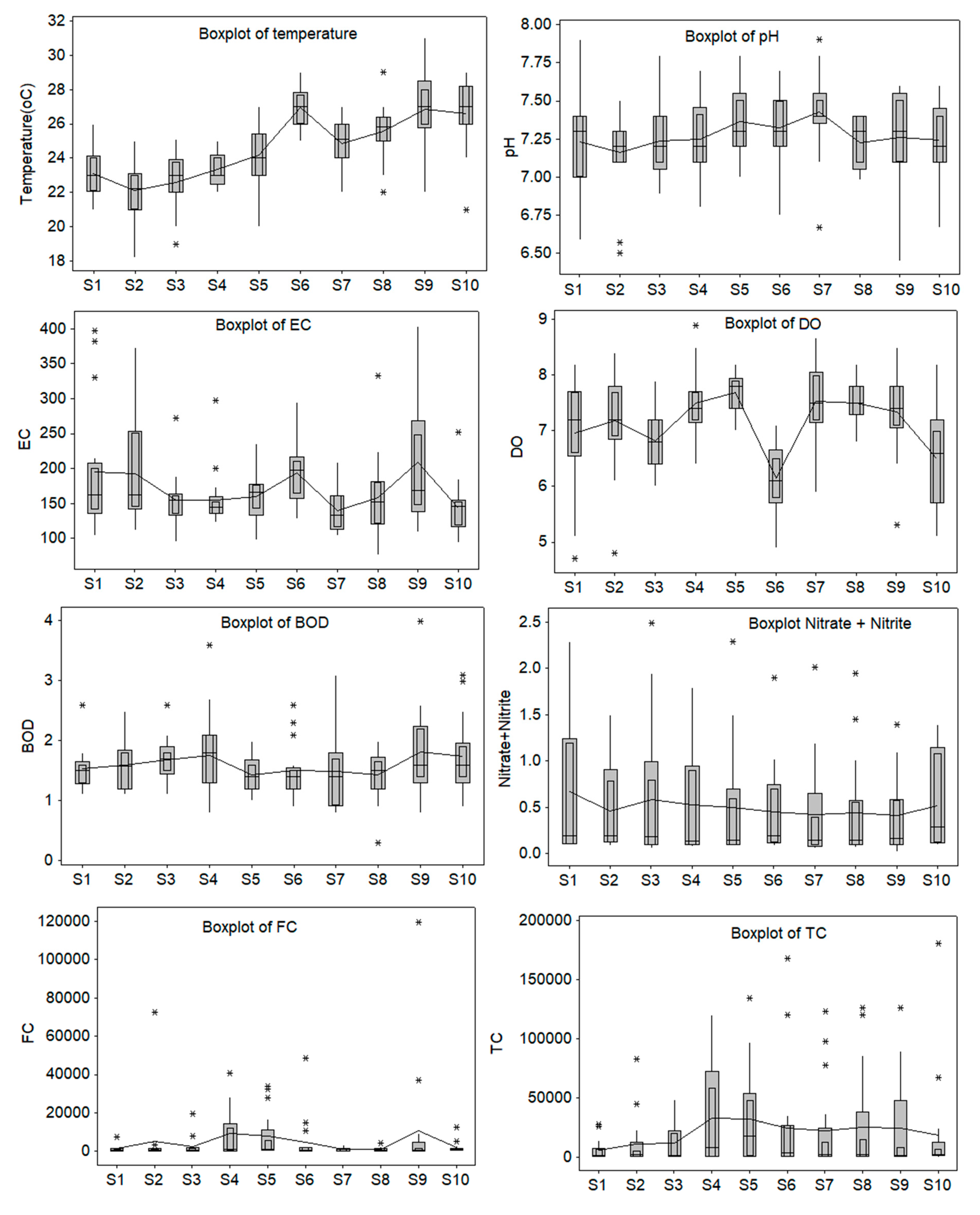
The boxplots for the water parameters were drawn to detect the series variability and the outliers’ existence.
To verify the hypothesis that there is no trend against the existence of a monotonic trend of a particular series of water parameters, the Mann–Kendall trend test [79] was used, followed by the nonparametric procedure of Sen [80] if the null hypothesis was been rejected.
The Kruskal–Wallis test was performed to determine if the series of a specific pollutant recorded at different sites come from the same distribution [81].
A loess trend was built to emphasize the evolution of each series of water parameters over the entire study period. In this procedure, for fitting the values at a point, the values from its neighbors are utilized weighted by the distance between the target point and the neighbor. A parameter α controls the size of the neighborhood. For α < 1, the neighborhood includes a proportion α of the points, with tricubic weighting [82]. In this analysis, α was chosen 0.10, 0.25, and 0.50, for comparison reasons.
2.3. The Water Pollution Indices
Three water quality indexes were computed to evaluate the water pollution at each station and the yearly pollution along the river. They are the Canadian Council Water Quality Index (CCME WQI) [83], the British Columbia Water Quality Index (BC WQI) [84], and the arithmetic weighted index [39]. These indexes are defined in the following.
CCME WQI is computed by:
where
- (a)
- F1 is the ratio between the number of the failed parameters and the total number of parameters, multiplied by 100;
- (b)
- F2 is the ratio between the number of the failed tests and the total number of tests, multiplied by 100.
An individual excursion is computed by:
If a test value falls below the objective value, and:
If a test value exceeds the objective value.
BC WQI is defined by [81]:
where
F1 = number of objectives not met/total number of objectives × 100, F2 = frequency of objectives not met/all instances of the objectives × 100, F3 = maximum deviation from any objectives.
Based on the CCME WQI, the following classes of water quality are determined: 95–100, Excellent; 80–94, Good; 65–79, Fair; 45–64, Marginal; and 0–44, Poor.
Based on the CCME WQI, the water categories are 0–3, Excellent; 4–17, Good; 18–43, Fair; 44–59, Borderline; 60–100, Poor.
The arithmetic weighted index [39] is defined by:
where wi is the weight corresponding to the quality index associated to the ith parameter,
V0 =7.0 for the pH, V0 = 14.6 mg/L for DO, and V0 = 0 for the other water parameters, Vi is the concentration of ith water parameter, Si is the standard value of the ith parameter and:
The water quality is Excellent, Good, Poor, Very Poor, or Unsuitable for drinking if the weighted arithmetic index is in the ranges (0–25), (26–50), (51–75), (76–100), and (above 100), respectively.
2.4. Classification
The sets of the WQIs computed at the previous stage were utilized to group the stations (respectively, the yearly series) in different clusters using agglomerative hierarchical clustering [85]. The optimal number of clusters was determined based on the majority principle after running 28 selection algorithms implemented in the NbClust package in R software [86].
2.5. Determination of the WQI Trend in Time and over the Region
The following procedure was utilized to determine the regional trend of the WQIs. This is a version of Method II from [25], where the k-mean clustering is replaced by the hierarchical clustering.
Suppose that k data series registered in n consecutive periods are provided and let us denote by (yji) (j = 1, …, n) the series registered at the station i (i = 1, …, m).
(II1) Choose the number of clusters and perform the clustering;
(II2) Determine the cluster containing the highest number of elements and build a matrix using the data series recorded at the sites from that cluster;
(II3) Choose the value representing the row j to be the average of the values recorded at the moment j at the stations from the cluster with the highest number of observations;
(II4) Represent graphically the results;
(II5) Compute the mean absolute error (MAE) and Mean Standard Error (MSE) and mean absolute percentage error (MAPE) corresponding to all the observation sites to assess the goodness-of-fit of the regional series.
The same procedure is applied for assessing the temporal trend of the WQI. In this case, the involved matrix (yji)’ is the transposed of (yji) from the above algorithm, so the sites are replaced by the periods and vice-versa.
In both cases, the procedure is applied for the WQIs yearly computed by the weighted index.
3. Results and Discussion
3.1. Statistical Analysis
Figure 2 displays the boxplots of the study parameters recorded at the stations S1-S10. All series present outliers. Notice the high values recorded for TC and FC at S5-S10, and FC at S9, S2, S6, and S5. Some extreme values of EC are present at S1 and for BOD at S9, S10, and S10. Thus, these values negatively impact the WQI.
After performing the Mann–Kendall test, the null hypothesis was rejected for most series. Table 1 contains the results of Sen’s slope estimation for the water parameters series registered at the hydrological stations. The positive values indicate an increasing trend; the negative ones point out a decreasing trend, whereas ‘-’ means that the null hypothesis cannot be rejected.
Table 1 shows that the series of nitrate and nitrites have an increasing trend at all the stations, while the EC trend is decreasing at six out of ten sites. The TC series does not present a trend. FC has an accentuated negative slope at S1 and a small one at S8. Overall, the highest variability of the water parameters is noticed at S1, followed by S8.
The Kruskal–Wallis test applied to the series of the same parameter collected at different stations rejected the null hypothesis only for temperature, EC, and DO.
Only a few series present a trend: temperature in 2008, 2009, 2011–2014, 2016–2019, EC in 2006 and 2010, and FC in 2018. There is only one series with a negative trend, EC (in 2006). So, the spatial variability is more accentuated than the temporal one. Taking into account these results, one might expect slight variations in the values of water quality indicators.
The Kruskal–Wallis test applied to the annual series of parameters rejected the null hypothesis for all water parameters but temperature and DO. This means that significant differences among the annual evolution of the water parameters were found.
Table 2 presents the slope evaluation for the yearly series for which the null hypothesis of the Mann–Kendall test was rejected.
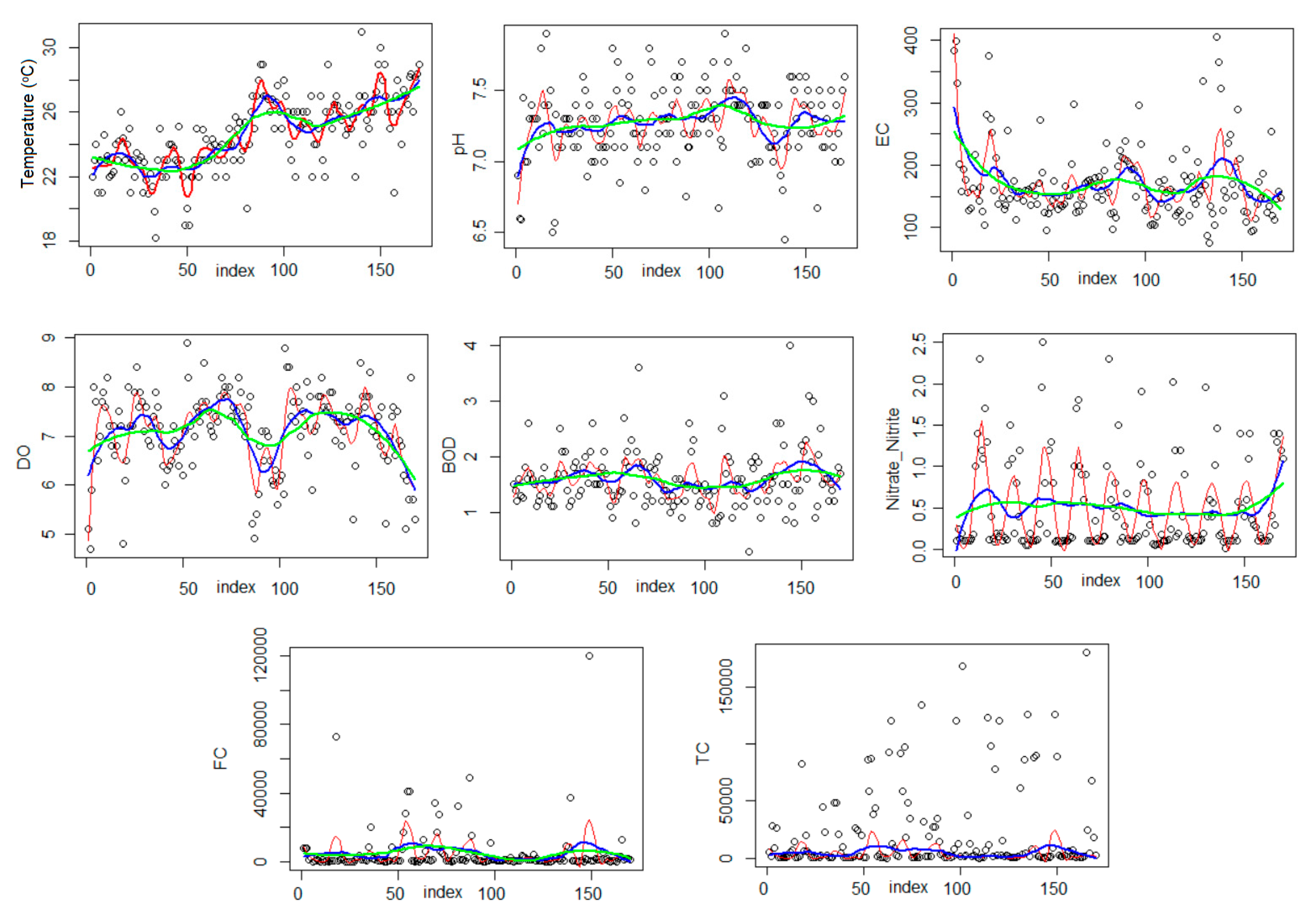
To have a complete image of the spatial and temporal variation in the water parameters, the loess curve was fitted for each series, with different values of the parameter α. The blue curve in Figure 3 corresponds to α = 0.10, the blue one to α = 0.25, and the green one to α = 0.50.
The loess curves for α = 0.10, (red) presents a periodical behavior for almost all series, with the highest variation for DO and Nitrate and Nitrite. Compared with the other loess curves (green and blue), their amplitudes are higher. This means that the influence of pollution in the locations closer to the analyzed site is more significant than the influence of the concentrations recorded at longer distances.
Figure 3 shows that the pollution is not uniformly distributed along the river, and overall, the pollution did not decrease during the study period.
3.2. WQIs Computation
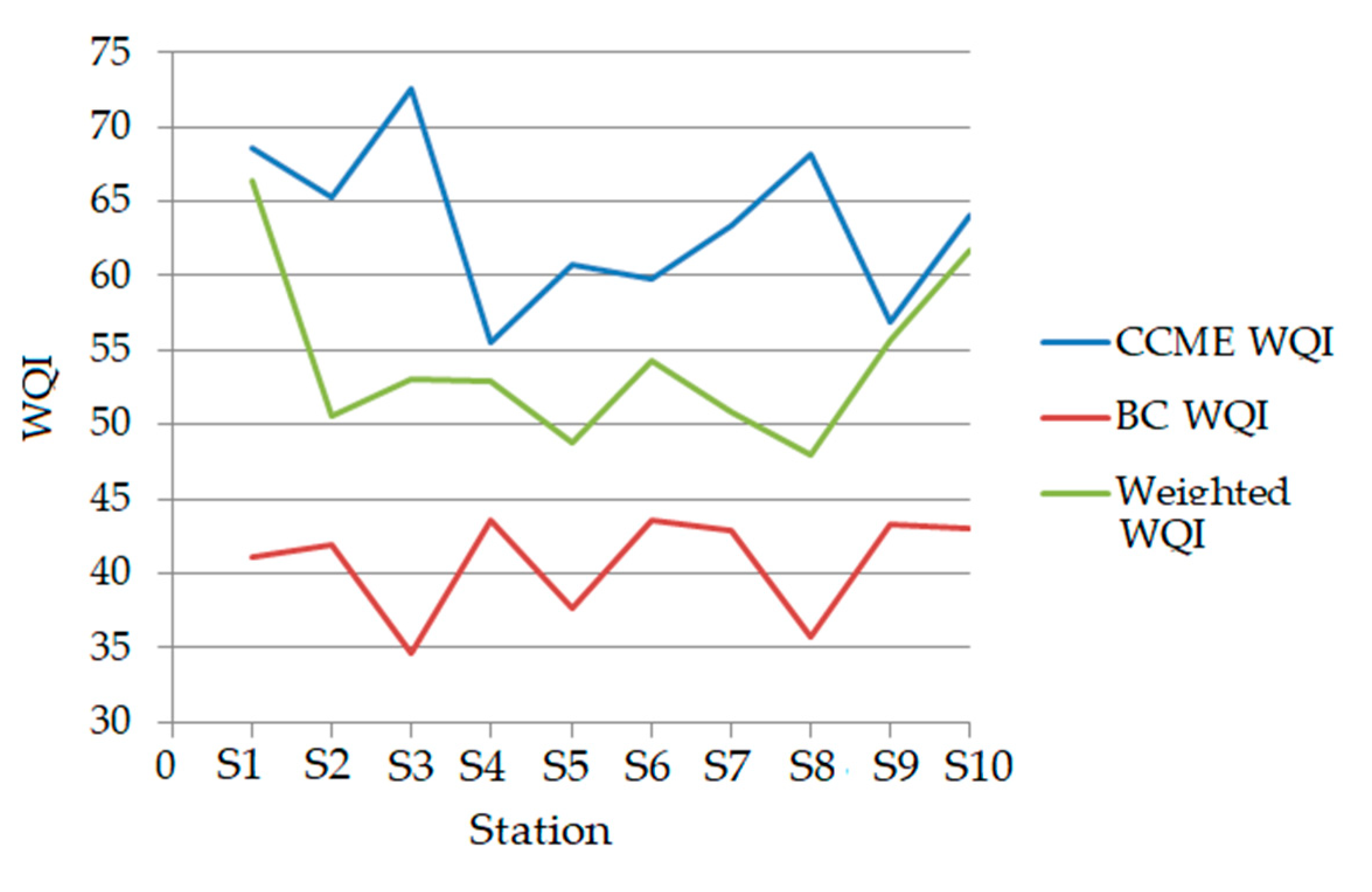
The values of the water quality indicators computed at the hydrological stations are presented in Figure 4. Table 3 contains the waters’ classification based on the calculated indexes.
Based on the CCME WQI, all but the water samples are classified as marginal or fair. Based on the BC WQI, they are fair or fair to borderline, whereas the water quality falls in the categories, poor or good, based on the weighted index.
3.3. Clustering Data Series
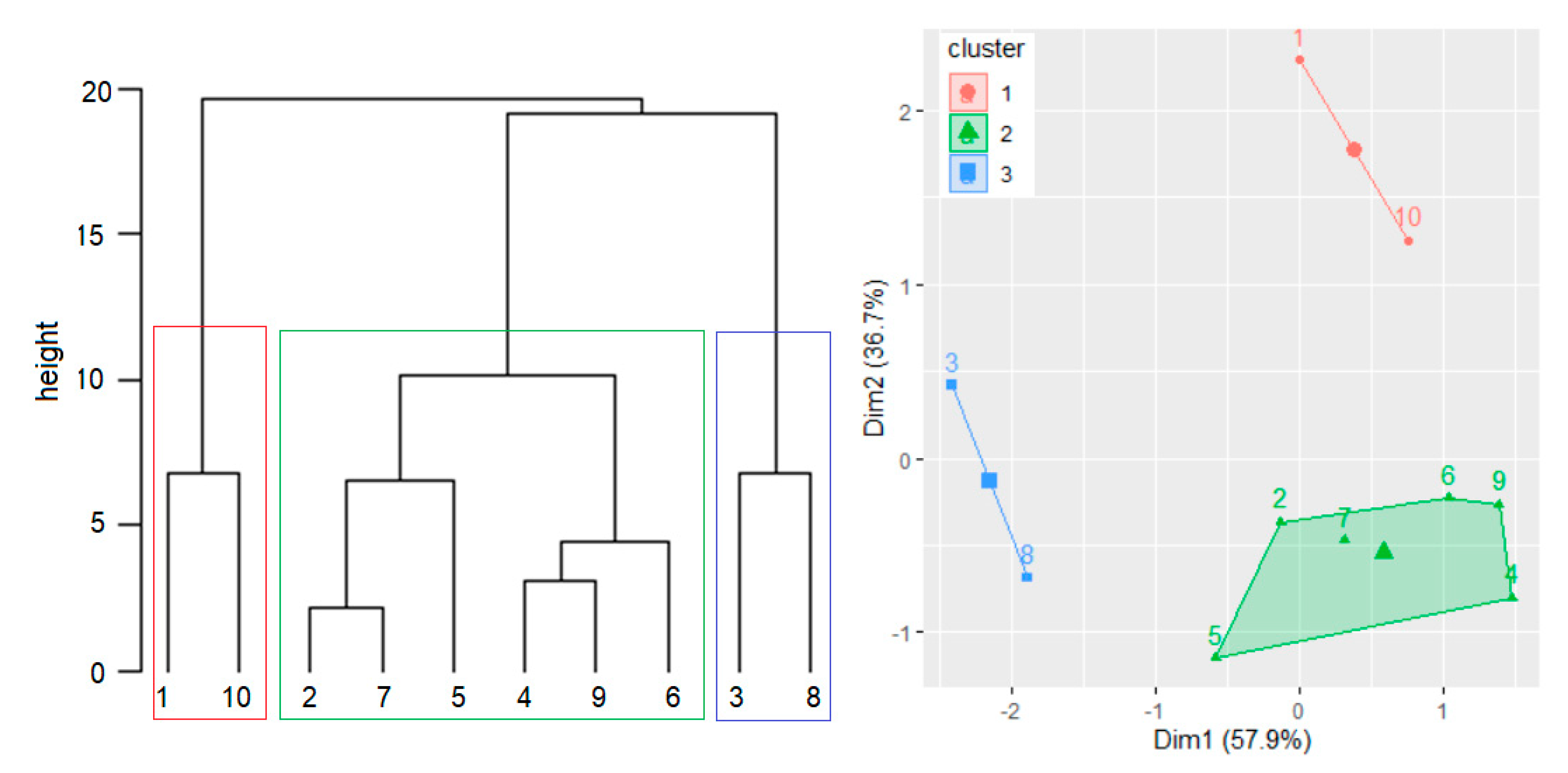
In the hierarchical clustering performed after scaling the WQIs from Table 3, three clusters were utilized. This number was determined by running 28 algorithms, among which ten selected three as the optimal value of the numbers of groups. The corresponding agglomerative coefficient was 0.755. Figure 6 displays the dendrogram and the clusters obtained.
The first and third clusters contain only two stations, whereas the second one has six elements. The four variables utilized to build CCME WQI do not meet the objectives for S1 and S10.
The null hypothesis could not be rejected by the Kruskal–Wallis test for the average value of the eight water parameters registered at S1 and S10. The same is true for the series in the other two clusters, confirming the correct clustering.
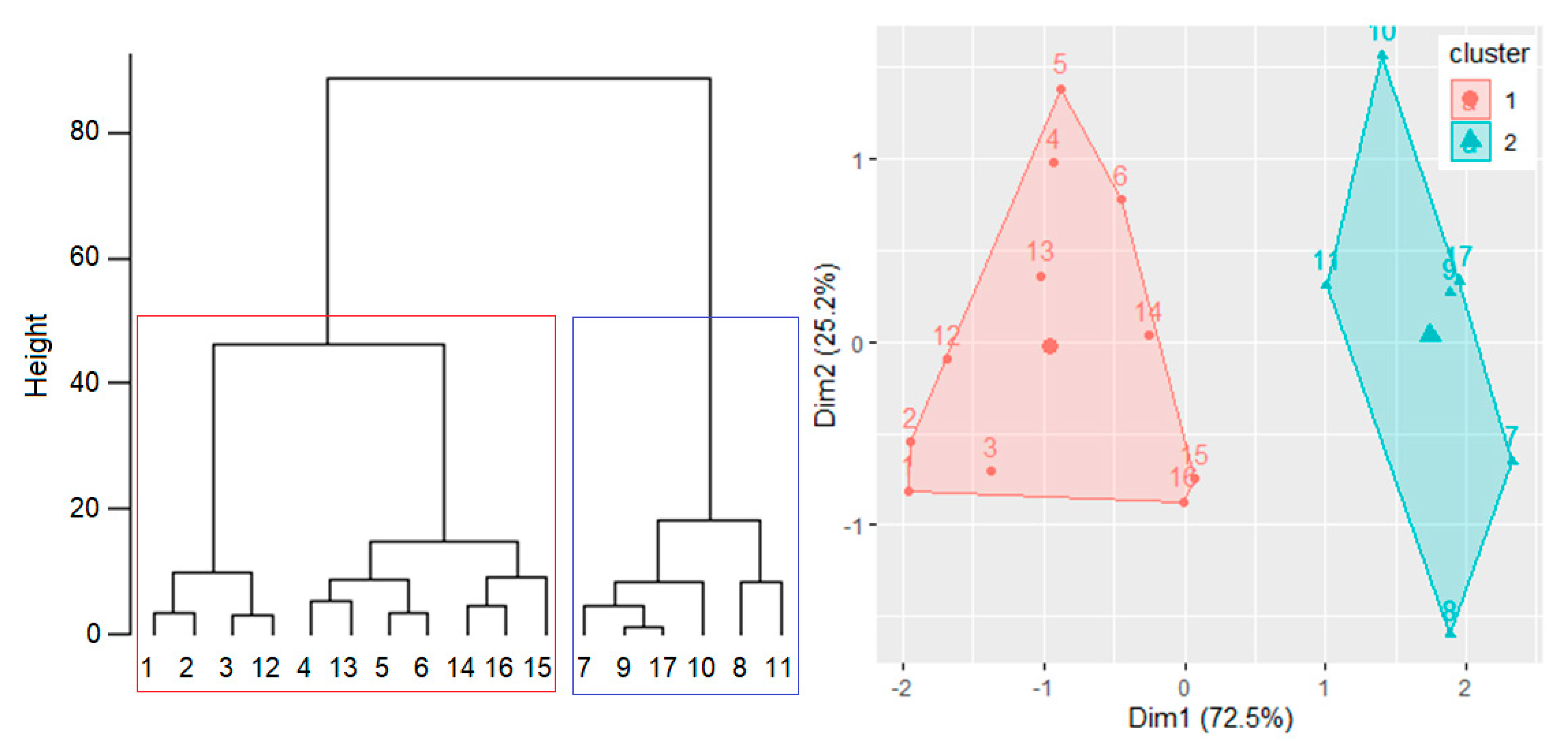
Hierarchical clustering was performed (after scaling the computed WQIs) using two clusters because 10 out of the 28 methods performed for finding the optimal number of groups found this number (two groups).
For measuring the clustering amount, the agglomerative coefficient was computed as well. Since its value was 0.947, the clustering is good.
The dendrogram produced by the agglomerative algorithm and the clusters are presented in Figure 7.
The series contained in the second cluster are characterized by values of FC and TC under the admissible limits, CCME WQI good, and BC WQI, good or fair.
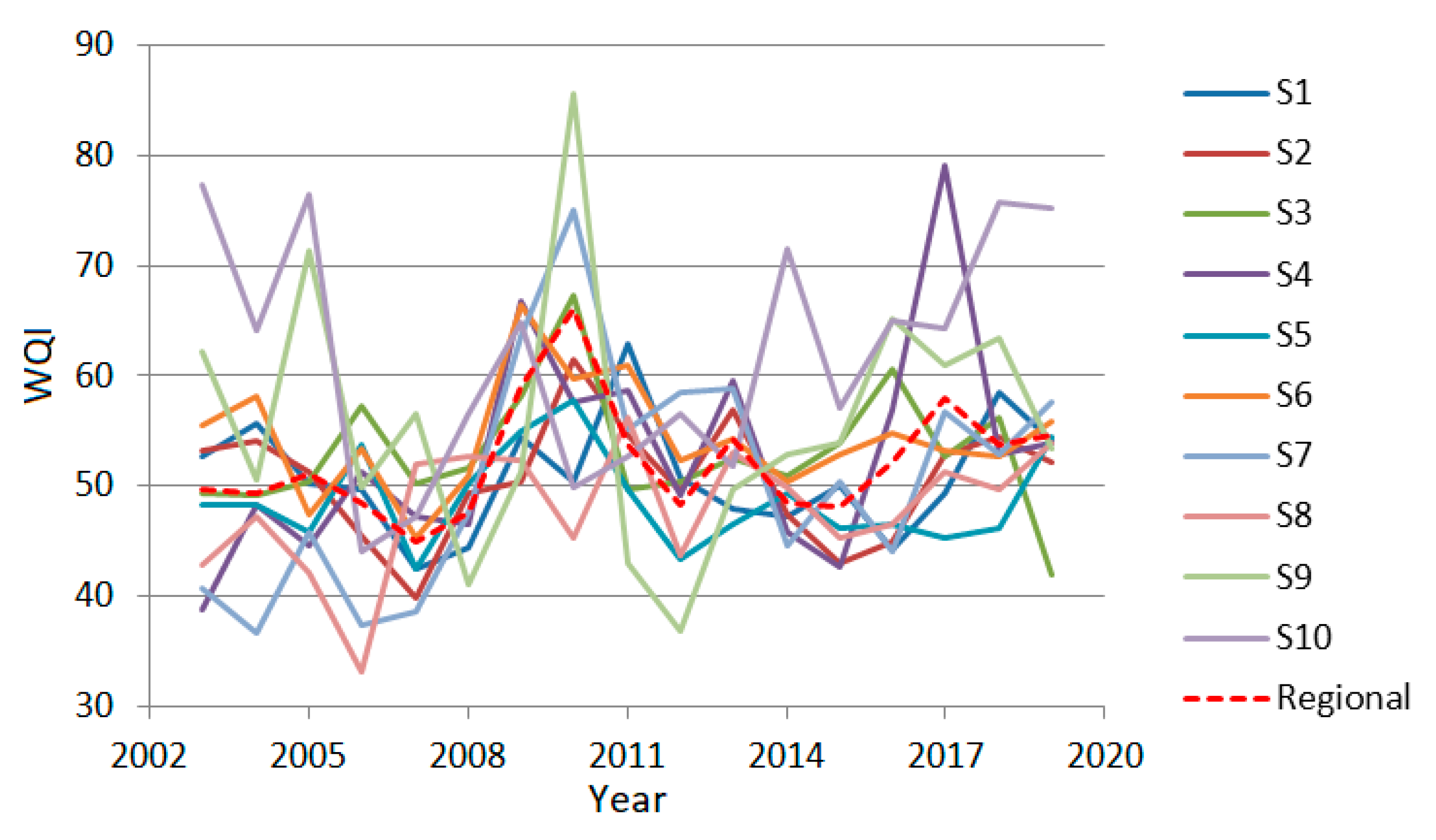
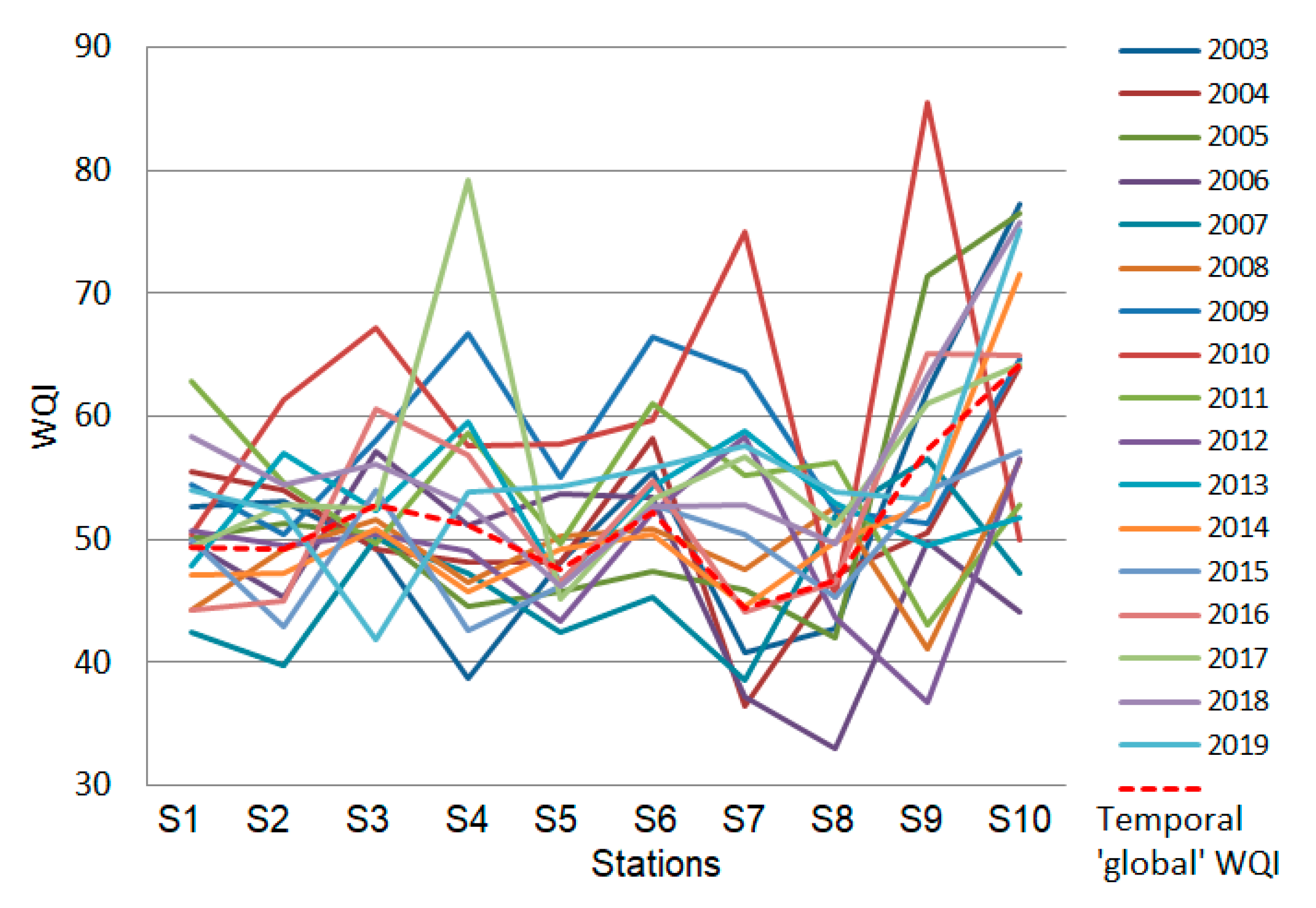
3.4. Determination of the Regional Series and Temporal ‘Global’ Series
The ‘regional’ series is the series that describes the WQI trend at the spatial scale. It is represented in Figure 8 by the red line and was computed as described in the first part of Section 2.5. The goodness of fit indicators are provided in Table 5.
All the MAE, RMSE, and MAPE values are small, showing a good fitting of the regional trend of WQIs. The MAPE values are the smallest. Since MAPE is not a dimensional indicator, it is most suitable for assessing the modeling quality.
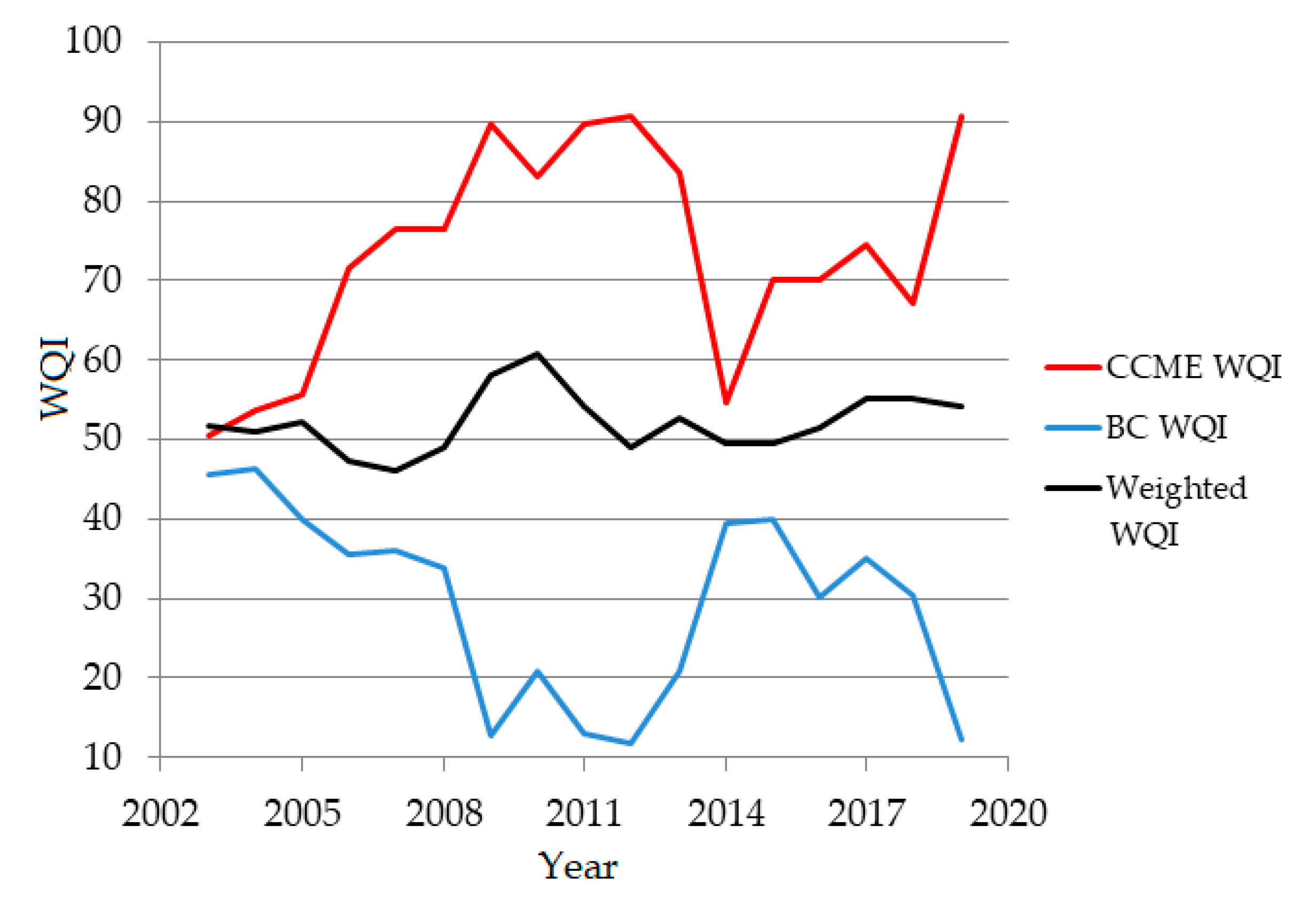
The temporal ’global’ series is the series that describes the WQI evolution in time, computed as presented in the second part of Section 2.5. It is represented in Figure 9 by the red line. The goodness of fit indicators are provided in Table 6.
In Table 6, MAEs are under 12.60, RMSE under 15.77, and MAPE under 2.14, indicating a good fit of the temporal ‘global’ series. The lowest fit quality is noticed for 2011, in terms of MAPE, and 2010, in terms of MAE and MSE. These are due to a better quality (higher QWI) recorded at the stations S1 and S9, respectively.
3.5. Discussions of the Present Results Compared with Previous Research
The above results showed that the quality of the Brahmaputra River is not very good. There is a concordance of the water quality classification based on all the used indexes. The results would be more precise if other water parameters were available and taken into account.
Still, our findings do not differ from those of other researchers. For example, Muyen et al. [87] analyzed the pollution of the Brahmaputra River in a sector from Bangladesh in April 2015, and found that the water is highly polluted. Kotoky and Sharma [88] confirmed this idea in a study performed in India in March 2017. They included the water to be in class IV (based on the used WQI). Mech and Hazarika [89] emphasized the impact of industrial effluents on the ecosystem and population lives near Brahmaputra Cracker. Tsering et al. [90] showed that the level of pollution of Brahmaputra with microplastics was extremely high in 2018–2019. The official report on the water quality scenario of rivers [91] emphasizes the increase in water turbidity during 2006–2019. The United Nations, through the Environment Program [92], drew a signal of alarm on the accelerated consequences of the Brahmaputra River’s pollution.
4. Conclusions
WQIs are mainly used to assess water quality over a long period and as a tool for making informed decisions on water management policy in water scarcity conditions. Even if there is no mathematical formula to estimate the risk of water consumption based on WQIs, a high WQI class means low risk for the population that consumes the water. For example, when working with the weighted index, if the water is classified as excellent or good, there is no risk for population’s health by its consumption.
Regulations establish allowable limits of water parameters. Since different water parameters can sometimes have values outside the permissible limits, these values should be observed. For example, high values of coliforms may result in diseases after water consumption. Therefore, the WQI use should be correlated with observation of the water parameters.
Other indicators are utilized to assess water use suitability for other purposes, such as agriculture. The series of Na, Cl, bicarbonate ions, Mg, Mn phosphates, and TDS concentrations are necessary to compute such indicators. Unfortunately, these data are not available on the official site [78] from where the other series were downloaded, which would permit us to perform the study in this direction. Still, an integrated analysis of water parameters and WQIs is the best approach for deciding water use for different activities.
This research investigated the series of eight water parameters recorded for 17 years to assess the water quality at the spatial and temporal scales. Based on the CCME WQI, the water quality was Fair (at S1, S2, S3, and S8) and Marginal (the other stations). Based on the BC WQI, the water was classified as Fair or Fair/Borderline. Based on the weighted index, the water was classified as either Poor or Good. The values of the WQIs computed for the annual series indicate a water quality decrease after 2015.
Two clusters were detected based on the computed WQIs for the annual series and three groups for the WQI series corresponding to the hydrological stations, employed to evaluate the WQI trend at the temporal and spatial scales. The water quality is mainly affected by the high concentrations of coliform that exceed many times the legal limits at some stations during the period 2003–2019.
This approach combined the statistical analysis, the computation of the water quality indicators, classification, and trend modeling to evaluate the water quality of the Brahmaputra River. We intend to extend the research by involving more water indicators and other techniques to assess water quality better.
Author Contributions
Conceptualization, A.B. and C.S.D.; methodology, A.B and C.S.D.; software, A.B; validation, C.S.D.; formal analysis, L.B.; investigation, A.B. and L.B.; resources, L.B.; data curation, A.B. and C.S.D.; writing—original draft preparation, A.B. and L.B.; writing—review and editing, A.B. and C.S.D.; visualization, A.B.; supervision, A.B.; project administration, A.B.; funding acquisition, L.B. All authors have read and agreed to the published version of the manuscript.
Funding
This research received no external funding.
Institutional Review Board Statement
Not applicable.
Informed Consent Statement
Not applicable.
Data Availability Statement
Conflicts of Interest
The present research works carry no conflict of interest.
References
- Singh, A.; Sharam, R.K.; Agrawal, M.; Marshall, F.M. Health risk assessment of heavy metals via dietary intake of foodstuffs from the wastewater irrigated site of a dry tropical area of India. Food Chem. Toxicol. 2010, 48, 611–619. [Google Scholar] [CrossRef]
- U.S. Environmental Protection Agency (EPA). Ecological Risk Models and Tools. 2021. Available online: https://www.epa.gov/risk/ecological-risk-models-and-tools (accessed on 20 September 2021).
- Avigliano, E.; Schenone, N.F. Human health risk assessment and environmental distribution of trace elements, glyphosate, fecal coliform and total coliform in Atlantic Rainforest mountain rivers (South America). Microchem. J. 2015, 122, 149–158. [Google Scholar] [CrossRef]
- Mekuria, D.M.; Kassegne, A.B.; Asfaw, S.L. Assessing pollution profiles along Little Akaki River receiving municipal and industrial wastewaters, Central Ethiopia: Implications for environmental and public health safety. Heliyon 2021, 7, e07526. [Google Scholar] [CrossRef]
- Bărbulescu, A.; Maftei, C.; Dumitriu, C.S. The modelling of the climateric process that participates at the sizing of an irrigation system. Bull. Appl. Comput. Math. 2002, 2048, 11–20. [Google Scholar]
- Nambatingar, N.; Clement, Y.; Merle, A.; New Mahamat, T.; Lanteri, P. Heavy metal pollution of Chari river water during the crossing of N’Djamena (Chad). Toxics 2017, 5, 26. [Google Scholar] [CrossRef]
- Zhou, T.; Wu, J.; Peng, S. Assessing the effects of landscape pattern on river water quality at multiple scales: A case study of the Dongjiang River watershed, China. Ecol. Indic. 2012, 23, 166–175. [Google Scholar] [CrossRef]
- Campanale, C.; Dierkes, G.; Massarelli, C.; Bagnuolo, G.; Uricchio, V.F. A relevant screening of organic contaminants present on freshwater and pre-production microplastics. Toxics 2020, 8, 100. [Google Scholar] [CrossRef] [PubMed]
- Al-Taani, A.; Nazzal, Y.; Howari, F.; Iqbal, J.; Bou-Orm, N.; Xavier, C.M.; Bărbulescu, A.; Sharma, M.; Dumitriu, C.S. Contamination assessment of heavy metals in soil, Liwa area, UAE. Toxics 2021, 9, 53. [Google Scholar] [CrossRef] [PubMed]
- Mihăilescu, M.; Negrea, A.; Ciopec, M.; Negrea, P.; Duțeanu, N.; Grozav, I.; Svera, P.; Vancea, C.; Bărbulescu, A.; Dumitriu, C.S. Full factorial design for gold recovery from industrial solutions. Toxics 2021, 9, 111. [Google Scholar] [CrossRef]
- Nazzal, Y.H.; Bărbulescu, A.; Howari, F.; Al-Taani, A.A.; Iqbal, J.; Xavier, C.M.; Sharma, M. Dumitriu, C.Ș. Assessment of metals concentrations in soils of Abu Dhabi Emirate using pollution indices and multivariate statistics. Toxics 2021, 9, 95. [Google Scholar] [CrossRef] [PubMed]
- Pisciotta, J.M.; Rath, D.F.; Stanek, P.A.; Flanery, D.M.; Harwood, V.J. Marine bacteria cause false-positive results in the colilert-18 rapid identification test for escherichia coli in florida waters. Appl. Environ. Microbiol. 2002, 68, 539–544. [Google Scholar] [CrossRef] [PubMed] [Green Version]
- Seo, M.; Lee, H.; Kim, Y. Relationship between coliform bacteria and water quality factors at weir stations in the Nakdong River, South Korea. Water 2019, 11, 1171. [Google Scholar] [CrossRef] [Green Version]
- Aonofriesei, F.; Bărbulescu, A.; Dumitriu, C.-S. Statistical analysis of morphological parameters of microbial aggregates in the activated sludge from a wastewater treatment plant for improving its performances. Rom. J. Phys. 2021, 66, 809. [Google Scholar]
- Vadde, K.K.; Jianjun, W.; Long, C.; Tianma, Y.; Alan, J.; Raju, S. Assessment of water quality and identification of pollution rick locations in Tiaoxi River (Taihu watershed), China. Water 2017, 10, 183. [Google Scholar] [CrossRef] [Green Version]
- Xu, H.; Paerl, H.W.; Qin, B.; Zhu, G.; Gaoa, G. Nitrogen and phosphorus inputs control phytoplankton growth in eutrophic Lake Taihu, China. Limnol. Oceanogr. 2010, 55, 420–432. [Google Scholar] [CrossRef] [Green Version]
- Gupta, S.; Gupta, S.K. A critical review on water quality index tool: Genesis, evolution and future directions. Ecol. Inform. 2021, 63, 101299. [Google Scholar] [CrossRef]
- Bărbulescu, A. Assessing groundwater vulnerability: DRASTIC and DRASTIC-like methods: A review. Water 2020, 12, 1356. [Google Scholar] [CrossRef]
- Bărbulescu, A.; Dumitriu, C.Ș. Assessing the water quality by statistical methods. Water 2021, 13, 1026. [Google Scholar] [CrossRef]
- Bărbulescu, A.; Barbeş, L. Assessing the water quality of the Danube River (at Chiciu, Romania) by statistical methods. Environ. Earth Sci. 2020, 79, 122. [Google Scholar] [CrossRef]
- Razmkhah, H.; Abrishamchi, A.; Torkian, A. Evaluation of spatial and temporal variation in water quality by pattern recognition techniques: A case study on jajrood river (Tehran, Iran). J. Environ. Manag. 2010, 91, 852–860. [Google Scholar] [CrossRef]
- Ogwueleka, T.C. Use of multivariate statistical techniques for the evaluation of temporal and spatial variations in water quality of the Kaduna River, Nigeria. Environ. Monit. Assess. 2015, 187, 137. [Google Scholar] [CrossRef]
- Sheikhy Narany, T.; Ramli, M.F.; Aris, A.Z.; Sulaiman, W.N.; Fakharian, K. Spatiotemporal variation of groundwater quality using integrated multivariate statistical and geostatistical approaches in Amol-Babol Plain. Iran. Environ. Monit. Assess. 2014, 186, 5797–5815. [Google Scholar] [CrossRef] [PubMed]
- Sharma, A.; Bora, C.R.; Shukla, V. Evaluation of seasonal changes in physico-chemical and bacteriological characteristics of water from the Narmada River (India) using multivariate analysis. Nat. Resour. Res. 2013, 22, 283–296. [Google Scholar] [CrossRef]
- Bărbulescu, A.; Postolache, F.; Dumitriu, C.Ș. Estimating the precipitation amount at regional scale using a new tool, Climate Analyzer. Hidrology 2021, 8, 125. [Google Scholar] [CrossRef]
- Dragomir, F.L. Modeling and Simulation of the Systems and Processes; Editura Universității Naționale de Apărare Carol I: București, Romania, 2017. (In Romanian) [Google Scholar]
- Dragomir, F.L. Decision Theory—Theoretical Notions; Editura Universității Naționale de Apărare Carol I: București, Romania, 2017. (In Romanian) [Google Scholar]
- Dragomir, F.L. Operational Research; Editura Universității Naționale de Apărare Carol I: București, Romania, 2017. (In Romanian) [Google Scholar]
- Tiyasha, S.; Tung, T.M.; Yaseen, Z.M. A survey on river water quality modelling using artificial intelligence models: 2000–2020. J. Hydrol. 2020, 585, 124670. [Google Scholar] [CrossRef]
- Jiang, Y.; Nan, Z.; Yang, S. Risk assessment of water quality using Monte Carlo simulation and artificial neural network method. J. Environ. Manag. 2013, 122, 130–136. [Google Scholar] [CrossRef]
- Divya, A.H.; Soloman, P.A. Assessment of river water quality indices based on various fuzzy models and arithmetic indexing method. IOP Conf. Ser. Mater. Sci. Eng. 2021, 1114, 012092. [Google Scholar] [CrossRef]
- Landwehr, J.M. A statistic view of a class of water quality indices. Water Resour. Res. 1979, 15, 460–468. [Google Scholar] [CrossRef]
- House, M.A.; Newsome, D.H. Water quality indices for the management of surface water quality. Water Sci. Technol. 1989, 21, 1137–1148. [Google Scholar] [CrossRef]
- Horton, R.K. An index number system for rating water quality. J. Wat. Pollut. Con. Fed. 1965, 37, 300–305. [Google Scholar]
- Uddin, M.G.; Nash, S.; Olbert, A.I. A review of water quality index models and their use for assessing surface water quality. Ecol. Indic. 2021, 122, 107218. [Google Scholar] [CrossRef]
- Bascaron, M. Establishment of a methodology for the determination of water quality. Bull. Inform. Medio Amb. 1979, 9, 30–51. [Google Scholar]
- CCME, Canadian Water Quality Index 1.0. Technical Report and User’s Manual Gatineau, QC: Canadian Council of Minister of the Environment, Canadian Environmental Quality Guidelines, Water Quality Index Technical Subcommittee. 2021. Available online: http://ceqg-rcqe.ccme.ca/download/en/138 (accessed on 15 August 2020).
- Dinius, S.H. Design of an Index of Water Quality. J. Am. Water Resour. Assoc. 1987, 23, 833–843. [Google Scholar] [CrossRef]
- Cude, C.G. Oregon water quality index: A tool for evaluating water quality management effectiveness. J. Am. Water Resour. Assoc. 2001, 37, 125–137. [Google Scholar] [CrossRef]
- Sutadian, A.D.; Muttil, N.; Yilmaz, A.G.; Perera, B.J.C. Development of a water quality index for rivers in West Java Province, Indonesia. Ecol. Indic. 2018, 85, 966–982. [Google Scholar] [CrossRef]
- Gupta, A.K.; Gupta, S.K.; Patil, R.S. A comparison of water quality indices for coastal water. J. Environ. Sci. Health Part A 2003, 38, 2711–2725. [Google Scholar] [CrossRef]
- Almeida, C.; Gonzalez, S.O.; Mallea, M.; Gonzalez, P. A recreational water quality index using chemical, physical and microbiological parameters. Environ. Sci. Pollut. Res. 2012, 19, 3400–3411. [Google Scholar] [CrossRef]
- Dojlido, J.A.N.; Raniszewski, J.; Woyciechowska, J. Water quality index applied to rivers in the Vistula River basin in Poland. Environ. Monit. Assess. 1994, 33, 33–42. [Google Scholar] [CrossRef]
- Liou, S.-M.; Lo, S.-L.; Wang, S.-H. A Generalized Water Quality Index for Taiwan. Environ. Monit. Assess. 2004, 96, 35–52. [Google Scholar] [CrossRef]
- MacDonald, D.D.; Berger, T.; Wood, K.; Brown, J.; Johnsen, T.; Haines, M.L.; Brydges, K.; MacDonald, M.J.; Smith, S.L.; Shaw, D.P. A Compendium of Environmental Quality Benchmarks. Available online: https://www.lm.doe.gov/cercla/documents/rockyflats_docs/SW/SW-A-005694.pdf (accessed on 2 November 2021).
- Rocchini, R.; Swain., L.G. The British Columbia Water Quality Index; Water Quality Branch, Environmental Protection Department British Columbia Ministry of Environment, Lands and Parks: Victoria, BC, Canada, 1995; p. 13. [Google Scholar]
- Wright, C.R.; Saffran, K.A.; Anderson, A.-M.; Neilson, R.D.; MacAlpine, N.D.; Cooke, S.E. A Water Quality Index for Agricultural Streams in Alberta: The Alberta Agricultural Water Quality Index (AAWQI); Prepared for the Alberta Environmentally Sustainable Agriculture Program (AESA). Alberta Agriculture, Food and Rural Development: Edmonton, AB, Canada, 1999; p. 35. [Google Scholar]
- Granata, F.; Papirio, S.; Esposito, G.; Gargano, R.; de Marinis, G. Machine Learning Algorithms for the Forecasting of Wastewater Quality Indicators. Water 2017, 9, 105. [Google Scholar] [CrossRef] [Green Version]
- Oladipo, J.O.; Akinwumiju, A.S.; Aboyeji, O.S.; Adelodun, A.A. Comparison between fuzzy logic and water quality index methods: A case of water quality assessment in Ikare community, Southwestern Nigeria. Environ. Chall. 2021, 3, 100038. [Google Scholar] [CrossRef]
- Shah, M.I.; Alaloul, W.S.; Alqahtani, A.; Aldrees, A.; Musarat, M.A.; Javed, M.F. Predictive Modeling Approach for Surface Water Quality: Development and Comparison of Machine Learning Models. Sustainability 2021, 13, 7515. [Google Scholar] [CrossRef]
- Bărbulescu, A.; Nazzal, Y.; Howari, F. Assessing the groundwater quality in the Liwa area, the United Arab Emirates. Water 2020, 12, 2816. [Google Scholar] [CrossRef]
- Du, X.; Feng, J.; Fang, M.; Ye, X. Sources, Influencing Factors, and Pollution Process of Inorganic Nitrogen in Shallow Groundwater of a Typical Agricultural Area in Northeast China. Water 2020, 12, 3292. [Google Scholar] [CrossRef]
- Mamun, M.; Kim, J.Y.; An, K.-G. Multivariate Statistical Analysis of Water Quality and Trophic State in an Artificial Dam Reservoir. Water 2021, 13, 186. [Google Scholar] [CrossRef]
- Al-Taani, A.A.; Rashdan, M.; Nazzal, Y.; Howari, F.; Iqbal, J.; Al-Rawabdeh, A.; Al Bsoul, A.; Khashashneh, S. Evaluation of the Gulf of Aqaba Coastal Water, Jordan. Water 2020, 12, 2125. [Google Scholar] [CrossRef]
- Yu, Y.; Song, X.; Zhang, Y.; Zheng, F. Assessment of Water Quality Using Chemometrics and Multivariate Statistics: A Case Study in Chaobai River Replenished by Reclaimed Water, North China. Water 2020, 12, 2551. [Google Scholar] [CrossRef]
- Cui, L.; Wang, X.; Li, J.; Gao, X.; Zhang, J.; Liu, Z. Ecological and health risk assessments and water quality criteria of heavy metals in the Haihe River. Environ. Poll. 2021, 290, 117971. [Google Scholar] [CrossRef] [PubMed]
- Reitter, C.; Petzoldt, H.; Korth, H.; Schwab, F.; Stange, C.; Hambsch, B.; Tiehm, A.; Lagkouvardos, I.; Gescher, J.; Hügler, M. Seasonal dynamics in the number and composition of coliform bacteria in drinking water reservoirs. Sci. Total. Environ. 2021, 787, 147539. [Google Scholar] [CrossRef]
- Rising Problems and Solutions to Water Pollution in India. Available online: https://www.borgenmagazine.com/water-in-india/ (accessed on 25 July 2021).
- Water Pollution is Killing Millions of Indians. Here’s How Technology and Reliable Data Can Change That. Available online: https://www.weforum.org/agenda/2019/10/water-pollution-in-india-data-tech-solution/ (accessed on 25 July 2021).
- Pollution Assessment. River Ganga. Available online: https://cpcb.nic.in/wqm/pollution-assessment-ganga-2013.pdf (accessed on 25 July 2021).
- Avvannavar, S.M.; Shrihari, S. Evaluation of water quality index for drinking purposes for river Netravathi, Mangalore, South India. Environ. Monit. Assess. 2008, 143, 279–290. [Google Scholar] [CrossRef] [PubMed]
- Bhargava, D.S. Use of a water quality index for river classification and zoning of the Ganga River. Environ. Poll. 1983, B6, 51–67. [Google Scholar] [CrossRef]
- Rakhecha, P.R. Water environment pollution with its impact on human diseases in India. Int. J. Hydrol. 2020, 4, 152–158. [Google Scholar] [CrossRef]
- Bora, M.; Goswami, D.C. Water quality assessment in terms of water quality index (WQI): Case study of the Kolong River, Assam, India. Appl. Water Sci. 2017, 7, 3125–3135. [Google Scholar] [CrossRef] [Green Version]
- Bărbulescu, A.; Barbeş, L.; Dumitriu, C.Ş. Statistical assessment of the water quality using water quality indicators. A case study from India. In Water Safety and Security—Threat Detection and Mitigation, Advanced Sciences and Technologies for Security Applications; Vaseashta, A.K., Maftei, C., Eds.; Springer International Publishing AG: Cham, Switzerland, 2021; pp. 599–613. [Google Scholar]
- Bărbulescu, A.; Dani, A. Statistical analysis and classification of the water parameters of Beas River (India). Rom. Rep. Phys. 2019, 71, 716. [Google Scholar]
- Chakrabarty, S.; Sarma, H.P. A statistical approach to multivariate analysis of drinking water quality in Kamrup district, Assam, India. Arch. Appl. Sci. Res. 2011, 3, 258–264. [Google Scholar]
- Dimri, D.; Daverey, A.; Kumar, A.; Sharma, A. Monitoring water quality of River Ganga using multivariate techniques and WQI (Water Quality Index) in Western Himalayan region of Uttarakhand, India. Environ. Nanotechnol. Monit. Manag. 2021, 15, 100375. [Google Scholar]
- Singh, K.P.; Malik, A.; Sinha, S. Water quality assessment and apportionment of pollution sources of Gomti River (India) using, multivariate statistical techniques—A case study. Anal. Chem. Acta 2005, 538, 355–374. [Google Scholar] [CrossRef]
- Bhuyan, M.; Bakar, M.; Sharif, A.; Hasan, M.; Islam, M. Water quality assessment using water quality indicators and multivariate analyses of the Old Brahmaputra River. Pollution 2018, 4, 481–493. [Google Scholar]
- Gangwar, S. Water quality monitoring in India: A review. Int. J. Inform. Comput. Technol. 2013, 3, 851–856. [Google Scholar]
- Immerzeel, W. Historical trends and future predictions of climate variability in the Brahmaputra basin. Int. J. Climatol. 2008, 28, 243–254. [Google Scholar] [CrossRef]
- Datta, B.; Singh, V.P. Hydrology. In The Brahmaputra Basin Water Resources; Singh, V., Sharma, N., Ojha, C.S.P., Eds.; Kluwer Academic Publishers: New York, NY, USA, 2004; pp. 139–195. [Google Scholar]
- Purkait, B. Hydrometeorology. In The Brahmaputra Basin Water Resources; Singh, V., Sharma, N., Ojha, C.S.P., Eds.; Kluwer Academic Publishers: New York, NY, USA, 2004; Volume 47, pp. 24–34. [Google Scholar]
- Sarma, J.N. An overview of the Brahmaputra river system. In The Brahmaputra Basin Water Resources; Singh, V., Sharma, N., Ojha, C.S.P., Eds.; Kluwer Academic Publishers: New York, NY, USA, 2004; Volume 47, pp. 72–87. [Google Scholar]
- Mahanta, C.; Zaman, A.M.; Newaz, A.M.S.; Rahman, S.M.M.; MAzumdar, T.K.; Choudhury, R.; Borah, P.J.; Saikia, L. Physical assessment of the Brahmaputra River. In Ecosystems for Life: A Bangladesh-India Initiative; Prokashony, J., Ed.; International Union for Conservation of Nature: Dhaka, Bangladesh, 2014; p. 74. Available online: https://portals.iucn.org/library/node/45928 (accessed on 20 September 2021).
- Amarasinghe, U.A.; Sharma, B.R.; Aloysius, N.; Scott, C.; Smakhtin, V.; de Fraiture, C.; Shukla, A.K. Spatial Variation in Water Supply and Demand Across the River Basins of India; Research Report 83. International Water Management Institute: Colombo, Sri Lanka, 2004. Available online: https://www.iwmi.cgiar.org/publications/iwmi-research-reports/iwmi-research-report-83/ (accessed on 20 September 2021).
- ENVIS Centre on Control of Pollution Water, Air and Noise, Water Quality Database. Available online: http://www.cpcbenvis.nic.in/water_quality_data.html# (accessed on 15 September 2021).
- Kendall, M.G. Rank Correlation Methods, 4th ed.; Charles Griffin: London, UK, 1975. [Google Scholar]
- Sen, P.K. Estimates of the regression coefficient based on Kendall’s tau. J. Am. Stat. Assoc. 1968, 63, 1379–1389. [Google Scholar] [CrossRef]
- Corder, G.W.; Foreman, D.I. Nonparametric Statistics for Non-Statisticians; John Wiley & Sons: Hoboken, NJ, USA, 2009. [Google Scholar]
- Cleveland, W.S.; Grosse, E.; Shyu, W.M. Local regression models. In Statistical Models in S; Chambers, J.M., Hastie, T.J., Eds.; Wadsworth & Brooks/Cole: Pacific Grove, CA, USA, 1992. [Google Scholar]
- Canadian Council of Ministers of the Environment. CCME WATER QUALITY INDEX 1.0 User’s Manual 2017 Update; Environment and Climate Change Canada Guidelines and Standards Division: Gatineau, QC, Canada, 2017. [Google Scholar]
- Zandbergen, P.A.; Hall, K.J. Analysis of British Columbia Water Quality Index for Warweshed Managers: A Case Study of Two Small Watersheds. Water Qual. Res. J. Can. 1998, 33, 519–549. [Google Scholar] [CrossRef]
- Everitt, B.S.; Landau, S.; Leese, M.; Stahl, D. Cluster Analysis; John Wiley & Sons, Ltd.: Hoboken, NJ, USA, 2011. [Google Scholar]
- Charrad, M.; Ghazzali, G.N.; Boiteau, V.; Nicknafs, A. NbClust: An R Package for Determining the Relevant Number of Clusters in a Data Set. J. Stat. Softw. 2014, 61, 1–36. [Google Scholar] [CrossRef] [Green Version]
- Muyen, Z.; Rashedujjaman, M.; Rahman, M.S. Assessment of water quality index: A case study in Old Brahmaputra river of Mymensingh District in Bangladesh. Progress. Agric. 2016, 27, 355–361. [Google Scholar] [CrossRef] [Green Version]
- Kotoky, P.; Sharma, B. Assessment of Water Quality Index of the Brahmaputra River of Guwahati City of Kamrup, District of Assam, India. Int. J. Eng. Res. Technol. 2017, 6, 536–540. [Google Scholar]
- Mech, A.; Hazarika, P. A Study on the Impact of Industrial Effluents on Local Ecosystem and Willingness to pay for its Restoration. Amity J. Ec. 2018, 3, 61–74. [Google Scholar]
- Tsering, T.; Sillanpää, M.; Sillanpää, M.; Viitala, M.; Reinikainen, S.-P. Microplastics pollution in the Brahmaputra River and the Indus River of the Indian Himalaya. Sci. Total Environ. 2021, 789, 147968. [Google Scholar] [CrossRef] [PubMed]
- Reports on Water Quality Scenario of Rivers. Government of India, Ministry of Jal Shakti, Department of Water Resources, River Development & Ganga Rejuvenation, CWC/2021/19(V-IV). 2021. Available online: http://www.cwc.gov.in/sites/default/files/volume-4.pdf (accessed on 22 October 2021).
- Fresh Water under Threat. South Asia. United Nations Environment Programme. 2008. Available online: https://wedocs.unep.org/bitstream/handle/20.500.11822/7715/-FreshWater%20under%20threat%20South%20Asia-2009846.pdf?sequence=3&isAllowed=y (accessed on 22 October 2021).
Figure 1.
Brahmaputra River map (https://en.wikipedia.org/wiki/Brahmaputra_River#/media/File:Brahmapoutre.png (accessed on 15 September 2021).
Figure 1.
Brahmaputra River map (https://en.wikipedia.org/wiki/Brahmaputra_River#/media/File:Brahmapoutre.png (accessed on 15 September 2021).

Figure 2.
Boxplots of the water parameters; from top to bottom and left to right: temperature, pH, EC, DO, BOD, Nitrate and Nitrite, FC, and TC.
Figure 2.
Boxplots of the water parameters; from top to bottom and left to right: temperature, pH, EC, DO, BOD, Nitrate and Nitrite, FC, and TC.

Figure 3.
Loess trend for spatio-temporal variation in the water parameters. The red curve corresponds to α = 0.10, the blue one, to α = 0.25, and the green one, to α = 0.50.
Figure 3.
Loess trend for spatio-temporal variation in the water parameters. The red curve corresponds to α = 0.10, the blue one, to α = 0.25, and the green one, to α = 0.50.

Figure 4.
Water quality indexes computed for each station.

Figure 5.
Water quality indexes computed for yearly series.

Figure 6.
Dendrogram and clusters built using the WQIs from S1–S10.

Figure 7.
Dendrogram and clusters built using the yearly WQIs.

Figure 8.
The regional WQI series.

Figure 9.
The temporal ‘global’ WQI series.


Table 1.
Sen’s slope evaluation for the series of water parameters registered at the hydrological series.
Table 1.
Sen’s slope evaluation for the series of water parameters registered at the hydrological series.
| Sen Slope | S1 | S2 | S3 | S4 | S5 | S6 | S7 | S8 | S9 | S10 |
|---|---|---|---|---|---|---|---|---|---|---|
| Temperature | 0.150 | −0.221 | - | - | - | −0.100 | - | - | 0.293 | 0.200 |
| pH | 0.047 | - | - | −0.027 | - | - | - | - | - | - |
| EC | −10.500 | −9.076 | - | - | −3.632 | −4.903 | - | −4.819 | −12.667 | - |
| DO | - | - | - | - | - | - | −0.100 | −0.044 | - | - |
| BOD | - | - | - | 0.071 | - | - | - | - | - | - |
| Nitrate and Nitrite | 0.084 | 0.028 | 0.055 | 0.052 | 0.041 | 0.020 | 0.021 | 0.044 | 0.049 | 0.046 |
| FC | −144.792 | - | - | - | - | - | - | −0.833 | - | - |
| TC | - | - | - | - | - | - | - | - | - | - |
Table 2.
Sen’s slope evaluation for the yearly series of water parameters.
| Year | 2003 | 2004 | 2005 | 2006 | 2007 | 2008 | 2009 | 2010 | 2011 |
|---|---|---|---|---|---|---|---|---|---|
| Temperature | - | - | - | - | - | 0.714 | 0.275 | - | 0.456 |
| pH | - | - | - | - | - | - | - | - | - |
| EC | - | - | - | −10.500 | - | - | - | 4.500 | - |
| DO | - | - | - | - | - | - | - | - | - |
| BOD | - | - | - | - | - | - | - | - | - |
| Nitrate and Nitrite | - | - | - | - | - | - | - | - | - |
| FC | - | - | - | - | - | - | - | - | - |
| TC | - | - | - | - | - | - | - | - | - |
| Year | 2012 | 2013 | 2014 | 2015 | 2016 | 2017 | 2018 | 2019 | |
| Temperature | 0.600 | 0.500 | 0.656 | - | 0.500 | 0.833 | 0.667 | 1.000 | |
| pH | - | - | - | - | - | - | - | - | |
| EC | - | - | - | - | - | - | - | - | |
| DO | - | - | - | - | - | - | - | - | |
| BOD | - | - | - | - | - | - | - | - | |
| Nitrate+Nitrite | - | - | - | - | - | - | - | - | |
| FC | - | - | - | - | - | - | 172.000 | - | |
| TC | - | - | - | - | - | - | - | - |
Table 3.
Water quality indexes at each station for the study period.
| Station | CCME WQI | BC WQI | Weighted WQI | |||
|---|---|---|---|---|---|---|
| Value | Class | Value | Class | Value | Class | |
| S1 | 68.56 | Fair | 41.07 | Fair | 66.42 | Poor |
| S2 | 65.33 | Fair | 41.93 | Fair | 50.61 | Good/Poor |
| S3 | 72.54 | Fair | 34.68 | Fair | 53.03 | Poor |
| S4 | 55.59 | Marginal | 43.57 | Fair/Borderline | 52.89 | Poor |
| S5 | 60.81 | Marginal | 37.63 | Fair | 48.74 | Good |
| S6 | 59.74 | Marginal | 43.53 | Fair/Borderline | 54.35 | Poor |
| S7 | 63.43 | Marginal | 42.92 | Fair | 50.81 | Good/Poor |
| S8 | 68.12 | Fair | 35.71 | Fair | 48.03 | Good |
| S9 | 56.89 | Marginal | 43.31 | Fair/Borderline | 55.72 | Poor |
| S10 | 64.02 | Marginal | 43.07 | Fair/Borderline | 61.78 | Poor |
Table 4.
Water quality indexes for annual series.
| Station | CCME WQI | BC WQI | Weighted | |||
|---|---|---|---|---|---|---|
| Value | Class | Value | Class | Value | Class | |
| 2003 | 50.60 | Marginal | 45.46 | Bordeline | 51.66 | Poor |
| 2004 | 53.74 | Marginal | 46.21 | Bordeline | 50.85 | Good/Poor |
| 2005 | 55.67 | Marginal | 40.03 | Fair | 52.23 | Poor |
| 2006 | 71.58 | Fair | 35.43 | Fair | 47.34 | Good |
| 2007 | 76.37 | Fair | 36.00 | Fair | 46.15 | Good |
| 2008 | 76.37 | Fair | 33.77 | Fair | 48.91 | Good |
| 2009 | 89.74 | Good | 12.84 | Good | 58.19 | Poor |
| 2010 | 83.13 | Good | 20.87 | Fair | 60.84 | Poor |
| 2011 | 89.74 | Good | 12.98 | Good | 54.25 | Poor |
| 2012 | 90.73 | Good | 11.81 | Good | 48.91 | Good |
| 2013 | 83.49 | Good | 20.76 | Fair | 52.72 | Poor |
| 2014 | 54.67 | Marginal | 39.43 | Fair | 49.53 | Poor |
| 2015 | 70.09 | Fair | 39.96 | Fair | 49.46 | Good |
| 2016 | 70.09 | Fair | 30.25 | Fair | 51.54 | Poor |
| 2017 | 74.40 | Fair | 34.99 | Fair | 55.09 | Poor |
| 2018 | 67.06 | Fair | 30.27 | Fair | 55.06 | Poor |
| 2019 | 90.70 | Good | 12.33 | Good | 54.13 | Poor |
Table 5.
Goodness of fit indicators for the regional series modeling.
| S1 | S2 | S3 | S4 | S5 | S6 | S7 | S8 | S9 | S10 | |
|---|---|---|---|---|---|---|---|---|---|---|
| MAE | 4.72 | 3.42 | 3.92 | 5.16 | 4.47 | 4.05 | 5.51 | 6.05 | 8.50 | 12.44 |
| RMSE | 6.10 | 4.02 | 5.04 | 6.96 | 5.34 | 4.64 | 6.49 | 7.66 | 9.94 | 14.61 |
| MAPE | 0.33 | 0.38 | 0.05 | 1.67 | 0.19 | 0.61 | 1.30 | 0.95 | 1.18 | 2.10 |
Table 6.
Goodness of fit indicators in the temporal ’global’ WQI series modeling.
| 2003 | 2004 | 2005 | 2006 | 2007 | 2008 | 2009 | 2010 | 2011 | ||
|---|---|---|---|---|---|---|---|---|---|---|
| MAE | 5.25 | 3.94 | 5.06 | 6.45 | 6.39 | 4.80 | 8.02 | 12.60 | 8.67 | |
| RMSE | 6.52 | 4.78 | 6.69 | 8.81 | 7.64 | 6.55 | 9.97 | 15.77 | 9.51 | |
| MAPE | 0.63 | 1.11 | 0.15 | 0.04 | 1.64 | 1.15 | 0.92 | 0.20 | 2.14 | |
| 2012 | 2013 | 2014 | 2015 | 2016 | 2017 | 2018 | 2019 | |||
| MAE | 5.56 | 6.22 | 3.02 | 3.64 | 3.58 | 5.57 | 5.00 | 6.73 | ||
| RMSE | 8.46 | 7.77 | 3.63 | 4.63 | 4.56 | 9.94 | 6.10 | 7.62 | ||
| MAPE | 0.27 | 0.32 | 0.47 | 0.12 | 1.18 | 0.00 | 1.54 | 0.86 | ||
Publisher’s Note: MDPI stays neutral with regard to jurisdictional claims in published maps and institutional affiliations. |
© 2021 by the authors. Licensee MDPI, Basel, Switzerland. This article is an open access article distributed under the terms and conditions of the Creative Commons Attribution (CC BY) license (https://creativecommons.org/licenses/by/4.0/).
Share and Cite
MDPI and ACS Style
Barbulescu, A.; Barbes, L.; Dumitriu, C.S. Assessing the Water Pollution of the Brahmaputra River Using Water Quality Indexes. Toxics 2021, 9, 297. https://0-doi-org.brum.beds.ac.uk/10.3390/toxics9110297
AMA Style
Barbulescu A, Barbes L, Dumitriu CS. Assessing the Water Pollution of the Brahmaputra River Using Water Quality Indexes. Toxics. 2021; 9(11):297. https://0-doi-org.brum.beds.ac.uk/10.3390/toxics9110297
Chicago/Turabian StyleBarbulescu, Alina, Lucica Barbes, and Cristian Stefan Dumitriu. 2021. "Assessing the Water Pollution of the Brahmaputra River Using Water Quality Indexes" Toxics 9, no. 11: 297. https://0-doi-org.brum.beds.ac.uk/10.3390/toxics9110297
Note that from the first issue of 2016, this journal uses article numbers instead of page numbers. See further details here.