
Comparison of Nonlinear Reservoir and UH Algorithms for the Hydrological Modeling of a Real Urban Catchment with EPASWMM

Abstract
:1. Introduction
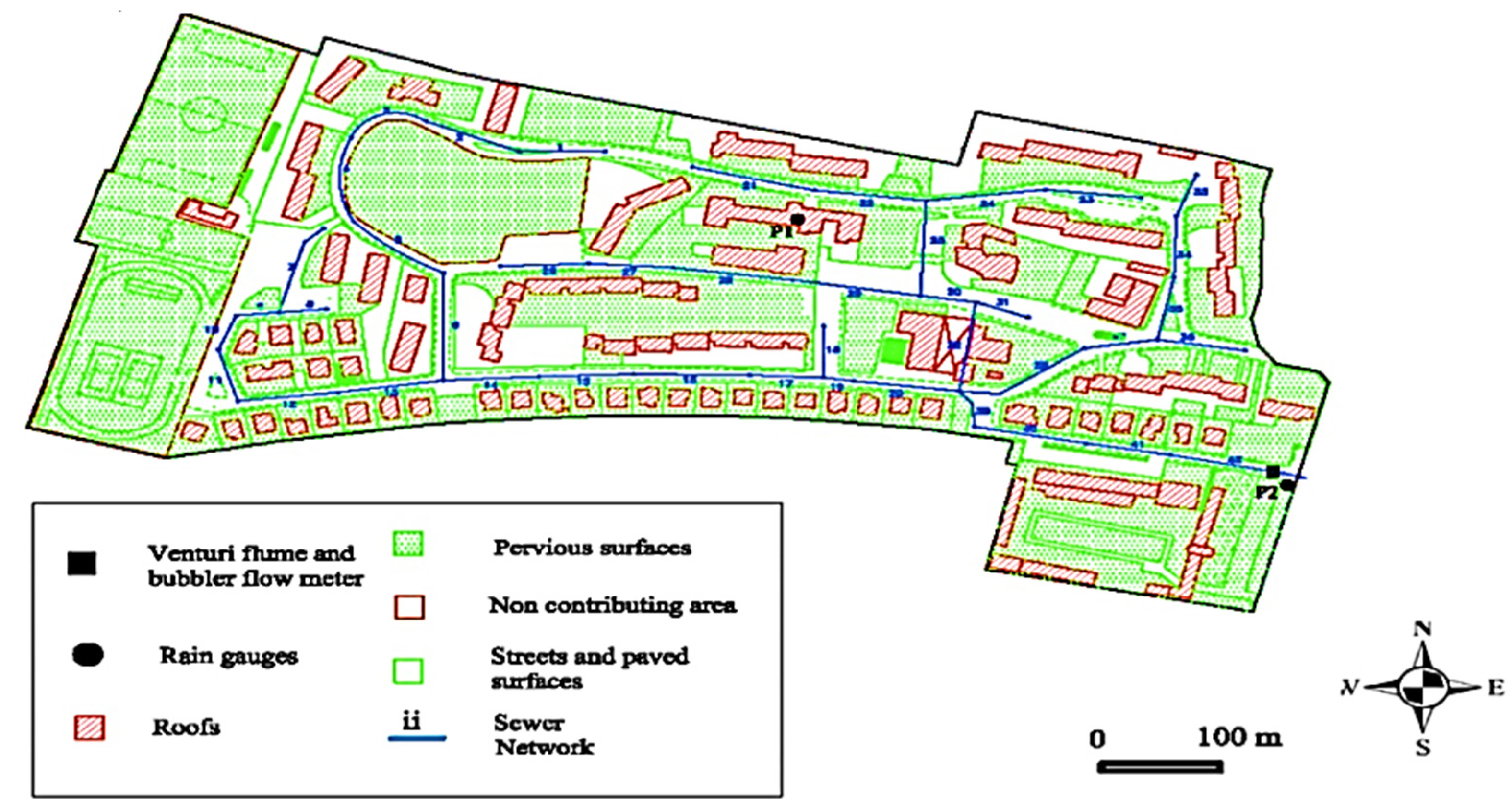
2. Case Study
- Regular operation of rain gages and flow meter without any instrumentation failures or pressurized flow conditions;
- Total rainfall depth of at least 5 mm;
- Maximum rainfall intensity equal to or greater than 0.1 mm/min;
- Maximum rainfall depth of at least 2 mm over 15 min.
3. Materials and Methods
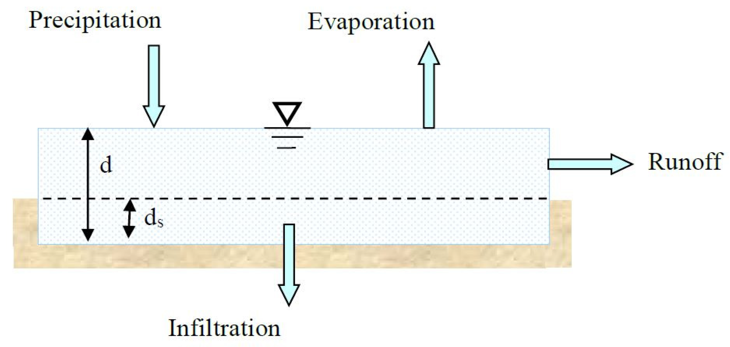
3.1. Non-Linear Reservoir (N-LR)
- Slope (-);
- Area (m2);
- Percentage of impervious and pervious area (-);
- Manning roughness coefficient for impervious area (roof) (s/m1/3);
- Manning roughness coefficient for impervious area (street) (s/m1/3);
- Manning roughness coefficient for the pervious area (s/m1/3);
- Depth of depression storage on impervious area (mm);
- Depth of depression storage on pervious area (mm);
- Maximum infiltration rate (mm/h);
- Minimum infiltration rate (mm/h);
- Decay coefficient (1/h);
- Maximum infiltration volume (mm);
- Drying time (days);
- Width coefficient (-).
- 15.
- Manning roughness for conduit (s/m1/3);
- 16.
- Conduit length (m);
- 17.
- Junction elevations (m);
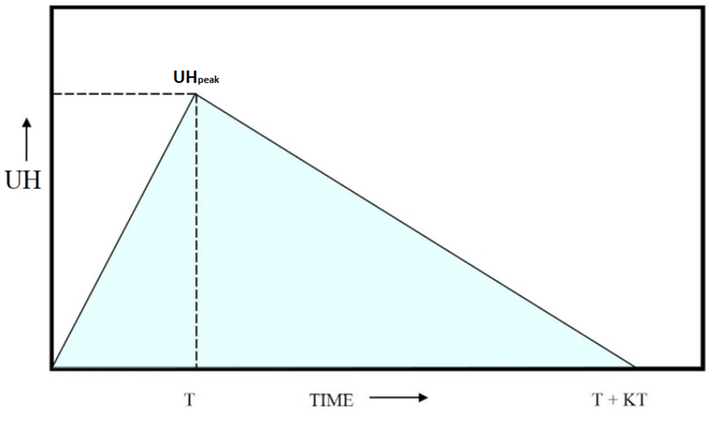
3.2. Unit Hydrograph (UH)
- R is the fraction of rainfall entering the channel network, also known as runoff volumetric coefficient (-);
- T is the time to peak (h);
- K is the ratio of time to recession to time to peak (-).
- Area (m2);
- Parameter R (-);
- Parameter T (h;
- Parameter K (-);
- 5.
- Manning roughness for the conduit (s/m1/3);
- 6.
- Conduit length (m);
- 7.
- Junction elevations (m).
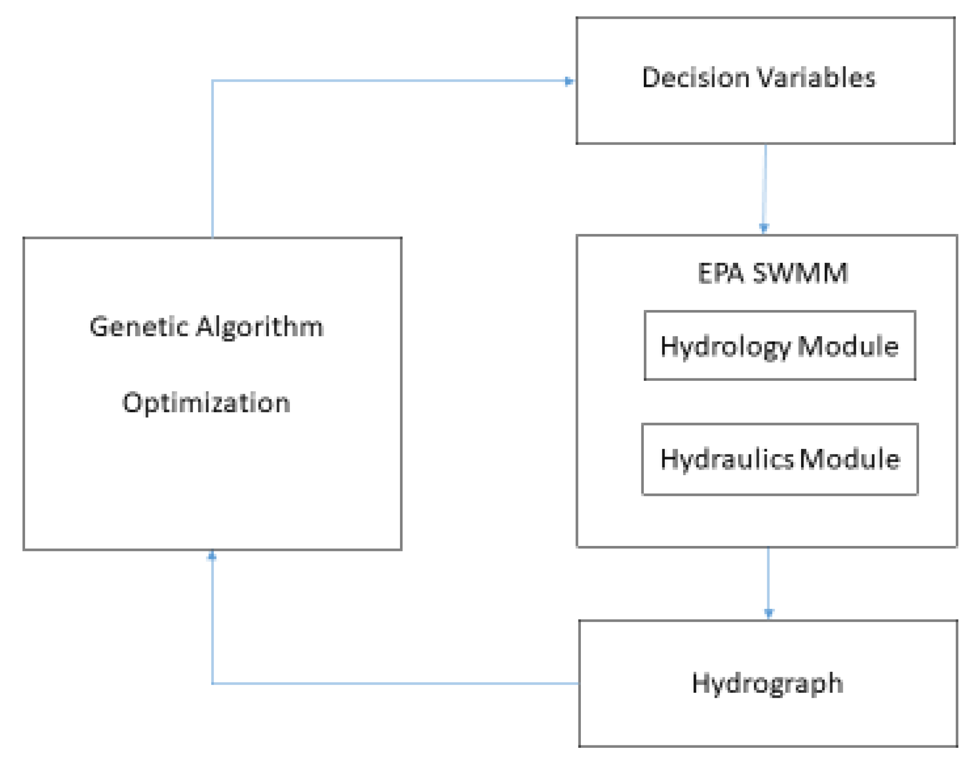
3.3. Genetic Optimization
3.4. Goodness-of-Fit Indices
4. Results
- -
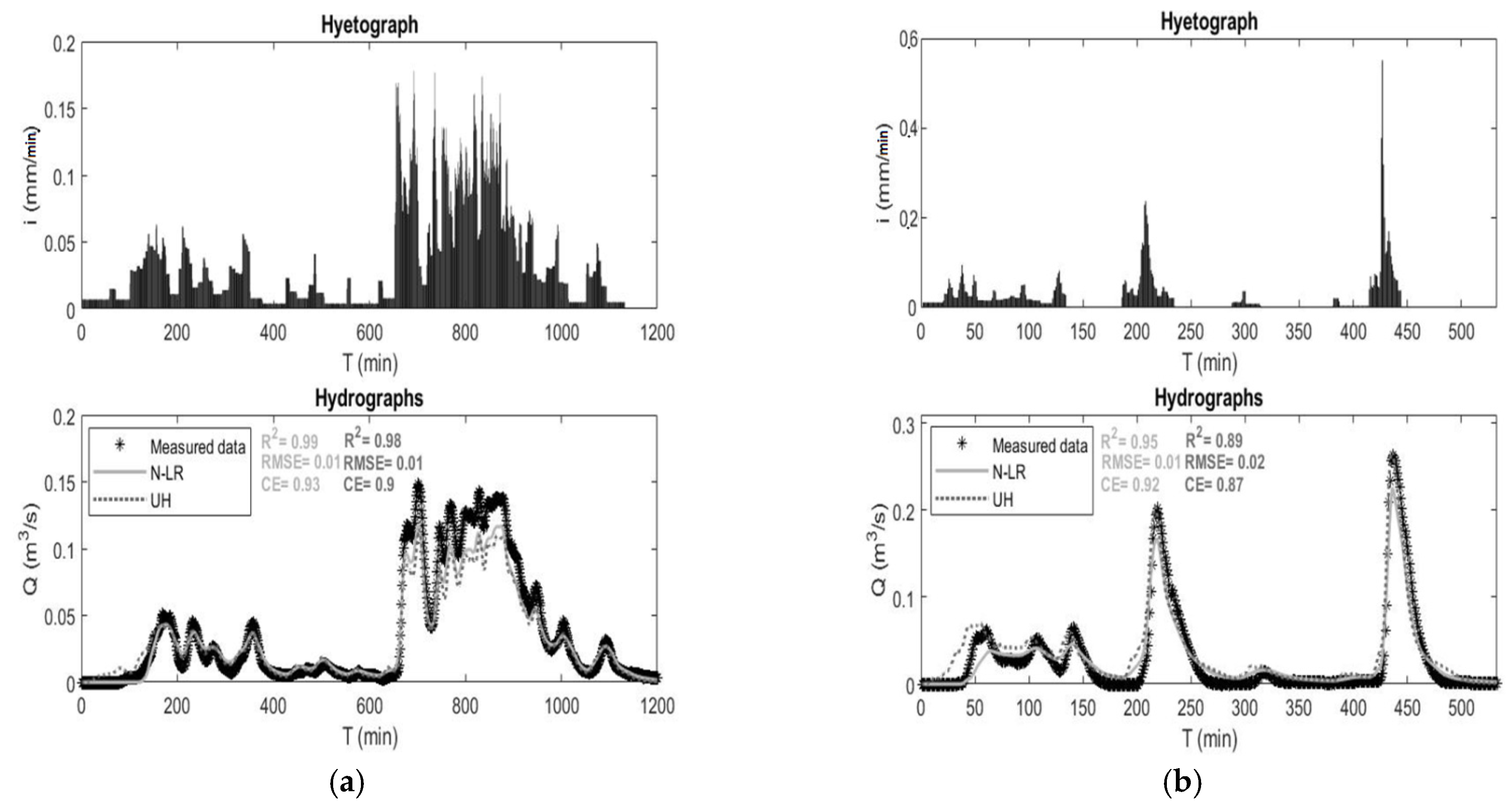
- In calibration, the N-LR method yields R2 = 0.99, RMSE = 0.01 m3/s, and CE = 0.93, whereas the UH method yields R2 = 0.98, RMSE = 0.01 m3/s, and CE = 0.90;
- -
- In validation, the N-LR method yields R2 = 0.95, RMSE = 0.01 m3/s, and CE = 0.92, whereas the UH method yields R2 = 0.89, RMSE = 0.02 m3/s, and CE = 0.87.
- -
- In calibration, looking at all the indices, the N-LR has a better performance in three events (7, 9, and 23); the UH prevails in two events (3 and 5); finally, the performance is similar in the remaining two events (14 and 17).
- -
- In validation, looking at all the indices, the N-LR is better in four events (8, 11, 12, and 13); the UH prevails in two events (20 and 21); finally, the performance is similar in the remaining event (19).
- -
- Globally, the N-RL seems to perform slightly better, also exhibiting higher performance in validation.
5. Discussion
Author Contributions
Funding
Institutional Review Board Statement
Informed Consent Statement
Data Availability Statement
Acknowledgments
Conflicts of Interest
References
- Zhu, Z.; Morales, V.; Garcia, M.H. Impact of combined sewer overflow on urban river hydrodynamic modelling: A case study of the Chicago waterway. Urban Water J. 2017, 14, 984–989. [Google Scholar] [CrossRef]
- Quijano, J.C.; Zhu, Z.; Morales, V.; Landry, B.J.; Garcia, M.H. Three-dimensional model to capture the fate and transport of combined sewer overflow discharges: A case study in the Chicago Area Waterway System. Sci. Total. Environ. 2017, 576, 362–373. [Google Scholar] [CrossRef] [PubMed]
- Todeschini, S. Hydrologic and environmental impacts of imperviousness in an industrial catchment of northern Italy. J. Hydrol. Eng. 2016, 21, 05016013. [Google Scholar] [CrossRef]
- Kourtis, I.M.; Tsihrintzis, V.A. Adaptation of urban drainage networks to climate change: A review. Sci. Total. Environ. 2021, 771, 145431. [Google Scholar] [CrossRef]
- Todeschini, S. Trends in long daily rainfall series of Lombardia (northern Italy) affecting urban storm water control. Int. J. Climatol. 2012, 32, 900–919. [Google Scholar] [CrossRef]
- Caviedes-Voullième, D.; Ahmadinia, E.; Hinz, C. Interactions of Microtopography, Slope and Infiltration Cause Complex Rainfall-Runoff Behavior at the Hillslope Scale for Single Rainfall Events. Water Resour. Res. 2021, 57, e2020WR028127. [Google Scholar] [CrossRef]
- Mohammadi, B. A review on the applications of machine learning for runoff modeling. Sustain. Water Resour. Manag. 2021, 7, 1–11. [Google Scholar] [CrossRef]
- Brocca, L.; Melone, F.; Moramarco, T. Distributed rainfall-runoff modelling for flood frequency estimation and flood fore-casting. Hydrol. Process. 2011, 25, 2801–2813. [Google Scholar] [CrossRef]
- Daniel, E.B.; Camp, J.V.; LeBoeuf, E.J.; Penrod, J.R.; Dobbins, J.P.; Abkowitz, M.D. Watershed modeling and its applications: A state-of-the-art review. Open Hydrol. J. 2011, 5, 27. [Google Scholar] [CrossRef] [Green Version]
- Peel, M.C.; McMahon, T.A. Historical development of rainfall-runoff modeling. WIREs Water 2020, 7, 1471. [Google Scholar] [CrossRef]
- Shin, M.J.; Guillaume, J.H.; Croke, B.F.; Jakeman, A.J. A review of foundational methods for checking the structural identi-fiability of models: Results for rainfall-runoff. J. Hydrol. 2015, 520, 1–16. [Google Scholar] [CrossRef]
- Javadinejad, S.; Dara, R.; Jafary, F. Difference of rainfall-runoff models and effect on flood forecasting: A brief review. Resour. Environ. Inf. Eng. 2022, 4, 184–199. [Google Scholar] [CrossRef]
- Kaffas, K.; Hrissanthou, V. Application of a continuous rainfall-runoff model to the basin of Kosynthos river using the hydrologic software HEC-HMS. Glob. NEST J. 2014, 16, 188–203. [Google Scholar]
- Yang, J.; Castelli, F.; Chen, Y. Multiobjective sensitivity analysis and optimization of distributed hydrologic model MOBIDIC. Hydrol. Earth Syst. Sci. 2014, 18, 4101–4112. [Google Scholar] [CrossRef] [Green Version]
- Khazaei, M.R.; Zahabiyoun, B.; Saghafian, B.; Ahmadi, S. Development of an Automatic Calibration Tool Using Genetic Algorithm for the ARNO Conceptual Rainfall-Runoff Model. Arab. J. Sci. Eng. 2013, 39, 2535–2549. [Google Scholar] [CrossRef]
- Paquet, E.; Garavaglia, F.; Garçon, R.; Gailhard, J. The SCHADEX method: A semi-continuous rainfall–runoff simulation for extreme flood estimation. J. Hydrol. 2013, 495, 23–37. [Google Scholar] [CrossRef]
- Gamage, S.; Hewa, G.; Beecham, S. Modelling hydrological losses for varying rainfall and moisture conditions in South Australian catchments. J. Hydrol. Reg. Stud. 2015, 4, 1–21. [Google Scholar] [CrossRef] [Green Version]
- Pinheiro, V.B.; Naghettini, M. Calibration of the Parameters of a Rainfall-Runoff Model in Ungauged Basins Using Synthetic Flow Duration Curves as Estimated by Regional Analysis. J. Hydrol. Eng. 2013, 18, 1617–1626. [Google Scholar] [CrossRef]
- Tan, S.B.; Chua, L.H.; Shuy, E.B.; Lo, E.Y.-M.; Lim, L.W. Performances of Rainfall-Runoff Models Calibrated over Single and Continuous Storm Flow Events. J. Hydrol. Eng. 2008, 13, 597–607. [Google Scholar] [CrossRef]
- Hossain, S.; Hewa, G.A.; Wella-Hewage, S. A Comparison of Continuous and Event-Based Rainfall–Runoff (RR) Modelling Using EPA-SWMM. Water 2019, 11, 611. [Google Scholar] [CrossRef] [Green Version]
- Nash, J.E. The form of the instantaneous unit hydrograph. Comptes Rendus Et Rapp. Assem. Gen. De Tor. 1957, 3, 114–121. [Google Scholar]
- Chen, C.W.; Shubinski, R.P. Computer Simulation of Urban Storm Water Runoff. J. Hydraul. Div. 1971, 97, 289–301. [Google Scholar] [CrossRef]
- Rossman, L.A. Storm Water Management Model User’s Manual, Version 5.0; National Risk Management Research Laboratory, Office of Research and Development, US Environmental Protection Agency: Cincinnati, OH, USA, 2010.
- Niazi, M.; Nietch, C.; Maghrebi, M.; Jackson, N.; Bennett, B.R.; Tryby, M.; Massoudieh, A. Storm Water Management Model: Performance Review and Gap Analysis. J. Sustain. Water Built Environ. 2017, 3, 04017002. [Google Scholar] [CrossRef] [Green Version]
- Rossman, L.; Huber, W. Storm Water Management Model Reference Manual; EPA/600/R-15/162A; U.S. EPA Office of Research and Development: Washington, DC, USA, 2015; Volume 1.
- Wang, W.-C.; Cheng, C.-T.; Chau, K.-W.; Xu, D.-M. Calibration of Xinanjiang model parameters using hybrid genetic algorithm based fuzzy optimal model. J. Hydroinform. 2011, 14, 784–799. [Google Scholar] [CrossRef] [Green Version]
- Sarkar, A.; Kumar, R. Artificial Neural Networks for Event Based Rainfall-Runoff Modeling. J. Water Resour. Prot. 2012, 04, 891–897. [Google Scholar] [CrossRef] [Green Version]
- Shamsi, U.M.S.; Koran, J. Continuous calibration. J. Water Manag. Model. 2017, 25, C414. [Google Scholar] [CrossRef] [Green Version]
- Alamdari, N. Development of a robust automated tool for calibrating a SWMM watershed model. World Environ. Water Resour. Congr. 2016, 221–228. [Google Scholar] [CrossRef]
- Behrouz, M.S.; Zhu, Z.; Matott, L.S.; Rabideau, A.J. A new tool for automatic calibration of the Storm Water Management Model (SWMM). J. Hydrol. 2019, 581, 124436. [Google Scholar] [CrossRef]
- Barco, J.; Wong, K.M.; Stenstrom, M.K. Automatic Calibration of the U.S. EPA SWMM Model for a Large Urban Catchment. J. Hydraul. Eng. 2008, 134, 466–474. [Google Scholar] [CrossRef]
- Chow, M.F.; Yusop, Z.; Toriman, M.E. Modelling runoff quantity and quality in tropical urban catchments using Storm Water Management Model. Int. J. Environ. Sci. Technol. 2012, 9, 737–748. [Google Scholar] [CrossRef] [Green Version]
- Xing, W.; Li, P.; Cao, S.-B.; Gan, L.-L.; Liu, F.-L.; Zuo, J.-E. Layout effects and optimization of runoff storage and filtration facilities based on SWMM simulation in a demonstration area. Water Sci. Eng. 2016, 9, 115–124. [Google Scholar] [CrossRef] [Green Version]
- Masseroni, D.; Cislaghi, A. Green roof benefits for reducing flood risk at the catchment scale. Environ. Earth Sci. 2016, 75, 1–11. [Google Scholar] [CrossRef]
- Holland, J.H. Genetic Algorithms and the Optimal Allocation of Trials. SIAM J. Comput. 1973, 2, 88–105. [Google Scholar] [CrossRef]
- Huang, J.J.; Xiao, M.; Li, Y.; Yan, R.; Zhang, Q.; Sun, Y.; Zhao, T. The optimization of Low Impact Development placement considering life cycle cost using Genetic Algorithm. J. Environ. Manag. 2022, 309, 114700. [Google Scholar] [CrossRef] [PubMed]
- Tetzlaff, D.; Soulsby, C.; Waldron, S.; Malcolm, I.A.; Bacon, P.J.; Dunn, S.M.; Lilly, A.; Youngson, A.F. Conceptualization of runoff processes using a geographical information system and tracers in a nested mesoscale catchment. Hydrol. Process. 2006, 21, 1289–1307. [Google Scholar] [CrossRef]
- Gupta, A.K.; Shrivastava, R.K. Optimal design of water treatment plant under uncertainty using genetic algorithm. Environ. Prog. 2008, 27, 91–97. [Google Scholar] [CrossRef]
- Chlumecký, M.; Buchtele, J.; Richta, K. Application of random number generators in genetic algorithms to improve rain-fall-runoff modelling. J. Hydrol. 2017, 553, 350–355. [Google Scholar] [CrossRef]
- Lopes, M.D.; da Silva, G.B.L. An efficient simulation-optimization approach based on genetic algorithms and hydrologic modeling to assist in identifying optimal low impact development designs. Landsc. Urban Plan. 2021, 216, 104251. [Google Scholar] [CrossRef]
- Papiri, S.; Ciaponi, C.; Todeschini, S. Il bacino urbano sperimentale di Cascina Scala (Pavia). Aracne Via Raffaele Garofalo. 2008, 217, 133. [Google Scholar]
- Barco, J.; Papiri, S.; Stenstrom, M.K. First flush in a combined sewer system. Chemosphere 2008, 71, 827–833. [Google Scholar] [CrossRef] [PubMed]
- Giguere, P.R.; Riek, G.C. Infiltration/Inflow Modeling for the East Bay (Oakland-Berkeley Area) I/I Study. In Proceedings of the 1983 International Symposium on Urban Hydrology, Hydraulics and Sediment Control, Lexington, KY, USA, 25–28 July 1983. [Google Scholar]
- Vallabhaneni, S.; Chan, C.; Burgess, E.H. Computer Tools for Sanitary Sewer System Capacity Analysis and Planning; US Environmental Protection Agency, Office of Research Development: Washington, DC, USA, 2007.
- Moriasi, D.N.; Arnold, J.G.; Van Liew, M.W.; Bingner, R.L.; Harmel, R.D.; Veith, T.L. Model evaluation guidelines for sys-tematic quantification of accuracy in watershed simulations. Trans. ASABE 2007, 50, 885–900. [Google Scholar] [CrossRef]
- Krebs, G.; Kokkonen, T.; Valtanen, M.; Koivusalo, H.; Setälä, H. A high resolution application of a stormwater management model (SWMM) using genetic parameter optimization. Urban Water J. 2013, 10, 394–410. [Google Scholar] [CrossRef]
- Zakizadeh, F.; Nia, A.M.; Salajegheh, A.; Sañudo-Fontaneda, L.A.; Alamdari, N. Efficient Urban Runoff Quantity and Quality Modelling Using SWMM Model and Field Data in an Urban Watershed of Tehran Metropolis. Sustainability 2022, 14, 1086. [Google Scholar] [CrossRef]
- Fowler, K.; Peel, M.; Western, A.; Zhang, L. Improved rainfall-runoff calibration for drying climate: Choice of objective function. Water Resour. Res. 2018, 54, 3392–3408. [Google Scholar] [CrossRef]


| ID | A (ha) | S (%) | IA | ID | A (ha) | S (%) | IA | ||
|---|---|---|---|---|---|---|---|---|---|
| R (%) | S&S (%) | R (%) | S&S (%) | ||||||
| 1 | 0.27 | 0.5 | 0 | 29.2 | 22 | 0.50 | 0.5 | 20.4 | 56.3 |
| 2 | 0.20 | 0.2 | 21.2 | 54.8 | 23 | 0.13 | 0.1 | 0 | 85.9 |
| 3 | 0.39 | 0.1 | 23.1 | 40.7 | 24 | 0.81 | 0.1 | 23.5 | 47.8 |
| 4 | 0.28 | 0.1 | 32.8 | 54.4 | 25 | 0.41 | 0.2 | 24.2 | 31.9 |
| 5 | 0.07 | 0.1 | 0 | 100 | 26 | 0.13 | 0.1 | 0 | 100 |
| 6 | 0.49 | 0.1 | 32.5 | 40 | 27 | 0.39 | 0.1 | 22.1 | 26 |
| 7 | 0.09 | 0.1 | 0 | 100 | 28 | 0.21 | 0.1 | 37.9 | 9 |
| 8 | 0.16 | 0.1 | 32.4 | 33.2 | 29 | 0.20 | 0.1 | 0 | 77.9 |
| 9 | 0.07 | 0.1 | 24.5 | 43.2 | 30 | 0.06 | 0.1 | 0 | 75.4 |
| 10 | 0.57 | 0.1 | 5.1 | 35.6 | 31 | 0.10 | 0.1 | 0 | 80.8 |
| 11 | 0.12 | 0.1 | 12.4 | 62.7 | 32 | 0.50 | 0.1 | 37.6 | 21.9 |
| 12 | 0.36 | 0.3 | 30.8 | 30.5 | 33 | 0.05 | 0.2 | 19.5 | 80.5 |
| 13 | 0.20 | 0.3 | 31.3 | 46.8 | 34 | 0.33 | 0.1 | 23.1 | 40.2 |
| 14 | 0.16 | 0.1 | 20.3 | 53 | 35 | 0.42 | 0.1 | 32 | 41.5 |
| 15 | 1.35 | 0.1 | 26.3 | 25.6 | 36 | 0.27 | 0.1 | 16 | 40.7 |
| 16 | 0.21 | 0.1 | 29.3 | 37.1 | 37 | 0.24 | 0.1 | 16.3 | 65.7 |
| 17 | 0.11 | 0.1 | 23.9 | 43.4 | 38 | 0.16 | 0.2 | 14.4 | 51.9 |
| 18 | 0.06 | 0.3 | 0 | 100 | 39 | 0.05 | 0.1 | 0 | 48 |
| 19 | 0.05 | 0.1 | 30.6 | 54.3 | 40 | 0.19 | 0.6 | 29.6 | 43.9 |
| 20 | 0.17 | 0.1 | 26.2 | 42 | 41 | 0.12 | 0.3 | 25.2 | 49.6 |
| 21 | 0.47 | 0.1 | 26.5 | 29.3 | 42 | 0.22 | 0.3 | 26.8 | 57.3 |
| 42 * | 1.55 | 0.3 | 25.1 | 21.1 | |||||
| Event | Total Rainfall Depth Vtotal (mm) | Rainfall Duration Ttotal (min) | Peak Flow Rate QMax (m3/s) |
|---|---|---|---|
| 3 | 11.8 | 197 | 0.255 |
| 5 | 16.4 | 108 | 0.551 |
| 7 | 7 | 50 | 0.326 |
| 9 | 10.6 | 215 | 0.19 |
| 14 | 15.8 | 380 | 0.257 |
| 17 | 23.4 | 964 | 0.139 |
| 23 | 39.8 | 1133 | 0.149 |
| 8 | 11 | 64 | 0.376 |
| 11 | 26.2 | 478 | 0.281 |
| 12 | 18.6 | 443 | 0.263 |
| 13 | 8.4 | 111 | 0.157 |
| 19 | 12.6 | 248 | 0.234 |
| 20 | 16.2 | 231 | 0.245 |
| 21 | 7 | 286 | 0.06 |
| Parameter | Range of Variation | Calibrated Value |
|---|---|---|
| Manning coefficient for roof (s/m1/3) | 0.014–0.030 | 0.014 |
| Manning coefficient for street (s/m1/3) | 0.010–0.055 | 0.011 |
| Manning coefficient for pervious area (s/m1/3) | 0.10–0.35 | 0.321 |
| Depression storage on impervious area (mm) | 1.27–2.54 | 1.27 |
| Depression storage on pervious area (mm) | 2.54–5.08 | 3.08 |
| Maximum infiltration rate (mm/h) | 58–170 | 118 |
| Minimum infiltration rate (mm/h) | 1–57 | 50 |
| Decay coefficient (1/h) | 2–7 | 4.3 |
| Width coefficient (-) | 1–2 | 1.99 |
| Manning coefficient for conduit (s/m1/3) | 0.012–0.02 | 0.012 |
| N | R (-) | T (h) | K (-) | |||
|---|---|---|---|---|---|---|
| Range of Variation | Calibrated Value | Range of Variation | Calibrated Value | Range of Variation | Calibrated Value | |
| 1 | 0.23–0.35 | 0.24 | 0.08–0.33 | 0.33 | 0.5–2 | 1.99 |
| 2 | 0.61–0.91 | 0.63 | 0.08–0.33 | 0.32 | 0.5–2 | 1.46 |
| 3 | 0.51–0.77 | 0.51 | 0.08–0.33 | 0.08 | 0.5–2 | 0.57 |
| 4 | 0.7–1 | 0.73 | 0.08–0.33 | 0.09 | 0.5–2 | 0.53 |
| 5 | 0.8–1 | 0.8 | 0.08–0.33 | 0.33 | 0.5–2 | 2 |
| 6 | 0.58–0.87 | 0.58 | 0.08–0.33 | 0.33 | 0.5–2 | 1.88 |
| 7 | 0.8–1 | 0.8 | 0.08–0.33 | 0.17 | 0.5–2 | 0.62 |
| 8 | 0.52–0.79 | 0.53 | 0.08–0.33 | 0.1 | 0.5–2 | 0.69 |
| 9 | 0.54–0.81 | 0.61 | 0.08–0.33 | 0.09 | 0.5–2 | 0.52 |
| 10 | 0.33–0.49 | 0.37 | 0.08–0.33 | 0.33 | 0.5–2 | 2 |
| 11 | 0.6–0.9 | 0.67 | 0.08–0.33 | 0.08 | 0.5–2 | 0.57 |
| 12 | 0.49–0.74 | 0.55 | 0.08–0.33 | 0.08 | 0.5–2 | 0.56 |
| 13 | 0.62–0.94 | 0.64 | 0.08–0.33 | 0.33 | 0.5–2 | 1.97 |
| 14 | 0.59–0.88 | 0.59 | 0.08–0.33 | 0.08 | 0.5–2 | 0.56 |
| 15 | 0.42–0.62 | 0.53 | 0.08–0.33 | 0.09 | 0.5–2 | 0.55 |
| 16 | 0.53–0.8 | 0.69 | 0.08–0.33 | 0.08 | 0.5–2 | 0.52 |
| 17 | 0.54–0.81 | 0.57 | 0.08–0.33 | 0.09 | 0.5–2 | 0.56 |
| 18 | 0.8–1 | 0.91 | 0.08–0.33 | 0.08 | 0.5–2 | 1.5 |
| 19 | 0.68–1 | 1 | 0.08–0.33 | 0.08 | 0.5–2 | 0.5 |
| 20 | 0.55–0.82 | 0.82 | 0.08–0.33 | 0.09 | 0.5–2 | 0.5 |
| 21 | 0.45–0.67 | 0.48 | 0.08–0.33 | 0.27 | 0.5–2 | 1.91 |
| 22 | 0.61–0.92 | 0.62 | 0.08–0.33 | 0.33 | 0.5–2 | 1.68 |
| 23 | 0.69–1 | 0.72 | 0.08–0.33 | 0.09 | 0.5–2 | 1.37 |
| 24 | 0.57–0.86 | 0.62 | 0.08–0.33 | 0.08 | 0.5–2 | 0.5 |
| 25 | 0.45–0.67 | 0.58 | 0.08–0.33 | 0.08 | 0.5–2 | 0.5 |
| 26 | 0.8–1 | 0.94 | 0.08–0.33 | 0.08 | 0.5–2 | 0.5 |
| 27 | 0.38–0.58 | 0.58 | 0.08–0.33 | 0.3 | 0.5–2 | 1.2 |
| 28 | 0.38–0.56 | 0.44 | 0.08–0.33 | 0.08 | 0.5–2 | 0.89 |
| 29 | 0.62–0.93 | 0.63 | 0.08–0.33 | 0.33 | 0.5–2 | 1.86 |
| 30 | 0.6–0.9 | 0.72 | 0.08–0.33 | 0.1 | 0.5–2 | 0.52 |
| 31 | 0.65–0.97 | 0.7 | 0.08–0.33 | 0.33 | 0.5–2 | 1.7 |
| 32 | 0.48–0.71 | 0.48 | 0.08–0.33 | 0.08 | 0.5–2 | 1.16 |
| 33 | 0.8–1 | 0.97 | 0.08–0.33 | 0.08 | 0.5–2 | 0.52 |
| 34 | 0.51–0.76 | 0.7 | 0.08–0.33 | 0.08 | 0.5–2 | 0.51 |
| 35 | 0.59–0.88 | 0.59 | 0.08–0.33 | 0.1 | 0.5–2 | 0.79 |
| 36 | 0.45–0.68 | 0.67 | 0.08–0.33 | 0.08 | 0.5–2 | 0.58 |
| 37 | 0.66–0.98 | 0.98 | 0.08–0.33 | 0.08 | 0.5–2 | 0.59 |
| 38 | 0.53–0.8 | 0.59 | 0.08–0.33 | 0.08 | 0.5–2 | 0.59 |
| 39 | 0.38–0.58 | 0.4 | 0.08–0.33 | 0.16 | 0.5–2 | 0.5 |
| 40 | 0.59–0.88 | 0.88 | 0.08–0.33 | 0.09 | 0.5–2 | 0.6 |
| 41 | 0.6–0.9 | 0.9 | 0.08–0.33 | 0.08 | 0.5–2 | 0.83 |
| 42 | 0.37–0.55 | 0.55 | 0.08–0.33 | 0.21 | 0.5–2 | 1.5 |
| 42 * | 0.67–1 | 0.99 | 0.08–0.33 | 0.09 | 0.5–2 | 0.6 |
| Event | R2 (-) | RSME (m3/s) | CE (-) | ||||
|---|---|---|---|---|---|---|---|
| N-LR | UH | N-LR | UH | N-LR | UH | ||
| Calibration | 3 | 0.78 | 0.87 | 0.03 | 0.02 | 0.77 | 0.85 |
| 5 | 0.92 | 0.96 | 0.03 | 0.03 | 0.91 | 0.94 | |
| 7 | 0.51 | 0.42 | 0.07 | 0.08 | 0.50 | 0.30 | |
| 9 | 0.90 | 0.86 | 0.02 | 0.02 | 0.69 | 0.58 | |
| 14 | 0.94 | 0.94 | 0.02 | 0.02 | 0.88 | 0.86 | |
| 17 | 0.91 | 0.91 | 0.01 | 0.01 | 0.72 | 0.74 | |
| 23 | 0.99 | 0.98 | 0.01 | 0.01 | 0.93 | 0.90 | |
| Validation | 8 | 0.81 | 0.68 | 0.04 | 0.06 | 0.81 | 0.57 |
| 11 | 0.98 | 0.96 | 0.01 | 0.01 | 0.95 | 0.95 | |
| 12 | 0.95 | 0.89 | 0.01 | 0.02 | 0.92 | 0.87 | |
| 13 | 0.94 | 0.82 | 0.02 | 0.02 | 0.85 | 0.78 | |
| 19 | 0.97 | 0.97 | 0.02 | 0.02 | 0.91 | 0.92 | |
| 20 | 0.69 | 0.75 | 0.03 | 0.03 | 0.51 | 0.58 | |
| 21 | 0.85 | 0.88 | 0.01 | 0.01 | 0.49 | 0.44 | |
Disclaimer/Publisher’s Note: The statements, opinions and data contained in all publications are solely those of the individual author(s) and contributor(s) and not of MDPI and/or the editor(s). MDPI and/or the editor(s) disclaim responsibility for any injury to people or property resulting from any ideas, methods, instructions or products referred to in the content. |
© 2023 by the authors. Licensee MDPI, Basel, Switzerland. This article is an open access article distributed under the terms and conditions of the Creative Commons Attribution (CC BY) license (https://creativecommons.org/licenses/by/4.0/).
Share and Cite
Giudicianni, C.; Assaf, M.N.; Todeschini, S.; Creaco, E. Comparison of Nonlinear Reservoir and UH Algorithms for the Hydrological Modeling of a Real Urban Catchment with EPASWMM. Hydrology 2023, 10, 24. https://0-doi-org.brum.beds.ac.uk/10.3390/hydrology10010024
Giudicianni C, Assaf MN, Todeschini S, Creaco E. Comparison of Nonlinear Reservoir and UH Algorithms for the Hydrological Modeling of a Real Urban Catchment with EPASWMM. Hydrology. 2023; 10(1):24. https://0-doi-org.brum.beds.ac.uk/10.3390/hydrology10010024
Chicago/Turabian StyleGiudicianni, Carlo, Mohammed N. Assaf, Sara Todeschini, and Enrico Creaco. 2023. "Comparison of Nonlinear Reservoir and UH Algorithms for the Hydrological Modeling of a Real Urban Catchment with EPASWMM" Hydrology 10, no. 1: 24. https://0-doi-org.brum.beds.ac.uk/10.3390/hydrology10010024