Assessment of Time Series Models for Mean Discharge Modeling and Forecasting in a Sub-Basin of the Paranaíba River, Brazil

Abstract

Stochastic modeling to forecast hydrological variables under changing climatic conditions is essential for water resource management and adaptation planning. This study explores the applicability of stochastic models, specifically SARIMA and SARIMAX, to forecast monthly average river discharge in a sub-basin of the Paranaíba River near Patos de Minas, MG, Brazil. The Paranaíba River is a vital water source for the Alto Paranaíba region, serving industrial supply, drinking water effluent dilution for urban communities, agriculture, fishing, and tourism. The study evaluates the performance of SARIMA and SARIMAX models in long-term discharge modeling and forecasting, demonstrating the SARIMAX model’s superior performance in various metrics, including the Nash–Sutcliffe coefficient (NSE), the root mean square error (RMSE), and the mean absolute percentage error (MAPE). The inclusion of precipitation as a regressor variable considerably improves the forecasting accuracy, and can be attributed to the multivariate structure of the SARIMAX model. While stochastic models like SARIMAX offer valuable decision-making tools for water resource management, the study underscores the significance of employing long-term time series encompassing flood and drought periods and including model uncertainty analysis to enhance the robustness of forecasts. In this study, the SARIMAX model provides a better fit for extreme values, overestimating peaks by around 11.6% and troughs by about 5.0%, compared with the SARIMA model, which tends to underestimate peaks by an average of 6.5% and overestimate troughs by approximately 76.0%. The findings contribute to the literature on water management strategies and mitigating risks associated with extreme hydrological events.

1. Introduction

Efficient management of available water resources requires adequate hydrological forecasting models. This need arises due to the increasing water demand linked to population growth and economic development [1,2]. Hydrological time series modeling holds significant importance due to its various applications, including drought management, flood forecasting, discharge (streamflow) forecasting, and environmental management, among other uses [3,4,5,6]. Hydrological models are classified differently based on the type of variables they use and the relationship between them, the data representation method, the existence of spatial relationships, and temporal dependencies [7].

It is possible to categorize hydrological models into two main categories: those based on physical processes and the area’s physical characteristics and data-driven models mainly based on time series data analysis. Models based on physical processes have as their main limitation their complexity, which leads to high computational efforts and a large volume of required input data [8]. On the other hand, data-driven models, including time series models, deep learning, and machine learning models, require care in the calibration of their hyperparameters [9]. Hybrid approaches, combining physical and data-driven models, are gaining prominence in this field [10]. These approaches leverage the strengths of numerical hydrological models. By fusing the physics-based understanding of hydrological processes with the data-driven capacity to capture complex relationships, hybrid models offer robust streamflow forecasts, particularly in regions with limited data or rapidly changing hydrological conditions [9,11,12].

Hydrological forecasting is carried out following two modeling approaches: deterministic and stochastic [3,6]. Most hydrological processes are stochastic, meaning they involve mathematical models incorporating random elements. The prevalence of stochasticity in hydrology derives from the complex and unpredictable nature of hydrological phenomena. However, despite their inherent randomness, hydrological processes exhibit seasonal patterns, periodic regularities, and discernible deterministic factors. These processes can be analyzed using principles of mass, energy, momentum conservation, and thermodynamics, as well as conceptual and empirical models commonly employed in modern physical hydrology [13]. Over recent years, the combination of both approaches has been instrumental in developing and calibrating hydrological models, as this integrated approach has been proven to be helpful in developing an understanding of the intricate interplay between natural and anthropogenic processes within watersheds [14,15,16], thus enhancing the effectiveness of decision-making in water resource system analysis.

Hydrological time series are sequences of water-related data points collected over time. These data points encompass measurements of various variables (e.g., rainfall, river flow, and groundwater levels), and they are analyzed with the primary goal of methodically identifying and describing the underlying generating processes responsible for a specific sequence of observations [17]. Their modeling examines the dynamic system characterized by input and output sequences connected through a function. There are two main types of time series techniques: univariate and multivariate. Univariate methods explain the output series using elements such as constant components, trends, seasonality, or even lagged portions of the series under analysis. Multivariate methods, on the other hand, aim to improve the representation of the underlying transfer function by considering the influence of other variables on the behavior of the output series [18].

AutoRegressive integrated moving average (ARIMA) models, introduced by Box and Jenkins in the 1970s [19], are widely applied in time series analysis as linear statistical models for representing and capturing the features of time series data generated by stochastic processes [20]. Furthermore, the parameters of an ARIMA model can be fitted to convert it into autoregressive (AR), moving average (MA), or autoregressive moving average models (ARMA) models [17]. Of particular interest for this study are the SARIMA and SARIMAX models, extensions created to manage time series data with seasonal characteristics and primarily used for forecasting when there are evident seasonal patterns or variations in the data. The SARIMAX model is a multivariate version of the SARIMA model, allowing the integration of exogenous (explanatory) variables to increase its forecasting performance [21]. Incorporating additional climatological variables, such as temperature [22] and evapotranspiration [23], may enhance model performance and provide a deeper understanding of river discharge patterns. These additional variables could contribute to more robust and accurate hydrological models, particularly in the context of a changing climate and evolving land use patterns.

Brazil’s abundant water resources support biodiversity and the economy, and the country boasts the world’s largest share of renewable internal freshwater resources, comprising 12% of the globe’s total. Water is vital for agriculture and hydropower, but current challenges, such as uneven distribution and governance issues, must be overcome to guarantee sustainable development [24]. In 2021, the Brazilian National Water and Sanitation Agency (Agência Nacional de Águas e Saneamento Básico—ANA) published a water resources conjuncture report for the country. This report underscores the rising water demand, particularly in the industrial, agricultural, and human supply sectors. Projections indicate a 42% increase in water resource consumption by 2040, highlighting the urgent need for strategic planning and adequate forecasting to ensure safe water usage, mitigate the risk of water crises, and support various water-related needs, all while considering the impact of climate change on the hydrological cycle [25].

Water-related disasters (both droughts and floods) have acquired global attention due to their impacts on vulnerable communities and their increasing occurrence in the face of climate change [26,27], and this is also observed in Brazil [28,29,30]. According to Souza et al. [31], there are over 40,000 areas at risk of hydrological disasters in Brazil, which together encompass around 120 million people and are responsible for 60% of the gross domestic product. Despite national regulations, local efforts to build resilience to floods, landslides, droughts, biodiversity loss, and energy consumption are slow. The National Center for Monitoring and Natural Disaster Alert (CEMADEN) highlights that available hydrometeorological data for developing mitigation actions is usually scarce, thus emphasizing the need to develop methodologies for water resource management that are capable of overcoming data scarcity limitations [32]. In this scenario, stochastic analysis provides effective decision-making tools for managing water resources in regions with limited data. This allows for the inclusion of natural uncertainty and variations in hydrological processes, thereby improving the efficacy of water management strategies in uncertain conditions [14].

Many researchers have relied on ARIMA, SARIMA, and SARIMAX for streamflow modeling worldwide. Examples in the literature include the paper by Kassem et al. [33], who applied the ARIMA model for simulating daily flow at the Khazir River basin in Iraq, obtaining R² values of about 0.77 and 0.82 for the two monitoring stations in the catchment. Sun et al. [34] tested the performance of a combination of the ARIMA model with wavelet transform in the Heihe River basin of northern China and the Pearl River basin of southern China. They obtained R² values above 0.83 for all of the monitoring locations in the validation set. Danandeh Mehr et al. [35] showed satisfactory results when using the SARIMA model for streamflow forecasting on one-step-ahead daily and weekly scales at the Oulujoki River system in northeastern Finland. However, intramonthly streamflow forecasting exhibited low accuracy. Thus, they introduced an ensemble univariate genetic programming–SARIMA model and improved its accuracy significantly.

Furthermore, significant researchers in this sense were also developed in Brazilian catchments. For instance, Bayer et al. [36] used a SARIMA model to forecast monthly discharges in the Potiribu River basin, obtaining a Nash–Sutcliffe coefficient of 0.81 for six-month-ahead projections. Chechi and Sanches [37] employed maximum and minimum temperatures and the climatological normal of precipitation as covariates with which to configure a SARIMAX model for precipitation in Erechim. This model exhibited a high correlation between measurements and simulated values, except for extreme values that were possibly associated with the ENSO phenomenon. Pinto et al. [38] used SARIMA models and long-term records to forecast the monthly average flow in the Doce River watershed in Espirito Santo. In the same state, Bleidorn et al. [23] attempted to model and forecast monthly average flows in the Jucu River. However, they encountered challenges in accurately predicting flows due to a severe water crisis, the most significant in 80 years, which introduced significant biases despite satisfactory results obtained during the training period. Caixeta et al. [39] also experienced these adverse effects when employing SARIMA class models for forecasting mean monthly discharges in a Paranaíba River basin in the Alto Paranaíba region. The negative Nash–Sutcliffe coefficient between measurements and forecasts highlighted the limitations of stochastic models in water scarcity scenarios. In these two latter studies, the authors recommend the inclusion of other regressor variables, consequently applying a SARIMAX model to improve accuracy in the face of extreme event scenarios.

The present study aims to assess the suitability and effectiveness of ARIMA class models, specifically SARIMA and SARIMAX, for long-term monthly average discharge forecasting for a sub-basin of the Paranaíba River near Patos de Minas, MG. This case study configures an illustrative example in the context of urban water management and environmental challenges, as the Paranaiba River serves as both a water source and sewage receiver for the population of Patos de Minas, a region rapidly developing and with a considerable production for grain, livestock, and dairy [40]. Additionally, this paper discusses how stochastic modeling can aid in forecasting streamflow under changing climatic conditions, addressing the increasing demand for water resources, and contributing to its effective management.

2. Materials and Methods

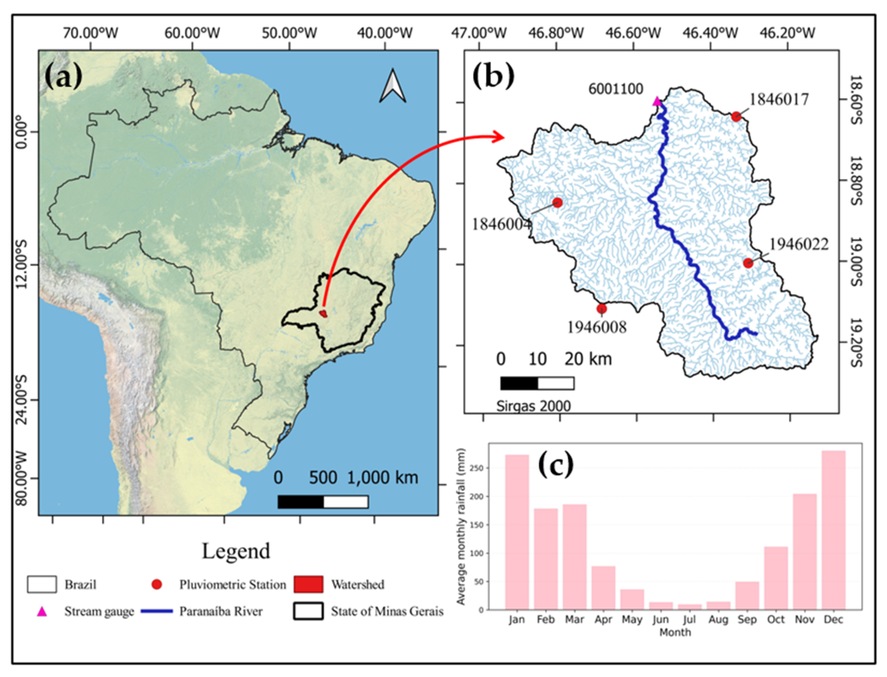
2.1. Study Area and Gauging Stations

The study employs hydrological data from a sub-basin of the Paranaíba River, a major tributary within the Paraná River basin. The outlet for this sub-basin is at the fluviometric station named Patos de Minas, as depicted in Figure 1. This station is situated at geographical coordinates of longitude 46°32′21.84″ west and latitude 18°36′6.12″ south, located within Patos de Minas, MG [41].

Patos de Minas is located within the Mesoregion of Triângulo Mineiro and Alto Paranaíba. It covers an area of 3190.5 km², encompassing a population of approximately 159,000 people [42]. Figure 1c shows that rainfall in this region occurs from October to April, with a dry period from May to September, and average temperatures ranging from 18–22 °C in June to 22–26 °C in December. The municipality of Patos de Minas is situated in an area characterized by the Central Brazil Tropical Climate, featuring four to five dry months. This climatological regime falls under the sub-classification of the Central Brazil Wet–Dry or Central Brazil Tropical Climate [43], which aligns with the Aw type classification in the Köppen–Geiger climate system, signifying a tropical climate [44].

Patos de Minas holds a prominent position in the region due to its role as an agricultural hub, especially for grains, livestock, and dairy production [45]. It is also an economic center supporting various businesses and industries, an educational and healthcare hub offering services to the region, and a transportation hub with well-connected road networks, making Patos de Minas one of the cities with the best ratings in terms of quality of life in the state and the country [46,47].

Both the historical series of flows from the Patos de Minas gauging station and the historical series of precipitation from the rainfall stations of Guimarânia, Serra do Salitre, Leal de Patos, and Carmo do Paranaíba were obtained from ANA through the HIDROWEB site [41].

Table 1. Characteristics of the gauging stations employed in this study and descriptive statistics of observed average monthly discharge and precipitation between January 2008 to December 2016.

Hydrometeorological Stations
ANA Code	Type of Variable		Name of the Station		Latitude (Degrees)	Longitude (Degrees)
6001100	Discharge		Patos de Minas		−18.6017	−46.5394
1846004	Precipitation		Guimarânia		−18.8497	−46.8008
1946008	Precipitation		Serra do Salitre		−19.1128	−46.6883
1846017	Precipitation		Leal de Patos		−18.6411	−46.3344
1946022	Precipitation		Carmo do Paranaíba		−19.0033	−46.3061
Descriptive Statistics
Discharge				Precipitation
Maximum value (m3/s):		273.98		Maximum value (mm):		625.73
Minimum value (m3/s):		4.68		Minimum value (mm):		0.00
Average (m3/s):		56.89		Average (mm):		160.10
Median (m3/s):		39.45		Median (mm):		111.52
Standard deviation (m3/s):		49.87		Standard deviation (mm):		157.82
Asymmetry:		1.52		Asymmetry		1.01
Coefficient of variation (%):		87.65		Coefficient of variation (%):		98.58

lists their main characteristics, including their unique identification code (ANA code), variable type, name, and geographical coordinates. All of the stations are operated and maintained by the Geological Survey of Brazil—CPRM. Table 1 also presents the main descriptive measures of the time series of average monthly discharges and rainfall of a sub-basin of the Paranaíba River, referring to the period under analysis.

The data from these stations refer to the period from 2008 to 2016, comprising nine years of records. For time series modeling, the data were divided into two distinct periods: a training period from 2008 to 2015 and a testing period corresponding to 2016.

2.2. SARIMA and SARIMAX Forecasting Models

Chechi and Sanches [37] emphasize the importance of conducting an initial statistical evaluation of time series data, which includes characterizing the series and identifying trends, seasonality, and atypical values. This descriptive exploration relies on measures of central tendency and dispersion and time series plots, decomposition graphs, and boxplots.

The methodology initially described by Box and Jenkins [19] is widely used to analyze ARIMA models’ parameters [18]. This approach seeks to refine autoregressive models integrated with ARIMA moving averages. The modeling process comprises four stages: (i) model identification, (ii) parameter estimation, (iii) verification or evaluation of the selected model, and (iv) forecasting [17]. The model identification and parameter estimation steps require extracting patterns from the original series. Traditionally, such patterns are identified by series decompositions, which compound trend-cycle, seasonal, and remainder (random) components [48], and are obtained by component decomposition analysis, sampling autocorrelation and partial autocorrelation functions. Bayer and Souza [20] further explain that ARIMA models can be categorized based on their components, such as AR models with only autoregressive parts, MA models with solely moving average components, and ARMA models featuring both autoregressive and moving average components. As real-world series often lack stationarity, transformations are necessary to achieve stationarity. This transformation process, known as differencing, results in the integrated part I, leading to the term ARIMA to designate the integrated ARMA model.

ARIMA class models can be extended to SARIMA class models, which incorporate the consideration of seasonality. According to Machiwal and Jha [17], significant autocorrelation may persist in seasonal lags even after eliminating the deterministic seasonal component. This feature underscores the necessity of accounting for seasonality when fitting from an ARIMA model to a SARIMA model (p, d, q) (P, D, Q), determined by Equation (1). A SARIMA model (p, d, q) (P, D, Q) is characterized by its autoregressive orders (p, P), differentiation orders (d, D), and moving average orders (q, Q).

ϕ(B)Φ(B^S) (1 − B^S)^D (1 − B)^d Z_t = θ(B) θ(B^S) Ɛ_t

(1)

In the previous Equation, (p, d, q) are orders of the model referring to ordinal dynamics, (P, D, Q) are orders of the seasonal model, S is the seasonal periodicity, ϕ(B) is the autoregressive polynomial, θ(B) is the moving average polynomial, and Ɛ_t is the error term of the seasonal AR model. Equations (2) and (3) are employed to determine Φ(B^S), which is the seasonal autoregressive parameter, and θ(B^S) corresponding to the seasonal moving average parameter.

Φ(B^S) = 1 − Φ₁B^S − Φ₂B^S2 −…− Φ_pB^Sp

(2)

θ(B^S) = 1 − θ₁B^S − θ₂B^S2 −…− θ_pB^Sp

(3)

The seasonal auto-regressive integrated moving average with exogenous factors or variables (SARIMAX) is the most advanced version of the ARIMA model [49]. The SARIMAX model is a statistical approach whose primary purpose, like that of the ARIMA family of models, is to predict future values of a given time series using linear relationships of previous values observed from sequential data, secondary information provided by explanatory or exogenous variables, and error terms [50]. The SARIMAX model is configured when exogenous variables influence the stochastic process and are incorporated into SARIMA models to improve forecasting performance [21,51]. Like the SARIMA model described in Equation (1), the SARIMAX model is often expressed by the order of its parameters (p, d, q) (P, D, Q). It differs by including an exogenous term represented by the sum term on the right side that models the relationship between the observed sequence and the vector of explanatory information S_t, as described in [50]:

$$\varphi (B)\mathsf{\Phi }(B^S{)}^{ }(1-B^S){{}^D}^{ }(1-B){}^d Z_t=\theta (B) \theta (B^S) {\epsilon }_t +{\sum }_{i=1}^m{\beta }_{i{S}_{t,i}}$$

(4)

2.3. Identification, Evaluation, and Prediction Criteria

The adequate identification of the ARIMA model is a determinant phase of the Box and Jenkins methodology [20]. This stage requires determining the nominal and seasonal orders (p, q, P, Q) and the orders of integration (d, D). It is possible to use the sample autocorrelation (ACF) to identify this order, following the method described by Hyndman [52] for a time series:

$${\tilde{\rho }}_{s }=\frac{1}{(n-s)\overline{d}}\sum _{k=1}^{n-s}{\tilde{R}}_{k,k+s}$$

(5)

where $\overline{d}$ is the average of the diagonals of D. D is a diagonal matrix with (i,i)th element equal to the maximum of ${\mathsf{\Lambda }}_{i,i}$ and $ϵ/n^{\beta }$ (where $ϵ=20, K=5, \beta =1, c=2)$, ${\mathsf{\Lambda }}_{i,i }$ belongs to the matrix $\tilde{R}=V\mathrm{D}{V}^{\prime }$, (autocorrelation matrix with (i,j)th element ${\widehat{\rho }}_{\left|i-j\right|})$, where $\widehat{R}=V\mathsf{\Lambda }V\prime$ is the eigendecomposition of $\widehat{R}$ and D. The autocorrelation matrix for the time series $\left\{X_1,\dots ,X_n,\right\}$ is

$${\widehat{\rho }}_s=\kappa \frac{{\breve{\gamma }}_s}{{\breve{\gamma }}_0}\frac{\left|s\right|}{l} \mathrm{with} s=0,1,2\dots ,n-1$$

(6)

$${\breve{\gamma }}_s=n^{-1}\sum _{t=1}^{n-\left|s\right|}{X}_t{X}_{t+\left|k\right|}, \kappa (\mathrm{x})=\left\{\begin{array}{ll}1 & if \left|x\right| \le 1 \\ 2-\left|x\right|& if 1<\left|x\right|\le 2\\ 0 & otherwise \end{array}\right.$$

(7)

where l is the smallest positive integer such that $\left|\frac{{\breve{\gamma }}_{l+k}}{{\breve{\gamma }}_0}\right|<c{{(\log }_{10}n/n)}^{1/2}$ for k = 1, …, K. According to Hyndman [52], the partial autocorrelation function (PACF) can be found using the Durbin–Levinson algorithm described in Morettin [53]:

$${\varnothing }_1^{(1)}=\frac{R_1}{R_0}, {\widehat{\sigma }}_1^2=\left[1-{\varnothing }_1^{\left(1\right)2}\right]{\widehat{\sigma }}_0^2; \mathrm{for} {\widehat{\sigma }}_0^2=R_0$$

(8)

at the pth stage:

$${\varnothing }_p^{\left(p\right)}=\frac{[R_p-\sum _{k=1}^{p-1}{\varnothing }_k^{\left(p-1\right)}{R}_{p-k}]}{{\widehat{\sigma }}_{p-1}^2}$$

(9)

$${\widehat{\sigma }}_p^2=[1-{\varnothing }_p^{\left(p\right)2}]{\widehat{\sigma }}_{p-1}^2$$

(10)

and with the update of the other coefficients, completing the recursive procedure:

$${\varnothing }_k^{(p)}={\varnothing }_k^{(p-1)}+{\varnothing }_p^{(p)}{\varnothing }_{p-k}^{(p-1)} (k=1, \dots , p-1)$$

(11)

where, in the equations, $R_j$ is the jth sample autocovariance function, ${\mathrm{\varnothing }}_k^{(p)}$ is the kth coefficient when fitting an autoregression of p-order and ${\widehat{\sigma }}_j^2$ is the variance. PACF and ACF functions are available in the R package “forecast”, which was employed to conduct this research [54]. Additionally, it is worth noting that a slow decay in the correlogram indicates a non-stationary series, implying that d > 0.

Other widely used selection criteria are the Akaike information criterion (AIC) and the Bayesian information criterion (BIC) [17], and the corresponding equations are presented in Equations (12) and (13).

AIC = 2(k) − 2ln(L)

(12)

BIC = (k)ln(N) − 2ln(L)

(13)

In the previous equations, k is the number of model parameters, ln(L) is the model’s log-likelihood on the data, and N is the sample size.

The AIC and BIC information criteria serve distinct purposes in model selection. AIC focuses on identifying the best approximate model for the data generation process and is independent of the sample size. Conversely, based on a Bayesian framework, BIC aims to determine the most accurate model and accounts for sample size. In the case of sizable samples, BIC imposes a more substantial penalty than AIC, as it effectively evaluates model complexity based on the number of parameters and sample size. In their second term, both AIC and BIC assess goodness of fit through the log-likelihood function (in the context of maximum likelihood estimation). At the same time, they penalize the model complexity in their first term. In summary, BIC excels at selecting the correct model, while AIC is better suited for identifying the optimal model for forecasting future observations [55].

Performance metrics are crucial for assessing the accuracy of a model and, in turn, establishing the reliability of its estimations. Based on previous studies [56,57,58,59], this research considers three performance metrics: the Nash–Sutcliffe coefficient (NSE), the root mean square error (RMSE), and the mean absolute percentage error (MAPE), obtained through Equations (14)–(16), where N is the sample size, $y_{i,obs}$ and $y_{i,est}$ are the observed and estimated values, respectively, and $\overline{y_{obs}}$ is the average of observed values.

$$NSE=1-\frac{\sum _{i=1}^N{\left(y_{i,est}-y_{i,obs}\right)}^2}{\sum _{i=1}^N{\left(y_{i,obs}-\overline{y_{obs}}\right)}^2}$$

(14)

$$RMSE=\sqrt{\frac{1}{N}\sum _{i=1}^N{(y_{i,est}-y_{i,obs})}^2}$$

(15)

$$MAPE=\frac{1}{N}\sum _{i=1}^N\frac{\left|y_{i,obs}-y_{i,est}\right|}{\left|y_{i,obs}\right|}100$$

(16)

NSE is a standardized metric used to assess the proportion of the residual variance (referred to as “noise”) regarding the variance of the measured data (referred to as “information”). RMSE provides a measure of the typical or average error between predicted and observed values [56] and is a widely used metric for comparing forecast and observed data [60,61]. It is easy to interpret as it is in the unit of measurement of the result and is suitable for long-term simulations [60]. As for the MAPE, lower values indicate a higher model accuracy level. Nevertheless, MAPE has a notable drawback: it generates infinite or undefined values when dealing with actual values close to zero, which are possible to encounter in certain domains [57].

In the context of hydrologic models, NSE is common when evaluating the performance of hydrologic models and for various time scales. Many values have been reported for comparison, and NSE considers the uncertainty of the measurement. Furthermore, NSE is more effective for the evaluation of the goodness of fit than the R² coefficient, which might indicate a good overall fit but does not identify systematic errors [62,63]. According to Dazzi et al. [58] and Pushpalatha et al. [59], when the predicted and observed data have a perfect combination, RMSE equals zero, and the NSE equals one.

Table 2. Common interpretation of the performance metrics used in the study.

Metric	Very Good	Good	Satisfactory	Unsatisfactory	Ref.
NSE	(0.75, 1.00]	(0.65, 0.75]	(0.50, 0.65]	(−∞, 0.50]	[56]
RMSE	≤0.31 SD	≤0.45 SD	≤0.83 SD	>0.83 SD	[58]
MAPE	<10%	[10%, 20%)	[20%, 50%]	>50%	[64]

shows common interpretations of these performance metrics, where SD is the standard deviation of a data set.

The selection of models for the monthly mean flow time series in Patos de Minas was conducted using the “auto.arima()” command within the “forecast” package [54], which is a variation of the Hyndman–Khandakar algorithm [65]. This command provides an automated approach with which to model selection in order to select the most appropriate ARIMA model by combining unit root tests, minimization of the Akaike information criterion (AIC), and maximum likelihood estimation (MLE), as described by Hyndman and Athanasopoulos [48]. The aforementioned “auto.arima()” command has been widely used to reduce the time required for the optimal determination of the orders of ARIMA models, considering the minimization of the Akaike information criterion (AIC) or Bayesian information criterion (BIC) [39,65,66].

It is worth noting that this research considered a SARIMAX model for precipitation data. The efficiency verification of the SARIMAX prediction model was performed via a comparative analysis between the prediction data and the SARIMA model data. The monthly mean flow values forecasts for Patos de Minas for 2016 correspond with three-, six-, nine-, and twelve-month prediction horizons.

After selecting the best model and estimating its parameters, the execution of diagnostic analysis assesses if the model and its parameters adequately represent the data. The residuals should exhibit random and uncorrelated behavior and follow a normal distribution with a mean of 0. According to Bayer and Souza [20], the Ljung–Box test is appropriate for this purpose, as it identifies the existence of the autocorrelation of errors estimated through residual autocorrelation.

3. Results

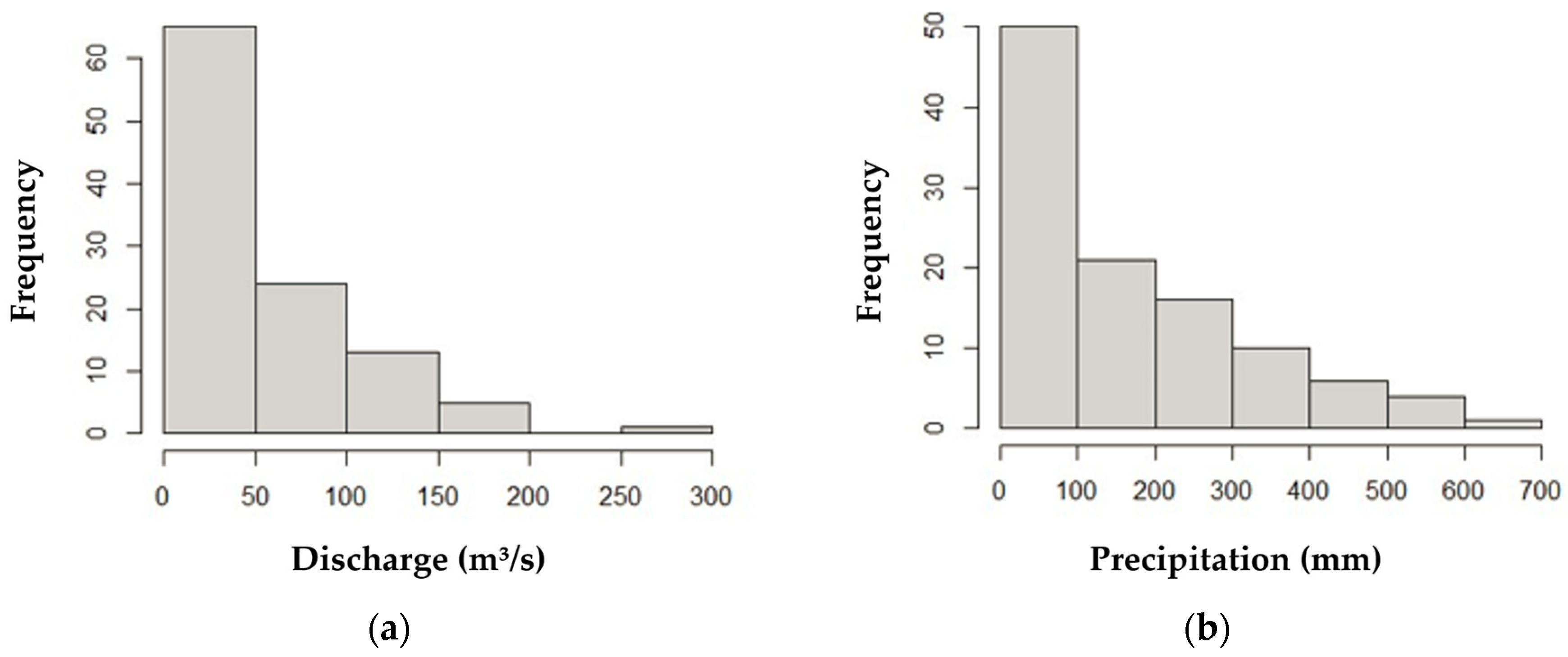
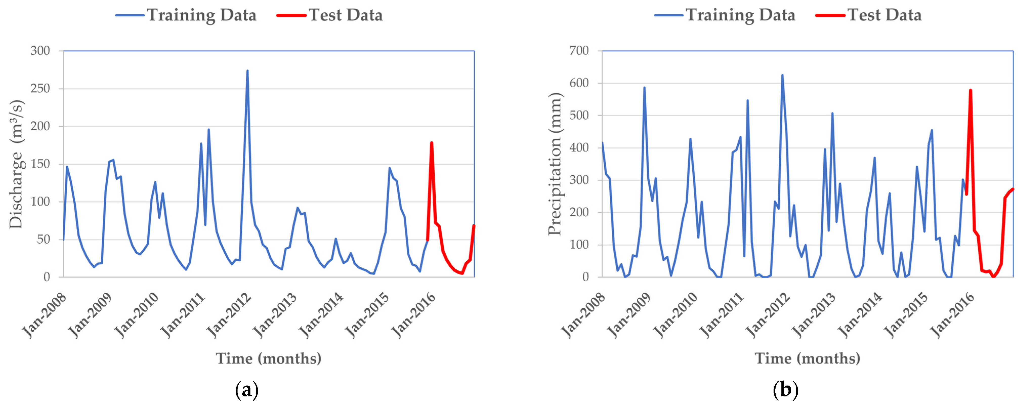
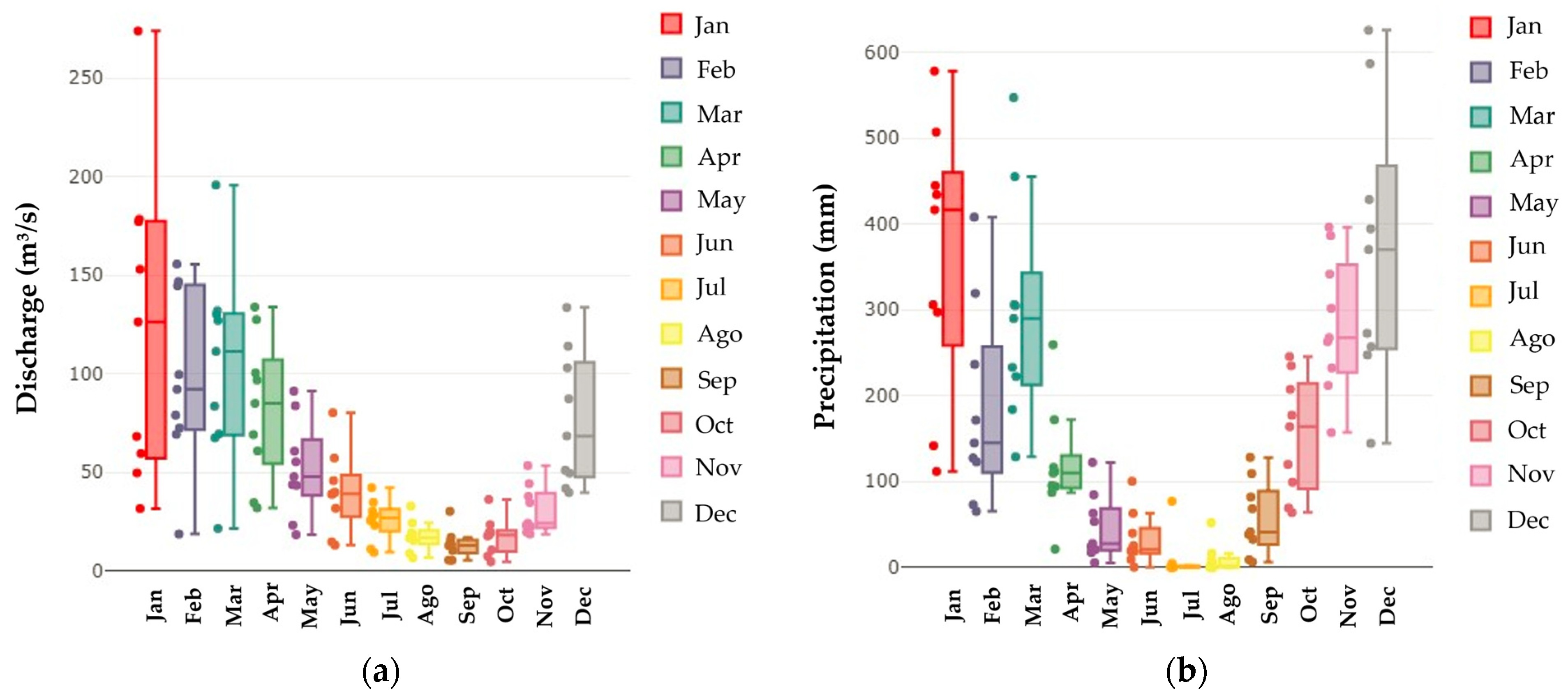
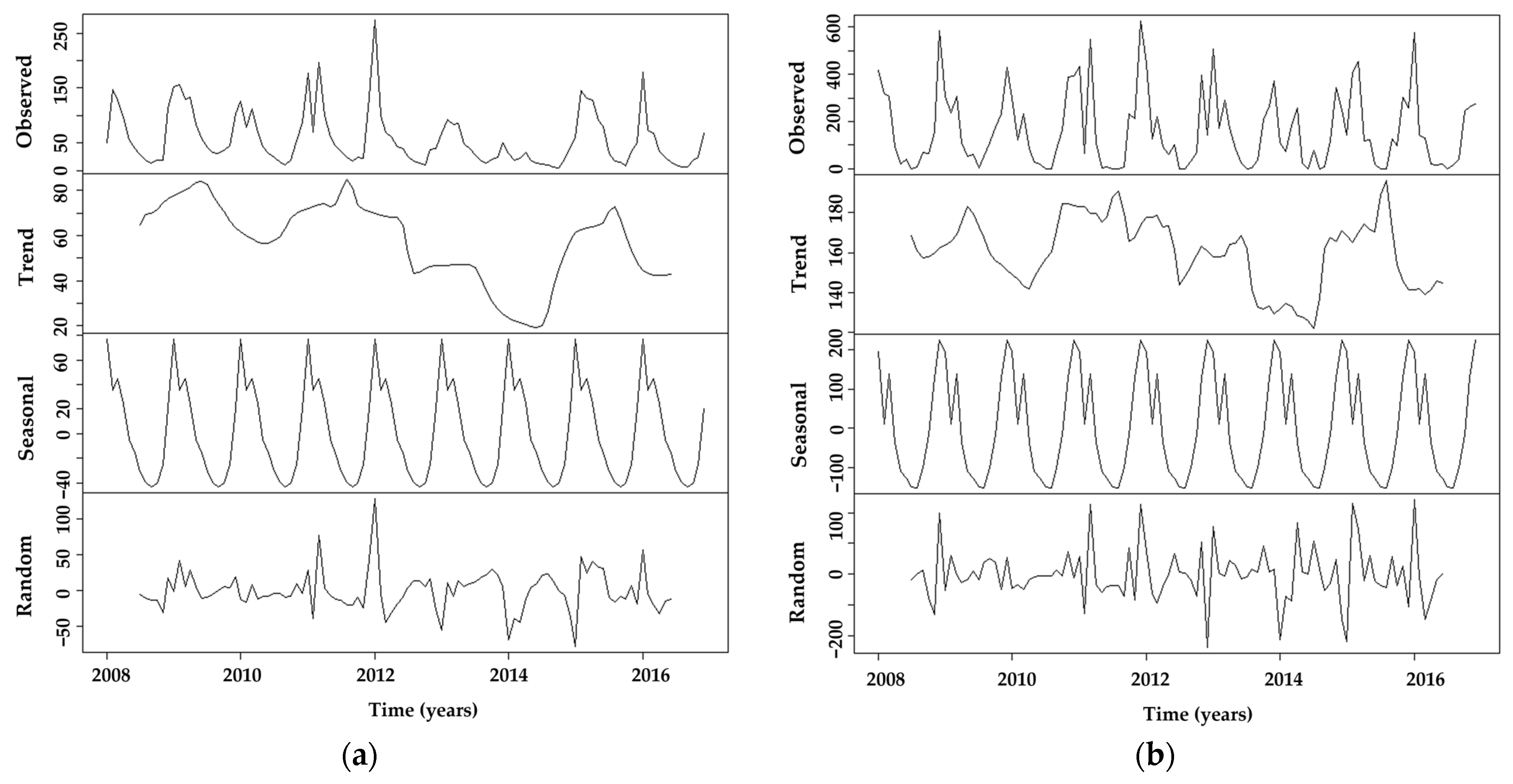
3.1. Statistical Analysis of Flow and Precipitation Data

The maximum discharge of 273.98 m³/s occurred in January 2012, while the minimum flow occurred in October 2014 with a value of 4.68 m³/s. High values for the standard deviation and coefficient of variation indicate that the arithmetic mean does not adequately represent the series. The highest recorded precipitation occurred in December 2011, reaching a value of 625.73 mm. Conversely, there were several dry months, especially during June, July, and August. The positive asymmetry reveals a higher concentration of low values in the sample [13], with further evidence in the histograms in Figure 2.

Figure 3a presents a line graph with the average monthly discharge time series and their division between the training and test periods. The flow series has a pattern of intra-annual variability, with periods of high discharges and floods followed by periods of drought, thus portraying the presence of seasonality [18,64]. Figure 3b displays a similar plot for the average monthly precipitation time series and its division between the training and testing periods, following guidelines in the literature [48,67].

Seasonality can be better visualized in the boxplots in Figure 4, exhibiting the seasonal pattern for the variables throughout the year based on the records from 2008 to 2016.

Figure 5 displays the monthly average discharge and precipitation time series, decomposed into trend, seasonality, and random components. In the seasonal component, it is evident that both series exhibit periodic oscillations around a mean value, confirming the presence of seasonality in the analyzed data. Such a pattern was expected because of the well-defined climatological behavior of this region, as described in Section 2.1, especially concerning precipitation. Conversely, the trend component does not exhibit discernible patterns in their decomposition. One may understand that the 9 year time series is insufficient to identify a markable trend cycle. However, the random component also did not show a pattern, and, as it is a remainder counterpart of the decomposition, this means it is a good indicator for ARIMA-type models and their variations, such as SARIMA and SARIMAX, which extract characteristics of the time series by stochastic processes.

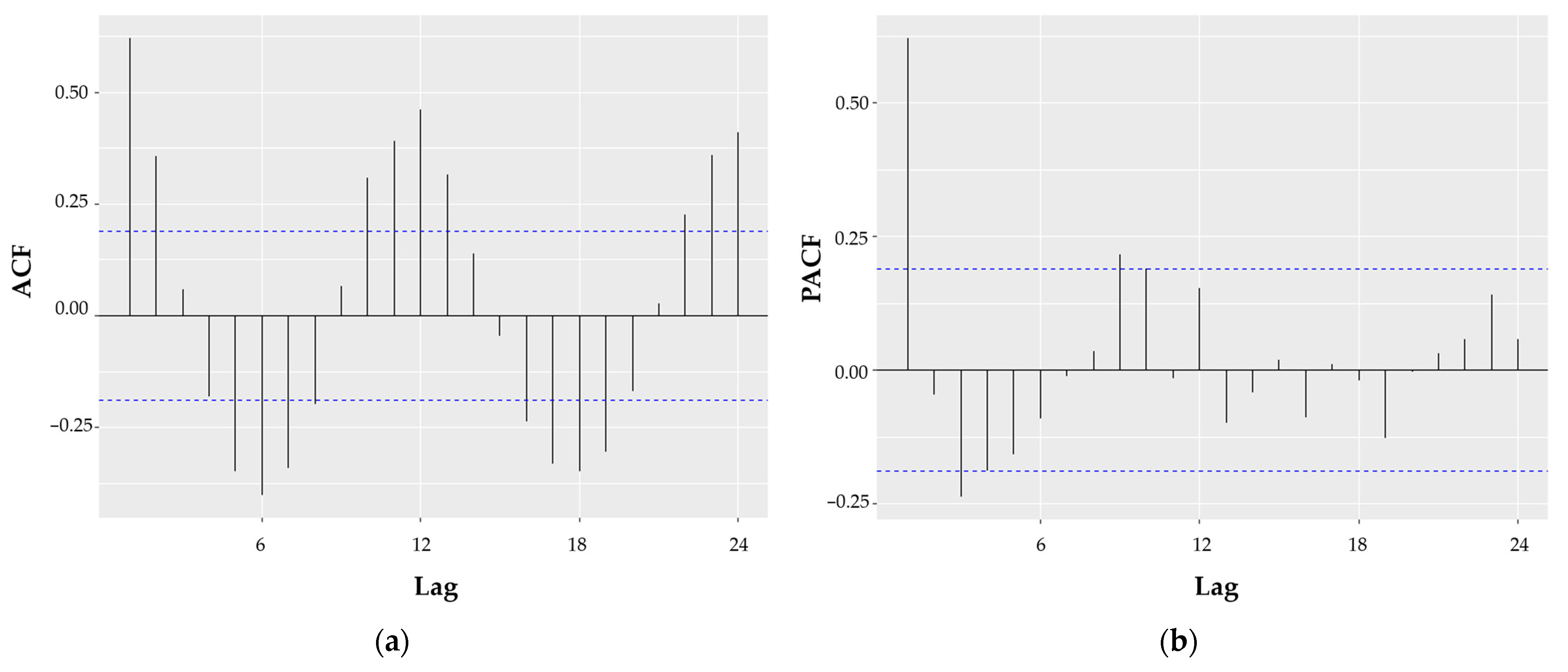
3.2. Model Identification

Analyzing the correlogram of the sample autocorrelation (ACF) and partial autocorrelation (PACF) functions plays a crucial role in model identification [17]. Figure 6 illustrates the ACF and PACF for the monthly average discharge data series. These correlograms show significant autocorrelation at multiple lags of 12, indicating the presence of seasonality. Consequently, the identification of a seasonal component is evident. Additionally, the sinusoidal and persistent behavior observed in the ACF correlogram suggests an autoregressive, non-stationary, and seasonal process.

The identification of the best-fit models was conducted with the aid of the “auto.arima()” function of the R package “forecast” [54], with the results indicating the selection of SARIMA (0,0,2)(0,1,1)₁₂ and SARIMAX (2,0,0)(2,1,0)₁₂. The SARIMA model presented an AIC of 855.34 and a BIC of 865.06, while the SARIMAX had an AIC of 831.49 and a BIC of 846.08. By analyzing these parameters comparatively, it is noticeable that the values of a SARIMA model decrease for a SARIMAX model.

The Bayesian information criterion (BIC) value tends to be higher for more complex models as it can measure a model’s complexity based on the number of parameters and the sample size [17,68]. Thus, simpler models have lower BIC values. When comparing the BIC values of the SARIMA and SARIMAX models, the results suggest a better performance of the SARIMAX model, which exhibited a lower BIC despite its higher complexity.

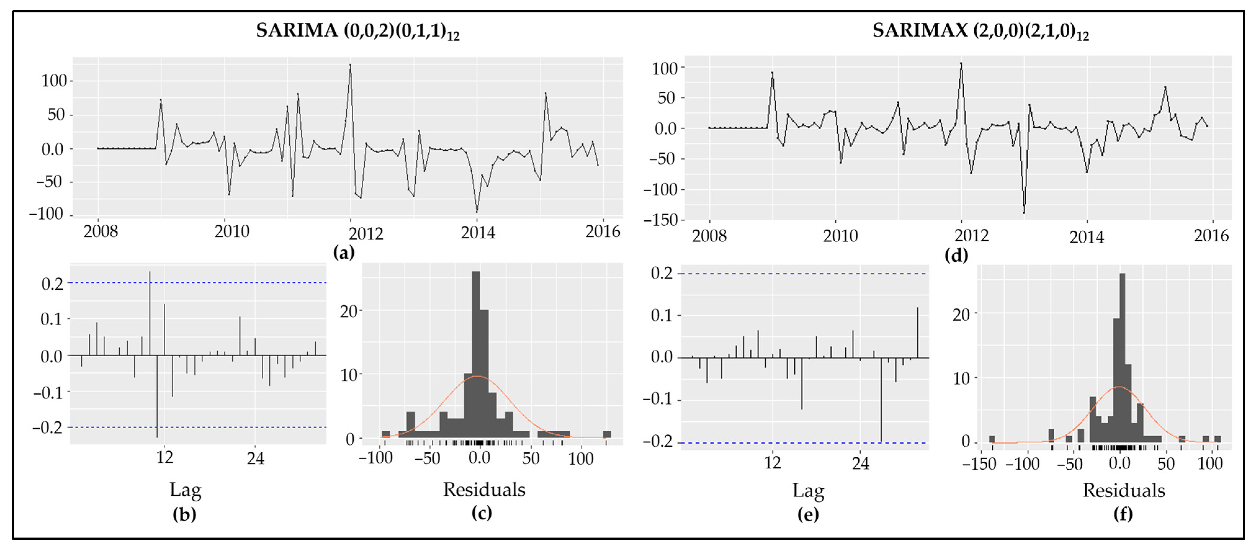
3.3. Diagnostic Analysis of the Models

The models’ residuals are expected to be random, uncorrelated, exhibit a normal distribution, and have a mean of zero [13,67]. The normality of the series was verified using the Shapiro–Wilk test according to the method described in [69], and the Ljung–Box test was used to assess the absence of correlation among the residuals, confirming white noise characteristics. The p-values of both tests suggest that the models exhibited a non-significant deviation from normality and uncorrelated residuals.

Figure 7 displays the residuals’ time series plots, correlograms, and histograms for both the SARIMA and SARIMAX models. The graphs of the SARIMA and SARIMAX models show that the residuals exhibit a normal distribution and lack correlation in both cases. The correlogram displays lags near zero, with only two values of the SARIMA model falling outside the significance range and none for the SARIMAX model, indicating that the residuals are uncorrelated and validating both models. However, the SARIMAX model performs better in the residual analysis, as all the lags are within the significance interval and are close to zero.

Figure 8 provides a comparison between the time series of observed average monthly discharges (dark line), the SARIMA model (red line), and the SARIMAX model (blue line) for the training period. During the first 12 months, the values are equal. Upon visual inspection of the graph, it is apparent that both training series follow the general behavior of the time series of records. Nevertheless, the values generated by the SARIMAX model are generally closer to extreme observations (minimum and maximum) and average values. Even if both models underestimate maxima, the plot shows that the SARIMA model tends to underestimate peaks by an average of 6.5% and overestimate troughs by approximately 76.0%. In contrast, the SARIMAX model overestimates the peaks by 11.6% and the troughs by around 5.0%. The models generally appear closer to capturing extreme peak events effectively, with SARIMA particularly overestimating troughs and SARIMAX providing a better fit overall for the extreme values.

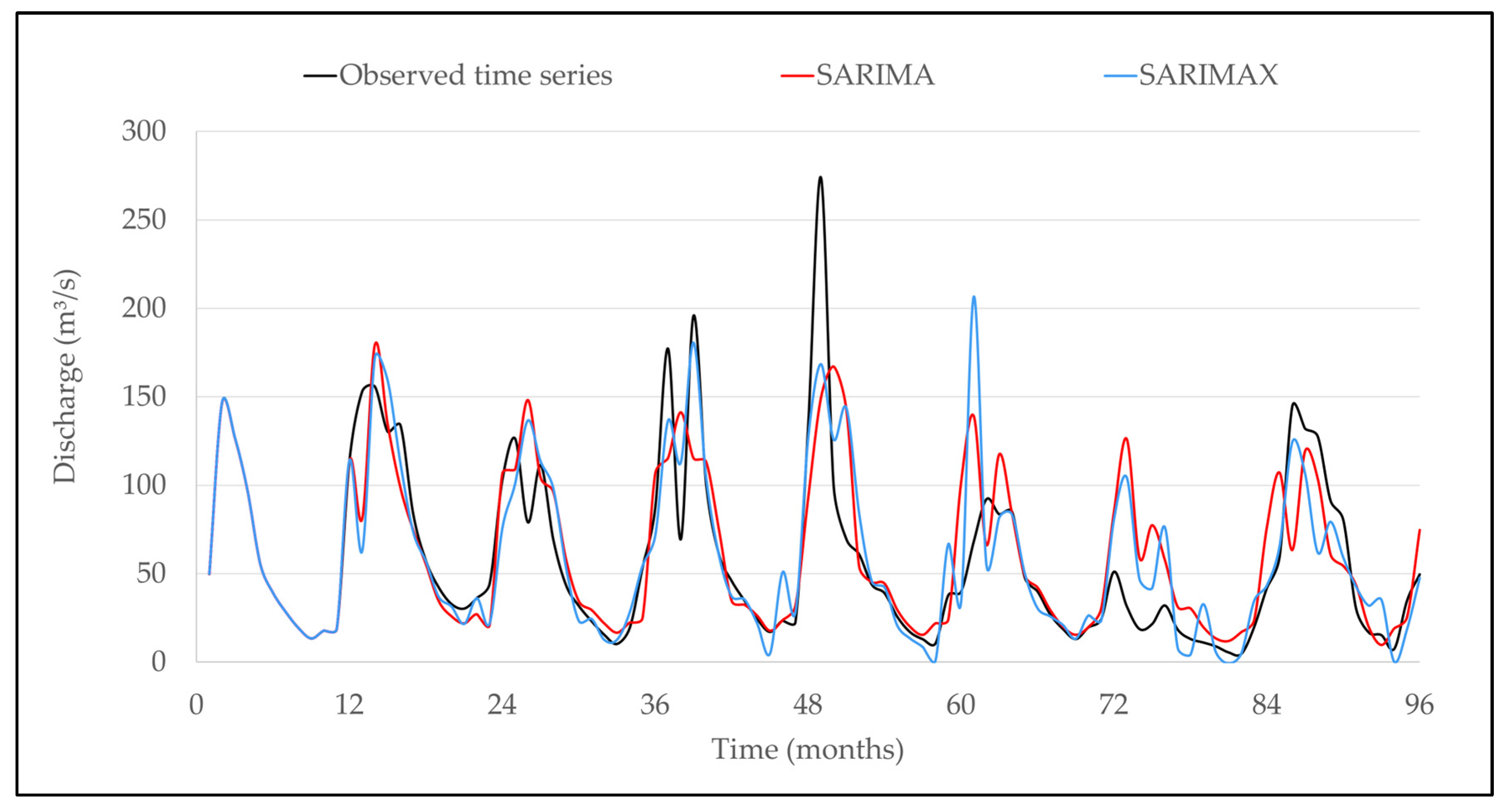
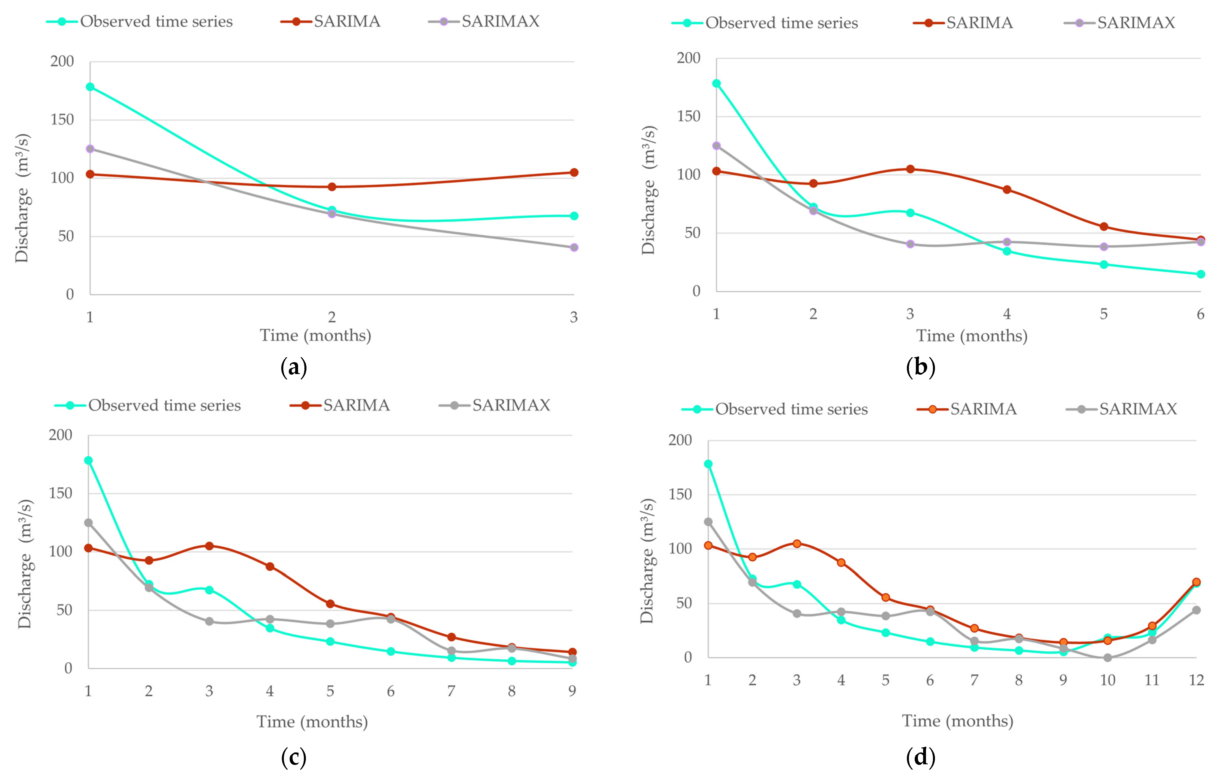
3.4. Forecasting Average Monthly Discharge

While this study primarily concentrates on monthly averages, the results in Figure 8 indicate that the minimum and most of the maximum values were adequately modeled. However, the highest value among the maximum discharge for the training period was not accurately represented. This discrepancy becomes evident when simulating the maximum values during the testing period, as illustrated in Figure 9. In this phase, forecasts of average monthly discharges are provided for horizons of three, six, nine, and twelve months (respectively, from Figure 9a to Figure 9d), corresponding to the year 2016. The predictions generated by the SARIMAX model align closer with the observed data across all forecast horizons.

Figure 9d presents the predicted and observed data for all of the months of 2016. The SARIMAX forecast was closer to the observations at 9 months, being less accurate than SARIMA in June, October, and December, and it is worth noting that, compared with SARIMAX, the forecast obtained by the SARIMA model for June produced a marginally more precise value.

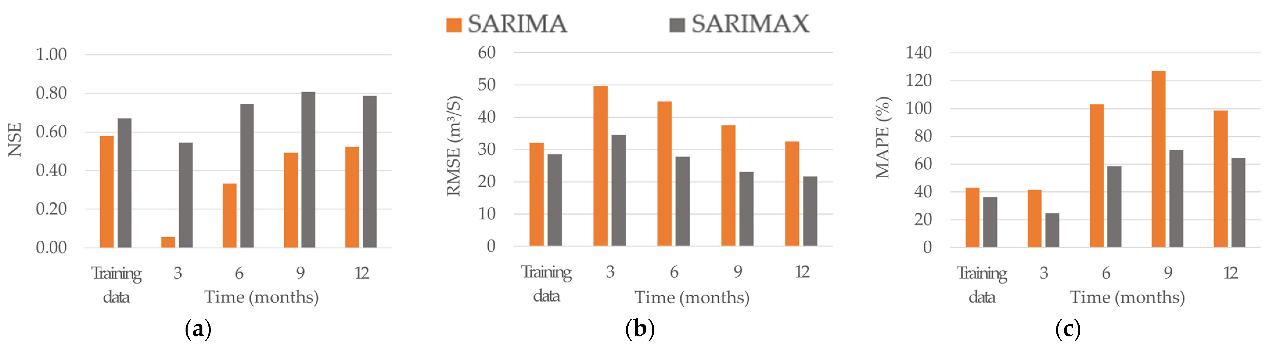
3.5. Performance Assessment of the Models

In order to assess the accuracy and precision of the proposed models, the NSE, RMSE, and MAPE performance metrics were calculated for the four forecast horizons, following the approach of Dazzi [58] and Pushpalatha et al. [59]. Figure 10 illustrates the NSE, RMSE, and MAPE performance metrics for the SARIMA and SARIMAX models.

The results demonstrate that the SARIMAX model outperforms the SARIMA model, with the NSE values obtained for the SARIMAX model falling into the classification of acceptability and good fit defined by Moriasi et al. [56]. Similarly, when considering the root mean square error (RMSE) and the absolute percentage error (MAPE), the values exhibited a substantial reduction, confirming that the incorporation of precipitation as an explanatory variable improved performance for the SARIMAX model.

Figure 10 suggests overfitting for the SARIMA model. This overfitting is apparent in the NSE and MAPE metrics when comparing the training and testing periods, in line with the observations of Hyndman and Athanasopoulos [48] and Chollet et al. [70]. The training phase exhibited a high value for the NSE metric but decreased significantly in all forecast horizons during testing. In contrast, the MAPE metric showed a noteworthy increase in the testing horizons compared with the training phase. Because the SARIMAX model does not exhibit this characteristic, these results indicate that the learning capacity of SARIMAX demonstrated a better fit than SARIMA.

4. Discussion

The time series analysis outcome heavily relies on the data series length, nature, and reliability, as these data serve as a crucial information source in subsequent statistical procedures. In this regard, even if a stochastic model is exceptionally well-designed, it cannot enhance the accuracy of parameters estimated from low-quality data. Therefore, hydrologists should evaluate the data’s quality before progressing to the subsequent stages of hydrological frequency analysis [13]. Stochastic validation assesses a model’s capability to replicate watershed response by converting the uncertainty associated with model parameters into predictive uncertainty by utilizing probability distribution functions for these parameters [14].

It is worth noting that models can have short-term and long-term predictive capabilities, with this study focusing on long-term predictions in line with the definitions of Mosavi et al. [71]. The observed errors suggest that SARIMA models tend to be more reliable for longer-term forecasts, in line with the findings of Alonso Brito et al. [72]. Additionally, the performance of SARIMA models is highly sensitive to the training time series used in model calibration, as highlighted by Danandeh Mehr et al. [35].

Regarding the challenges and limitations associated with the use of stochastic models for discharge forecasting in regions facing severe water crises or frequent floods, one major issue is the consideration of time series stationarity. This aspect can introduce uncertainties, as the time series of the variable or variables under consideration might exhibit pattern changes over time due to climate change, deforestation, land use, or land cover changes, among other factors [73,74]. In addition to stationarity, another source of inaccuracies is the assumption of a linear or pseudo-linear relationship between the explanatory variables (exogenous) and the target variable (target), which may not be accurate in some hydrological systems [75]. Nevertheless, both issues can be addressed. Non-stationary time series can be transformed into stationary ones through mathematical transformations (e.g., logarithmic, exponential) [48], and using ANN is an effective approach for dealing with the assumption of linearity in hydrological systems when this is not valid [5].

The NSE coefficient values of this study indicate that the SARIMAX model consistently outperformed the SARIMA model, with results ranging from satisfactory to very good across all time horizons under consideration [56]. In contrast, the SARIMA model only achieved a satisfactory rating at the 12 month forecast horizon. For instance, these findings differ from those of Danandeh Mehr et al. [35,76] in their studies conducted for rivers in Turkey and Finland, whose NSE results with the SARIMA model report inferior to satisfactory performance in long-term forecasting. Similarly, the research of Chechi and Sanches [37] and Meis et al. [77] observed the improved performance of SARIMAX to SARIMA in their studies for Brazilian watersheds, with their analyses highlighting the model’s strengths in metrics like RMSE, NSE, and R².

As observed in studies for various Brazilian watersheds, including explanatory variables in the SARIMA model (resulting in SARIMAX models) usually leads to improvements in the accuracy of these forecasting tools [23,36,37,38,39], as is the case in this article. Recent studies worldwide also support this hydrological research topic. One example is the paper by Harat and Zarch [78], which demonstrated improved results in long-duration drought prediction by adding precipitation and evapotranspiration (separately) as exogenous variables in the SARIMAX model. Another common approach in the literature, instead of directly forecasting flow rates, is configuring time series models of precipitation and temperature and using these products in hydrological models to obtain estimates of discharge time series [69,79,80].

Forecasting extreme hydrological events is particularly important in a changing climate [51], posing challenges for stochastic hydrological models in the accurate representation of such events, with most studies reporting limited satisfactory results. For example, Danandeh Mehr et al. [76] encountered considerable inaccuracies when modeling drier months, a similarity also observed in this research as well as in other previous studies in Brazil [23,38,39]. Additionally, models tend to underestimate peak discharge, and, while this was true for the test period of this research, the training period exhibited mixed results. Possible reasons for these variations between observed values and model estimations include the anomalous year 2014, the most severe drought in the region in decades [81], water withdrawal during the dry season, and the influence of ENSO [37].

Kim et al. [82] utilized SARIMA and SARIMAX models for forecasting reservoir inflows within the Han River basin, South Korea. They used prior streamflow as an autoregressive variable and climate indices as exogenous variables. However, including climatic variables did not significantly improve prediction outcomes, and these SARIMA and SARIMAX models could not forecast high streamflow periods. Following a similar methodology, Meis et al. [83] included a forecast based on the ENSO 3.4 index to configure a SARIMAX model with which to forecast extreme discharge events in the La Plata basin, outperforming a SARIMA model for discharge predictions horizons of 6 months and 12 months during El Niño events. This approach allowed for a satisfactory prediction of extreme floods, suggesting its potential for future research in the study area of the present paper. Another relatively underexplored area is the integration of ARIMA family models with artificial neural network (ANN) models in hybrid modeling. For instance, Khairuddin et al. [5] compared various time series analysis techniques for a watershed in Malaysia, including linear regression, ARIMA, and ANN. In their study of real-time flood prediction based on precipitation and water level data, these authors found that ANN outperformed the other methods, aligning with the results reported by Kim et al. [82]. In this context, employing SARIMAX models as tools for hydrological forecasting and water resource management in urban areas offers the potential for the inclusion of predictor (exogenous) variables related to urbanization, such as the evolution of impervious surface percentages or the consideration of water levels in urban channels in stochastic modeling.

For urban areas in particular, non-structural measures such as hydrological forecasting, flood emergency response plans, and post-flood recovery guidelines and actions represent solid and cost-effective alternatives to structural solutions in flood management [84]. Furthermore, activities such as the conversion of native forest or pasture to agriculture or impervious urban areas can increase areas prone to flooding, as evidenced by Houspanossian et al. [85] in South America. Human activities notably influence the variability of hydrological time series. Wu et al. [86] presented a SARIMA-GARCH adaptation, which considers the impact of human activities and natural stressors in the volatility of a karst spring discharge in China, aiming to improve water resource management in regions influenced by anthropogenic activities.

As frequently occurs in developing countries [32,87], the main limitation of the present study was the relatively short time series of measurements available to conduct this research. Therefore, future and similar studies could benefit from longer time series encompassing flood and drought periods in their training and testing periods, aiming to improve the understanding and forecasting of extreme values. Additionally, although the models used are naturally stochastic, they produce deterministic outputs. Hence, the authors strongly recommend including model uncertainty analysis to enable the stochastic use of model responses.

In developing countries like Brazil, several areas need flow monitoring and forecasting for both maximum and minimum extremes, and in general, they need more monitoring data and personnel available to develop more detailed physical models. Still, available resources for this purpose are commonly scarce or insufficient, even more so considering the extension of this country. Nevertheless, in the meantime, reducing the risks to human populations in basins with limited data is necessary, thus justifying the development of models that require less input data, such as in the approach of this study.

Despite these limitations, the results of this research hold significance from an urban perspective, particularly for the population in the study area. The Paranaíba River is the primary water supply source of, and receives sewage discharge from, the population in Patos de Minas [40]. In the context of climate change, some projections estimate a decrease in extreme precipitations and flood events in the region [88], emphasizing the importance of long-term flow predictions that use these models to assist in efficient resource management, ensuring a continuous water supply and helping mitigate risks associated with urban activities and expansion. Future studies may integrate additional approaches, for instance, to include short-term daily predictions, as in Meis et al. [77], to explore extreme scenarios under the influence of climate change [89] or to assess the impact of anthropogenic effects on water quality parameters [90].

5. Conclusions

This article investigates the applicability of ARIMA class models for long-term discharge forecasts in the Paranaíba River basin, a vital water source and a recipient of urban sewage discharge in Patos de Minas, features that make it an illustrative case study of urban areas facing similar challenges. This study configured and compared two stochastic models for predicting monthly average discharge in a Paranaíba River sub-basin in Patos de Minas, MG, Brazil. The first selected model was SARIMA (0,0,2)(0,1,1)₁₂, which accounts for seasonality in the series. The second seasonal model was the SARIMAX (2,0,0)(2,1,0)₁₂, which includes precipitation as a regressor variable. The AIC and BIC criteria were used for automatic model selection, resulting in a better fit for the SARIMAX model than the SARIMA model.

According to the diagnostic phase of the models, the SARIMAX model outperformed SARIMA in terms of residual analysis and when evaluating performance metrics such as NSE, RSME, and MAPE. Thus, precipitation as a regressor variable in the monthly average flow prediction model substantially improved forecasting performance for this study. This improvement can be attributed to the multivariate structure of the SARIMAX model.

The practical implications of this research extend to supporting decision-making processes within public agencies, particularly environmental departments. SARIMAX models are helpful and cost-effective tools for decision processes related to defining strategic priorities and the effective and sustainable management of water resources within river basins.

While this study focused on monthly average flow predictions, future research endeavors could explore shorter-term daily predictions, particularly in light of extreme event forecasting. Moreover, there is an opportunity to investigate the influence of climate change and anthropogenic factors on water quality parameters, expanding the scope of applications for SARIMAX models in urban water resource management.

Given climate change projections highlighting the significance of long-term flow predictions for resource management and risk mitigation in human communities, especially for growing urban areas, the findings of this study hold practical relevance. Furthermore, this study’s approach of applying ARIMA models for long-term discharge forecasts in an area confronting similar urban challenges underscores its importance as an illustrative case study. Therefore, the presented method is a promising tool for enhancing the accuracy of urban hydrodynamic modeling and forecasting, thereby contributing to making cities more resilient to floods.

References

1. Patel, S.S.; Ramachandran, P. A Comparison of Machine Learning Techniques for Modeling River Flow Time Series: The Case of Upper Cauvery River Basin. Water Resour. Manag. 2015, 29, 589–602. [Google Scholar] [CrossRef]
2. Ehteram, M.; Afan, H.A.; Dianatikhah, M.; Ahmed, A.N.; Ming Fai, C.; Hossain, M.S.; Allawi, M.F.; Elshafie, A. Assessing the Predictability of an Improved ANFIS Model for Monthly Streamflow Using Lagged Climate Indices as Predictors. Water 2019, 11, 1130. [Google Scholar] [CrossRef]
3. Höge, M.; Scheidegger, A.; Baity-Jesi, M.; Albert, C.; Fenicia, F. Improving Hydrologic Models for Predictions and Process Understanding Using Neural ODEs. Hydrol. Earth Syst. Sci. 2022, 26, 5085–5102. [Google Scholar] [CrossRef]
4. Tolentino, A.H.A.; Vieira, E.D.O.; Rezende, B.N.; Amaral, P.A.A.; Frazão, L.A. Soil loss in the São Lamberto river basin with use of temporary series of Landsat. Agrarian 2020, 13, 362–376. [Google Scholar] [CrossRef]
5. Khairuddin, N.; Aris, A.Z.; Elshafie, A.; Sheikhy Narany, T.; Ishak, M.Y.; Isa, N.M. Efficient Forecasting Model Technique for River Stream Flow in Tropical Environment. Urban Water J. 2019, 16, 183–192. [Google Scholar] [CrossRef]
6. Devi, G.K.; Ganasri, B.P.; Dwarakish, G.S. A Review on Hydrological Models. Aquat. Procedia 2015, 4, 1001–1007. [Google Scholar] [CrossRef]
7. Pandi, D.; Kothandaraman, S.; Kuppusamy, M. Hydrological Models: A Review. Int. J. Hydrol. Sci. Technol. 2021, 12, 223. [Google Scholar] [CrossRef]
8. Wagena, M.B.; Goering, D.; Collick, A.S.; Bock, E.; Fuka, D.R.; Buda, A.; Easton, Z.M. Comparison of Short-Term Streamflow Forecasting Using Stochastic Time Series, Neural Networks, Process-Based, and Bayesian Models. Environ. Model. Softw. 2020, 126, 104669. [Google Scholar] [CrossRef]
9. Ng, K.W.; Huang, Y.F.; Koo, C.H.; Chong, K.L.; El-Shafie, A.; Najah Ahmed, A. A Review of Hybrid Deep Learning Applications for Streamflow Forecasting. J. Hydrol. 2023, 625, 130141. [Google Scholar] [CrossRef]
10. Jehanzaib, M.; Ajmal, M.; Achite, M.; Kim, T.-W. Comprehensive Review: Advancements in Rainfall-Runoff Modelling for Flood Mitigation. Climate 2022, 10, 147. [Google Scholar] [CrossRef]
11. Sharma, P.; Machiwal, D. Streamflow Forecasting. In Advances in Streamflow Forecasting. From Traditional to Modern Approaches; Elsevier: Amsterdam, The Netherlands, 2021; pp. 1–50. ISBN 978-0-12-820673-7. [Google Scholar]
12. Kilinc, H.C.; Yurtsever, A. Short-Term Streamflow Forecasting Using Hybrid Deep Learning Model Based on Grey Wolf Algorithm for Hydrological Time Series. Sustainability 2022, 14, 3352. [Google Scholar] [CrossRef]
13. Naghettini, M. (Ed.) Fundamentals of Statistical Hydrology; Springer International Publishing: Cham, Switzerland, 2017; ISBN 978-3-319-43560-2. [Google Scholar]
14. Cibin, R.; Athira, P.; Sudheer, K.P.; Chaubey, I. Application of Distributed Hydrological Models for Predictions in Ungauged Basins: A Method to Quantify Predictive Uncertainty. Hydrol. Process. 2014, 28, 2033–2045. [Google Scholar] [CrossRef]
15. Vogel, R.M. Stochastic Watershed Models for Hydrologic Risk Management. Water Secur. 2017, 1, 28–35. [Google Scholar] [CrossRef]
16. Larsen, S.; Karaus, U.; Claret, C.; Sporka, F.; Hamerlík, L.; Tockner, K. Flooding and Hydrologic Connectivity Modulate Community Assembly in a Dynamic River-Floodplain Ecosystem. PLoS ONE 2019, 14, e0213227. [Google Scholar] [CrossRef] [PubMed]
17. Machiwal, D.; Jha, M.K. Hydrologic Time Series Analysis: Theory and Practice; Springer Netherlands: Dordrecht, The Netherlands, 2012; ISBN 978-94-007-1860-9. [Google Scholar]
18. Maçaira, P.M.; Tavares Thomé, A.M.; Cyrino Oliveira, F.L.; Carvalho Ferrer, A.L. Time Series Analysis with Explanatory Variables: A Systematic Literature Review. Environ. Model. Softw. 2018, 107, 199–209. [Google Scholar] [CrossRef]
19. Box, G.E.P.; Jenkins, G.M. Time Series Analysis, Forecasting and Control; Holden-Day: San Francisco, CA, USA, 1976. [Google Scholar]
20. Bayer, F.M.; Souza, A.M. Forecasting with Wavelets and Traditional Models: A Comparative. Rev. Bras. Biom. 2010, 28, 40–61. [Google Scholar]
21. Vagropoulos, S.I.; Chouliaras, G.I.; Kardakos, E.G.; Simoglou, C.K.; Bakirtzis, A.G. Comparison of SARIMAX, SARIMA, Modified SARIMA and ANN-Based Models for Short-Term PV Generation Forecasting. In Proceedings of the 2016 IEEE International Energy Conference and Exhibition, Leuven, Belgium, 4–8 April 2016; pp. 1–6. [Google Scholar] [CrossRef]
22. Adnan, R.M.; Yuan, X.; Kisi, O.; Yuan, Y.; Tayyab, M.; Lei, X. Application of Soft Computing Models in Streamflow Forecasting. Proc. Inst. Civ. Eng. Water Manag. 2019, 172, 123–134. [Google Scholar] [CrossRef]
23. Bleidorn, M.T.; Pinto, W.D.P.; Braum, E.S.; Lima, G.B.; Montebeller, C.A. Modelling and Prevision of Monthly Mean Flow of Jucu River, ES, Using SARIMA Model. IRRIGA 2019, 24, 320–335. [Google Scholar] [CrossRef]
24. Farjalla, V.F.; Pires, A.P.F.; Agostinho, A.A.; Amado, A.M.; Bozelli, R.L.; Dias, B.F.S.; Dib, V.; Faria, B.M.; Figueiredo, A.; Gomes, E.A.T.; et al. Turning Water Abundance into Sustainability in Brazil. Front. Environ. Sci. 2021, 9, 1–12. [Google Scholar] [CrossRef]
25. ANA—Agência Nacional de Águas e Saneamento Básico Conjuntura Dos Recursos Hídricos No Brasil. 2021. Available online: https://relatorio-conjuntura-ana-2021.webflow.io/ (accessed on 15 August 2022).
26. Gordy, M. Disaster Risk Reduction and the Global System; SpringerBriefs in Climate Studies; Springer International Publishing: Cham, Switzerland, 2016; ISBN 978-3-319-41666-3. [Google Scholar]
27. Intergovernmental Panel on Climate Change. Climate Change 2021—The Physical Science Basis; Masson-Delmotte, V., Zhai, P., Pirani, A., Connors, S.L., Péan, C., Berger, S., Caud, N., Chen, Y., Goldfarb, L., Gomis, M.I., et al., Eds.; Cambridge University Press: New York, NY, USA, 2023; ISBN 9781009157896. [Google Scholar]
28. Lyra, A.; Tavares, P.; Chou, S.C.; Sueiro, G.; Dereczynski, C.; Sondermann, M.; Silva, A.; Marengo, J.; Giarolla, A. Climate Change Projections over Three Metropolitan Regions in Southeast Brazil Using the Non-Hydrostatic Eta Regional Climate Model at 5-Km Resolution. Theor. Appl. Climatol. 2018, 132, 663–682. [Google Scholar] [CrossRef]
29. Chou, S.C.; Lyra, A.; Mourão, C.; Dereczynski, C.; Pilotto, I.; Gomes, J.; Bustamante, J.; Tavares, P.; Silva, A.; Rodrigues, D.; et al. Assessment of Climate Change over South America under RCP 4.5 and 8.5 Downscaling Scenarios. Am. J. Clim. Chang. 2014, 3, 512–527. [Google Scholar] [CrossRef]
30. Towner, J.; Cloke, H.L.; Lavado, W.; Santini, W.; Bazo, J.; Coughlan de Perez, E.; Stephens, E.M. Attribution of Amazon Floods to Modes of Climate Variability: A Review. Meteorol. Appl. 2020, 27, e1949. [Google Scholar] [CrossRef]
31. Souza, F.A.A.D.; Mendiondo, E.M.; Taffarello, D.; Guzmán-Arias, D.; Fava, M.C.; Abreu, F.; Freitas, C.C.; de Macedo, M.B.; Estrada, C.R.; do Lago, C.A. Socio-Hydrological Observatory for Water Security (SHOWS): Examples of Adaptation Strategies with Next Challenges from Brazilian Risk Areas. In Proceedings of the AGU Fall Meeting Abstracts, New Orleans, LA, USA, 11–15 December 2017; Volume 2017, p. H13S-08. [Google Scholar]
32. Centro Nacional de Monitoramento e Alertas de Desastres Naturais. Anuário Da Sala de Situação Do CEMADEN, 2017; CEMADEN: São José dos Campos, Brazil, 2019. [Google Scholar]
33. Kassem, A.A.; Raheem, A.M.; Khidir, K.M. Daily Streamflow Prediction for Khazir River Basin Using ARIMA and ANN Models. Zanco J. Pure Appl. Sci. 2020, 32, 30–39. [Google Scholar] [CrossRef]
34. Sun, Y.; Niu, J.; Sivakumar, B. A Comparative Study of Models for Short-Term Streamflow Forecasting with Emphasis on Wavelet-Based Approach. Stoch. Environ. Res. Risk Assess. 2019, 33, 1875–1891. [Google Scholar] [CrossRef]
35. Danandeh Mehr, A.; Ghadimi, S.; Marttila, H.; Torabi Haghighi, A. A New Evolutionary Time Series Model for Streamflow Forecasting in Boreal Lake-River Systems. Theor. Appl. Climatol. 2022, 148, 255–268. [Google Scholar] [CrossRef]
36. Bayer, D.; Castro, N.; Bayer, F. Modeling and forecasting mean monthly streamflows using time series. Rev. Bras. Recur. Hídricos 2012, 17, 229–239. [Google Scholar] [CrossRef]
37. Chechi, L.; Sanches, F. de O. Analysis of a Series of Precipitation for Erechim (RS) and a Method of Possible Climate Prediction. Rev. Ambiência 2013, 9, 43–55. [Google Scholar] [CrossRef]
38. Pinto, W.D.P.; Lima, G.B.; Zanetti, J.B. Comparative Analysis of Models for Times to Series Modeling and Forecasting of Scheme of Average Monthly Streamflow of the Doce River, Colatina Espirito Santo, Brazil. Ciência Nat. 2015, 37, 1–11. [Google Scholar] [CrossRef]
39. Caixeta, L.T.; de Menezes Filho, F.C.M.; Fonseca, V.L.A. Modeling and forecasting mean monthly streamflows of Paranaiba River using SARIMA model. Rev. Ibero-Am. Ciências Ambient. 2021, 12, 255–267. [Google Scholar] [CrossRef]
40. da Silva, L.L.; Goulart, A.T.; de Melo, C.; de Oliveira, R.d.C.W. Microbiological, Chemical and Physical-Chemical Assessment of the Contamination in the Paranaíba River. Soc. Nat. 2006, 18, 45–62. [Google Scholar] [CrossRef]
41. ANA—Agência Nacional de Águas e Saneamento Básico HIDROWEB. Available online: https://www.snirh.gov.br/hidroweb/apresentacao (accessed on 15 September 2022).
42. IBGE—Instituto Brasileiro de Geografia e Estatística Portal Cidades. Available online: https://www.ibge.gov.br/cidades-e-estados/mg/patos-de-minas.html (accessed on 15 September 2023).
43. Mendonça, F.; Danni-Oliveira, I.M. Climatologia: Noções Básicas e Climas Do Brasil; Oficina de Textos: São Paulo, Brazil, 2007. [Google Scholar]
44. Martins, F.B.; Gonzaga, G.; Dos Santos, D.F.; Reboita, M.S. Climate classification of Köppen and Thornthwaite for Minas Gerais: Crrent climate and climate changes. Rev. Bras. Climatol. 2018, 14, 129–156. [Google Scholar] [CrossRef]
45. de Oliveira, N.M.; Ribeiro, K.L.N.; Pereira, S.G.; Vieira, S.M. Milk Quality Assessment of Properties in the City of Patos de Minas, MG. Rev. Multidiscip. 2020, 23, 279–301. [Google Scholar]
46. Caixeta, C.L.B.; Piccinato Junior, D. Territory, Urbanity and Sustainability: A Study about the Recovery of Springs in a Rural Community in Patos de Minas/MG. Rev. Arquitetura IMED 2021, 10, 48–62. [Google Scholar] [CrossRef]
47. Federação das Indústrias do Estado do Rio de Janeiro IFDM. Índice FIRJAN de Desenvolvimento Municipal: Consulta. Available online: https://www.firjan.com.br/ifdm/ (accessed on 15 September 2023).
48. Hyndman, R.J.; Athanasopoulos, G. Forecasting: Principles and Practice, 3rd ed.; OTexts: Melbourne, VIC, Australia, 2021; ISBN 978-0987507136. [Google Scholar]
49. Alharbi, F.R.; Csala, D. A Seasonal Autoregressive Integrated Moving Average with Exogenous Factors (SARIMAX) Forecasting Model-Based Time Series Approach. Inventions 2022, 7, 94. [Google Scholar] [CrossRef]
50. Fazla, A.; Aydin, M.E.; Kozat, S.S. Joint Optimization of Linear and Nonlinear Models for Sequential Regression. Digit. Signal Process. 2023, 132, 103802. [Google Scholar] [CrossRef]
51. Oikonomou, P.D.; Alzraiee, A.H.; Karavitis, C.A.; Waskom, R.M. A Novel Framework for Filling Data Gaps in Groundwater Level Observations. Adv. Water Resour. 2018, 119, 111–124. [Google Scholar] [CrossRef]
52. Hyndman, R.J. Discussion of “High-Dimensional Autocovariance Matrices and Optimal Linear Prediction”. Electron. J. Stat. 2015, 9, 792–796. [Google Scholar] [CrossRef]
53. Morettin, P.A. The Levinson Algorithm and Its Applications in Time Series Analysis. Int. Stat. Rev. 1984, 52, 83–92. [Google Scholar] [CrossRef]
54. Hyndman, R.; Athanasopoulos, G.; Bergmeir, C.; Caceres, G.; Chhay, L.; Kuroptev, K.; O’Hara-Wild, M.; Petropoulos, F.; Razbash, S.; Wang, E.; et al. CRAN—Package Forecast. Available online: https://cran.r-project.org/web/packages/forecast/ (accessed on 18 September 2022).
55. Chakrabarti, A.; Ghosh, J.K. AIC, BIC and Recent Advances in Model Selection. In Philosophy of Statistics; Bandyopadhyay, P.S., Forster, M.R., Eds.; Elsevier: Amsterdam, The Netherlands, 2011; pp. 583–605. [Google Scholar]
56. Moriasi, D.N.; Arnold, J.G.; Van Liew, M.W.; Bingner, R.L.; Harmel, R.D.; Veith, T.L. Model Evaluation Guidelines for Systematic Quantification of Accuracy in Watershed Simulations. Trans. ASABE 2007, 50, 885–900. [Google Scholar] [CrossRef]
57. Kim, S.; Kim, H. A New Metric of Absolute Percentage Error for Intermittent Demand Forecasts. Int. J. Forecast. 2016, 32, 669–679. [Google Scholar] [CrossRef]
58. Dazzi, S.; Vacondio, R.; Mignosa, P. Flood Stage Forecasting Using Machine-Learning Methods: A Case Study on the Parma River (Italy). Water 2021, 13, 1612. [Google Scholar] [CrossRef]
59. Pushpalatha, R.; Perrin, C.; Le Moine, N.; Andréassian, V. A Review of Efficiency Criteria Suitable for Evaluating Low-Flow Simulations. J. Hydrol. 2012, 420–421, 171–182. [Google Scholar] [CrossRef]
60. Moriasi, D.N.; Gitau, M.W.; Pai, N.; Daggupati, P. Hydrologic and Water Quality Models: Performance Measures and Evaluation Criteria. Trans. ASABE 2015, 58, 1763–1785. [Google Scholar] [CrossRef]
61. Legates, D.R.; McCabe, G.J. Evaluating the Use of “Goodness-of-fit” Measures in Hydrologic and Hydroclimatic Model Validation. Water Resour. Res. 1999, 35, 233–241. [Google Scholar] [CrossRef]
62. Harmel, R.D.; Smith, P.K. Consideration of Measurement Uncertainty in the Evaluation of Goodness-of-Fit in Hydrologic and Water Quality Modeling. J. Hydrol. 2007, 337, 326–336. [Google Scholar] [CrossRef]
63. Harmel, R.D.; Smith, P.K.; Migliaccio, K.W. Modifying Goodness-of-Fit Indicators to Incorporate Both Measurement and Model Uncertainty in Model Calibration and Validation. Trans. ASABE 2010, 53, 55–63. [Google Scholar] [CrossRef]
64. Pant, J.; Sharma, R.K.; Juyal, A.; Singh, D.; Pant, H.; Pant, P. A Machine-Learning Approach to Time Series Forecasting of Temperature. In Proceedings of the 6th International Conference on Electronics, Communication and Aerospace Technology, Coimbatore, India, 1–3 December 2022; pp. 1125–1129. [Google Scholar] [CrossRef]
65. Hyndman, R.J.; Khandakar, Y. Automatic Time Series Forecasting: The Forecast Package for R. J. Stat. Softw. 2008, 27, 1–22. [Google Scholar] [CrossRef]
66. Lee, J.; Cho, Y. National-Scale Electricity Peak Load Forecasting: Traditional, Machine Learning, or Hybrid Model? Energy 2022, 239, 122366. [Google Scholar] [CrossRef]
67. Jain, S.K.; Mani, P.; Jain, S.K.; Prakash, P.; Singh, V.P.; Tullos, D.; Kumar, S.; Agarwal, S.P.; Dimri, A.P. A Brief Review of Flood Forecasting Techniques and Their Applications. Int. J. River Basin Manag. 2018, 16, 329–344. [Google Scholar] [CrossRef]
68. Konishi, S.; Kitagawa, G. Information Criteria and Statistical Modeling; Springer Series in Statistics; Springer: New York, NY, USA, 2008; Volume 27, ISBN 978-0-387-71886-6. [Google Scholar]
69. Martínez-Acosta, L.; Medrano-Barboza, J.P.; López-Ramos, Á.; Remolina López, J.F.; López-Lambraño, Á.A. SARIMA Approach to Generating Synthetic Monthly Rainfall in the Sinú River Watershed in Colombia. Atmosphere 2020, 11, 602. [Google Scholar] [CrossRef]
70. Chollet, F.; Kalinowski, T.; Allaire, J.J. Deep Learning with R, 2nd ed.; Manning Publications: Shelter Island, NY, USA, 2022; Volume 3, ISBN 9781633439849. [Google Scholar]
71. Mosavi, A.; Ozturk, P.; Chau, K.W. Flood Prediction Using Machine Learning Models: Literature Review. Water 2018, 10, 1536. [Google Scholar] [CrossRef]
72. Alonso Brito, G.R.; Rivero Villaverde, A.; Lau Quan, A.; Ruíz Pérez, M.E. Comparison between SARIMA and Holt–Winters Models for Forecasting Monthly Streamflow in the Western Region of Cuba. SN Appl. Sci. 2021, 3, 671. [Google Scholar] [CrossRef]
73. Wang, F.; Huang, G.H.; Cheng, G.H.; Li, Y.P. Impacts of Climate Variations on Non-Stationarity of Streamflow over Canada. Environ. Res. 2021, 197, 111118. [Google Scholar] [CrossRef] [PubMed]
74. Sokolova, G.V.; Verkhoturov, A.L.; Korolev, S.P. Impact of Deforestation on Streamflow in the Amur River Basin. Geosciences 2019, 9, 262. [Google Scholar] [CrossRef]
75. Hingray, B.; Picouet, C.; Musy, A. Hydrology—A Science for Engineers; CRC Press: Boca Raton, FL, USA, 2015; ISBN 978-1-4665-9060-1. [Google Scholar]
76. Danandeh Mehr, A.; Gandomi, A.H. MSGP-LASSO: An Improved Multi-Stage Genetic Programming Model for Streamflow Prediction. Inf. Sci. 2021, 561, 181–195. [Google Scholar] [CrossRef]
77. Meis, M.; Benjamín, M.; Rodriguez, D. Forecasting the Daily Variability Discharge in the Fluvial System of the Paraná River: An ODPC Hydrology Application. Hydrol. Sci. J. 2022, 67, 2121–2128. [Google Scholar] [CrossRef]
78. Harat, Z.A.; Asadi Zarch, M.A. Comparison of SARIMA and SARIMAX for Long-Term Drought Prediction. Desert Manag. 2022, 10, 1–16. [Google Scholar]
79. Narasimha Murthy, K.V.; Saravana, R.; Vijaya Kumar, K. Modeling and Forecasting Rainfall Patterns of Southwest Monsoons in North–East India as a SARIMA Process. Meteorol. Atmos. Phys. 2018, 130, 99–106. [Google Scholar] [CrossRef]
80. Menezes Filho, F.C.M. de Modeling and forecasting of monthly mean temperatures in Rio Paranaíba/MG using time series model. Rev. Ibero-Am. Ciências Ambient. 2020, 11, 251–261. [Google Scholar] [CrossRef]
81. Marengo, J.A.; Nobre, C.A.; Seluchi, M.E.; Cuartas, A.; Alves, L.M.; Mendiondo, E.M.; Obregón, G.; Sampaio, G. A Seca e a Crise Hídrica de 2014–2015 Em São Paulo. Rev. USP 2015, 106, 31–44. [Google Scholar] [CrossRef]
82. Kim, T.; Shin, J.-Y.; Kim, H.; Kim, S.; Heo, J.-H. The Use of Large-Scale Climate Indices in Monthly Reservoir Inflow Forecasting and Its Application on Time Series and Artificial Intelligence Models. Water 2019, 11, 374. [Google Scholar] [CrossRef]
83. Meis, M.; Llano, M.P.; Rodriguez, D. A Statistical Tool for a Hydrometeorological Forecast in the Lower La Plata Basin. Int. J. River Basin Manag. 2022, 21, 1–12. [Google Scholar] [CrossRef]
84. Li, C.; Cheng, X.; Li, N.; Du, X.; Yu, Q.; Kan, G. A Framework for Flood Risk Analysis and Benefit Assessment of Flood Control Measures in Urban Areas. Int. J. Environ. Res. Public Health 2016, 13, 787. [Google Scholar] [CrossRef] [PubMed]
85. Houspanossian, J.; Giménez, R.; Whitworth-Hulse, J.I.; Nosetto, M.D.; Tych, W.; Atkinson, P.M.; Rufino, M.C.; Jobbágy, E.G. Agricultural Expansion Raises Groundwater and Increases Flooding in the South American Plains. Science 2023, 380, 1344–1348. [Google Scholar] [CrossRef] [PubMed]
86. Wu, J.; Yin, J.; Hao, Y.; Liu, Y.; Fan, Y.; Huo, X.; Liu, Y.; Yeh, T.C.J. The Role of Anthropogenic Activities in Karst Spring Discharge Volatility. Hydrol. Process. 2015, 29, 2855–2866. [Google Scholar] [CrossRef]
87. Vega-Durán, J.; Escalante-Castro, B.; Canales, F.A.; Acuña, G.J.; Kaźmierczak, B. Evaluation of Areal Monthly Average Precipitation Estimates from MERRA2 and ERA5 Reanalysis in a Colombian Caribbean Basin. Atmosphere 2021, 12, 1430. [Google Scholar] [CrossRef]
88. Brêda, J.P.L.F.; Cauduro Dias de Paiva, R.; Siqueira, V.A.; Collischonn, W. Assessing Climate Change Impact on Flood Discharge in South America and the Influence of Its Main Drivers. J. Hydrol. 2023, 619, 129284. [Google Scholar] [CrossRef]
89. Verma, S.; Prasad, A.D.; Verma, M.K. Time Series Modelling and Forecasting of Mean Annual Rainfall Over MRP Complex Region Chhattisgarh Associated with Climate Variability. In Recent Advances in Sustainable Environment—Select Proceedings of RAiSE 2022; Reddy, K.R., Kalia, S., Tangellapalli, S., Prakash, D., Eds.; Springer Nature: Singapore, 2023; pp. 51–67. ISBN 9789811655463. [Google Scholar]
90. Pacheco, F.A.L.; do Valle Junior, R.F.; de Melo Silva, M.M.A.P.; Pissarra, T.C.T.; Carvalho de Melo, M.; Valera, C.A.; Sanches Fernandes, L.F. Prognosis of Metal Concentrations in Sediments and Water of Paraopeba River Following the Collapse of B1 Tailings Dam in Brumadinho (Minas Gerais, Brazil). Sci. Total Environ. 2022, 809, 151157. [Google Scholar] [CrossRef]
Figure 1. Information about the study area: (a) Macrolocation of the Patos de Minas, MG; (b) location of the gauging stations considered in this study and drainage network; and (c) average monthly rainfall regime.
Hydrology 10 00208 g001
Figure 2. Histograms of observed average monthly data: (a) discharge; (b) precipitation.
Hydrology 10 00208 g002
Figure 3. Time series for (a) discharge and (b) precipitation from January 2008 to December 2016.
Hydrology 10 00208 g003
Figure 4. Seasonality of average monthly discharge (a) and precipitation (b) from 2008 to 2016.
Hydrology 10 00208 g004
Figure 5. Decomposition of average monthly discharge (a) and precipitation (b) time series into trend, seasonality, and random components.
Hydrology 10 00208 g005
Figure 6. Correlograms of (a) sample autocorrelation (ACF) and (b) partial autocorrelation (PACF) functions of the discharge series.
Hydrology 10 00208 g006
Figure 7. Plots of residuals. For SARIMA: (a) time series, (b) correlogram, and (c) histogram. For SARIMAX: (d) time series, (e) correlogram, and (f) histogram.
Hydrology 10 00208 g007
Figure 8. Time series for observed discharge (dark line), SARIMA model (red line), and SARIMAX model (blue line).
Hydrology 10 00208 g008
Figure 9. Observations for 2016 and SARIMA and SARIMAX models forecasts of average monthly discharge at different horizons: (a) 3 months, (b) 6 months, (c) 9 months, and (d) 12 months.
Hydrology 10 00208 g009
Figure 10. Performance metrics: (a) Nash–Sutcliff efficiency (NSE), (b) root mean square error (RMSE), and (c) mean absolute percentage error (MAPE).
Hydrology 10 00208 g010