Fuzzy Finite Elements Solution Describing Recession Flow in Unconfined Aquifers

Abstract

In this work, a novel fuzzy FEM (Finite Elements Method) numerical solution describing the recession flow in unconfined aquifers is proposed. In general, recession flow and drainage problems can be described by the nonlinear Boussinesq equation, while the introduced hydraulic parameters (Conductivity K and Porosity S) present significant uncertainties for various reasons (e.g., spatial distribution, human errors, etc.). Considering the general lack of in situ measurements for these parameters as well as the certain spatial variability that they present in field scales, a fuzzy approach was adopted to include the problem uncertainties and cover the disadvantage of ground truth missing data. The overall problem is encountered with a new approximate fuzzy FEM numerical solution, leading to a system of crisp boundary value problems. To prove the validity and efficiency of the new fuzzy FEM, a comparative analysis between the proposed approach and other well-known and tested approximations was carried out. According to the results, the proposed FEM numerical solution agrees with Karadinumerical method for the crisp case and is in close agreement with the original analytical solution proposed by Boussinesq in 1904 with the absolute reduced error to be 4.6‰. Additionally, the possibility theory is applied, enabling the engineers and designers of irrigation, drainage, and water resources projects to gain knowledge of hydraulic properties (e.g., water level, outflow volume) and make the right decisions for rational and productive engineering studies.

1. Introduction

Recession flow of unconfined aquifers and drainage problems, both overlying an impermeable layer without precipitation, can be described by the nonlinear Boussinesq equation:

$$\frac{\partial h}{\partial t}=\frac{K}{S}\frac{\partial }{\partial x}\left(h\frac{\partial h}{\partial x}\right)$$

This equation is based on simplifying assumptions:

(a) Neglecting the effect of capillary rise above the water table;

(b) Accepting the Dupuit-Forchheimer approximation;

(c) the initial curve was formed after a certain time.

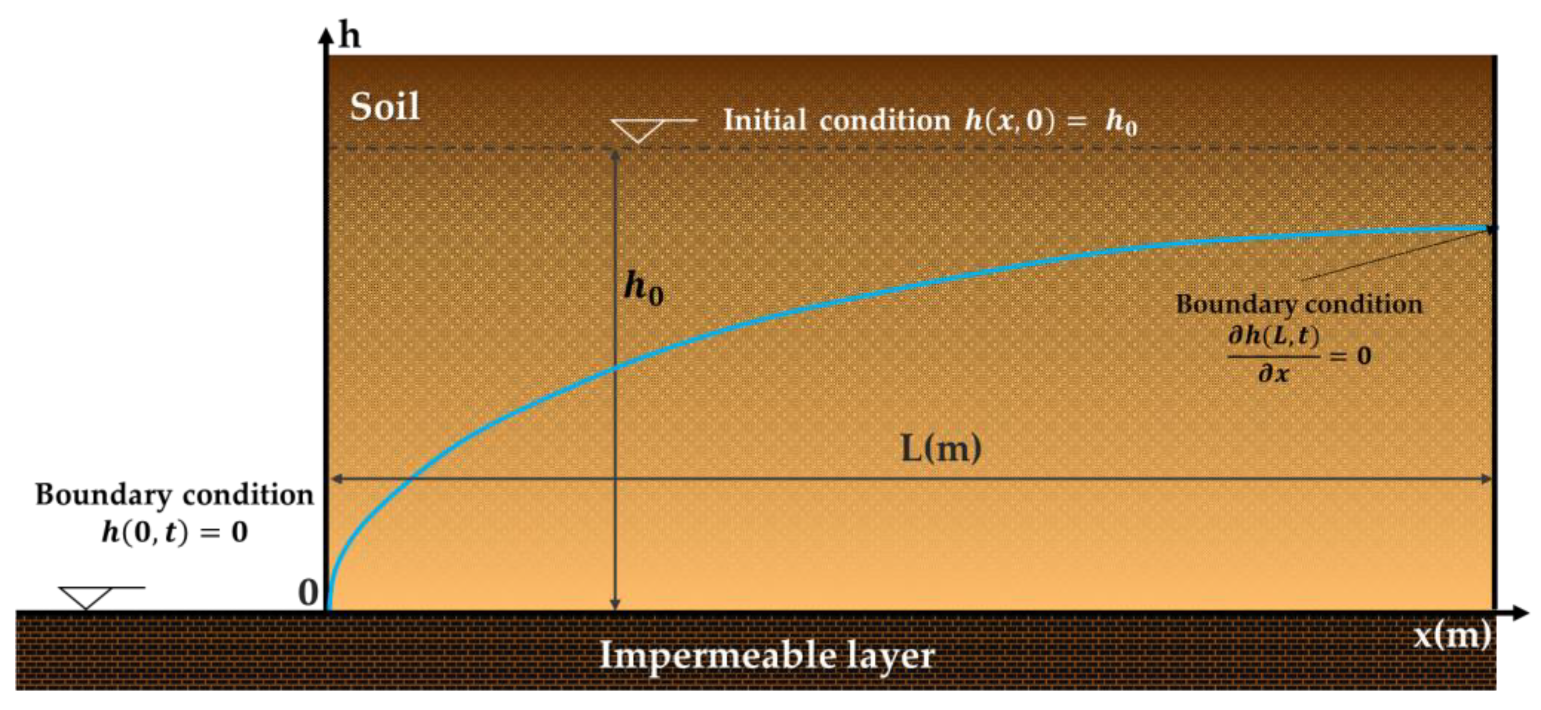
Boussinesq (1904) obtained an exact solution assuming an inverse incomplete beta function as the initial condition for the groundwater table. In addition to the above simplifications, he assumed that (a) the water level in the channel at x = 0 was equal to zero and (b) that the boundary condition at x = L was that the flux q(L, t) = 0, that is in this position there is an impermeable geological formation.

In case of drainage problem with drains overlying an impermeable layer and drain spacing between 2L, due to symmetry in water level, there is the same boundary condition to x = L (q(L, t) = 0), and the Boussinesq solution could be valid. This equation was presented by Boussinesq (1904) in the French journal ‘Journal de Mathématiques Pures et Appliquées [1]. Polubarinova Kochina [2,3,4] published a solution to Boussinesq’s equation using the method of small disturbances. Tolikas et al. (1984) [5] obtained an approximate closed-form solution by applying similarity transformation and polynomial approximation. Lockington (1997) [6] provided a simple approximate analytical solution using a weighted residual method. This method was applied to both the recharging and discharging of an unconfined aquifer due to a sudden change in the head at the origin. Moutsopoulos (2010) [7] applied Adomian’s decomposition method and obtained a simple series solution with a few terms, and performing a benchmark test showed the advantages of his solution. Basha (2013) [8] used the traveling wave method to obtain a nonlinear solution of a simple logarithmic form. The solution is adaptable to any flow situation that is recharged or discharged and allows practical results in hydrology. Additionally, algebraic equations are included for the velocity of the propagation front, wetting front position, and relationship for aquifer parameters. Chor et al. (2013) [9] provided a series solution for the nonlinear Boussinesq equation in terms of the Boltzmann transform in a semi-infinite domain. More recently, Hayek (2019) [10] provided an approximate solution by introducing an empirical function with four parameters. The parameters were obtained using a numerical fitting procedure with the add-in Solver tool in Microsoft Excel. Furthermore, analytical approaches are based mainly on Caputo fractional derivatives explored by authors to provide solutions to nonlinear partial differential equations. Specifically, Khan et al. (2019) [11] proposed a hybrid methodology of Shehu transformation along with the Adomian decomposition method, while Shah et al. (2019) [12] and Rashid et al. (2021) [13] provided solutions to a system of nonlinear fractional Kortweg-de Vries partial differential equations based on Caputo operator, Shehu decomposition method, and the Shehu iterative transform method. Iqbal et al. (2022) [14] used a novel iterative transformation technique and homotopy perturbation transformation technique to calculate. The fractional-order gas dynamics equation. Tzimopoulos et al. (2021) [15] used a transformed method of Wiedeburg (1980) [16] to solve the one-dimensional Boussinesq equation for both the recharging and discharging of a homogeneous unconfined aquifer. Several other authors provide useful insight into the solution and are valuable tools for testing the accuracy of numerical methods [17,18,19,20,21,22,23].

Due to the difficulty of finding exact analytical solutions to the physical problem, many numerical solutions to the problem of the water response to recharge or discharge of an aquifer have been developed in the past. Remson et al. (1971) [24] give detailed information about the existing numerical methods for solving problems in subsurface hydrology. Tzimopoulos and Terzides (1975) [25] investigated the case of water movement through soils drained by parallel ditches. Numerical solutions are presented based on implicit computational schemes of the Crank–Nicolson, Laasonen, and Douglas types. Experimental data obtained by a Hele-Shaw model in the laboratory are in very good agreement with the values computed numerically by these implicit schemes. Chávez et al. (2011) [26] considered a problem of agricultural drainage described by the Boussinesq equation. They implemented an implicit numerical scheme in which interpolation parameters were used, that is γ and ω, for space and time, respectively. Two discretization schemes of the time derivative were found: the mixed scheme and the head scheme. Both schemes were validated with one analytical solution. Bansal (2012) [27] and Bansal (2016) [28] investigated the case of groundwater fluctuations in sloping aquifers induced by replenishment and seepage from a stream. For this case, the Boussinesq equation has been discretized using the Mac Cormack scheme. This scheme is a predictor–corrector scheme in which the predicted value of the head is obtained by replacing the spatial and temporal derivatives with forward differences. The corrector scheme is obtained by replacing the spatial derivative with a backward difference and the time derivative with a forward difference. Borana et al. (2013) [29] employed a Crank–Nicolson finite-difference scheme to solve the Boussinesq equation for the case of infiltration phenomenon in a porous medium. They concluded that the Crank–Nicolson scheme is consistent with the physical phenomenon and stable without any restrictions on the stability ratio. Bansal (2017) [30] investigated the case of the interaction of surface and groundwater in a stream-aquifer system. He derived a new analytical solution and employed the Du Fort and Frankel scheme for the comparison. The proposed scheme is an explicit finite-difference numerical scheme, proceeding in three time levels. Nguyen (2018) [31] investigated the case of stratified heterogeneous porous media. The model is a system of two equations: one for the water level in fissured porous blocks and one for the water level in system cracks. The discretized schemes are explicit in both cases. More recently, Samarinas et al. (2018, 2021) [32,33] developed the Crank–Nicolson scheme in a fuzzy environment and solved the linearized fuzzy Boussinesq equation while later proposing an efficient method to solve the fuzzy tridiagonal system of equations that appeared in the numerical scheme [34].

An alternative numerical method based on the weak variational formulation of boundary and initial value problems is the Finite Elements Method (FEM). It is a popular method for numerically solving partial differential equations arising in engineering and mathematical modeling, including traditional fields of structural analysis, heat transfer, fluid flow, mass transport, and electromagnetic potential. The pioneers of this method are considered Courant (1943) [35], Argyris (1954) [36], and Turner et al. (1956) [37]. According to Oden (1990) [38], “no other family of approximation methods has had a greater impact on the theory and practice of numerical methods during the twentieth century”. Many numerical solutions based on the FEM method and concerning hydraulic problems have been presented. Tzimopoulos and Terzides (1976) [39] studied a physical problem of a free surface flow toward a ditch or a river. The solution to Boussinesq’s equation was made by the application of the finite-element method. Galerkin’s method [40] was used, leading to a system of nonlinear equations. Numerical results were compared with the exact solution of Boussinesq and with other finite-difference approximations. Frangakis and Tzimopoulos (1979) [41] investigated a numerical model based on Boussinesq’s equation describing the unsteady groundwater flow on impervious sloping bedrock. The numerical model uses the finite-element technique with Galerkin’s method. The stability and accuracy of the method have been proved by the comparison of numerical results with the Crank–Nicolson scheme. Tzimopoulos and Tolikas (1980) [42] investigated the problem of artificial groundwater recharge in the case of an unconfined aquifer, described by the Boussinesq equation. The problem was solved by analytical and numerical methods. The finite-element method was used with square elements. Tber and Talibi (2007) [43] presented a numerical method of FEM to automatically identify hydraulic conductivity in the seawater intrusion problem when a sharp interface approach is used. Mohammadnejad and Khoei (2013) [44] presented a fully coupled numerical model developed for the modeling of hydraulic fracture propagation in porous media, using the extended finite element method in conjunction with the cohesive crack model. Yang et al. (2019) [45] proposed a novel computational methodology to simulate the nonlinear hydro-mechanical process in saturated porous media containing crossing fractures. The nonlinear hydro-mechanical coupled equations are obtained using the Extended Finite Element Method (XFEM) discretization and solved using the Newton-Raphson method. Aslan and Temel (2022) [46] described the 2D steady-state seepage analysis of the dam body and its base is investigated using the Finite element method (FEM) based on Galerkin’s method [40] and Ritz’s (1908) [47] approach. The body and foundation soil are considered homogeneous isotropic and anisotropic materials, and the effects of horizontal drainage length and the cutoff wall on seepage are investigated.

Since the aforementioned problem concerns differential equations, which present particular problems regarding fuzzy logic, a significant number of research studies were carried out in that field, especially regarding the fuzzy differentiation of functions. Initially, fuzzy differentiable functions were studied by Puri and Ralescu (1983) [48], who generalized and extended Hukuhara’s fundamental study [49] (H-derivative) of a set of values appearing in fuzzy sets. Kaleva (1987) [50] and Seikkala (1987) [51] developed a theory on fuzzy differential equations. In the last years, several studies have been carried out in the theoretical and applied research field on fuzzy differential equations with an H-derivative [50,52,53,54]. Nevertheless, in many cases, this method has presented certain drawbacks since it has led to solutions with increasing support, along with increasing time [55]. This proves that, in some cases, this solution is not a representative generalization of the classic case. To overcome this drawback, the generalized derivative gH (gH-derivative) was introduced [56,57,58]. The gH-derivative will henceforth be used for a more extensive degree of fuzzy functions than the Hukuhara derivative.

In general, fuzzy methodology has already been recognized as an innovative approach to handling problem uncertainties with several works in different scientific fields [59,60,61,62,63] but to our knowledge, a limited number of studies have been published recently concerning fuzzy FEM models and are mainly in structural mechanics [31,64,65,66,67].

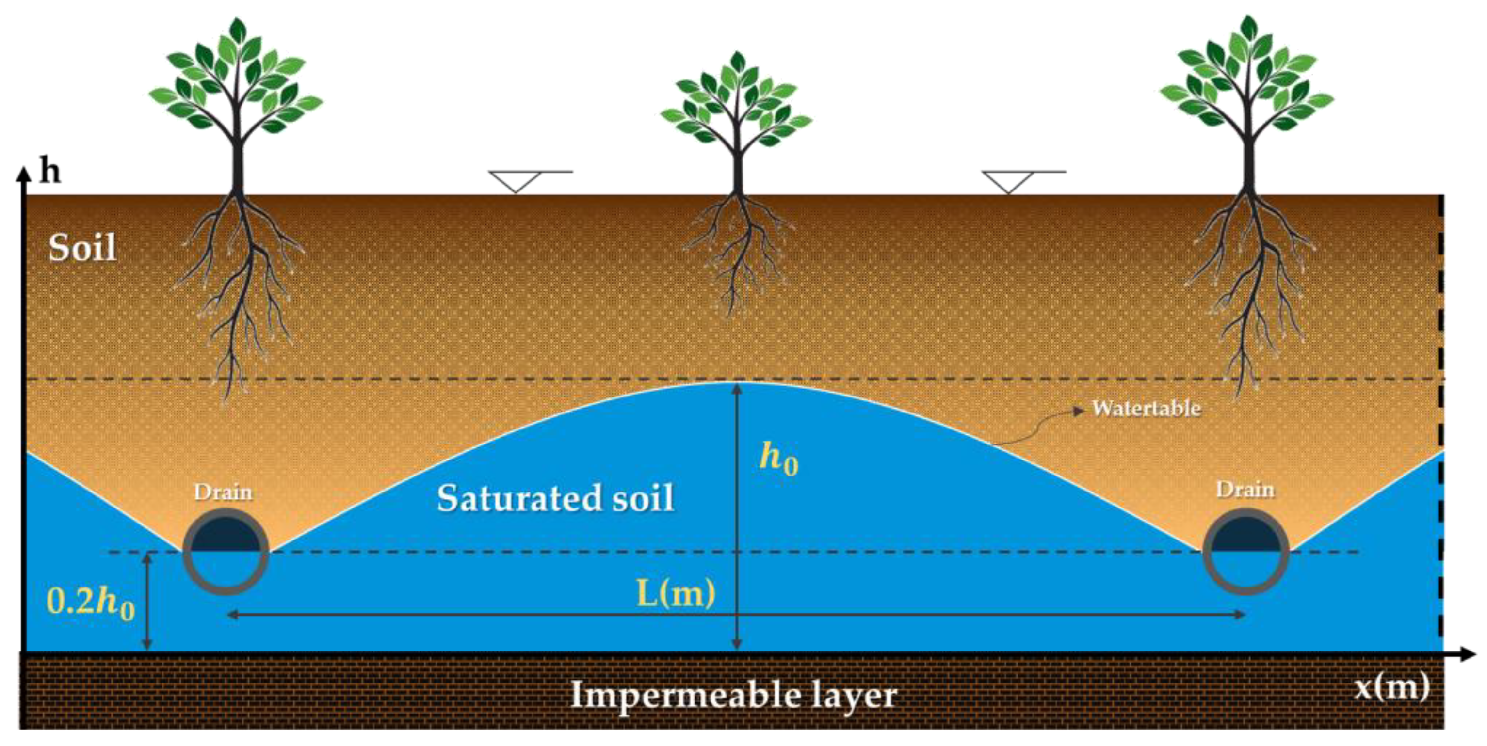
In the present article, two crucial hydraulic properties (Conductivity K and Porosity S) on the Boussinesq equation are considered fuzzy, and the overall problem is encountered with a new approximate fuzzy FEM numerical solution, leading to a system of crisp boundary value problems. In the current work, two different physical problems of fuzzy, unsteady nonlinear flow are examined: (a) the case of a drainage problem, with drains overlying an impermeable layer without precipitation, and (b) the case of a semi-infinite unconfined aquifer bordering a geological formation and overlying an impermeable layer. 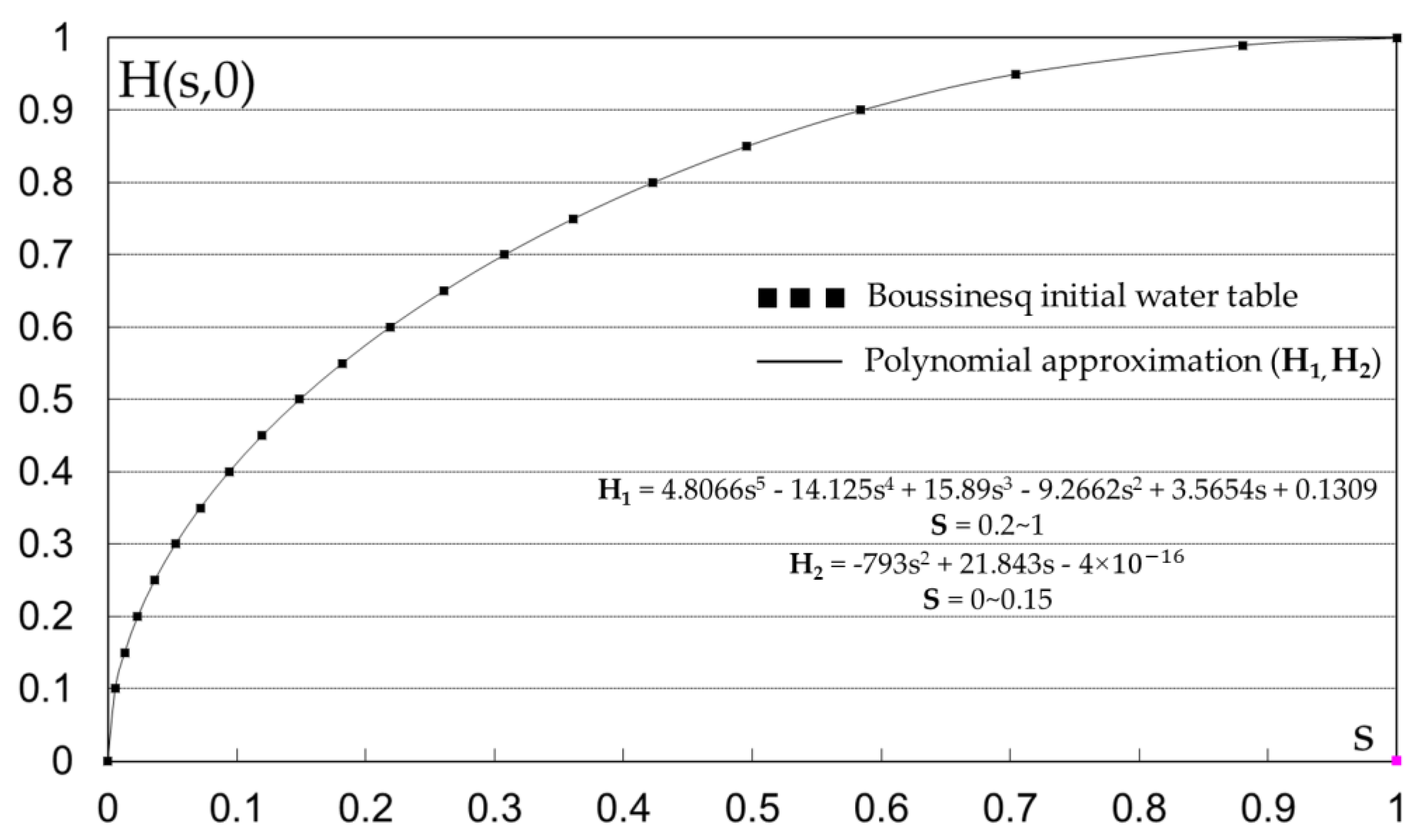In the first case, the initial water table is equal to h₀. The water table is falling, and outflow volume is flowing to the two drains. 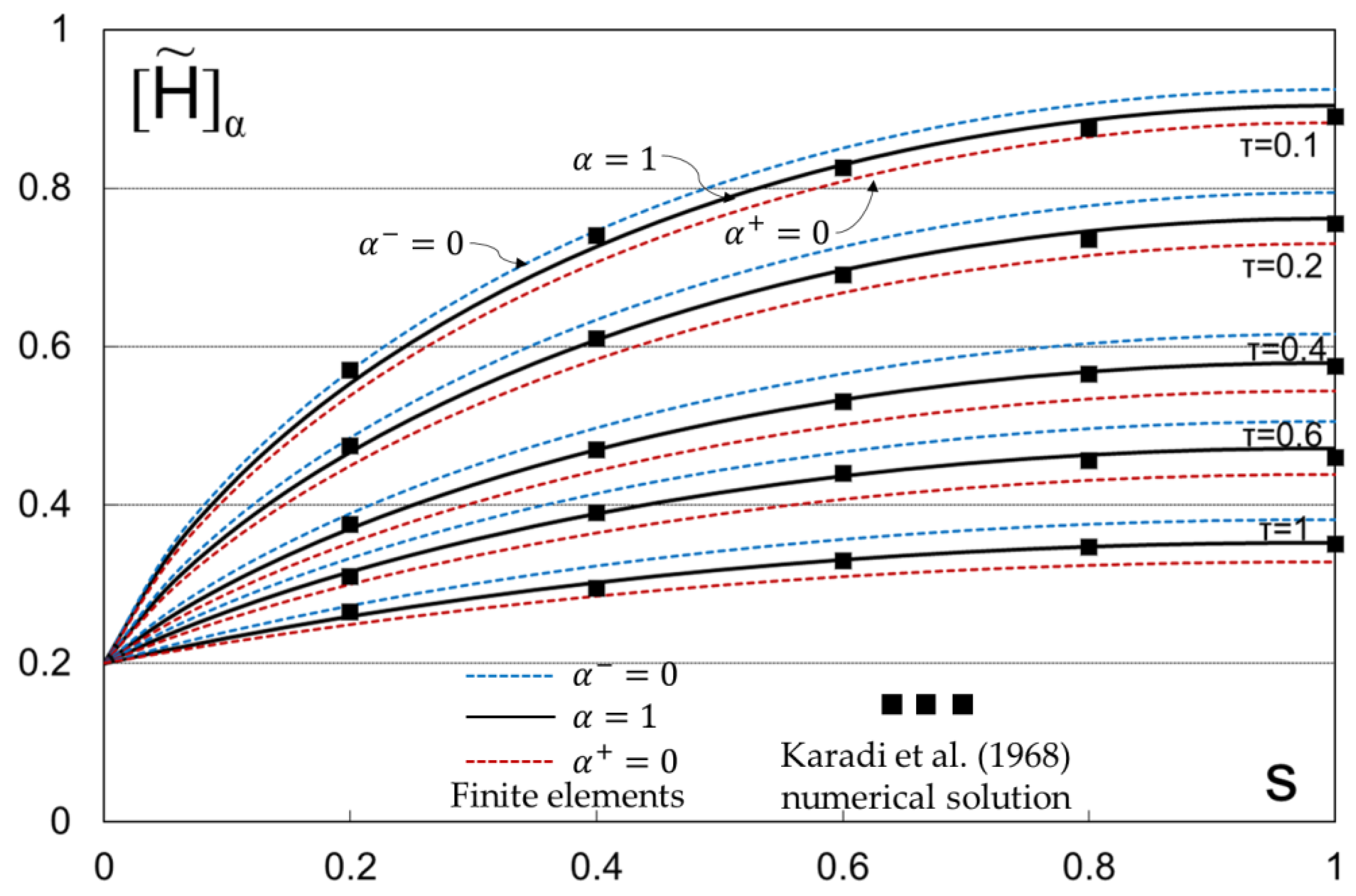In the second case (considering the Boussinesq solution [1]), the initial groundwater table had the form of an inverse incomplete beta function, which in the current study has been approximated by polynomial approximation presented in very close agreement with the initial form. The proposed FEM method has proved to be in agreement with other numerical method by Karadi et al. 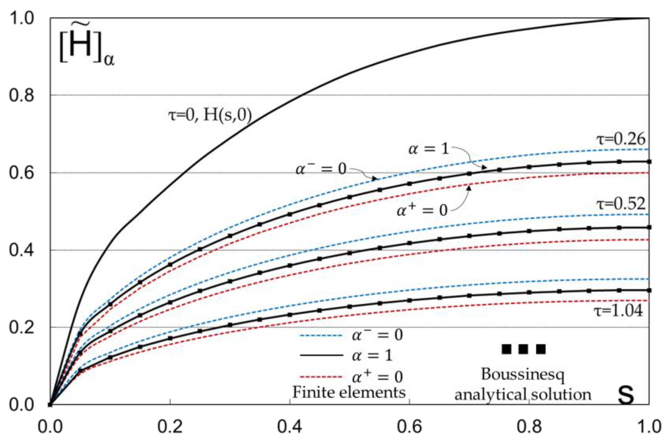1968 [68] and in close agreement with the Boussinesq analytical method [1]. In addition, this work presents a specific novelty related to fuzzy FEM, as a limited number of studies have been published recently concerning only structural mechanics. Additionally, in the current work, the possibility theory and the fuzzy theory combined led to fuzzy estimators for the hydraulic parameters (water levels and outflow volumes). Therefore, engineers and designers can have a complete picture of the influence of these parameters, and by knowing the confidence intervals with a certain strong probability and a small risk can help them make the right decisions for water resource projects.

2. Materials and Methods

2.1. Crisp Model

For the convenience of the reader throughout this work, the following sketch (Figure 1) is provided, in which valuable definitions regarding the physical problem under examination are provided.

The free surface of the groundwater flow to the drains is described by the Boussinesq equation:

$$\frac{\partial h}{\partial t}=\frac{K}{S}\frac{\partial }{\partial x}\left(h\frac{\partial h}{\partial x}\right)$$

(1)

with the following initial and boundary flow conditions:

$$\begin{gathered} t=0,h\left(x,0\right)=h_0, \\ t>0,h\left(0,t\right)=0,\frac{\partial h\left(L,t\right)}{\partial x}=0. \end{gathered}$$

(2)

Now, nondimensional variables are introduced:

$$H=\frac{h}{h_0},s=\frac{x}{L},\tau =\frac{K{h}_{0}t}{2S{L}^2},$$

(3)

and Equation (1) is then transformed into the following expression:

$$\frac{\partial H}{\partial \tau }=\frac{\partial }{\partial s}\left(2H\frac{\partial H}{\partial s}\right),$$

(4)

with the following new initial and boundary flow conditions:

$$\begin{gathered} \tau =0,H\left(s,0\right)=1, \\ \tau >0,H\left(0,\tau \right)=0,\frac{\partial \left(H\left(1,\tau \right)\right)}{\partial s}=0. \end{gathered}$$

(5)

Numerical Method

For the solution of Equation (4), the FEM has been used. The domain of integration (s, τ) is divided into rectangular elements with dimensions Δs and Δτ/2. The global nodal points are numbered with bold numbers 1, 2, ..., and G, while the local ones inside each element are numbered with large numbers N = (1), (2), (3), and (4) enclosed in parentheses. Each element (e) is also numbered with small letters enclosed in parentheses (e₁), (e₂), …., (e_n) (Figure 2b). Equation (4) is not linear, so the more suitable numerical method for the construction of a model with finite elements is Galerkin’s method [69].

By using this method, Equation (4) is written:

$$L\left(\stackrel{-}{H}\right)=\frac{\partial \stackrel{-}{H}}{\partial \tau }-\frac{\partial }{\partial s}\left(2\stackrel{-}{H}\frac{\partial \stackrel{-}{H}}{\partial s}\right)=r_0,$$

(6)

where $r_0=\mathrm{a}\mathrm{smal}\mathrm{quantity},\mathrm{and}\stackrel{-}{H}=\mathrm{an}\mathrm{approximating}\mathrm{function}\mathrm{to}\mathrm{H}.$

In Galerkin’s method, the global basis function ${\Phi }_{\mathsf{\Delta }}(\overrightarrow{X})$ (Figure 2a) is orthogonal with respect to operator $L(\stackrel{-}{H})$, that is:

$${{\displaystyle \int }}_{R}L(\stackrel{-}{H}){\Phi }_{\mathsf{\Delta }}(\overrightarrow{X})dR=0,\overrightarrow{X}=\left(s,\tau \right),\mathsf{\Delta }=1,2,....,G.$$

(7)

Note: from now on, the dash over H will be omitted for practical reasons.

By using Green’s theorem, Equation (7) gives the nonlinear algebraic equation as follows:

$$\begin{gathered} -\lambda [{\mathsf{\Delta }}_{i,j+\frac{1}{2}}^2\left(H^2\right)+\frac{1}{6}{\mathsf{\Delta }}_{i,j}^2\left(H^2\right)+\frac{1}{6}{\mathsf{\Delta }}_{i,j+1}^2\left(H^2\right)+\frac{1}{3}\{H_{i-1,j+\frac{1}{2}}\left(H_{i-1,j}+H_{i-1,j+1}\right)-2H_{i,j+\frac{1}{2}}\left(H_{i,j}+H_{i,j+1}\right)+ \\ {H}_{i+1,j+\frac{1}{2}}\left(H_{i+1,j}+H_{i+1,j+1}\right)\}]+\frac{1}{6}\left\{\left(H_{i-1,j+1}+4H_{i,j+1}+H_{i+1,j+1}\right)-\left(H_{i-1,j}+4H_{i,j}+H_{i+1,j}\right)\right\}=0, \\ i=1,2,....,n,j=1,2,\dots \dots k, \end{gathered}$$

(8)

where λ = Δτ/Δs² and the operator ${\mathsf{\Delta }}_{i,j}^2\left(H^2\right)=H_{i+1,j}^2-2H_{i,j}^2+H_{i-1,j}^2$. The nonlinear terms are linearized by taking

$$H_{i,j+1}^2=H_{i,j}^2+\frac{\partial \left(H^2\right)}{\partial H}\left|i,j(\right.H_{i,j+1}-H_{i,j}),$$

(9)

and the functions at the point (i, j + 1/2) are approximated by

$${(H^2)}_{i,j+1/2}=\frac{1}{2}({(H^2)}_{i,j}+\left(H^2{)}_{i,j+1}\right).$$

(10)

Under the above simplifications, the linearized equation becomes:

$$A_i{X}_{i-1,j+1}+B_i{X}_{i,j+1}+C_i{X}_{i+1,j+1}=D_i$$

(11)

with

$$\begin{gathered} A_i=-\lambda H_{i-1,j}+\frac{1}{6}, \\ {B}_i=2\lambda H_{i,j}+\frac{2}{3}, \\ {C}_i=-\lambda H_{i+1,j}+\frac{1}{6}, \\ D_i=\frac{1}{6}\left(H_{i+1,j}+4H_{i,j}+H_{i-1,j}\right) \\ {X}_{i-1,j+1}\equiv H_{i-1,j+1},X_{i,j+1}\equiv H_{i,j+1},X_{i+1,j+1}\equiv H_{i+1,j+1}. \end{gathered}$$

The solution of Equation (11) is obtained via the Thomas algorithm [70] for tridiagonal systems. It is also crucial to mention that this algorithm is a special adaptation of the Gauss elimination method, and it is very efficient if the following relation is applied in a computer [25]:

$$\begin{gathered} A_i>0, B_i>0, C_i>0, D_i>0 \\ \lambda >\frac{1}{H_{i-1,j}-2H_{i,j}+H_{i+1,j}}. \end{gathered}$$

In the current work, the values of $\mathsf{\Delta }t=0.006d \mathrm{and} \mathsf{\Delta }{x}^2=1.5m$ used provide numerical stability for all cases.

2.2. Fyzzy Framework and Definitions

For readers unfamiliar with the fuzzy theory, we describe definitions concerning some preliminaries in fuzzy theory and definitions of the differentiability.

Definition 1. 

A fuzzy set $\tilde{U}$ on a universe set Χ is mapping  $\tilde{U}:X\to \left[0,1\right]$, assigning to each element  $x\in X$ a degree of membership  $0\le \tilde{U}\left(x\right)\le 1$. The membership function  $\tilde{U}\left(x\right)$ is also defined as  ${\mu }_{\tilde{U}}\left(x\right)$ with the properties:

(i) ${\mu }_{\tilde{U}}$ is upper semicontinuous;

(ii)  ${\mu }_{\tilde{U}}\left(x\right)$ = 0, is outside of some interval [c, d];

(iii) there are real numbers  $c\le a\le b\le d$, such that  ${\mu }_{\tilde{U}}$ is monotonic nondecreasing on [c,a], and monotonic nonincreasing on [b, d] and  ${\mu }_{\tilde{U}}\left(x\right)$ = 1 for each  $x\in \left[a,b\right]$;

(iv)  $\tilde{U}$ is a convex fuzzy set (i.e., ${\mu }_{\tilde{U}}\left(\lambda x+\left(1-\lambda \right)x\right)\ge \min \{{\mu }_{\tilde{U}}\left(\lambda x\right),{\mu }_{\tilde{U}}\left(\left(1-\lambda \right)x\right)\}$.

Definition 2. 

Let X be a Banach space and  $\tilde{U}$ be a fuzzy set on X. We define the α-cuts of  $\tilde{U}$ as  ${[\tilde{U}]}^{\alpha }=\left\{x\in R\left|\tilde{U}\left(x\right)\ge \alpha \right.\right\}, \alpha \in \left(0,1\right]$ are defined, and forα=0, the closure is

$${[\tilde{U}]}^0=\stackrel{--------------}{\left\{x\in R\left|\tilde{U}\left(x\right)>0\right.\right\}}$$

Definition 3. 

Let Ҡ(X) be the family of all nonempty compact convex subsets of a Banach space. A fuzzy set  $\tilde{U}$ on X is called compact if  ${[\tilde{U}]}_{\alpha }\in$ Ҡ(X),  $\forall \alpha \in \left[0,1\right].$ The space of all compact and convex fuzzy sets on X is denoted as Ƒ (X).

Definition 4. 

Let  $\left[\tilde{U}\right]\in$ Ƒ (R). The α-cuts of  $\tilde{U}$ are  ${\left[\tilde{U}\right]}_{\alpha }=[U_{\alpha }^{-},U_{\alpha }^{+}]$ . According to the representation theorem of [71] and the theorem of [72], the membership function and the α-cut form of a fuzzy number $\tilde{U}$ are equivalent, and, in particular, the α-cuts  ${\left[\tilde{U}\right]}_{\alpha }=[U_{\alpha }^{-},U_{\alpha }^{+}]$ uniquely represent  $\tilde{U}$, provided that the two functions are monotonic ($U_{\alpha }^{-}$ monotonic nondecreasing,  $U_{\alpha }^{+}$ monotonic nonincreasing) and  $U_{\alpha =1}^{-}\le U_{\alpha =1}^{+}$ for a = 1.

Definition 5. 

gH-differentiability [73]. Let $\tilde{U}:\left[a,b\right]\to$ R_Ƒ be such that  $\left[\tilde{U}\left(x\right){]}_{\alpha }]=\right[U_{\alpha }^{-}\left(x\right),U_{\alpha }^{+}\left(x\right)]$. Suppose that the functions  $U_{\alpha }^{-}\left(x\right)$ and  $U_{\alpha }^{+}\left(x\right)$ are real-valued functions, differentiable w.r.t. x, and uniformly w.r.t.  $\alpha \in \left[0,1\right]$. Then, the function  $\tilde{U}$ is gH-differentiable at a fixed  $x\in \left[a,b\right]$ if, and only if, one of the following two cases holds:

• ${\left(U_{\alpha }^{-}\right)}^{\prime }\left(x\right)$ is increasing,  ${\left(U_{\alpha }^{+}\right)}^{\prime }\left(x\right)$ is decreasing as functions of α, and
• $\left[{\left(U_{\alpha =1}^{-}\right)}^{\prime }\left(x\right)\le {\left(U_{\alpha =1}^{+}\right)}^{\prime }\left(x\right)\right]$, or
• ${\left(U_{\alpha }^{+}\right)}^{\prime }\left(x\right)$ is increasing,${\left(U_{\alpha }^{-}\right)}^{\prime }\left(x\right)$ is decreasing as functions of α, and  $\left[{\left(U_{\alpha =1}^{+}\right)}^{\prime }\left(x\right)\le {\left(H_{\alpha =1}^{-}\right)}^{\prime }\left(x\right)\right]$

Note:  ${\left(U_{\alpha }^{-}\right)}^{\prime }\left(x\right)=\frac{d{U}_{\alpha }^{-}\left(x\right)}{dx},{\left(U_{\alpha }^{+}\right)}^{\prime }\left(x\right)=\frac{d{U}_{\alpha }^{+}\left(x\right)}{dx}$. In both of the above cases, the  ${\tilde{U}}_{\alpha }^{\prime }\left(x\right)$ derivative is a fuzzy number.

Definition 6. 

gH-differentiable at x₀. Let  $\tilde{U}:\left[a,b\right]\to$ R_F and  $x_0\in \left[a,b\right]$ with  $U_{\alpha }^{-}\left(x\right)$ and  $U_{\alpha }^{+}\left(x\right),$ and both be differentiable at x₀. We say that [73]:

• $\tilde{U}$ is (i)-gH-differentiable at x₀ if:

  $$(\mathrm{i})\left[{\tilde{U}}_{gH}^{\prime }\left(x_0\right){]}_{\alpha }=\right[{(U_{\alpha }^{-})}^{\prime }\left(x_0\right),U_{\alpha }^{+}{)}^{\prime }\left(x_0\right)],\forall \alpha \in 0,1$$
• $\tilde{H}$ is (ii)-gH-differentiable at x₀ if:

  $$(\mathrm{ii})\left[{\tilde{U}}_{gH}^{\prime }\left(x_0\right){]}_{\alpha }=\right[{(U_{\alpha }^{+})}^{\prime }\left(x_0\right),\left(U_{\alpha }^{-}{)}^{\prime }\left(x_0\right)\left],\forall \alpha \in \right[0,1\right]$$

Definition 7. 

g-differentiability. Let  $\tilde{U}:\left[a,b\right]\to$R_F be such that  $\left[\tilde{U}\left(x\right){]}_{\alpha }=\right[U_{\alpha }^{-}\left(x\right),U_{\alpha }^{+}\left(x\right)]$. If  $U_{\alpha }^{-}\left(x\right)$ and  $U_{\alpha }^{+}\left(x\right)$ are differentiable real-valued functions with respect to x, and uniformly for  $\alpha \in \left[0,1\right]$, then  $\tilde{U}\left(x\right)$ is g-differentiable and we have [29]:

$${[{\tilde{U}}_g^{\prime }\left(x\right)]}_{\alpha }=\left[\underset{\beta \ge \alpha }{inf}\min \{{(U_{\alpha }^{-})}^{\prime }\left(x\right),{(U_{\alpha }^{+})}^{\prime }\left(x\right)\},\underset{\beta \ge \alpha }{sup}\max \{{(U_{\alpha }^{-})}^{\prime }\left(x\right),{(U_{\alpha }^{+})}^{\prime }\left(x\right)\}\right]$$

Definition 8. 

The gH-differentiability implies g-differentiability, but the inverse is not true.

Definition 9. 

[gH-p] differentiability. A fuzzy-valued function  $\tilde{U}$ of two variables is a rule that assigns to each ordered pair of real numbers (x, t) in a set D a unique fuzzy number denoted by  $\tilde{U}\left(x,t\right)$. Let  $\tilde{U}\left(x,t\right)$: D→ R_Ƒ, (x₀, t₀)  $\in$ D and  $U_{\alpha }^{-}\left(x,t\right)$,  $U_{\alpha }^{+}\left(x,t\right)$ are real-valued functions and partial differentiable w.r.t. x. We say that [58,74]:

• $\tilde{U}$ is [(i)-p]-differentiable w.r.t. x at (x₀, t₀) if:

  $$\frac{\partial {\tilde{U}}_{\alpha }\left(x_0,t_0\right)}{\partial x_{i.gH}}=\left[\frac{\partial U_{\alpha }^{-}\left(x_0,t_0\right)}{\partial x},\frac{\partial U_{\alpha }^{+}\left(x_0,t_0\right)}{\partial x}\right]$$
• $\tilde{U}$ is [(ii)-p]-differentiable w.r.t. x at (x₀, t₀) if:

  $$\frac{\partial {\tilde{U}}_{\alpha }\left(x_0,t_0\right)}{\partial x_{i.gH}}=\left[\frac{\partial U_{\alpha }^{+}\left(x_0,t_0\right)}{\partial x},\frac{\partial U_{\alpha }^{-}\left(x_0,t_0\right)}{\partial x}\right]$$

Notation. The same is valid for  $\frac{\partial {\tilde{H}}_{\alpha }\left(x_0,t_0\right)}{\partial t}$.

Definition 10. 

Let  $\tilde{U}\left(x,t\right)$: D→R_Ƒ, and  $\frac{\partial {\tilde{U}}_{\alpha }\left(x_0,t_0\right)}{\partial x_{i.gH}}$ be [gH-p]-differentiable at (x₀, t₀)  $\in$ D with respect to x. We say that [58,74]:

• $\frac{\partial U_{\alpha }\left(x_0,t_0\right)}{\partial x_{i.gH}}$ is [(i)-p]-differentiable w.r.t.x if:

  $$\frac{{\partial }^2{\tilde{U}}_{\alpha }\left(x_0,t_0\right)}{\partial {x^2}_{i.gH}}=\left\{\begin{array}{c}\left[\frac{{\partial }^2{U}_{\alpha }^{-}\left(x_0,t_0\right)}{\partial x^2},\frac{{\partial }^2{U}_{\alpha }^{+}\left(x_0,t_0\right)}{\partial x^2}\right]if\tilde{U}\left(x,t\right)is\left[\left(i\right)-p\right]differentiable\\ \left[\frac{{\partial }^2{U}_{\alpha }^{+}\left(x_0,t_0\right)}{\partial x^2},\frac{{\partial }^2{U}_{\alpha }^{-}\left(x_0,t_0\right)}{\partial x^2}\right]if\tilde{U}\left(x,t\right)is\left[\left(ii\right)-p\right]differentiable\end{array}\right.$$
• $\frac{\partial {\tilde{H}}_{\alpha }\left(x_0,t_0\right)}{\partial x_{i.gH}}$ is [(ii)-p]-differentiable w.r.t.x if:

  $$\frac{{\partial }^2{\tilde{U}}_{\alpha }\left(x_0,t_0\right)}{\partial {x^2}_{i.gH}}=\left\{\begin{array}{c}\left[\frac{{\partial }^2{U}_{\alpha }^{+}\left(x_0,t_0\right)}{\partial x^2},\frac{{\partial }^2{U}_{\alpha }^{-}\left(x_0,t_0\right)}{\partial x^2}\right]if\tilde{U}\left(x,t\right)is\left[\left(i\right)-p\right]differentiable\\ \left[\frac{{\partial }^2{U}_{\alpha }^{-}\left(x_0,t_0\right)}{\partial x^2},\frac{{\partial }^2{U}_{\alpha }^{+}\left(x_0,t_0\right)}{\partial x^2}\right]if\tilde{U}\left(x,t\right)is\left[\left(ii\right)-p\right]differentiable\end{array}\right.$$

2.2.1. Possibility Theory

Below, we provide critical definitions regarding the possibility theory that is implemented in the current work.

Definition 11. 

A possibility measure,  $\Pi ,$ on a set,   $X$ (e.g., a set of reels), is characterized by a possibility distribution of  $\pi \to \left[0,1\right]$ and is defined by the following:

$$A\subseteq X,\Pi \left(A\right)=sup(\pi \left(x\right),x\in A).$$

For finite sets, this definition reduces to the following:

$$\forall A\subseteq X,\Pi \left(A\right)=max\left(\pi \left(x\right),x\in A\right).$$

Definition 12. 

A degree of necessity, Ness  $X,$ on a set  $X$ (e.g., a set of reels), is characterized by the non-possibility (one minus possibility) of A complement (A^C).

Definition 13. 

A probability distribution p and a possibility distributionπ are said to be consistent only if  $\pi \left(u\right)\ge p\left(u\right),\forall u$[75,76].

Definition 14. 

Two possibility distributions, π_x and π′_x, are consistent with the probability distribution p_x. The π_x distribution is more specific than π′_x if π_x < π′_x. A possibility distribution of π′_x consistent with the probability distribution p_x is called maximal specificity if it is more specific than the other possibility distribution:

$${\pi }_x:\pi {\prime }_x\left(x\right)<{\pi }_x\left(x\right),\forall x.$$

Definition 15. 

For a number Y with a known and continuous probability distribution function p, the fuzzy number  $\tilde{Y}$, which has a possibility measure  $\Pi \left(\tilde{Y}\right)={\mu }_{\tilde{Y}}$ is the fuzzy estimator of Y and has an α-cut of  ${\Pi }_{\tilde{Y}}\left(\alpha \right)=\tilde{Y}\left(\alpha \right).$ This fuzzy number satisfies the consistency principle and verifies  ${\Pi }_{\tilde{Y}}\left(\alpha \right)=Ness\tilde{Y}\left(\alpha \right)=1-\alpha$, so that the probability of the possibility α-cut is equal to 1 − α. The α-cuts  $\tilde{Y}\left(\alpha \right)$ are the confidence intervals of P, and the confidence level is α.

Definition 16. 

Conjecture [76]. For a function Y = Y (X₁, X₂, ....X_n) with an unknown probability distribution function, a fuzzy number may be constructed ${\tilde{Y}}^{*}=\tilde{Y}\left({\tilde{X}}_1^{*},{\tilde{X}}_2^{*},....,{\tilde{X}}_n^{*}\right),$ and the α-cut is equal to the following: 

$${\tilde{Y}}^{*}\left(\alpha \right)=\tilde{Y}\left({\tilde{X}}_1^{*}\left(\alpha \right),{\tilde{X}}_2^{*}\left(\alpha \right),....,{\tilde{X}}_n^{*}\left(\alpha \right)\right).$$

In this case, the fuzzy number  ${\tilde{Y}}^{*}$ is the fuzzy estimator of Y and verifies the following: 

$$P\left({\tilde{Y}}^{*}\left(\alpha \right)\right)\ge Ness{\tilde{Y}}^{*}\left(\alpha \right)=1-\alpha$$

 so that the probability of the possibility α-cut is greater than 1 − α.

2.2.2. Fuzzy Model

The parameters K and S of Equation (1) are considered fuzzy (Figure 3). Thus, the function h is fuzzy, as is the nondimensional function H.

Equation (4) is written in its fuzzy form as follows:

$$\frac{\partial \tilde{H}}{\partial \tau }=\frac{\partial }{\partial s}\left(2\tilde{H}\frac{\partial \tilde{H}}{\partial s}\right).$$

(12)

With the new boundary

$$\tau >0,\tilde{H}\left(0,\tau \right)=0,\frac{\partial (\tilde{H}\left(1,\tau \right)}{\partial s}=0$$

(13)

and initial conditions:

$$\tau =0, \tilde{H}\left(s,0\right)=\tilde{1}.$$

Solutions to the fuzzy problem (12) and the boundary and initial conditions (13) can be found utilizing the theory of [23,58,73,74], translating the above fuzzy problem to a system of second-order crisp boundary value problems, hereafter called the corresponding system for the fuzzy problem. Therefore, eight crisp BVP systems are possible for the fuzzy problem with the same initial and boundary conditions.

System (1,1):	System (1,2):
$\frac{\partial H^{-}}{\partial \tau }=H^{-}\frac{{\partial }^2{H}^{-}}{\partial {\xi }^2}+{\left(\frac{\partial H^{-}}{\partial \xi }\right)}^2$ $\frac{\partial H^{-}}{\partial \tau }=H^{-}\frac{{\partial }^2{H}^{-}}{\partial {\xi }^2}+{\left(\frac{\partial H^{+}}{\partial \xi }\right)}^2$	$\frac{\partial H^{+}}{\partial \tau }=H^{+}\frac{{\partial }^2{H}^{+}}{\partial {\xi }^2}+{\left(\frac{\partial H^{+}}{\partial \xi }\right)}^2$ $\frac{\partial H^{+}}{\partial \tau }=H^{+}\frac{{\partial }^2{H}^{+}}{\partial {\xi }^2}+{\left(\frac{\partial H^{-}}{\partial \xi }\right)}^2$
System (1,3):	System (1,4):
$\frac{\partial H^{-}}{\partial \tau }=H^{-}\frac{{\partial }^2{H}^{+}}{\partial {\xi }^2}+{\left(\frac{\partial H^{+}}{\partial \xi }\right)}^2$ $\frac{\partial H^{-}}{\partial \tau }=H^{-}\frac{{\partial }^2{H}^{+}}{\partial {\xi }^2}+{\left(\frac{\partial H^{-}}{\partial \xi }\right)}^2$	$\frac{\partial H^{+}}{\partial \tau }=H^{+}\frac{{\partial }^2{H}^{-}}{\partial {\xi }^2}+{\left(\frac{\partial H^{-}}{\partial \xi }\right)}^2$ $\frac{\partial H^{+}}{\partial \tau }=H^{+}\frac{{\partial }^2{H}^{-}}{\partial {\xi }^2}+{\left(\frac{\partial H^{+}}{\partial \xi }\right)}^2$
System (2,1):	System (2,2):
$\frac{\partial H^{+}}{\partial \tau }=H^{-}\frac{{\partial }^2{H}^{+}}{\partial {\xi }^2}+{\left(\frac{\partial H^{+}}{\partial \xi }\right)}^2$ $\frac{\partial H^{+}}{\partial \tau }=H^{-}\frac{{\partial }^2{H}^{+}}{\partial {\xi }^2}+{\left(\frac{\partial H^{-}}{\partial \xi }\right)}^2$	$\frac{\partial H^{-}}{\partial \tau }=H^{+}\frac{{\partial }^2{H}^{-}}{\partial {\xi }^2}+{\left(\frac{\partial H^{-}}{\partial \xi }\right)}^2$ $\frac{\partial H^{-}}{\partial \tau }=H^{+}\frac{{\partial }^2{H}^{-}}{\partial {\xi }^2}+{\left(\frac{\partial H^{+}}{\partial \xi }\right)}^2$
System (2,3):	System (2,4):
$\frac{\partial H^{+}}{\partial \tau }=H^{-}\frac{{\partial }^2{H}^{-}}{\partial {\xi }^2}+{\left(\frac{\partial H^{-}}{\partial \xi }\right)}^2$ $\frac{\partial H^{+}}{\partial \tau }=H^{-}\frac{{\partial }^2{H}^{-}}{\partial {\xi }^2}+{\left(\frac{\partial H^{+}}{\partial \xi }\right)}^2$	$\frac{\partial H^{-}}{\partial \tau }=H^{+}\frac{{\partial }^2{H}^{+}}{\partial {\xi }^2}+{\left(\frac{\partial H^{+}}{\partial \xi }\right)}^2$ $\frac{\partial H^{-}}{\partial \tau }=H^{+}\frac{{\partial }^2{H}^{+}}{\partial {\xi }^2}+{\left(\frac{\partial H^{-}}{\partial \xi }\right)}^2$

Note: We will hereby restrict ourselves to the solution of the first system (1,1), which is described in detail below. We apply this case since it provides a physical solution to the problem of aquifer recharging from the lake.

According to definition (4), the α-cuts $\left[H^{-\alpha },H^{+\alpha }\right]$ uniquely represent the fuzzy function $\tilde{H}$, and the following fuzzy expression is valid and refers to α-cuts:

$$L\left({\tilde{H}}^{\alpha }\right)=\left[L\left(H^{-\alpha }\right),L\left(H^{+\alpha }\right)\right]$$

(14)

Solution of system (1,1)

System (1,1) could be defined as:

$$\begin{gathered} {[\frac{\partial \tilde{H}}{\partial \tau }-\tilde{H}\frac{{\partial }^2\tilde{H}}{\partial s^2}+{(\frac{\partial \tilde{H}}{\partial s})}^2=0]}_{\alpha } \\ =\left[\frac{\partial H^{-}}{\partial \tau }-H^{-}\frac{{\partial }^2{H}^{-}}{\partial s^2}+{(\frac{\partial H^{-}}{\partial s})}^2=0, \frac{\partial H^{+}}{\partial \tau }-H^{+}\frac{{\partial }^2{H}^{+}}{\partial s^2}+{(\frac{\partial H^{+}}{\partial s})}^2=0\right],\alpha \in \left[0,1\right], \end{gathered}$$

where for convenience, the following is defined:

$$H^{-}\equiv H^{{\alpha }_{left}},H^{+}\cong H^{a_{right}}.$$

For the left side, the boundary conditions and initial conditions are as follows:

$$\begin{gathered} \tau >0,H^{-}\left(0,\tau \right)=0,\frac{\partial \left(H^{-}\left(1,\tau \right)\right)}{\partial s}=0 \\ \tau =0,H^{-}\left(s,0\right)=1^{-} \end{gathered}$$

while for the right side, the boundary and initial conditions are defined as:

$$\begin{gathered} \tau >0,H^{+}\left(0,\tau \right)=0,\frac{\partial \left(H^{+}\left(1,\tau \right)\right)}{\partial s}=0, \\ \tau =0,H+\left(s,0\right)=1^{+} \end{gathered}$$

2.2.3. Fuzzy Finite Elements Solution

• From Equation (3), we have:

$$\tau =\frac{K{h}_{0}t}{2S{L}^2},\mathrm{or}{\tau }_{{\alpha }_i}={(\frac{K}{S})}_{{\alpha }_i}\frac{h_0}{2L^2}{t}_{{\alpha }_i}$$

(15)

where α_i means the α-cut in line i; for simplification, we put the ratio ${(\frac{K}{S})}_{{\alpha }_i}={\nu }_{{\alpha }_i,}$and the above relation becomes:

$${\tau }_{{\alpha }_i}={\nu }_{{\alpha }_i}\frac{h_0}{2L^2}{t}_{{\alpha }_i}$$

and for two different α-cuts α_i, α_j we take:

$$\frac{{\tau }_{{\alpha }_i}}{{\tau }_{{\alpha }_j}}=\frac{{\nu }_{{\alpha }_i}}{{\nu }_{{\alpha }_j}}\frac{t_{{\alpha }_i}}{t_{{\alpha }_j}}\to {\tau }_{{\alpha }_i}={\tau }_{{\alpha }_j}\frac{{\nu }_{{\alpha }_i}}{{\nu }_{{\alpha }_j}}\frac{t_{{\alpha }_i}}{t_{{\alpha }_j}},$$

(16)

and for the same real-time $t_{{\alpha }_i}=t_{{\alpha }_j}$, we have:

$${\tau }_{{\alpha }_i}={\tau }_{{\alpha }_j}\frac{{\nu }_{{\alpha }_i}}{{\nu }_{{\alpha }_j}}.$$

(17)

Therefore, for the solution of Case a, as well as for Case b, solving the crisp nondimensional system (8) and the linearized Equation (11) is sufficient in order to have the solution for the two cases. For every real-time $t_{{\alpha }_i}=t_{{\alpha }_j}$, the nondimensional time ${\tau }_{{\alpha }_i}$ of every α-cut is given by Equation (17). The α-cut α₁ = 0.05 is taken as a basis for Equation (17), and this equation becomes:

$${\tau }_{{\alpha }_i}={\nu }_{{\alpha }_i}\left(\frac{{\tau }_{{\alpha }_1=0.05}}{{\nu }_{{\alpha }_1=0.05}}\right).$$

(18)

2.

Another solution for Case a is putting it in the dimensional form:

$$\frac{\partial h^{-}}{\partial t}=\left(\frac{K}{S}\right)\frac{\partial }{\partial x}\left(h^{-}\frac{\partial h^{-}}{\partial x}\right)$$

in which the value of the ratio (K/S) equals ${\nu }_{{\alpha }_i},\left(i=1,2,\dots ,6\right)$, and this system is solved for every ${\nu }_{{\alpha }_i},\left(i=1,2,\dots ,6\right)$, applying the Equations (8) and (11), transformed in dimensional form. Initial and boundary conditions should also be transformed into dimensional forms. The same is applied to Case b.

Methods 1 and 2 are equivalent and give exactly the same values.

2.2.4. Outflow Volumes

The outflow volume per with for dimensional variables is equal to:

$$\mathrm{\Omega }\left(t_i\right)={{\displaystyle \int }}_0^{L}Sh(x,t_i)dx \left(m^3/m\right),$$

or in nondimensional variables

$$V\left({\tau }_i\right)=\frac{\mathrm{\Omega }\left(t_i\right)}{S{h}_{0}L}={{\displaystyle \int }}_0^{1}H(s,{\tau }_i)ds.$$

In the case of fuzzy numbers, we have:

$$\left[V\left({\tau }_i\right){]}_{{\alpha }_i}=\right[{{\displaystyle \int }}_0^{1}H(s,{\tau }_i)ds{]}_{{\alpha }_i}.$$

It is now easy to find fuzzy estimators of outflow volume for each time, τ_i.

2.3. A Proposed Method to Solve the Crisp and Fuzzy Models

For the convenience of the reader, the following step-by-step solving process is presented in explanatory form.

The Step-by-Step Solving Process
Step 1:	The interval [s0, sN] is divided into N equal parts: $\mathsf{\Delta }s=\frac{\left(s_N-s_0\right)}{N},s_r=s_0+\left(r-1\right)\mathsf{\Delta }s,r=1,2,....,N+1,s_0=0,s_N=1$
Step 2:	τ = τ + Δτ, $\lambda =\frac{\mathsf{\Delta }\tau }{\mathsf{\Delta }{s}^2}$
Step 3:	Initial valuesH(sr,0) sr, r = 1, 2, … N + 1
Step 4:	Boundary values H(0,τ) = H0, $\frac{dH\left(s_{N+1},\tau \right)}{ds}=0\to \frac{H\left(s_{N+2},\tau \right)-H\left(s_N,\tau \right)}{2\mathsf{\Delta }s}=0\to H\left(s_{N+2},\tau \right)=H\left(s_N,\tau \right)$
Step 5:	$\mathrm{Find}\mathrm{coefficients}\overline{A_i,B_i,C_i,D_i}$
Step 6:	Solve the tridiagonal system [34,70]
Step 7:	Put HNEW into HINITIAL
Step 8:	Compute outflow volume V(HNEW)
Step 9:	Print τ, V(τ), HΝΕW values
Step 10:	If $\tau \le {\tau }_{\max }$ go to 2
	end

3. Results—Application

In order to test the efficiency of the present study with other methods, two different cases are used:

• The Karadi et al. (1968) [68] case, and
• The Boussinesq (1904) [1] analytical solution case.

In both cases, the same soil sample was used with the following parameters: A hydraulic conductivity K = 2.121 cm/h and an effective porosity S = 20%. The two parameters follow a normal distribution with $\stackrel{-}{K}=2.121 \mathrm{cm}/\mathrm{h}$ and a standard deviation $\sigma =0.55329\mathrm{cm}/\mathrm{h},$ and S with $\stackrel{-}{S}=0.2$ and standard deviation $\sigma =0.0363$. Figure 3 presents the fuzzy estimators of K, S, and the ratio K/S for different α-cuts (α_i with i = 1, 2, …, and 6), while Figure 4 presents the initial and boundary conditions of the physical problem.

3.1. The Case by Karadi [68]

Karadi et al. (1968) [68] considered the problem of unsteady seepage flow (Figure 4) under the assumption that the porous medium is homogeneous and isotropic. Experimental data were obtained from a sand model with the following boundary and initial conditions:

$$h\left(0,t\right)=0.2h_0,h\left(L,t\right)=0.2h_0$$

$$h\left(x,0\right)=h_0.$$

This problem corresponds to a drainage problem with an initial water table equal to h₀. For $t>0$ the water table is falling, and outflow volume is flowing to the two drains. Karadi et al. (1968) [68] used a numerical solution, and the continuous domain is replaced by a pattern of discrete points, while the partial differential equation is replaced by a system of ordinary differential difference equations. An iteration process is used in order to obtain a small error in each time step.

In the present case, the fuzzy FEM method is used in order to make a comparison with the Karadi method, and a Fortran program is constructed as described above for the crisp case. For the fuzzy case, different time spaces were used. Figure 5 illustrates the falling of the water level at different times; using the FEM method, the bold lines represent the α-cut (α = 1), while the other two lines on either side represent the α-cuts (α⁻, α⁺). The black orthogonal points represent the numerical solution of Karadi et al.. It is to be noted that the Karadi solution was available only for crisp cases, and it is easily observable that for this case, the FEM proposed solution is in close agreement with Karadi numerical method, and experimental data were not available but graphically were in gut agreement with numerical points. Figure 6 illustrates the fuzzy estimator of outflow volume V for τ = 0.1. According to possibility theory, there is a probability that the interval [0.6, 0.64] will be greater than 95%.

3.2. The Case for the Boussinesq Analytical Solution (1904)

Boussinesq (1904) [1] obtained an exact analytical solution assuming an inverse incomplete beta function as the initial condition for the groundwater table. His solution was obtained under simplifying assumptions:

(a)

Neglecting the effect of capillary rise above the water table;

(b)

Accepting the Dupuit-Forcheimer approximation, i.e., the hydraulic head is independent of depth, and therefore, the streamlines are assumed to be approximately parallel to the bed;

(c)

His solution is valid when t is large, that is, when the water table at x = L is below the aquifer depth h₀. (See Figure 1).

3.2.1. Initial Water Table

The analytical Boussinesq solution for the initial water table is:

$$\begin{gathered} s=\frac{1}{C}{{\displaystyle \int }}_0^{H\left(s\right)}\frac{H}{\sqrt{1-H^3}}dH,C=\frac{1}{3}B\left(\frac{2}{3},\frac{1}{2}\right)=0.86236 \\ s=\frac{1}{0.86236}{{\displaystyle \int }}_0^{H\left(s\right)}\frac{H}{\sqrt{1-H^3}}dH, \end{gathered}$$

in which B(a,b) = complete Beta function, and the above integral via the transformation of H = γ^1/3 takes the form $\frac{1}{3}{{\displaystyle \int }}_0^{{\gamma }^{\frac{1}{3}}}{\gamma }^{\frac{2}{3}-1}{(1-\gamma )}^{\frac{1}{2}-1}$. This integral is the incomplete Beta function. The above equation was calculated in the present article using the numerical integration appearing in Figure 7.

3.2.2. Water Table Equation

The final value for each time is given by Boussinesq in the following form:

$$H\left(s,\tau \right)=\frac{H\left(s,0\right)}{1+1.115·\tau },\tau =\frac{K{h}_{0}t}{S{L}^2}.$$

Note: In the present research, the value of ${\tau }_1=\frac{K{h}_{0}t}{2S{L}^2}=\frac{\tau }{2}\to \tau =2{\tau }_1$, while the boundary conditions are:

$$\begin{gathered} \mathrm{for}s=0,H(0,\tau )=0, \\ \mathrm{for}s=1,\frac{\partial H\left(1,\tau \right)}{\partial s}=0. \end{gathered}$$

3.2.3. Outflow Volume

The volume at a fixed time τ₁ flowing to the spring (or drain) at s = 0 is equal to $V_{init}={{\displaystyle \int }}_0^{1}H\left(s,0\right)ds$. This integral was estimated with the aid of the two polynomials, and its value is equal to 0.769458. Boussinesq has given a value of this integral equal to $\frac{2}{3C}=0.773072,C=0.86236.$ The absolute reduced error between the two values is 4.6‰.

3.2.4. Discharge

The discharge Q per unit is equal to $\frac{dV}{d\tau }=\frac{0.86236}{{(1+1.115497\tau )}^2}$.

In the present study, the fuzzy FEM method is used, and a Fortran program is constructed as described above for the crisp case. For the fuzzy, different time spaces were used.

Table 1. Values of initial curve for Δs = 0.05 (s_i = s_i−1 + Δs, i = 1, 2, …, 19, s₀ = 0).

s	H(s,0)	s	H(s,0)	s	H(s,0)	s	H(s,0)
s0	0.000	s6	0.689	s12	0.909	s18	0.990
s1	0.250	s7	0.740	s13	0.930	s19	0.997
s2	0.417	s8	0.784	s14	0.947	s20	1.000
s3	0.497	s9	0.823	s15	0.961
s4	0.568	s10	0.857	s16	0.972
s5	0.633	s11	0.885	s17	0.982

presents the values of the initial Boussinesq curve with Δs = 0.05. These values were obtained with the two polynomials fitting the Boussinesq initial curve with a mean absolute reduced error between the two curves equal to 3.2‰. Figure 8 illustrates the falling of the water level at different times; using the FEM method, the bold lines represent the α-cut (α = 1), while the other two lines on either side represent the α-cuts (α⁻, α⁺). The black orthogonal points represent the Boussinesq analytical solution.

Table 2. Values of H(s,τ) for τ = 0.26.

	FEM			Boussinesq			FEM vs. Boussinesq
s	${\mathit{\tau }}_{{\mathit{\alpha }}^{-}}$0.22751	${\mathit{\tau }}_{{\mathit{\alpha }}^{+}}$0.296197	${\mathit{\tau }}_{{\mathit{\alpha }}^{-}}={\mathit{\tau }}_{{\mathit{\alpha }}^{+}}$ 0.26	${\mathit{\tau }}_{{\mathit{\alpha }}^{-}}$ 0.22751	${\mathit{\tau }}_{{\mathit{\alpha }}^{+}}$ 0.296197	${\mathit{\tau }}_{{\mathit{\alpha }}^{-}}={\mathit{\tau }}_{{\mathit{\alpha }}^{+}}$ 0.26	${\mathit{\delta }}_{{\mathit{\alpha }}^{-}}$	${\mathit{\delta }}_{{\mathit{\alpha }}^{+}}$	${\mathit{\delta }}_{{\mathit{\alpha }}^{-}}={\mathit{\delta }}_{{\mathit{\alpha }}^{+}}$
0.00	0.00000	0.00000	0.00000	0.00000	0.00000	0.00000	0.00000	0.00000	0.00000
0.05	0.19392	0.17600	0.18499	0.19100	0.17338	0.18224	0.01505558	0.002919578	0.002618113
0.10	0.27306	0.24783	0.26049	0.27154	0.24649	0.25909	0.00557023	0.001521008	0.001338698
0.15	0.33244	0.30172	0.31713	0.33440	0.30356	0.31907	0.00590884	0.001964334	0.001837729
0.20	0.38111	0.34588	0.36356	0.38438	0.34892	0.36675	0.00857316	0.003267318	0.003041032
0.25	0.42257	0.38350	0.40310	0.42519	0.38597	0.40569	0.00620473	0.002621934	0.002470768
0.30	0.45860	0.41619	0.43747	0.45965	0.41725	0.43857	0.00230021	0.001054877	0.001064731
0.35	0.49028	0.44492	0.46768	0.48977	0.44459	0.46730	0.00105017	0.000514879	0.000332497
0.40	0.51827	0.47031	0.49437	0.51683	0.46916	0.49313	0.00277172	0.001436498	0.001150997
0.45	0.54306	0.49278	0.51801	0.54160	0.49164	0.51676	0.00268424	0.001457705	0.001136963
0.50	0.56499	0.51266	0.53891	0.56436	0.51231	0.53848	0.00110658	0.000625205	0.000354154
0.55	0.58430	0.53015	0.55732	0.58508	0.53111	0.55825	0.00134331	0.000784895	0.000964653
0.60	0.60119	0.54545	0.57341	0.60352	0.54785	0.57584	0.0038701	0.002326665	0.002396213
0.65	0.61580	0.55867	0.58733	0.61932	0.56220	0.59092	0.00572253	0.003523935	0.003525366
0.70	0.62825	0.56994	0.59919	0.63220	0.57388	0.60321	0.00628709	0.003949867	0.003943577
0.75	0.63863	0.57931	0.60907	0.64199	0.58277	0.61254	0.00525585	0.003356541	0.003457496
0.80	0.64701	0.58687	0.61704	0.64879	0.58895	0.61904	0.00275812	0.001784533	0.002077495
0.85	0.65344	0.59265	0.62314	0.65312	0.59288	0.62317	0.0004859	0.000317509	0.000226227
0.90	0.65795	0.59669	0.62741	0.65598	0.59547	0.62589	0.00299914	0.001973282	0.00122283
0.95	0.66057	0.59901	0.62988	0.65899	0.59820	0.62877	0.00239074	0.001579253	0.000806825
1.00	0.66131	0.59960	0.63056	0.66342	0.60222	0.63299	0.00318628	0.002107117	0.002621241
							1.86 × 10−3	1.74 × 10−3	1.80 × 10−3
							Average = 1.80114 × 10−3

presents the values of water table H(s,τ) for τ = 0.26, and

Table 3. Values of H(s,τ) for τ = 0.52.

	FEM			Boussinesq			FEM vs. Boussinesq
s	${\mathit{\tau }}_{{\mathit{\alpha }}^{-}}$ 0.22751	${\mathit{\tau }}_{{\mathit{\alpha }}^{+}}$ 0.296197	${\mathit{\tau }}_{{\mathit{\alpha }}^{-}}={\mathit{\tau }}_{{\mathit{\alpha }}^{+}}$ 0.26	${\mathit{\tau }}_{{\mathit{\alpha }}^{-}}$ 0.22751	${\mathit{\tau }}_{{\mathit{\alpha }}^{+}}$ 0.296197	${\mathit{\tau }}_{{\mathit{\alpha }}^{-}}={\mathit{\tau }}_{{\mathit{\alpha }}^{+}}$ 0.26	${\mathit{\delta }}_{{\mathit{\alpha }}^{-}}$	${\mathit{\delta }}_{{\mathit{\alpha }}^{+}}$	${\mathit{\delta }}_{{\mathit{\alpha }}^{-}}={\mathit{\delta }}_{{\mathit{\alpha }}^{+}}$
0.00	0.00000	0.00000	0.00000	0.00000	0.00000	0.00000	0.000000	0.000000	0.000000
0.05	0.14481	0.12549	0.13493	0.14291	0.12404	0.13331	0.001905	0.001450	0.001616
0.10	0.20390	0.17670	0.18998	0.20316	0.17634	0.18953	0.000736	0.000356	0.000453
0.15	0.24823	0.21511	0.23128	0.25020	0.21717	0.23341	0.001969	0.002060	0.002126
0.20	0.28456	0.24658	0.26512	0.28759	0.24962	0.26829	0.003028	0.003044	0.003166
0.25	0.31549	0.27337	0.29394	0.31813	0.27613	0.29677	0.002636	0.002760	0.002833
0.30	0.34236	0.29665	0.31897	0.34391	0.29851	0.32083	0.001551	0.001861	0.001858
0.35	0.36597	0.31710	0.34096	0.36644	0.31807	0.34184	0.000469	0.000965	0.000884
0.40	0.38683	0.33515	0.36038	0.38669	0.33564	0.36074	0.000139	0.000494	0.000357
0.45	0.40529	0.35113	0.37757	0.40522	0.35173	0.37802	0.000067	0.000600	0.000455
0.50	0.42160	0.36524	0.39276	0.42225	0.36651	0.39391	0.000654	0.001272	0.001153
0.55	0.43595	0.37765	0.40611	0.43776	0.37997	0.40837	0.001807	0.002318	0.002265
0.60	0.44848	0.38849	0.41778	0.45155	0.39194	0.42124	0.003067	0.003448	0.003460
0.65	0.45931	0.39785	0.42785	0.46337	0.40220	0.43227	0.004064	0.004354	0.004423
0.70	0.46852	0.40579	0.43641	0.47301	0.41057	0.44126	0.004488	0.004776	0.004850
0.75	0.47617	0.41239	0.44353	0.48033	0.41692	0.44809	0.004160	0.004532	0.004561
0.80	0.48232	0.41768	0.44924	0.48542	0.42134	0.45284	0.003104	0.003663	0.003603
0.85	0.48701	0.42170	0.45358	0.48866	0.42415	0.45586	0.001652	0.002454	0.002283
0.90	0.49025	0.42447	0.45658	0.49080	0.42601	0.45786	0.000547	0.001537	0.001275
0.95	0.49208	0.42601	0.45826	0.49305	0.42796	0.45996	0.000972	0.001955	0.001699
1.00	0.49249	0.42632	0.45862	0.49636	0.43084	0.46305	0.003874	0.004519	0.004429
							1.94702 × 10−3	2.30559 × 10−3	2.27369 × 10−3
							Average = 2.17543 × 10−3

Values of H(s,τ) for τ = 0.52presents the values of the water table of H(s,τ) for τ = 0.52. In order to make a comparison between the FEM method and the Boussinesq analytical solution, the mean absolute difference is introduced as follows:

$${\delta }_{{\alpha }_{\iota }}=\left|H_{FEM}^{{\alpha }_i}-H_{Bous}^{{\alpha }_i}\right|.$$

According to the aforementioned tables, the mean absolute difference is 1.8 × 10⁻³ for τ = 0.26 and 2.17 × 10⁻³ for τ = 0.52. Moreover,

Table 4. Values of outflow volume for two different times, τ = 0.26 and τ = 0.52, with their relative errors.

	α-Cut
Method	α−	α−	α− = α+
τ = 0.26
FEM	0.5098587	0.486479	0.46283113
Boussinesq	0.5104053	0.486995	0.46331698
δ	5.47 × 10−4	5.16 × 10−4	4.86 × 10−4
	Average = 5.16 × 10−4
τ = 0.52
FEM	0.3802688	0.329547	0.354413
Boussinesq	0.3818421	0.331422	0.35621128
δ	1.57 × 10−3	1.88 × 10−3	1.80 × 10−3
	Average = 1.75 × 10−3

presents the values of outflow volume (FEM vs. Boussinesq) for two different times where the mean absolute difference is 5.16 × 10⁻⁴ for τ = 0.26 and 1.75 × 10⁻³ for τ = 0.52. According to these values of Table 2, Table 3 and Table 4, from a simple visualization of the results, it is easily observable that the proposed solution FEM is in close agreement with Boussinesq analytical method. Figure 9 illustrates the outflow volume in which the bold line is the α-cut (${\alpha }^{-}={\alpha }^{+}$), and the two lines on either side represent the α-cuts (${\alpha }^{-}, {\alpha }^{+}$). The probability of interval [${\alpha }^{-}, {\alpha }^{+}$] is greater than 95‰ for any time. Finally, Figure 10 illustrates the fuzzy estimator of outflow volume V for τ = 0.26 and τ = 0.52. According to these figures, the probability of interval [0.462, 0.509] is greater than 95‰ for τ = 0.26, and the probability of interval [0.329, 0.380] is greater than 95‰ for τ = 0.52.

	α-Cut
Method	${\mathit{\alpha }}^{-}$	${\mathit{\alpha }}^{-}$	${\mathit{\alpha }}^{-}={\mathit{\alpha }}^{+}$
τ = 0.26
FEM	0.5098587	0.486479	0.46283113
Boussinesq	0.5104053	0.486995	0.46331698
δ	5.47 × 10−4	5.16× 10−4	4.86× 10−4
	Average = 5.16 × 10−4
τ = 0.52
FEM	0.3802688	0.329547	0.354413
Boussinesq	0.3818421	0.331422	0.35621128
δ	1.57 × 10−3	1.88 × 10−3	1.80 × 10−3
	Average = 1.75 × 10−3

4. Discussion and Future Research

4.1. Significance of Incorporating Uncertainty in Groundwater Modeling

Undoubtedly, groundwater flow modeling plays a pivotal role in understanding and managing subsurface water resources. The Boussinesq equation, traditionally employed for modeling groundwater flow, proves to be a robust method for simulating recession flow in unconfined aquifers without precipitation. However, the inherent variability in aquifers’ hydraulic properties introduces uncertainties in the equation that can significantly impact the accuracy of simulations. Among these properties, hydraulic conductivity and porosity stand out as critical factors influencing the flow and transport of groundwater within aquifer systems [77].

In addition, porosity, representing the void spaces in the subsurface through which groundwater can move, adds another complex layer to groundwater flow modeling. Geological formations, compaction processes [78,79,80], and grain size distribution [81,82] are some of the most common dependence factors that influence porosity and make its estimation challenging. Ignoring the uncertainties associated with porosity can lead to significant biases in groundwater flow predictions.

4.2. The Role of the Fuzzy Finite Element Method for Solving the Boussinesq Equation

Recognizing the uncertainties associated with the critical hydraulic parameters in the Boussinesq equation, such as the aforementioned hydraulic conductivity and porosity, it becomes imperative to adopt novel approaches in groundwater modeling.

The results of this study showed that the Fuzzy FEM application to an unconfined aquifer provides a unique opportunity to address the inherent uncertainties associated with subsurface hydrological processes. By introducing the fuzzy logic theory to the finite element framework, the approach accommodated the imprecise and uncertain parameters of the problem. Through this work, this adaptability proved to be particularly valuable in dealing with the complex and dynamic nature of groundwater recession flow. Furthermore, the model’s ability to handle these uncertainties positions it as a valuable tool for assessing the impacts of changing climate patterns and anthropogenic activities on outflow dynamics.

The Boussinesq equation was selected to be solved by a novel fuzzy FEM because the absence of external water inputs (precipitation) allows the equation to focus on the intrinsic behavior of groundwater dynamics during recession periods. Having in mind the general problem of in situ data lacking, especially for hydraulic parameters that present significant spatial distribution, this combination offered a holistic approach to quantify the problem uncertainties. To our knowledge, no other study in the literature implements this approach, while a limited number of studies used fuzzy methods coupled mainly with neural networks to estimate the unsaturated and saturated hydraulic conductivity [83,84,85]. In the end, it should also be highlighted that the possibility theory offers a unique opportunity to understand the fuzzy results better and translate the fuzzy numbers into real decisions with high levels of confidence.

4.3. Model Validation with Existing Solutions and Practical Applications

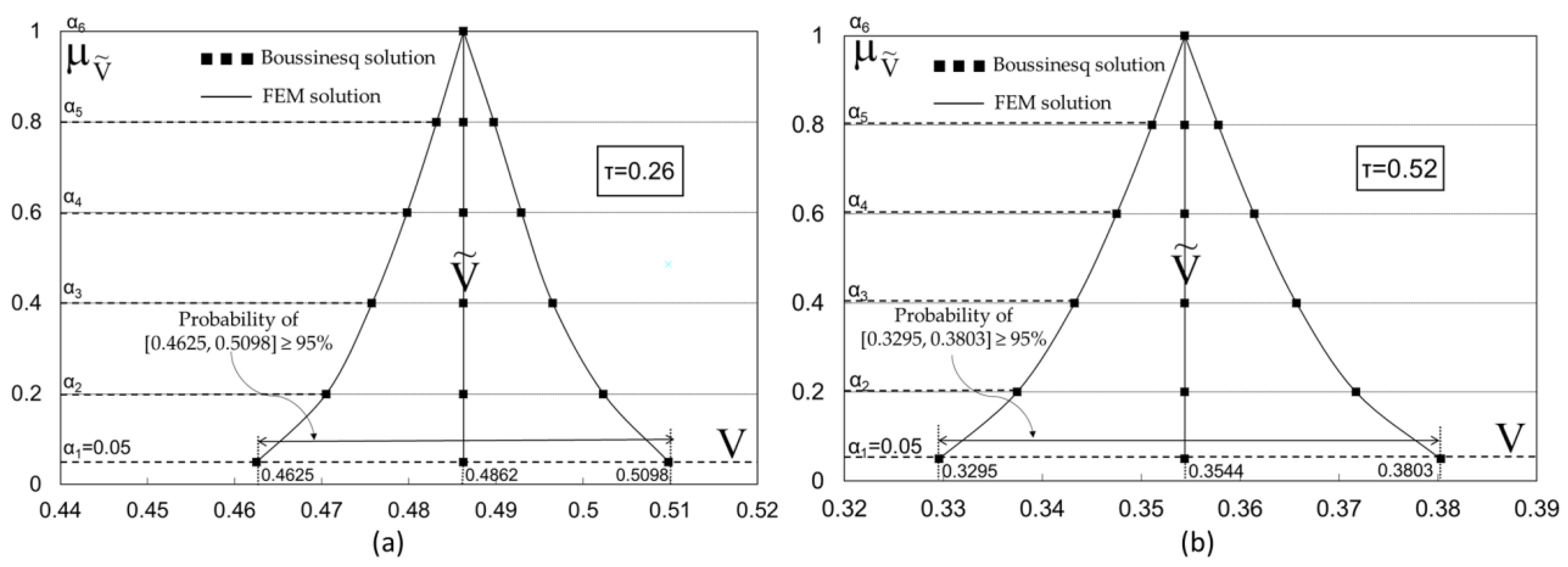
The integrated approach of FEM with the Boussinesq equation, validated against existing analytical and numerical solutions, provides a comprehensive understanding of groundwater recession in unconfined aquifers without precipitation. The developed FEM-Boussinesq model was validated against the Karadi numerical solution, which served as a valuable benchmark. The Karadi numerical solution, based on simplified assumptions, allows for a comparative analysis of the model’s performance in capturing the recession flow dynamics. In addition to the Karadi solution, we employed the Boussinesq exact analytical solution. The utilization of multiple solutions ensures a more robust verification process, offering confidence in the reliability of the model outcomes. Specifically, the proposed numerical scheme achieved significant performance against the exact solution of Boussinesq. By examining two different times, the mean absolute difference is 5.16 × 10⁻⁴ for τ = 0.26, and 1.75 × 10⁻³ for τ = 0.52 proved the closest in agreement with the results. The results against the Karadi numerical solution showed a lower performance than with the Boussinesq analytical solution; however, they are considered satisfactory, taking into account the assumptions by the Karadi method (see also Section 3.1) and that the solution is a numerical approximation.

In general, the proposed approach successfully captures the complex interplay between aquifer properties and recession flow dynamics, allowing for reliable predictions of groundwater outflow. The ability to quantify uncertainties and validate predictions against an analytical solution enhances the model’s reliability in guiding decision-making processes related to water resource management and sustainable groundwater use. These insights have direct implications for water resource management, particularly in regions where understanding recession flow is crucial for sustainable groundwater use. The validated model serves as a valuable decision-support tool, aiding in the development of effective water management strategies.

Moreover, the importance of the Boussinesq equation and its use in different fields reinforces the findings of the current research and the use of the proposed methodology in other practical applications. In this context, the proposed fuzzy FEM scheme could be used, for example, in geotechnical engineering to analyze the behavior of soils under different loading conditions. The proposed approach can indirectly enhance the accuracy of predictions regarding soil settlement, bearing capacity, and stability analysis of foundation and retaining structures. This can lead to more reliable designs and safer construction practices. Another very useful practical application of the proposed methodology could be in civil infrastructure and specifically in the design of dams, embankments, and underground tunnels where the knowledge of the groundwater flow, including the uncertainties, is considered more than necessary for successful and efficient construction projects. Also, undoubtedly, in drainage projects, the proposed approach can result in a more accurate calculation of the drain spacing as mainly the knowledge of hydraulic conductivity and its uncertainties is considered very important for determining the groundwater table, which mostly affects the drain spacing.

4.4. Limitations and Future Perspectives

Significant results were obtained during this research; however, there are certain limitations that should be addressed. The proposed approach offers a promising avenue for improving the accuracy and reliability of recession flow modeling.

Regarding the physical problem, it is important to acknowledge that the Karadi solution assumes steady-state boundary and initial conditions and homogeneous aquifer properties, which may not fully represent the complexity of real-world aquifer systems. Thus, challenges remain in accurately characterizing subsurface heterogeneity and dynamic changes in soil properties over time. This limitation emphasizes the need for continued efforts to refine both numerical and analytical approaches for recession flow modeling. Future research should focus on refining the solutions by incorporating advanced geostatistical methods and real-time monitoring data to improve their predictive accuracy under varying hydrological conditions.

Furthermore, it is essential to acknowledge the computational demands associated with Fuzzy FEM. The introduction of fuzzy logic also introduces additional computational complexity, and further research is needed to optimize the method for large-scale simulations. Additionally, the choice of membership functions and fuzzy rules plays a crucial role in the accuracy of the results, necessitating a thorough sensitivity analysis to identify the most suitable configurations while to advance the applicability of the proposed methodology, further research is recommended to explore alternative fuzzy logic formulations and investigate their impact on the accuracy and efficiency of the Fuzzy FEM-Boussinesq model. Moreover, ignoring the great performance of the fuzzy scheme, an additional stability analysis of the proposed fuzzy numerical scheme should be investigated in the future in order to prove whether the model is unconditionally stable or otherwise to determine its constraints. In addition, the inclusion of the uncertainties of the initial and boundary conditions coupled with the uncertainties of the parameters K and S could be future research but with a detailed investigation in order for the overall degree of uncertainty to be at normal levels and the results to be interpretable.

Lastly, to further refine and validate the model’s applicability to real-world conditions, integrating field observations, such as groundwater level measurements, subsurface geophysical data, and discharge records, is essential. This integration will not only contribute to continuous model refinement but also ensure its relevance in diverse hydrogeological settings.

5. Conclusions

In conclusion, the inclusion of uncertainties, particularly in hydraulic conductivity and porosity, is critical for advancing groundwater flow modeling. Embracing fuzzy approaches and ensemble modeling techniques provides a path forward for improving the reliability and accuracy of predictions, empowering stakeholders to make informed decisions in the sustainable management of groundwater resources.

The application of the Fuzzy Finite Element Method (FFEM) in modeling recession flow within unconfined aquifers without precipitation has proven effective in addressing the inherent uncertainties associated with aquifer properties. Specifically, in the current research, the application of our proposed solution to real cases as well as to the Boussinesq analytical solution has proved that the present numerical solution using the FEM method is in agreement with the Karadi et al. numerical method and in close agreement with the Boussinesq analytical method, and in addition, proves the accuracy and reliability of the new fuzzy numerical method. In addition, it was observed to be easy and simple to calculate in comparison to other methods without affecting the accuracy of the results, especially using the method of nondimensional time ${\tau }_{{\alpha }_i}$ for every α-cut.

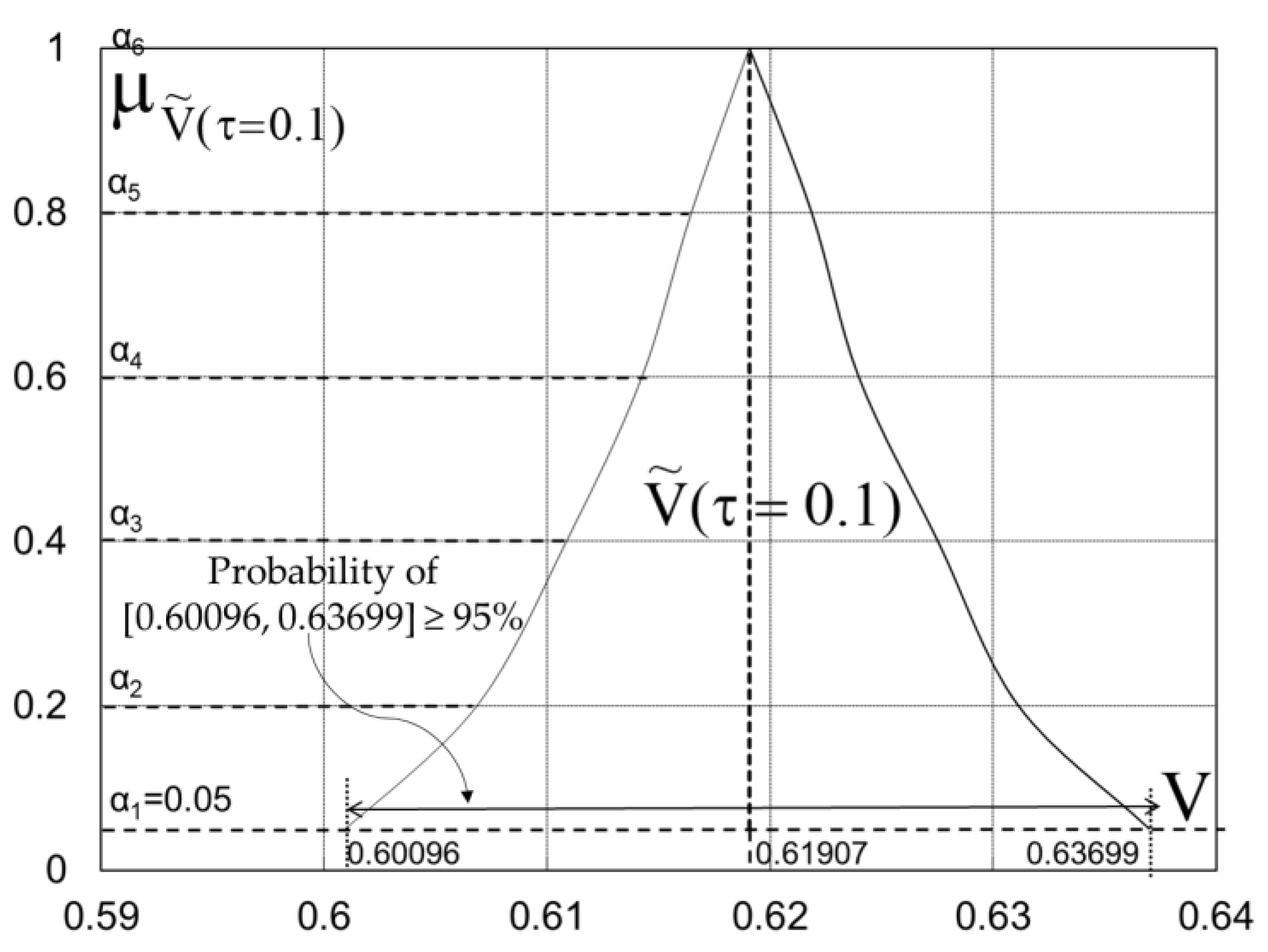
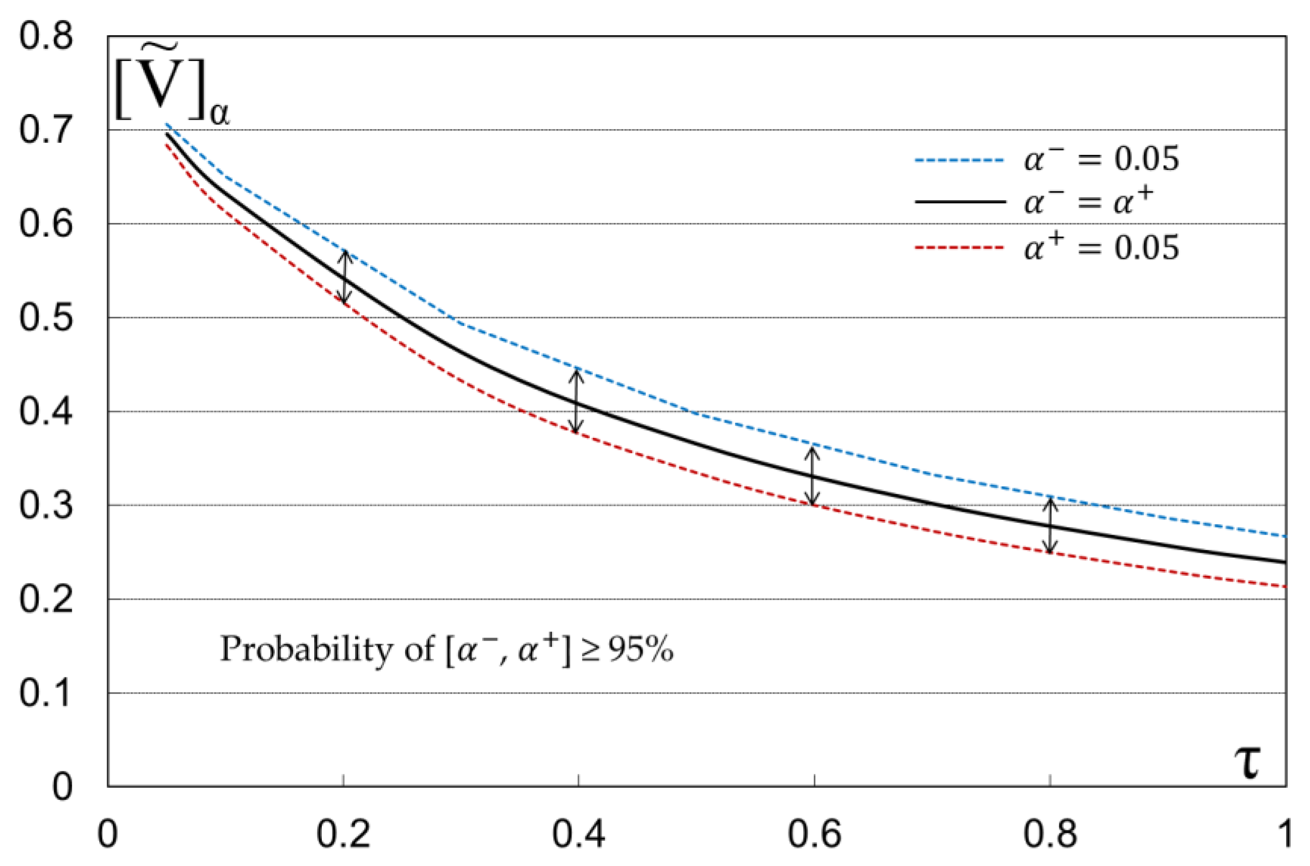
Furthermore, it should be noted that with the aid of the possibility theory, fuzzy estimators for different hydraulic parameters are possible. Therefore, for practical cases, such as irrigation, drainage, and water resources projects with uncertainties, the engineers and designers could now have a better idea of the real physical conditions. That is, knowing the confidence intervals of the crisp value of these hydraulic parameters with a certain strong probability, they can make the right decision.

By addressing uncertainties and leveraging analytical benchmarks, this research contributes to advancing hydrological modeling and underscores the practical implications for sustainable aquifer management, particularly concerning water discharge during recession periods.

In the future, our research could be oriented to present certain fuzzy FEM algorithms, which will optimize the method for large-scale simulations by insertion other more flexible Finite Elements (e.g., triangular) and presentation of a complete stability analysis with the von Neumann method. This algorithm will integrate field observations such as groundwater level measurements, subsurface geophysical data, and discharge records. This integration will not only contribute to continuous model refinement but also ensure its relevance and its future application in diverse hydrogeological settings.

References

1. Boussinesq, J. Recherches Theoriques Sur l’ecoulement Des Nappes d’eau Infiltrees Dans Le Sol et Sur Le Debit Des Sources. J. Math. Pures Appl. 1904, 10, 5–78. [Google Scholar]
2. Polubarinova-Kochina, P.Y. On a Non-Linear Differential Equation Occurring in Seepage Theory. DAN 1948, 36. [Google Scholar]
3. Polubarinova-Kochina, P.Y. On Unsteady Motions of Groundwater during Seepage from Water Reservoirs. P.M.M. (Prinkladaya Mat. I Mekhanica) 1949, 13. [Google Scholar]
4. Polubarinova-Kochina, P.Y. Theory of Groundwater Movement, 2015th ed.; Princeton University Press: Princeton, NJ, USA, 2015. [Google Scholar]
5. Tolikas, P.K.; Sidiropoulos, E.G.; Tzimopoulos, C.D. A Simple Analytical Solution for the Boussinesq One-Dimensional Groundwater Flow Equation. Water Resour. Res. 1984, 20, 24–28. [Google Scholar] [CrossRef]
6. Lockington, D.A. Response of Unconfined Aquifer to Sudden Change in Boundary Head. J. Irrig. Drain. Eng. 1997, 123, 24–27. [Google Scholar] [CrossRef]
7. Moutsopoulos, K.N. The Analytical Solution of the Boussinesq Equation for Flow Induced by a Step Change of the Water Table Elevation Revisited. Transp. Porous Media 2010, 85, 919–940. [Google Scholar] [CrossRef]
8. Basha, H.A. Traveling Wave Solution of the Boussinesq Equation for Groundwater Flow in Horizontal Aquifers. Water Resour. Res. 2013, 49, 1668–1679. [Google Scholar] [CrossRef]
9. Chor, T.; Dias, N.L.; de Zárate, A.R. An Exact Series and Improved Numerical and Approximate Solutions for the Boussinesq Equation. Water Resour. Res. 2013, 49, 7380–7387. [Google Scholar] [CrossRef]
10. Hayek, M. Accurate Approximate Semi-Analytical Solutions to the Boussinesq Groundwater Flow Equation for Recharging and Discharging of Horizontal Unconfined Aquifers. J. Hydrol. 2019, 570, 411–422. [Google Scholar] [CrossRef]
11. Khan, H.; Farooq, U.; Shah, R.; Baleanu, D.; Kumam, P.; Arif, M. Analytical Solutions of (2+Time Fractional Order) Dimensional Physical Models, Using Modified Decomposition Method. Appl. Sci. 2019, 10, 122. [Google Scholar] [CrossRef]
12. Shah, R.; Khan, H.; Kumam, P.; Arif, M. An Analytical Technique to Solve the System of Nonlinear Fractional Partial Differential Equations. Mathematics 2019, 7, 505. [Google Scholar] [CrossRef]
13. Rashid, S.; Khalid, A.; Sultana, S.; Hammouch, Z.; Shah, R.; Alsharif, A.M. A Novel Analytical View of Time-Fractional Korteweg-De Vries Equations via a New Integral Transform. Symmetry 2021, 13, 1254. [Google Scholar] [CrossRef]
14. Iqbal, N.; Akgül, A.; Shah, R.; Bariq, A.; Mossa Al-Sawalha, M.; Ali, A. On Solutions of Fractional-Order Gas Dynamics Equation by Effective Techniques. J. Funct. Spaces 2022, 2022, 3341754. [Google Scholar] [CrossRef]
15. Tzimopoulos, C.; Papadopoulos, K.; Evangelides, C.; Spyrides, A. Recharging and Discharging of Unconfined Aquifers. Case of Nonlinear Boussinesq Equation. In Proceedings of the Eighth International Conference on Environmental Management,Engineering, Planning and Economics (CEMEPE 2021) and SECOTOX Conference, CEMEPE 2021, Thessaloniki, Greece, 22 June 2021; pp. 74–80. [Google Scholar]
16. Wiedeburg, O. Ueber Die Hydrodiffusion. Ann. Phys. 1890, 277, 675–711. [Google Scholar] [CrossRef]
17. Chen, Z.-X.; Bodvarsson, G.S.; Witherspoon, P.A.; Yortsos, Y.C. An Integral Equation Formulation for the Unconfined Flow of Groundwater with Variable Inlet Conditions. Transp. Porous Media 1995, 18, 15–36. [Google Scholar] [CrossRef]
18. Parlange, J.-Y.; Hogarth, W.L.; Govindaraju, R.S.; Parlange, M.B.; Lockington, D. On an Exact Analytical Solution of the Boussinesq Equation. Transp. Porous Media 2000, 39, 339–345. [Google Scholar] [CrossRef]
19. Telyakovskiy, A.S.; Braga, G.A.; Furtado, F. Approximate Similarity Solutions to the Boussinesq Equation. Adv. Water Resour. 2002, 25, 191–194. [Google Scholar] [CrossRef]
20. Pistiner, A. Similarity Solution to Unconfined Flow in an Aquifer. Transp. Porous Media 2008, 71, 265–272. [Google Scholar] [CrossRef]
21. Olsen, J.S.; Telyakovskiy, A.S. Polynomial Approximate Solutions of a Generalized Boussinesq Equation. Water Resour. Res. 2013, 49, 3049–3053. [Google Scholar] [CrossRef]
22. Bartlett, M.S.; Porporato, A. A Class of Exact Solutions of the Boussinesq Equation for Horizontal and Sloping Aquifers. Water Resour. Res. 2018, 54, 767–778. [Google Scholar] [CrossRef]
23. Tzimopoulos, C.; Papadopoulos, K.; Evangelides, C.; Papadopoulos, B. Fuzzy Solution to the Unconfined Aquifer Problem. Water 2018, 1, 54. [Google Scholar] [CrossRef]
24. Remson, I.; Hornberger, G.; Moltz, F. Numerical Methods in Subsurface Hydrology; Wiley-Interscience: Toronto, ON, Canada, 1971. [Google Scholar]
25. Tzimopoulos, C.; Terzidis, G. Écoulement Non Permanent Dans Un Sol Drainé Par Des Fossés Parallèles. J. Hydrol. 1975, 27, 73–93. [Google Scholar] [CrossRef]
26. Chávez, C.; Fuentes, C.; Zavala, M.; Brambila, F. Numerical Solution of the Boussinesq Equation. Application to the Agricultural Drainage. Afr. J. Agric. Res. 2011, 18, 4210–4222. [Google Scholar]
27. Bansal, R.K. Groundwater Fluctuations in Sloping Aquifers Induced by Time-Varying Replenishment and Seepage from a Uniformly Rising Stream. Transp. Porous Media 2012, 94, 817–836. [Google Scholar] [CrossRef]
28. Bansal, K.R. Approximate Analytical Solution of Boussinesq Equation in Homogeneous Medium with Leaky Base. Appl. Appl. Math. Int. J. (AAM) 2016, 11, 184–191. [Google Scholar]
29. Borana, R.N.; Pradhan, V.H.; Mehta, N. Numerical Solution of Boussinesq Equation Arising in One-Dimensional Infiltration Phenomenon by Using Finite Difference Method. Int. J. Res. Eng. Technol. 2013, 2, 202–209. [Google Scholar]
30. Bansal, R.K. Unsteady Seepage Flow over Sloping Beds in Response to Multiple Localized Recharge. Appl. Water Sci. 2017, 7, 777–786. [Google Scholar] [CrossRef]
31. Nguyen, T. Numerical and Analytical Analysis of Flow in Stratified Heterogeneous Porous Media. Master’s Thesis, University of Stavanger, Stavanger, Norway, 2018. [Google Scholar]
32. Samarinas, N.; Tzimopoulos, C.; Evangelides, C. Fuzzy Numerical Solution to Horizontal Infiltration. Int. J. Circuits Syst. Signal Process. 2018, 12, 326–332. [Google Scholar]
33. Samarinas, N.; Tzimopoulos, C.; Evangelides, C. Fuzzy Numerical Solution to the Unconfined Aquifer Problem under the Boussinesq Equation. Water Supply 2021, 21, 3210–3224. [Google Scholar] [CrossRef]
34. Samarinas, N.; Tzimopoulos, C.; Evangelides, C. An Efficient Method to Solve the Fuzzy Crank–Nicolson Scheme with Application to the Groundwater Flow Problem. J. Hydroinform. 2022, 24, 590–609. [Google Scholar] [CrossRef]
35. Courant, R. Variational Methods for the Solution of Problems of Equilibrium and Vibrations. Bull. Am. Math. Soc. 1943, 49, 1–23. [Google Scholar] [CrossRef]
36. Argyris, J.H. Energy Theorems and Structural Analysis. Aircr. Eng. Aerosp. Technol. 1954, 26, 383–394. [Google Scholar] [CrossRef]
37. Turner, M.J.; Clough, R.W.; Martin, H.C.; Topp, L.J. Stiffness and Deflection Analysis of Complex Structures. J. Aeronaut. Sci. 1956, 23, 805–823. [Google Scholar] [CrossRef]
38. Oden, J.T. Historical Comments on Finite Elements. In A History of Scientific Computing; ACM: New York, NY, USA, 1990; pp. 152–166. [Google Scholar]
39. Tzimopoulos, C. Solution de l’équation de Boussinesq Par Une Méthode Des Éléments Finis. J. Hydrol. 1976, 30, 1–18. [Google Scholar] [CrossRef]
40. Galerkin, B.G. Rods and Plates: Series in Some Questions of Elastic Equilibrium of Rods and Plates; National Technical Information Service: Springfield, VA, USA, 1968. [Google Scholar]
41. Frangakis, C.N.; Tzimopoulos, C. Unsteady Groundwater Flow on Sloping Bedrock. Water Resour. Res. 1979, 15, 176–180. [Google Scholar] [CrossRef]
42. Tzimopoulos, C.; Tolikas, P. Technical and theoretical aspects in artificial ground water recharge. ICID Bull. Int. Comm. Irrig. Drain. 1980, 29, 40–44. [Google Scholar]
43. Tber, M.H.; El Alaoui Talibi, M. A Finite Element Method for Hydraulic Conductivity Identification in a Seawater Intrusion Problem. Comput. Geosci. 2007, 33, 860–874. [Google Scholar] [CrossRef]
44. Mohammadnejad, T.; Khoei, A.R. An Extended Finite Element Method for Hydraulic Fracture Propagation in Deformable Porous Media with the Cohesive Crack Model. Finite Elem. Anal. Des. 2013, 73, 77–95. [Google Scholar] [CrossRef]
45. Yang, D.; Zhou, Y.; Xia, X.; Gu, S.; Xiong, Q.; Chen, W. Extended Finite Element Modeling Nonlinear Hydro-Mechanical Process in Saturated Porous Media Containing Crossing Fractures. Comput. Geotech. 2019, 111, 209–221. [Google Scholar] [CrossRef]
46. Aslan, T.A.; Temel, B. Finite Element Analysis of the Seepage Problem in the Dam Body and Foundation Based on the Galerkin’s Approach. Eur. Mech. Sci. 2022, 6, 143–151. [Google Scholar] [CrossRef]
47. Ritz, W. Über Eine Neue Methode Zur Lösung Gewisser Variationsprobleme Der Mathematischen Physik. J. Die Reine Angew. Math. 1909, 1909, 1–61. [Google Scholar] [CrossRef]
48. Puri, M.L.; Ralescu, D.A. Differentials of Fuzzy Functions. J. Math. Anal. Appl. 1983, 91, 552–558. [Google Scholar] [CrossRef]
49. Hukuhara, M. Integration Des Applications Measurables Dont La Valeur Est Un Compact Convexe. Funkc. Ekvacioj 1967, 10, 205–233. [Google Scholar]
50. Kaleva, O. Fuzzy Differential Equations. Fuzzy Sets Syst. 1987, 24, 301–307. [Google Scholar] [CrossRef]
51. Seikkala, S. On the Fuzzy Initial Value Problem. Fuzzy Sets Syst. 1987, 24, 319–330. [Google Scholar] [CrossRef]
52. Vorobiev, D.; Seikkala, S. Towards the Theory of Fuzzy Differential Equations. Fuzzy Sets Syst. 2002, 125, 231–237. [Google Scholar] [CrossRef]
53. O’Regan, D.; Lakshmikantham, V.; Nieto, J.J. Initial and Boundary Value Problem for Fuzzy Differential Equations. Nonlinear Anal. 2003, 54, 405–415. [Google Scholar] [CrossRef]
54. Nieto, J.J.; Rodríguez-López, R. Bounded Solutions for Fuzzy Differential and Integral Equations. Chaos Solitons Fractals 2006, 27, 1376–1386. [Google Scholar] [CrossRef]
55. Diamond, P. Brief Note on the Variation of Constants Formula for Fuzzy Differential Equations. Fuzzy Sets Syst. 2002, 129, 65–71. [Google Scholar] [CrossRef]
56. Bede, B.; Gal, S.G. Generalizations of the Differentiability of Fuzzy-Number-Valued Functions with Applications to Fuzzy Differential Equations. Fuzzy Sets Syst. 2005, 151, 581–599. [Google Scholar] [CrossRef]
57. Stefanini, L. A Generalization of Hukuhara Difference and Division for Interval and Fuzzy Arithmetic. Fuzzy Sets Syst. 2010, 161, 1564–1584. [Google Scholar] [CrossRef]
58. Allahviranloo, T.; Gouyandeh, Z.; Armand, A.; Hasanoglu, A. On Fuzzy Solutions for Heat Equation Based on Generalized Hukuhara Differentiability. Fuzzy Sets Syst. 2015, 265, 1–23. [Google Scholar] [CrossRef]
59. Rodríguez Pérez, Á.M.; Rodríguez, C.A.; Olmo Rodríguez, L.; Caparros Mancera, J.J. Revitalizing the Canal de Castilla: A Community Approach to Sustainable Hydropower Assessed through Fuzzy Logic. Appl. Sci. 2024, 14, 1828. [Google Scholar] [CrossRef]
60. Rodríguez-Pérez, Á.M.; Rodríguez, C.A.; Márquez-Rodríguez, A.; Mancera, J.J.C. Viability Analysis of Tidal Turbine Installation Using Fuzzy Logic: Case Study and Design Considerations. Axioms 2023, 12, 778. [Google Scholar] [CrossRef]
61. Tzimopoulos, C.; Evangelides, C.; Vrekos, C.; Samarinas, N. Fuzzy Linear Regression of Rainfall-Altitude Relationship. Proceedings 2018, 2, 636. [Google Scholar] [CrossRef]
62. Samarinas, N.; Evangelides, C. Discharge Estimation for Trapezoidal Open Channels Applying Fuzzy Transformation Method to a Flow Equation. Water Supply 2021, 21, 2893–2903. [Google Scholar] [CrossRef]
63. Tzimopoulos, C.; Papadopoulos, K.; Papadopoulos, B.; Samarinas, N.; Evangelides, C. Fuzzy Solution of Nonlinear Boussinesq Equation. J. Hydroinform. 2022, 24, 1127–1147. [Google Scholar] [CrossRef]
64. Cherki, A.; Plessis, G.; Lallemand, B.; Tison, T.; Level, P. Fuzzy Behavior of Mechanical Systems with Uncertain Boundary Conditions. Comput. Methods Appl. Mech. Eng. 2000, 189, 863–873. [Google Scholar] [CrossRef]
65. Behera, D.; Chakraverty, S. Fuzzy Finite Element Based Solution of Uncertain Static Problems of Structural Mechanics. Int. J. Comput. Appl. 2013, 59, 69–75. [Google Scholar] [CrossRef]
66. Ranjit, D.K.; Roy, T.K. Fuzzy Finite Element Method Applied to Euler-Bernoulli Beam Problem. Int. J. Math. Trends Technol. 2018, 53, 304–320. [Google Scholar] [CrossRef]
67. Rodríguez, C.A.; Rodríguez-Pérez, Á.M.; López, R.; Hernández-Torres, J.A.; Caparrós-Mancera, J.J. A Finite Element Method Integrated with Terzaghi’s Principle to Estimate Settlement of a Building Due to Tunnel Construction. Buildings 2023, 13, 1343. [Google Scholar] [CrossRef]
68. Karadi, G.; Krizek, R.J.; Elnaggar, H. Unsteady Seepage Flow between Fully-Penetrating Trenches. J. Hydrol. 1968, 6, 417–430. [Google Scholar] [CrossRef]
69. Oden, J.T. Finite Elements of Nonlinear Continua; Dover Publications: Mineola, NY, USA, 1972. [Google Scholar]
70. Thomas, L.H. Elliptic Problems in Linear Differential Equations over a Network; Watson Sci Lab Report Columbia University: New York, NY, USA, 1949. [Google Scholar]
71. Negoiţă, C.V.; Ralescu, D.A. Applications of Fuzzy Sets to Systems Analysis; Birkhäuser: Basel, Switzerland, 1975. [Google Scholar]
72. Goetshel, R.; Voxman, W. Elementary Fuzzy Calculus. Fuzzy Sets Syst. 1986, 18, 31–43. [Google Scholar] [CrossRef]
73. Bede, B.; Stefanini, L. Generalized Differentiability of Fuzzy-Valued Functions. Fuzzy Sets Syst. 2013, 230, 119–141. [Google Scholar] [CrossRef]
74. Khastan, A.; Nieto, J.J. A Boundary Value Problem for Second Order Fuzzy Differential Equations. Nonlinear Anal. Theory Methods Appl. 2010, 72, 3583–3593. [Google Scholar] [CrossRef]
75. Dubois, D.; Foulloy, L.; Mauris, G.; Prade, H. Probability-Possibility Transformations, Triangular Fuzzy Sets, and Probabilistic Inequalities. Reliab. Comput. 2004, 10, 273–297. [Google Scholar] [CrossRef]
76. Mylonas, N. Applications in Fuzzy Statistic and Approximate Reasoning. Ph.D. Thesis, Dimoktritos University of Thrace, Xanthi, Greece, 2022. [Google Scholar]
77. Tzimopoulos, C.; Samarinas, N.; Papadopoulos, K.; Evangelides, C. Fuzzy Unsteady-State Drainage Solution for Land Reclamation. Hydrology 2023, 10, 34. [Google Scholar] [CrossRef]
78. Richard, G.; Sillon, J.F.; Marloie, O. Comparison of Inverse and Direct Evaporation Methods for Estimating Soil Hydraulic Properties under Different Tillage Practices. Soil. Sci. Soc. Am. J. 2001, 65, 215–224. [Google Scholar] [CrossRef]
79. Richard, G.; Cousin, I.; Sillon, J.F.; Bruand, A.; Guérif, J. Effect of Compaction on the Porosity of a Silty Soil: Influence on Unsaturated Hydraulic Properties. Eur. J. Soil. Sci. 2001, 52, 49–58. [Google Scholar] [CrossRef]
80. Anderskouv, K.; Surlyk, F. The Influence of Depositional Processes on the Porosity of Chalk. J. Geol. Soc. Lond. 2012, 169, 311–325. [Google Scholar] [CrossRef]
81. Carbillet, L.; Heap, M.J.; Baud, P.; Wadsworth, F.B.; Reuschlé, T. The Influence of Grain Size Distribution on Mechanical Compaction and Compaction Localization in Porous Rocks. J. Geophys. Res. Solid. Earth 2022, 127, e2022JB025216. [Google Scholar] [CrossRef]
82. Van Lopik, J.H.; Snoeijers, R.; van Dooren, T.C.G.W.; Raoof, A.; Schotting, R.J. The Effect of Grain Size Distribution on Nonlinear Flow Behavior in Sandy Porous Media. Transp. Porous Media 2017, 120, 37–66. [Google Scholar] [CrossRef]
83. Sihag, P. Prediction of Unsaturated Hydraulic Conductivity Using Fuzzy Logic and Artificial Neural Network. Model. Earth Syst. Environ. 2018, 4, 189–198. [Google Scholar] [CrossRef]
84. More, S.B.; Deka, P.C. Estimation of Saturated Hydraulic Conductivity Using Fuzzy Neural Network in a Semi-Arid Basin Scale for Murum Soils of India. ISH J. Hydraul. Eng. 2018, 24, 140–146. [Google Scholar] [CrossRef]
85. Ross, J.; Ozbek, M.; Pinder, G.F. Hydraulic Conductivity Estimation via Fuzzy Analysis of Grain Size Data. Math. Geol. 2007, 39, 765–780. [Google Scholar] [CrossRef]
Figure 1. Definition sketch of the investigated problem.
Hydrology 11 00047 g001
Figure 2. Finite elements model: (a) global basis function, and (b) local basis function.
Hydrology 11 00047 g002
Figure 3. Fuzzy estimators of (a) K, (b) S, and (c) ratio K/S.
Hydrology 11 00047 g003
Figure 4. Boundary and initial conditions.
Hydrology 11 00047 g004
Figure 5. Groundwater levels H for different nondimensional time τ. Comparison of FEM method vs. Karadi et al. (1968) numerical scheme [68]. The bold black lines represent the α-cut = 1 while the other two lines are α (dash red line) and α+ (dash blue line) cuts.
Hydrology 11 00047 g005
Figure 6. Fuzzy estimator of outflow volume V for τ = 0.1.
Hydrology 11 00047 g006
Figure 7. Boussinesq initial curve and polynomial approximation H1, H2.
Hydrology 11 00047 g007
Figure 8. Groundwater levels H for different nondimensional time τ. Comparison of FEM method vs. Boussinesq analytical method. The bold lines represent the α-cut (α = 1), while the other two dash lines on either side represent the α-cuts (α, α+).
Hydrology 11 00047 g008
Figure 9. Fuzzy outflow volume V for different times.
Hydrology 11 00047 g009
Figure 10. Fuzzy estimator of outflow volume V for (a) τ = 0.26 and (b) τ = 0.52.
Hydrology 11 00047 g010