‘Teflon Basin’ or Not? A High-Elevation Catchment Transit Time Modeling Approach


1
Department of Geography, University of Innsbruck, 6020 Innsbruck, Austria
2
Chair of Hydrology, University of Freiburg, 79098 Freiburg, Germany
*
Author to whom correspondence should be addressed.
Hydrology 2019, 6(4), 92; https://0-doi-org.brum.beds.ac.uk/10.3390/hydrology6040092
Submission received: 30 August 2019
/
Revised: 11 October 2019
/
Accepted: 20 October 2019
/
Published: 22 October 2019
(This article belongs to the Special Issue Snow Hydrology: Monitoring and Modelling)
Abstract
:We determined the streamflow transit time and the subsurface water storage volume in the glacierized high-elevation catchment of the Rofenache (Oetztal Alps, Austria) with the lumped parameter transit time model TRANSEP. Therefore we enhanced the surface energy-balance model ESCIMO to simulate the ice melt, snowmelt and rain input to the catchment and associated δ18O values for 100 m elevation bands. We then optimized TRANSEP with streamflow volume and δ18O for a four-year period with input data from the modified version of ESCIMO at a daily resolution. The median of the 100 best TRANSEP runs revealed a catchment mean transit time of 9.5 years and a mobile storage of 13,846 mm. The interquartile ranges of the best 100 runs were large for both, the mean transit time (8.2–10.5 years) and the mobile storage (11,975–15,382 mm). The young water fraction estimated with the sinusoidal amplitude ratio of input and output δ18O values and delayed input of snow and ice melt was 47%. Our results indicate that streamflow is dominated by the release of water younger than 56 days. However, tracers also revealed a large water volume in the subsurface with a long transit time resulting to a strongly delayed exchange with streamflow and hence also to a certain portion of relatively old water: The median of the best 100 TRANSEP runs for streamflow fraction older than five years is 28%.
1. Introduction
High-elevation catchments were often seen as ’Teflon’-like basins [1], meaning that water input to the catchment immediately runs off as overland flow or fast subsurface flow with very limited subsurface interaction [2] and minimal infiltration, due to the permeability of bedrock typically assumed to be negligible [3]. The concept of how catchments retain water is becoming almost equally recognized as how catchments release water [4,5,6,7]. However, very recent studies mentioned the formerly unrecognized subsurface storage potential of mountain catchments [4,8,9], i.e., water is not only temporarily stored as snow and ice, but also in the soil, fractured bedrock, moraines, talus, alluvium, alluvial fans, permafrost, rock glaciers and rock slides [4,10,11,12,13]. This water contributes to streamflow by shallow to deep flow paths [3,14], both in periods with rain, snowmelt and ice melt input and in periods without water input to the catchment (i.e., when the catchment is in a frozen state [8]), and hence is an important contributor to streamflow. This subsurface water may play an important role in the alpine hydrologic cycle as shown by numerous studies in glacier-free and glacierized catchments [12,15,16,17,18,19,20]. Snowmelt, ice melt and rain recharge the subsurface storage, with snowmelt being the most important contributor in many mountain catchments worldwide [21,22]. The water volume and flow (the quotient is the transit time) thereby affect both, downstream water supply and quality [4,23].
Streamflow age is a crucial descriptor of catchment functioning, affecting the control of runoff generation, biogeochemical cycling and contaminant transport. It is defined as the elapsed time for water transmitted through the catchment from input to the stream at the outlet [23,24]. The transit time distribution (TTD) describes the age composition of a streamflow water sample, and can be inferred from seasonal tracer cycles with the convolution integral method by relating past tracer input (e.g., precipitation) to tracer output (e.g., streamflow) [23]. The mean transit time (MTT) thereby describes the average travel time for a water parcel from entering to leaving a catchment [23]. Dynamic storage controls streamflow dynamics (i.e., the runoff response), whereas mobile storage, also connected to streamflow, shows large differences in water age and controls transport in a catchment (i.e., the tracer response) [4]. An overview of perceptual storage terms in catchment hydrology and respective estimation methods can be found in Staudinger et al. [4]. The young water fraction (Fyw) is the proportion of streamflow below a certain threshold age (typically less than 3 months) and can be estimated by comparing fitted seasonal sine wave tracer cycles of catchment input and output [25,26].
Streamflow age (including Fyw) and subsurface storage studies were already conducted in catchments in a variety of environmental settings: in low mountain catchments, e.g., [27,28], in northern high-latitude catchments, e.g., [29,30], in high mountain catchments, whereby only a few were covered by a small percentage of glacier ice (<5%), e.g., [4,31,32], or in permafrost regions, e.g., [33]. Seeger and Weiler [32] combined a surface energy-balance model with a lumped parameter transit time model and reported MTTs of 0.6 to 10.5 years for five snow-dominated catchments in Switzerland. Staudinger et al. [4] revealed dynamic and mobile storages of approximately 100 to 500 mm and 1000 to 13,000 mm for four snow-dominated catchments in Switzerland (these were included in the analyses of [32]), respectively. Freyberg et al. [31] estimated a flow-weighted Fyw of 0.1 to 0.22 for the same Swiss catchments analyzed in [32]. A global study of 254 river systems revealed a flow-weighted mean Fyw of 0.34 with a threshold age of 2.3 ± 0.8 months, whereas almost all of the mountain rivers had a lower Fyw than the mean [11]. Freyberg et al. [31] tested the delayed effect of snowmelt during their application of the Fyw approach and found a significant difference in the amplitude of fitted seasonal tracer cycle of input water for only one out of 21 catchments compared to the method with a direct input of precipitation. They concluded that in their study catchments, Fyw values were not sensitive to the use of delayed input. Tetzlaff et al. [29] extended the traditional transit time estimation approach with a snow model that provides snow melt volume and isotope ratio and applied it in an Arctic catchment. They concluded that considering all available inflows (i.e., snow melt, soil ice thaw and rainfall) led to the best estimated transit time. Hence we hypothesize that the spatio-temporal variability of the water input in glacierized high-elevation catchments (i.e., especially the snow and ice melt volume and their isotope ratios) is important, which challenges the traditional transit time and Fyw approach (where rain is considered to contribute dominantly).
It can be concluded that studies addressing the Fyw, catchment TTD or storage estimates in catchments with >5% glacierized area are missing and estimates of the above-mentioned metrics are unknown, but high-elevation catchment storage (not snow and ice) may become even more important in terms of a changing climate and shrinking glaciers. The question arises how the occurrence of ice melt as a contributor and significant part of the water cycle affects the estimation of Fyw, catchment TTD and storage in glacierized high-elevation catchments. We make use of a model coupling approach in which we combine a surface energy-balance model to simulate the snow and ice melt volume and isotope ratio with a lumped parameter transit time model to estimate the catchment TTD and storage. Overall, we aim to identify the role of subsurface water (and storage) in a glacierized high-elevation catchment with the use of δ18O. Specifically, the objectives are:
- The estimation of catchment transit time and mobile storage by coupling of a surface energy-balance snow and ice melt model with a lumped parameter transit time model,
- The estimation of the Fyw with delayed input of snow and ice melt using the sine wave approach and,
- The comparison of the TTD and the Fyw.
2. Materials and Methods
2.1. Study Area
We conducted our study in the 35% glacierized high-elevation catchment Rofental (Figure 1), a LTSER site in the Austrian Alps (https://www.lter-austria.at/rofental/). The catchment (98 km2) ranges from approximately 1890 to 3770 m a.s.l. (mean elevation is 2930 m a.s.l.). The Rofenache is draining the catchment and has a distinct glacial regime with a mean flow of 4.6 m3 s−1 (1971–2013) at the outlet in Vent (1891 m a.s.l., 46.85722° N, 10.91083° E). Mean 7-day annual minimum flow, mean flow and mean annual peak flow for the period 2014 to 2017 are 0.43, 3.93 and 24.59 mm d−1, respectively.
Detailed site descriptions, including various climatic and hydrologic characteristics, can be found in Schmieder et al. [34] or in Strasser et al. [35]. Several cryospheric, hydrologic and geodetic studies have been conducted in the catchment and data sets from more than 150 years ago up to very recently are freely available [35]. Hydrologic tracer studies have been conducted intensively during the International Hydrological Decade (1965–1974) [36] and since 2014 [37]. Strasser et al. [35] provide a detailed overview about the research history in the Rofental. Figure 1 shows the catchment, as well as the water sampling and ‘Austrian Network of Isotopes in Precipitation and Surface Waters’ (ANIP) sites used in this publication.
2.2. Data
We used daily runoff data (streamflow was measured at the gauging station in Vent) within this study. Hourly meteorological variables (air temperature, precipitation amount, relative humidity, wind speed and global radiation) were measured at various stations (see [38,39] for more details) and were interpolated with the hydroclimatological modeling system AMUNDSEN [38,40] to 50 m pixel resolution grids. For further model input in this study, these grids were aggregated to 100 m elevation bands (n = 19) in daily resolution.
Streamflow isotope samples (n = 98) were collected in non-equitemporal intervals for 2014 to 2016 (grab samples) and in daily intervals for 2017 (automatic water sampler) at the gauging station at Vent. The water samples were mostly collected during daytime in the ablation season. For days with multiple samples a flow-weighted mean was calculated. The sampling time is documented in Table S3.
Monthly long-term precipitation isotope data of the surrounding ANIP stations (Figure 1) were used to calculate monthly lapse rates of δ18O. These lapse rates were applied to the ANIP station in Obergurgl (1942 m a.s.l., 46.866667° N, 11.024444° E, see Figure 1) to regionalize the δ18O of precipitation registered there (100 m elevation bands). The Obergurgl δ18O values of precipitation were assumed to be transferable to the catchment since regression of precipitation δ2H values from Vent and Obergurgl revealed a very high correlation (R2 = 0.89) for the years 1972 to 1975 [41]. Lapse rate data (Tables S1 and S2) and the regression plot (Figure S1) can be found in the supplement.
Snowmelt isotopic data was not derived from sampling, but was modeled from precipitation isotopic data (as described in Section 2.3). Supraglacial meltwater (hereafter ice melt) was sampled on Hochjochferner (n = 72) at an elevation of approximately 2700 m a.s.l. at various temporal (including sub-daily and month-to month) and spatial resolutions (spatial extent: 100s of meter). Samples have been collected when most of the glacier was snow-free.
The isotope data (not ANIP data) has been partially described already [10,34,37,42]. Water samples were stored cold and dark before analyses with cavity ring-down spectroscopy (Picarro Inc., Santa Clara, CA, USA). The accuracy, indicated by the standard deviation of at least six repeated measurements, was ≤0.1‰. 18O/16O isotope ratios are reported as δ18O (in ‰) relative to the Vienna standard mean ocean water (VSMOW). The modeling workflow is described in the following sections and a schematic overview is displayed in Figure S2.
2.3. The Surface Energy-Balance Model ESCIMO
We used the modified version [32] of the surface energy-balance model ESCIMO [43] to simulate the rain, snow and ice melt input fluxes and the respective δ18O values for 100 m elevation bands. ESCIMO has been successfully applied at low and high mountain sites, e.g., [44,45]. A similar setup like in our study has been already applied successfully [4,31,32], where snow melt δ18O was simulated as the weighted average of individual snowfall events without addressing isotopic fractionation explicitly. δ18O of ice melt was not considered in those studies since the glacierized area of the test catchments was <5%. ESCIMO inputs are meteorological variables as described in Section 2.2 and δ18O in precipitation. We enhanced ESCIMO to simulate ice melt volumes. Therefore ESCIMO is enabled to calculate melt rates when snow water equivalent is zero. Potential ice melt rates are then multiplied with the glacierized fraction of the respective elevation band to calculate semi-distributed ice melt input fluxes. We ascribed the simulated ice melt volume in each elevation band a δ18O value to account for spatial variability as done in similar studies, e.g., [46]. This value is the median of the measured ice melt δ18O values at the elevation of 2700 m a.s.l. (−15.4‰) and changes according to the mean lapse rate (−0.221‰/100 m) of δ18O in precipitation between November and May (as described in Section 2.2). The temporal variability of δ18O in ice melt was not considered.
2.4. The Lumped Parameter Transit Time Model TRANSEP
The lumped parameter transit time model TRANSEP [47] was used to estimate the time-invariant TTD and response time distribution (RTD), as well as the dynamic and mobile storage. TRANSEP has been applied successfully in catchments with various environmental conditions, e.g., [28,48,49], and also in high mountain catchments, e.g., [32]. ESCIMO output data (i.e., catchment water input PE: the sum of rain, snow and ice melt volumes; CE: the amount-weighted δ18O value of rain, snow and ice melt) were spatially aggregated to the catchment scale and used as input data for TRANSEP. The model was run at a daily resolution.
TRANSEP simulates discharge for each time step t with Equation (1), where g(τR) is the transfer function for discharge (Equation (2)) with τR, φ, τf and τs being the response time, fraction of fast reservoir and the MTT of the fast and the slow reservoir, respectively. Equation (2) is calibrated with measured streamflow data.
δ18O values of streamflow are simulated with Equation (3), where h(τT) is the transfer function for streamflow δ18O (Equation (4)), with τT being the transit time, and α and β being the shape and scale parameter, respectively. Equation (4) is calibrated with measured streamflow δ18O.
After initial testing, we chose the two parallel linear reservoirs (TPLR) for the discharge transfer function (i.e., Equation (2)) and the gamma distribution (GM) for the tracer transfer function (i.e., Equation (4)). These gave the best results with respect to the objective function.
To optimize the simulated discharge, we used a scaled variant [50] of the Kling-Gupta efficiency (KGE) [51]. It emphasizes the flow variability term (α): A two times higher weight compared to the bias (β) and the correlation term (r) was used. Therefore we maximized KGEQ (Equation (5)) for the period 2014 to 2017.
We optimized the simulated δ18O in streamflow by minimizing OFC (Equation (6)), using the KGE (with the same weighting as used for optimizing discharge). We split the time series into two periods according to the temporal sampling intervals (as described in Section 2.2): (1) low frequency period (lf) 2014–2016 and (2) high-frequency period (hf) 2017. For a simpler readability we reported the KGE with standard scaling hereafter.
For the optimization procedure we used a Monte Carlo simulation with 10,000 runs and uniformly distributed parameters. The initial parameter ranges for Equations (2) and (4) were φ [0.1,0.9], τf [0.5,15], τs [20,600], α [0.01,1] and β [1·10−8,3·104]. The best 1% of the runs (n = 100), with the highest value of KGEQ (Equation (5)) and the lowest value of OFC (Equation (6)) were considered for further analyses. The mean response time (MRT) and MTT were calculated with Equations (7) and (8).
Dynamic and mobile storage has been calculated by multiplying mean flow with the MRT and the MTT, respectively. Table S3 includes the observed runoff and δ18O value of streamflow, as well as the catchment water input and its respective δ18O value as modeled with ESCIMO.
2.5. Estimating the Young Water Fraction with the Sine Wave Approach
We calculated the Fyw following Kirchner [25] and Stockinger et al. [28]. First, seasonal δ18O cycles in input water and streamflow (Equations (9) and (10)) were fitted by multiple linear regression with an iteratively reweighted least squares algorithm (provided by Freyberg et al. [31]). CE and CS are the δ18O values of input water as modeled with ESCIMO and measured streamflow at time t, and were weighted with PE and observed runoff, respectively. aE, bE, kE, aS, bS and kS are the cosine and sine coefficient parameter and the vertical shift for input water and streamflow, respectively. f is the frequency (1/365.25).
The amplitudes (A) of the seasonal δ18O cycles of input water and streamflow (Equations (11) and (12)) are calculated as:
and the phases ϕE and ϕS (in rad) are calculated as:
We iteratively solved Equation (15) to calculate the shape parameter α of a gamma distribution.
The scale parameter β (Equation (16)) was calculated as:
By solving Equation (17) we calculated the threshold age τyw that defines Fyw with water younger than this value. Fyw is calculated with Equation (18) using the lower incomplete gamma function Γ(τyw,α,β).
We call this Fyw estimation approach ‘delayed daily Fyw’ since it accounts for the delayed contribution of snow and ice melt as simulated with ESCIMO. We also calculated the non-delayed monthly Fyw and the delayed monthly Fyw for comparison reasons. For the non-delayed monthly Fyw we used the input precipitation data as used for the ESCIMO simulation (see in Section 2.2) and aggregated it to the monthly resolution (because the ANIP data used for the isotope interpolation is in monthly resolution). This approach does neither account for any temporal storage as snow and ice, nor the delayed release from snow and ice. Since resolution may play a role in estimating the Fyw [28], we also estimated the delayed monthly Fyw to compare the results related to the effect of the delayed and the non-delayed input (both then at the same temporal resolution). For the delayed monthly Fyw we simply aggregated PE (sum) and CE (volume-weighted average) and performed the analyses in monthly resolution.
We calculated the uncertainty in all three Fyw approaches by fitting each sine wave 10,000 times. For this, we used randomly sampled sine and cosine coefficient parameter (a and b in Equations (9) and (10)) out of a normal distribution with the mean being the respective parameter as estimated with Equations (9)–(18), and a standard deviation equal to the standard error of the multiple linear regression analyses. Fit statistics, as well as regression parameter and their standard errors can be found in Table S4.
3. Results
3.1. δ18O Values of Various Water Types in the Rofental for the Period 2014 to 2017
Figure 2 shows boxplots of the δ18O values in rain, snow melt, ice melt and streamflow for the period 2014 to 2017. Rain and snow melt δ18O values were simulated with ESCIMO (catchment scale). The boxplots reveal a high temporal variability in both, rain and snow melt, with snow melt having a markedly lower median (−15.6‰) than rain (−11.4‰). Rain δ18O values were significantly different from snowmelt, ice melt and streamflow δ18O (Kruskal-Wallis test: p < 0.001). The ice melt boxplot represents the time-invariant values of each elevation band derived from measured δ18O values and interpolated as described in Section 2.2 and hence displays the spatial variability in Figure 2. The median (−15.4‰) was slightly higher and the interquartile range is damped compared to snowmelt. Streamflow represents the measured data (temporal variability) as used for the optimization of TRANSEP, had a median of −14.9‰ and was damped compared to the rain and snow melt input.
3.2. Flux and δ18O of Water Input into the Rofenache Catchment
Monthly isotopic lapse rates were estimated using surrounding long-term data from ANIP stations. R2 for monthly δ18O-elevation relationships ranged from 0.46 to 0.94 (Table S2). The lapse rates showed seasonality with steeper gradients in winter (March: −0.265‰/100 m) and flatter gradients in summer (July: −0.112‰/100 m). Further information is provided in the supplement (Tables S1 and S2).
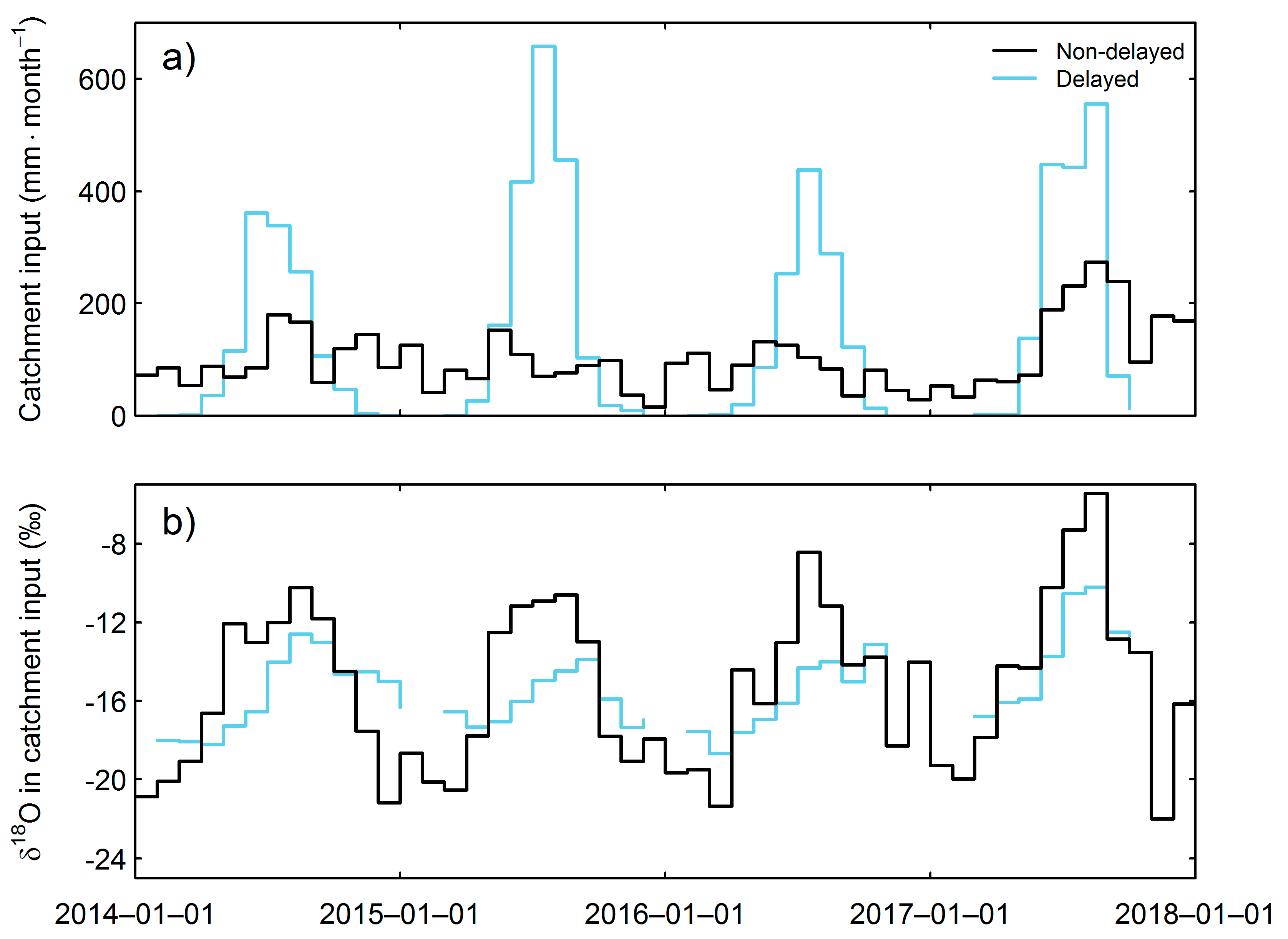
The interpolated precipitation input (non-delayed) into the catchment (black line in Figure 3a), i.e., the sum of snowfall and rain, reveals a slight seasonal cycle with values of about 100 mm month−1. The delayed liquid water input into the catchment (light blue line in Figure 3a), i.e., the sum of rain, snow and ice melt modeled with ESCIMO, had a strong seasonal characteristic with close to or zero input during the winter months (December to March) and very high inputs >350 mm month−1 during the peak ablation period (June to August).
The δ18O value of catchment input shows a strong seasonality for both, the delayed ESCIMO catchment input (PE) and the interpolated non-delayed precipitation catchment input (light blue and black lines in Figure 3b). The delayed monthly δ18O values (CE) ranged from −18.7‰ to −10.2‰ and exhibited more damped amplitude than the non-delayed δ18O values (−22.0‰ to −5.5‰).
3.3. Runoff and δ18O in Streamflow of the Rofenache at the Gauging Station in Vent
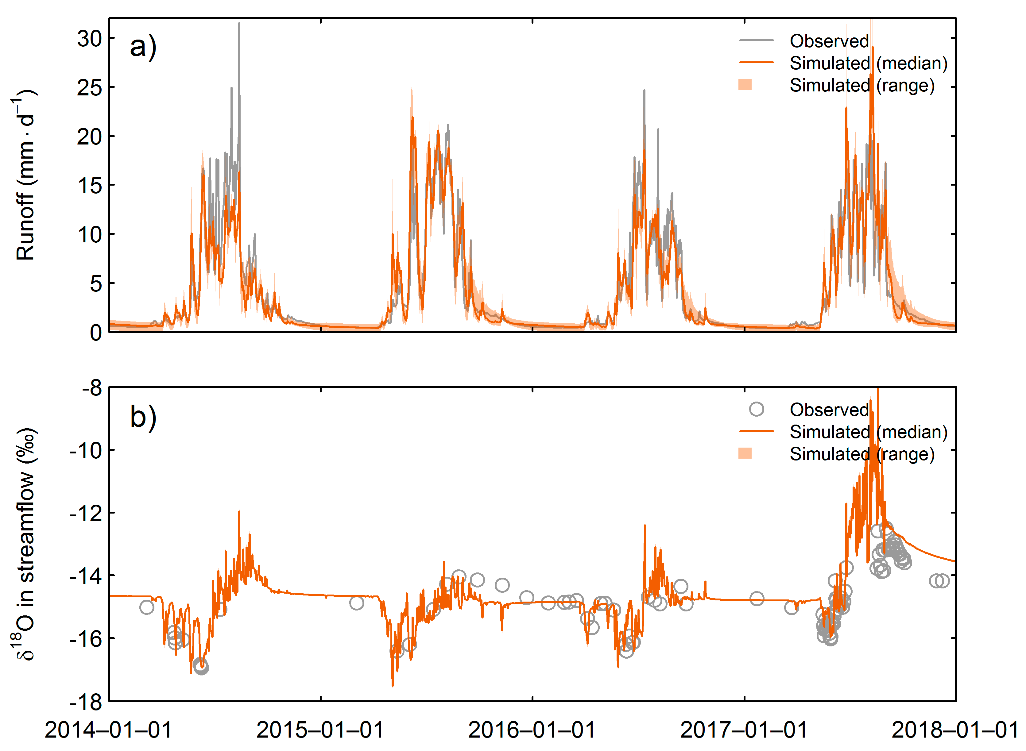
Figure 4a shows the observed and simulated (with TRANSEP) daily runoff for the period 2014 to 2017 for the gauging station in Vent (1891 m a.s.l.). Mean 7-day annual minimum flow, mean flow and mean annual peak flow of the simulation runs (median of best 100 runs) were 0.46, 3.79 and 21.47 mm d−1, respectively. Both, observed and simulated runoff show a very strong seasonality, with high flows and high day-to-day variability during the ablation period (>10 mm d−1 from June to August) and low flows concomitant with low day-to-day variability during the winter baseflow period (<1 mm d−1 from December to March). The KGE for runoff (best 100 runs) was 0.97.
Observed and simulated streamflow δ18O (median of best 100 runs) also reveal a strong seasonality with the highest values during late summer and the lowest values during the peak snowmelt period in late spring (Figure 4b). The simulated δ18O values ranged from −17.6‰ to −7.8‰ with respect to the best 100 TRANSEP simulations (the orange band in Figure 4b is very thin and covered by the orange line). The range of the 98 observed streamflow δ18O values was −16.9‰ to −12.5‰. During winter baseflow conditions (December to March), the simulated δ18O values with a range of −15.3‰ to −13.4‰ (median of the best 100 TRANSEP runs) were close to the median of the observed ones for the whole period (−14.9‰) and reflected a small day-to-day variability (similar to the observed values during the baseflow period). The KGE for streamflow δ18O (best 100 runs) ranged between 0.84 and 0.86.
3.4. Streamflow Water Age and Subsurface Storage
3.4.1. Young Water Fraction Estimated with the Sine Wave Approach
We fitted sine waves to the input and output data with an iteratively reweighted least squares algorithm for calculating Fyw using three different input characterizations, i.e., the delayed daily, the delayed monthly, and the non-delayed monthly input (cf. Section 2.5). The p values were below 0.1 for all regression coefficients of Equations 9 and 10, except for aE when fitting the delayed monthly input. R2 was 0.38, 0.58, 0.82 and 0.71 for the fits of the delayed daily, delayed monthly and non-delayed monthly input and streamflow, respectively (Table S4). The delayed daily Fyw was 0.47 with an interquartile range of 0.45 to 0.50 and the delayed monthly Fyw and the non-delayed monthly Fyw were 0.54 (0.47–0.60) and 0.28 (0.26–0.30), respectively (Table 1). The young water threshold ages (τyw) were 56, 44 and 67 days for the delayed daily, delayed monthly and non-delayed monthly Fyw, respectively. The phase shift (ϕS–ϕE) was largest for the non-delayed monthly Fyw (1.24 rad), followed by the delayed daily (0.76 rad) and delayed monthly Fyw (0.37 rad). The iterative solution of the algorithm (Equation (15)) did not work for each of the 10,000 runs when applied for the delayed monthly Fyw, likely due to negative values of ϕS–ϕE (i.e., streamflow runs off before water input), which may have resulted from the high p value and large standard error of aE (Table S4). Hence we calculated the interquartile range of the delayed monthly Fyw by using the ratio AS/AE and were not able to calculate the interquartile range for α and τyw (see Table 1). The shape parameter α for the three approaches ranges from 0.25 to 0.93. Table 1 lists the described metrics and their interquartile ranges.
3.4.2. Age Distribution and Subsurface Storage Potential
Figure 5 shows the cumulated RTD and TTD using the convolution integral method (TRANSEP), as well as the gamma distribution derived during the delayed daily Fyw approach (sine wave approach). The delayed daily Fyw had a narrow band (interquartile range of 10,000 runs), as well as the RTD and TTD estimated with TRANSEP (interquartile range of best 100 runs). The cumulated TRANSEP TTD at the threshold age of 56 days ranged between 0.43 and 0.45 (25th−75th percentile) with a median of 0.44 for the best 100 runs (Table 2). Table 2 reveals the transfer function parameters for the TPLR and the GM. Median (interquartile range) MRT and MTT were 0.13 (0.08 to 0.19) and 9.5 (8.2–10.5) years, respectively. The median of the cumulated TTD at the threshold age of 5 years (Fow) was 0.28 (i.e., 28% of water was older than 5 years). The median (interquartile range) of the dynamic and mobile storages estimated with TRANSEP was 195 (110–284) mm and 13,846 (11975–15382) mm, respectively.
4. Discussion
4.1. How Large is the Subsurface Storage Potential?
Using TRANSEP, we found a relatively large dynamic (195 mm) and a very large mobile storage (13,846 mm), which were, though, in the range of values reported for other high-mountain catchments (up to 13,000 mm; see Section 1; e.g., [4,32]). Overburden material (such as glacial deposits, talus or alluvium) and soil/bedrock may serve as a physical storage for this water. Since subsurface information from wells or boreholes were not available we could not yet evaluate this hypothesis, but overburden material covers a high percentage of the catchment (42%, [34]) and is assumed to be many meters deep in some parts of the catchment [52]. Soil is usually <1 m thin, providing a relatively limited storage potential, hence bedrock is attributed to store and transmit larger portions of water, most likely in fractures. The bedrock storage might be obvious due to the large elevation difference of almost 2000 m from the highest peak to the catchment outlet, indicating a large volume of material, which provides potential storage [53]. The total catchment water storage (not snow and ice) hence provides a huge tank for tracer mixing. The large range in dynamic and mobile storage in the TRANSEP results (Table 2) indicates a high uncertainty, as known also for other transit time models (e.g., [23]). This uncertainty is triggered by the high variability of the parameter τs and β (Table 2), which were not well-constrained during the calibration procedure (see Section 4.3.3).
4.2. How Old is Streamflow?
Contrary to the large storage volumes estimated with TRANSEP, we also found a high Fyw of 0.47 as estimated with the sine wave approach. Our estimate was markedly higher than the flow-weighted mean of 254 catchments (0.34) in [11], or estimates from other high-elevation catchments (e.g., maximum flow-weighted Fyw was 0.22 [31]). This can be attributed to mainly two effects. Firstly, we used the delayed input of snow and ice melt simulated with ESCIMO. This flattened out the seasonal cycle of δ18O (see Figure 3 and parameter AE in Table 1). The non-delayed Fyw of 0.28 was much smaller and closer to the other values reported in the literature. Secondly, and related to the first effect, snow and ice melt had a disproportional high impact on runoff and streamflow δ18O because snow and ice melt input volumes were relatively large and relatively fast transmitted (especially large portions of ice melt) to the stream network during a limited period of the hydrological year (i.e., the ablation period). Up to now, there are no studies available that address this topic, but we thought this was intuitively plausible and should be investigated in future studies with more detail.
Interestingly, we also found a marked Fow: 28% of streamflow water was considered to be older than five years. TRANSEP Fyw was 0.44, so the resulting concomitant occurrence of high fractions of younger and older water in streamflow might be a combination of two facts: (1) the high Fyw triggered by the fast transmittal of ice and snow melt as outlined above and (2) the high Fow provided by the large storage described in Section 4.1. Longer transit times (>5 years) are seen as critical when applying the convolution integral method with stable isotopes [54,55,56], but method restrictions were discussed in Section 4.3.3.
The estimated MTT of 9.5 years was potentially biased, as recently postulated by Kirchner [25,26]. Although it is known that “stable isotopes are effectively blind to the long tails of transit time distributions” [25], we still used δ18O (as also suggested by Seeger and Weiler [32]), since no other tracers (e.g., 3H) were available. Our estimate was at the top end compared to MTTs (0.6–10.5 years) of other snow-melt dominated high-elevation catchments in Switzerland [32]. Behrens et al. [57] estimated the winter baseflow MTT (4 years) for the period 1972 to 1975 at approximately four years for the same catchment, but they used a different tracer (3H), a different transfer function (exponential model), non-delayed input and they focused on winter baseflow transit time (low flow regime). Unfortunately, any other direct comparison to other glacierized catchments was still lacking.
4.3. Methodological Implications
4.3.1. Modeling Catchment Water Input and its δ18O Value with ESCIMO
Using monthly δ18O values in precipitation to simulate daily δ18O water input values is a restriction and hinders the determination of highly variable δ18O values of rain and snowmelt, as frequently observed in empirical studies (e.g., [34,58]). Additionally, the use of the δ18O lapse rate in precipitation is a source of uncertainty, since local effects (e.g., windward vs. leeward) may not be reproduced by the regional pattern of the lapse rate. Still, our approach represents a stable approach in that it uses long-term data. Our lapse rates compared well to the lapse rate in Austria (−0.19‰/100 m) [59] and Switzerland (−0.27‰/100 m) [60]. Due to the absence of high-frequency and high-density input δ18O data in our study area, we were bound to the design used in this study, but future work should include intense sampling and/or disaggregation methods.
Although we used δ18O ice melt data measured in the field to derive δ18O ice melt input data for ESCIMO, the spatio-temporal variability, as observed in empirical studies [10,61,62], provides an alternative source of uncertainty. An isotopic lapse rate was not directly estimated from the ice melt samples, rather it was estimated from the mean winter precipitation lapse rate. We used temporally invariant δ18O values of ice melt due to missing temporally distributed data throughout the four-year period, but temporal variability has also not yet been described intensively [10,61,62]. Our estimate (0.221‰/100 m) compared well to values presented in other studies; e.g., He et al. [46] directly estimated an isotopic glacier melt lapse rate from δ18O measurements at −0.226‰ per 100 m in a 17% glacierized high-elevation catchment in the Tien Shan and used it for their modeling study.
The resolution of ESCIMO (100 m elevation bands and one day) seems a reliable balance in terms of data availability and sufficient process representation. Recent studies used fully distributed approaches to model the δ18O snowmelt input into the catchment [29,63,64], but the advantage of this more data-intensive approach over the semi-distributed one needs to be evaluated. It remains a critical topic how much detail is needed when considering that the distributed data is aggregated to the catchment scale for further input in simpler models, such as lumped parameter transit time models or for the calculation of Fyw with the sine wave approach.
A shortcoming of ESCIMO is the missing implementation of isotopic fractionation during the transition from snowfall to snowmelt. We used the volume-weighted mean of snowfall as snowmelt δ18O similar to Seeger and Weiler [32]. According to the hypothesis of Beria et al. [60], the median of individual snowfall events is close to the median of outflowing snowmelt water over one season, which makes this approach plausible. On the other side, the short-term temporal variability (e.g., depleted signal during first melt impulse) is not directly incorporated, and the data-intensive accounting for isotopic fractionation due to top layer sublimation and percolation through the snowpack should be accounted for in detailed studies, as initially presented by [65]. Validation data, especially with appropriate temporal and spatial resolution (δ18O and areal snowmelt) is often absent. In our study, liquid water input by ice and snow melt into the catchment seemed plausible and was comparable to the results of other studies in the catchment [38,39].
Although the approach was comprised of some restrictions, mostly due to data availability, we still thought that considering snow and ice melt—at least at the semi-distributed scale—was mandatory when characterizing catchment water inputs for the further estimation of the Fyw or as input in transit time models.
4.3.2. The Young Water Fraction of a Glacierized High-Elevation Catchment
We could not support the hypothesis of Jasechko et al. [11] that mountain catchments have less young streamflow, since we found a higher Fyw compared to most other mountain catchments (see Section 4.2). We attributed this result to the use of the delayed input, as outlined in Section 4.2, and the occurrence of high snow and ice melt contributions to streamflow with typical residence times of hours (glacier) to weeks (snowpack) [66,67], which might not have been included in the dataset of [11]. The delayed monthly Fyw (0.54) was twice the non-delayed monthly Fyw (0.28). In a pre-study, a mean Fyw of 0.16 was estimated using non-delayed monthly precipitation δ18O data from Vent for the periods 1972–1977 and 2015–2016 [41]. Contrary to the marked differences we observed for our dataset when computing Fyw with non-delayed input data (direct precipitation input) or delayed input data (unretained precipitation + snow/ice melt from ESCIMO), Freyberg et al. [31] found no significant difference between the results of the two ways to compute Fyw for 22 Swiss catchments, likely due to the absence of marked ice melt inputs from glaciers, as they did not include glacierized catchments in their study.
The temporal resolution played a role when applying the Fyw approach, since we estimated a seven percent higher Fyw when estimating the delayed monthly Fyw compared to the delayed daily Fyw, but the difference was not as large as the one presented by Stockinger et al. [28], who estimated Fyw with daily data as almost twice that of Fyw when using weekly data.
Although all regression coefficient parameters of the delayed daily and the non-delayed monthly sine wave fits had p values below 0.1, the delayed daily fit had a markedly lower variance explained (R2 = 0.38) compared to the non-delayed fit (R2 = 0.82). This may be due to the missing input volume during the winter months and the extreme high input volumes during the ablation period. Such variable input is a serious challenge for the volume-weighted sine wave fit. Unfortunately, Fyw estimates from other highly glacierized catchments were absent for comparison and hence we call for future studies.
4.3.3. TRANSEP Applied in Glacierized High-Elevation Catchment
We estimated the catchment TTD (not baseflow TTD) with δ18O in a highly glacierized catchment for the period 2014 to 2017. Therefore we used streamflow δ18O samples collected during various flow regime periods, from winter baseflow to annual peak flow. This time-scale should provide both, short-term (daily) to mid-term (several years) transit time information [24]. Due to the limited number of samples, all 98 samples were used for the optimization procedure, similar to [68]. The TTD may be biased in that it does not capture very short (sub-daily) and long (decadal) transit time information due the sampling interval and due to the tracer suitability issue, respectively [24,54,55,56].
We also used a time-invariant TTD modeling approach due to data limitations, since time-variant TTD modeling approaches typically require longer tracer records and/or higher sampling frequencies [68,69,70,71,72,73]. Although headwater catchments–often characterized by high responsiveness and high seasonal variability in the climatic conditions–are known to be non-steady systems [74,75], this approach is still feasible [32,68], but time-variant approaches are becoming popular, e.g., [63]. The MTT estimate (8.2–10.5 years) must be carefully interpreted since δ18O is increasingly recognized to be blind to the tail of the TTD and transit times longer than five years [25,26,32,54,55,56,68].
The cumulated TRANSEP TTD at the threshold age of 56 days compared well to the Fyw estimated with the sine wave approach, which was already reported elsewhere (e.g., [28]). This may result from the facts that the GM underlied both approaches and that the same input was used, even though the shape parameter α differs (compare α values in Table 1 and Table 2), resulting in different TTDs. This led to the conclusion, that steady-state transit time models (like TRANSEP) likely provide unbiased mid-term transit time information (up to several months). Two main problems arose during the modeling procedure: i) runoff in 2014 has a markedly lower goodness of fit; ii) during the streamflow and tracer recession period in late 2015 the δ18O of streamflow was not well emulated by TRANSEP. Up to now we are not able to explain these features.
Four degrees of uncertainty are worth being highlighted within the scope of our study:
- Structural uncertainty: We used a top-down modeling approach including a pre-defined model structure and tested it in our complex study catchment. The transfer functions were chosen by prior modeling experiments and the TPLR for runoff and the flexible GM for streamflow δ18O were used. The latter allows for both, fast tracer throughputs and relatively long transit times [76], and did not assume a well-mixed reservoir, which was suitable for application in our catchment. Both transfer functions were proved best regarding the objective functions.
- Parameter uncertainty: Three out of five TRANSEP parameters were well-constrained during the Monte Carlo simulation (φ, τf and α). τs and β were less well-constrained, leading to the observed uncertainty of the TTD, RTD and storage estimates (see Figure 5 and Table 2). The physical interpretation of the low α suggests a highly non-linear streamflow tracer response (Table 2, [77]).
- Input uncertainty: We used a single ESCIMO run as input data for TRANSEP and focused on the applicability of and the uncertainty within TRANSEP, but input uncertainty should be investigated in future studies as this represents an important source of uncertainty in TTD modeling, e.g., [68].
- Uncertainty due to the optimization procedure: The choice of the objective function was arbitrary, but after initial model experiments it became apparent that the splitting of the streamflow δ18O time series, as well as the higher weighted flow variability term (as used for the KGE), were relevant.
Future improvements can include (i) the calibration of lumped parameter transit time models against Fyw (e.g., [78]), making the approach not independent, or (ii) using a bottom-up modeling chain, starting with a perceptual model (and not a priori determined TTDs) or using time-variant TTDs.
5. Conclusions
We estimated the dynamic and mobile storage, the Fyw (with the sine wave approach), and the TTD (with the convolution integral method using TRANSEP) in a highly glacierized catchment for the period 2014 to 2017. For input in the latter, we used lumped δ18O values of rain, snow and ice melt, as simulated with ESCIMO. Being the first study carried out in such a simulation setup and environment, we found large storages and a relatively high Fow, but contrarily also a high Fyw. This led to the conclusion that the basin behaves to some degree like a ‘Teflon basin’, especially because of the large contribution of fast transmitted ice melt, and to some degree like a huge sponge with a very much delayed release of water, especially due to the large potential subsurface water storage volume. The two behaviors are probably distributed more in space and less in time. We also found a highly non-linear streamflow tracer response. An appropriate input characterization is obligatory for both, the estimation of the Fyw and the application of lumped parameter transit time models, i.e., accounting for the delayed contribution of snow and ice melt in glacierized catchments. Regarding mid-term transit time information (up to a few months), Fyw estimated with TRANSEP and the sine wave approach were well comparable. Unfortunately, very short (sub-daily) and long (decadal) transit time information is not covered in the modeling approach, but we assumed that this might play an important role in the biogeochemical cycle of the catchment, especially if one considers very fast catchment responses to rain on ice events or the potential of deeper groundwater contribution to winter baseflow. Further studies to enhance the methodology for glacierized catchments may focus on time-variant TTDs and more detailed input characterization (e.g., higher sampling frequency and density, disaggregation/regionalization methods and accounting for isotopic fractionation of rain, snow and ice melt).
Supplementary Materials
The following are available online https://0-www-mdpi-com.brum.beds.ac.uk/2306-5338/6/4/92/s1. Figure S1: Monthly δ2H in precipitation (Obergurgl vs. Vent, 1972–1975), Figure S2: Overview scheme of modeling workflow, Table S1: ANIP station overview, Table S2: Monthly isotopic lapse rates, Table S3: Input data as used for TRANSEP, Table S4: Fit statistics and regression coefficients of the sine wave approach for estimating the young water fraction.
Author Contributions
U.S. and M.W. conceptualized the study. U.S., M.W. and S.S. reviewed and edited the manuscript. S.S. and J.S. developed the model code and performed the simulation with the coupled ESCIMO-TRANSEP approach. J.S. conducted the field work, calculated the Fyw with the sine wave approach and prepared the original draft.
Funding
This work is associated to the research project HydroGeM3, which was funded by the Austrian Academy of Sciences. We also very much appreciate the University of Innsbruck for support in the financial aspect of the publication.
Acknowledgments
The Rofental is part of the LTSER platform Tyrolean Alps, which belongs to the national and international long term ecological research network (LTER-Austria, LTER Europe and ILTER). We gratefully thank Florian Hanzer for providing the meteorologic forcing data for ESCIMO. We thank the Hydrographic Service, the Zentralanstalt für Meteorologie and Geodynamik, and the Austrian Network of Isotopes in Precipitation and Surface Waters for their provision of hydrologic, meteorologic and isotopic data. We also acknowledge the numerous field assistants who helped collecting water samples in the Rofental over the years.
Conflicts of Interest
The authors declare no conflict of interest.
References
- Williams, M.W.; Hood, E.; Molotch, N.P.; Caine, N.; Cowie, R.; Liu, F. The ‘teflon basin’ myth: Hydrology and hydrochemistry of a seasonally snow-covered catchment. Plant Ecol. Divers. 2015, 8, 639–661. [Google Scholar] [CrossRef]
- Frenierre, J.L.; Mark, B.G. A review of methods for estimating the contribution of glacial meltwater to total watershed discharge. Prog. Phys. Geogr. 2014, 38, 173–200. [Google Scholar] [CrossRef]
- Frisbee, M.D.; Tolley, D.G.; Wilson, J.L. Field estimates of groundwater circulation depths in two mountainous watersheds in the western u.S. And the effect of deep circulation on solute concentrations in streamflow. Water Resour. Res. 2017, 53, 2693–2715. [Google Scholar] [CrossRef]
- Staudinger, M.; Stoelzle, M.; Seeger, S.; Seibert, J.; Weiler, M.; Stahl, K. Catchment water storage variation with elevation. Hydrol. Process. 2017, 31, 2000–2015. [Google Scholar] [CrossRef]
- Spence, C. A paradigm shift in hydrology: Storage thresholds across scales influence catchment runoff generation. Geogr. Compass 2010, 4, 819–833. [Google Scholar] [CrossRef]
- Buttle, J.M. Dynamic storage: A potential metric of inter-basin differences in storage properties. Hydrol. Process. 2016, 30, 4644–4653. [Google Scholar] [CrossRef]
- McNamara, J.P.; Tetzlaff, D.; Bishop, K.; Soulsby, C.; Seyfried, M.; Peters, N.E.; Aulenbach, B.T.; Hooper, R. Storage as a metric of catchment comparison. Hydrol. Process. 2011, 25, 3364–3371. [Google Scholar] [CrossRef]
- Stoelzle, M.; Schuetz, T.; Weiler, M.; Stahl, K.; Tallaksen, L.M. Beyond binary baseflow separation: Delayed flow index as a fresh perspective on streamflow contributions. Hydrol. Earth Syst. Sci. Discuss. 2019, 2019, 1–30. [Google Scholar] [CrossRef]
- Cochand, M.; Christe, P.; Ornstein, P.; Hunkeler, D. Groundwater storage in high alpine catchments and its contribution to streamflow. Water Resour. Res. 2019, 55, 2613–2630. [Google Scholar] [CrossRef]
- Schmieder, J.; Garvelmann, J.; Marke, T.; Strasser, U. Spatio-temporal tracer variability in the glacier melt end-member — how does it affect hydrograph separation results? Hydrol. Process. 2018, 32, 1828–1843. [Google Scholar] [CrossRef]
- Jasechko, S.; Kirchner, J.W.; Welker, J.M.; McDonnell, J.J. Substantial proportion of global streamflow less than three months old. Nat. Geosci. 2016, 9, 126–129. [Google Scholar] [CrossRef]
- Hood, J.L.; Hayashi, M. Characterization of snowmelt flux and groundwater storage in an alpine headwater basin. J. Hydrol. 2015, 521, 482–497. [Google Scholar] [CrossRef]
- Käser, D.; Hunkeler, D. Contribution of alluvial groundwater to the outflow of mountainous catchments. Water Resour. Res. 2016, 52, 680–697. [Google Scholar] [CrossRef]
- Frisbee, M.D.; Phillips, F.M.; Campbell, A.R.; Liu, F.; Sanchez, S.A. Streamflow generation in a large, alpine watershed in the southern rocky mountains of colorado: Is streamflow generation simply the aggregation of hillslope runoff responses? Water Resour. Res. 2011, 47. [Google Scholar] [CrossRef]
- Andermann, C.; Longuevergne, L.; Bonnet, S.; Crave, A.; Davy, P.; Gloaguen, R. Impact of transient groundwater storage on the discharge of himalayan rivers. Nat. Geosci. 2012, 5, 127–132. [Google Scholar] [CrossRef]
- Clow, D.W.; Schrott, L.; Webb, R.; Campbell, D.H.; Torizzo, A.; Dornblaser, M. Ground water occurrence and contributions to streamflow in an alpine catchment, colorado front range. Ground Water 2003, 41, 937–950. [Google Scholar] [CrossRef]
- Liu, F.; Williams, M.W.; Caine, N. Source waters and flow paths in an alpine catchment, colorado front range, united states. Water Resour. Res. 2004, 40. [Google Scholar] [CrossRef]
- Harrington, J.S.; Mozil, A.; Hayashi, M.; Bentley, L.R. Groundwater flow and storage processes in an inactive rock glacier. Hydrol. Process. 2018, 32, 3070–3088. [Google Scholar] [CrossRef]
- Penna, D.; Engel, M.; Bertoldi, G.; Comiti, F. Towards a tracer-based conceptualization of meltwater dynamics and streamflow response in a glacierized catchment. Hydrol. Earth Syst. Sci. 2017, 21, 23–41. [Google Scholar] [CrossRef] [Green Version]
- Engel, M.; Penna, D.; Bertoldi, G.; Dell’Agnese, A.; Soulsby, C.; Comiti, F. Identifying run-off contributions during melt-induced run-off events in a glacierized alpine catchment. Hydrol. Process. 2016, 30, 343–364. [Google Scholar] [CrossRef]
- Berghuijs, W.R.; Woods, R.A.; Hrachowitz, M. A precipitation shift from snow towards rain leads to a decrease in streamflow. Nat. Clim. Chang. 2014, 4, 583–586. [Google Scholar] [CrossRef] [Green Version]
- Musselman, K.N.; Clark, M.P.; Liu, C.; Ikeda, K.; Rasmussen, R. Slower snowmelt in a warmer world. Nat. Clim. Chang. 2017, 7, 214. [Google Scholar] [CrossRef]
- McGuire, K.J.; McDonnell, J.J. A review and evaluation of catchment transit time modeling. J. Hydrol. 2006, 330, 543–563. [Google Scholar] [CrossRef]
- McDonnell, J.J.; McGuire, K.; Aggarwal, P.; Beven, K.J.; Biondi, D.; Destouni, G.; Dunn, S.; James, A.; Kirchner, J.; Kraft, P.; et al. How old is streamwater? Open questions in catchment transit time conceptualization, modelling and analysis. Hydrol. Process. 2010, 24, 1745–1754. [Google Scholar] [CrossRef] [Green Version]
- Kirchner, J.W. Aggregation in environmental systems—Part 1: Seasonal tracer cycles quantify young water fractions, but not mean transit times, in spatially heterogeneous catchments. Hydrol. Earth Syst. Sci. 2016, 20, 279–297. [Google Scholar] [CrossRef]
- Kirchner, J.W. Aggregation in environmental systems—Part 2: Catchment mean transit times and young water fractions under hydrologic nonstationarity. Hydrol. Earth Syst. Sci. 2016, 20, 299–328. [Google Scholar] [CrossRef]
- Stockinger, M.P.; Bogena, H.R.; Lücke, A.; Stumpp, C.; Vereecken, H. Time-variability of the fraction of young water in a small headwater catchment. Hydrol. Earth Syst. Sci. Discuss. 2019, 2019, 1–25. [Google Scholar] [CrossRef]
- Stockinger, M.P.; Bogena, H.R.; Lücke, A.; Diekkrüger, B.; Cornelissen, T.; Vereecken, H. Tracer sampling frequency influences estimates of young water fraction and streamwater transit time distribution. J. Hydrol. 2016, 541, 952–964. [Google Scholar] [CrossRef]
- Tetzlaff, D.; Piovano, T.; Ala-Aho, P.; Smith, A.; Carey, S.K.; Marsh, P.; Wookey, P.A.; Street, L.E.; Soulsby, C. Using stable isotopes to estimate travel times in a data-sparse arctic catchment: Challenges and possible solutions. Hydrol. Process. 2018, 32, 1936–1952. [Google Scholar] [CrossRef]
- Tetzlaff, D.; Buttle, J.; Carey, S.K.; McGuire, K.; Laudon, H.; Soulsby, C. Tracer-based assessment of flow paths, storage and runoff generation in northern catchments. Hydrol. Process. 2014, 16, 3475–3490. [Google Scholar] [CrossRef]
- von Freyberg, J.; Allen, S.T.; Seeger, S.; Weiler, M.; Kirchner, J.W. Sensitivity of young water fractions to hydro-climatic forcing and landscape properties across 22 swiss catchments. Hydrol. Earth Syst. Sci. 2018, 22, 3841–3861. [Google Scholar] [CrossRef]
- Seeger, S.; Weiler, M. Reevaluation of transit time distributions, mean transit times and their relation to catchment topography. Hydrol. Earth Syst. Sci. 2014, 18, 4751–4771. [Google Scholar] [CrossRef] [Green Version]
- Song, C.; Wang, G.; Liu, G.; Mao, T.; Sun, X.; Chen, X. Stable isotope variations of precipitation and streamflow reveal the young water fraction of a permafrost watershed. Hydrol. Process. 2017, 31, 935–947. [Google Scholar] [CrossRef]
- Schmieder, J.; Hanzer, F.; Marke, T.; Garvelmann, J.; Warscher, M.; Kunstmann, H.; Strasser, U. The importance of snowmelt spatiotemporal variability for isotope-based hydrograph separation in a high-elevation catchment. Hydrol. Earth Syst. Sci. 2016, 20, 5015–5033. [Google Scholar] [CrossRef] [Green Version]
- Strasser, U.; Marke, T.; Braun, L.; Escher-Vetter, H.; Juen, I.; Kuhn, M.; Maussion, F.; Mayer, C.; Nicholson, L.; Niedertscheider, K.; et al. The rofental: A high alpine research basin (1890–3770 m a.S.L.) in the ötztal alps (austria) with over 150 years of hydrometeorological and glaciological observations. Earth Syst. Sci. Data 2018, 10, 151–171. [Google Scholar] [CrossRef]
- Keller, R. The international hydrological decade—The international hydrological programme. Geoforum 1976, 7, 139–143. [Google Scholar] [CrossRef]
- Schmieder, J.; Marke, T.; Strasser, U. Wo kommt das wasser her? Tracerbasierte analysen im rofental (ötztaler alpen, österreich). Österreichische Wasser Und Abfallwirtsch. 2018, 70, 507–514. [Google Scholar] [CrossRef]
- Hanzer, F.; Helfricht, K.; Marke, T.; Strasser, U. Multilevel spatiotemporal validation of snow/ice mass balance and runoff modeling in glacierized catchments. Cryosphere 2016, 10, 1859–1881. [Google Scholar] [CrossRef] [Green Version]
- Hanzer, F.; Förster, K.; Nemec, J.; Strasser, U. Projected cryospheric and hydrological impacts of 21st century climate change in the ötztal alps (austria) simulated using a physically based approach. Hydrol. Earth Syst. Sci. 2018, 22, 1593–1614. [Google Scholar] [CrossRef]
- Strasser, U. Modelling of the mountain snow cover in the berchtesgaden national park. Forschungsberichte des Nationalpark Berchtesgaden 2008, 55, 1–184. [Google Scholar]
- Maier, F. Young Water Fraction in a High-Elevation Catchment: Temporal Variability and Relation to Meteorological and Glacio-Hydrological Proxies for Climate Change. Master’s Thesis, University of Innsbruck, Innsbruck, Austria, 2017. [Google Scholar]
- Schmieder, J.; Marke, T.; Strasser, U. Tracerhydrologische Untersuchungen im Rofental (ötztaler alpen/österreich). Available online: https://www.uibk.ac.at/geographie/igg/berichte/2017/pdf/7_schmieder_etal.pdf (accessed on 20 October 2019).
- Strasser, U.; Marke, T. ESCIMO.spread—A spreadsheet-based point snow surface energy balance model to calculate hourly snow water equivalent and melt rates for historical and changing climate conditions. Geosci. Model Dev. 2010, 3, 643–652. [Google Scholar] [CrossRef]
- Marke, T.; Mair, E.; Förster, K.; Hanzer, F.; Garvelmann, J.; Pohl, S.; Warscher, M.; Strasser, U. Escimo.Spread (v2): Parameterization of a spreadsheet-based energy balance snow model for inside-canopy conditions. Geosci. Model Dev. 2016, 9, 633–646. [Google Scholar] [CrossRef]
- Krinner, G.; Derksen, C.; Essery, R.; Flanner, M.; Hagemann, S.; Clark, M.; Hall, A.; Rott, H.; Brutel-Vuilmet, C.; Kim, H.; et al. Esm-snowmip: Assessing snow models and quantifying snow-related climate feedbacks. Geosci. Model Dev. 2018, 11, 5027–5049. [Google Scholar] [CrossRef]
- He, Z.; Unger-Shayesteh, K.; Vorogushyn, S.; Weise, S.M.; Kalashnikova, O.; Gafurov, A.; Duethmann, D.; Barandun, M.; Merz, B. Constraining hydrological model parameters using water isotopic compositions in a glacierized basin, central asia. J. Hydrol. 2019, 571, 332–348. [Google Scholar] [CrossRef]
- Weiler, M.; McGlynn, B.L.; McGuire, K.J.; McDonnell, J.J. How does rainfall become runoff? A combined tracer and runoff transfer function approach. Water Resour. Res. 2003, 39, 1315. [Google Scholar] [CrossRef]
- Roa-García, M.C.; Weiler, M. Integrated response and transit time distributions of watersheds by combining hydrograph separation and long-term transit time modeling. Hydrol. Earth Syst. Sci. 2010, 14, 1537–1549. [Google Scholar] [CrossRef] [Green Version]
- Segura, C.; James, A.L.; Lazzati, D.; Roulet, N.T. Scaling relationships for event water contributions and transit times in small-forested catchments in eastern quebec. Water Resour. Res. 2012, 48. [Google Scholar] [CrossRef]
- Mizukami, N.; Rakovec, O.; Newman, A.J.; Clark, M.P.; Wood, A.W.; Gupta, H.V.; Kumar, R. On the choice of calibration metrics for “high-flow” estimation using hydrologic models. Hydrol. Earth Syst. Sci. 2019, 23, 2601–2614. [Google Scholar] [CrossRef]
- Kling, H.; Fuchs, M.; Paulin, M. Runoff conditions in the upper danube basin under an ensemble of climate change scenarios. J. Hydrol. 2012, 424, 264–277. [Google Scholar] [CrossRef]
- Klug, C.; Rieg, L.; Ott, P.; Mössinger, M.; Sailer, R.; Stötter, J. A multi-methodological approach to determine permafrost occurrence and ground surface subsidence in mountain terrain, tyrol, austria. Permafr. Periglac. Process. 2017, 28, 249–265. [Google Scholar] [CrossRef]
- McGuire, K.J.; McDonnell, J.J.; Weiler, M.; Kendall, C.; McGlynn, B.L.; Welker, J.M.; Seibert, J. The role of topography on catchment-scale water residence time. Water Resour. Res. 2005, 41. [Google Scholar] [CrossRef]
- Stewart, M.K.; Morgenstern, U.; McDonnell, J.J.; Pfister, L. The ‘hidden streamflow’ challenge in catchment hydrology: A call to action for stream water transit time analysis. Hydrol. Process. 2012, 26, 2061–2066. [Google Scholar] [CrossRef]
- Stewart, M.K.; Morgenstern, U.; McDonnell, J.J. Truncation of stream residence time: How the use of stable isotopes has skewed our concept of streamwater age and origin. Hydrol. Process. 2010, 24, 1646–1659. [Google Scholar] [CrossRef]
- Stewart, M.K.; Mehlhorn, J.; Elliott, S. Hydrometric and natural tracer (oxygen-18, silica, tritium and sulphur hexafluoride) evidence for a dominant groundwater contribution to pukemanga stream, new zealand. Hydrol. Process. 2007, 21, 3340–3356. [Google Scholar] [CrossRef]
- Behrens, H.; Moser, H.; Oerter, H.; Rauert, W.; Stichler, W.; Ambach, W. Models for the Runoff from a Glaciated Catchment Area Using Measurements of Environmental Isotope Contents. Available online: https://epic.awi.de/id/eprint/25026/1/Behrens_etal_1978.pdf (accessed on 20 October 2019).
- McDonnell, J.J.; Bonell, M.; Stewart, M.K.; Pearce, A.J. Deuterium variations in storm rainfall: Implications for stream hydrograph separation. Water Resour. Res. 1990, 26, 455–458. [Google Scholar] [CrossRef]
- Hager, B.; Foelsche, U. Stable isotope composition in austria. Austrian J. Earth Sci. 2015, 108, 2–13. [Google Scholar]
- Beria, H.; Larsen, J.R.; Ceperley, N.C.; Michelon, A.; Vennemann, T.; Schaefli, B. Understanding snow hydrological processes through the lens of stable water isotopes. WIREs Water 2018, 5, e1311. [Google Scholar] [CrossRef]
- Zuecco, G.; Carturan, L.; De Blasi, F.; Seppi, R.; Zanoner, T.; Penna, D.; Borga, M.; Carton, A.; Dalla Fontana, G. Understanding hydrological processes in glacierized catchments: Evidence and implications of highly variable isotopic and electrical conductivity data. Hydrol. Process. 2019, 33, 816–832. [Google Scholar] [CrossRef]
- Engel, M.; Penna, D.; Bertoldi, G.; Vignoli, G.; Tirler, W.; Comiti, F. Controls on spatial and temporal variability in streamflow and hydrochemistry in a glacierized catchment. Hydrol. Earth Syst. Sci. 2019, 23, 2041–2063. [Google Scholar] [CrossRef] [Green Version]
- Ala-aho, P.; Tetzlaff, D.; McNamara, J.P.; Laudon, H.; Soulsby, C. Using isotopes to constrain water flux and age estimates in snow-influenced catchments using the starr (spatially distributed tracer-aided rainfall–runoff) model. Hydrol. Earth Syst. Sci. 2017, 21, 5089–5110. [Google Scholar] [CrossRef]
- Piovano, T.I.; Tetzlaff, D.; Carey, S.K.; Shatilla, N.J.; Smith, A.; Soulsby, C. Spatially distributed tracer-aided runoff modelling and dynamics of storage and water ages in a permafrost-influenced catchment. Hydrol. Earth Syst. Sci. 2019, 23, 2507–2523. [Google Scholar] [CrossRef] [Green Version]
- Ala-aho, P.; Tetzlaff, D.; McNamara, J.P.; Laudon, H.; Kormos, P.; Soulsby, C. Modeling the isotopic evolution of snowpack and snowmelt: Testing a spatially distributed parsimonious approach. Water Resour. Res. 2017, 53, 5813–5830. [Google Scholar] [CrossRef] [PubMed]
- Ambach, W.; Elsässer, M.; Behrens, H.; Moser, H. Studie zum schmelzwasserabfluss aus dem akkumulationsgebiet eines alpengletschers (hintereisferner, ötztaler alpen). Z. Für Gletsch. Und Glazialgeol. 1974, 10, 181–187. [Google Scholar]
- Behrens, H.; Löschhorn, U.; Ambach, W.; Moser, H. Studie zum schmelzwasserabfluss aus dem akkumulationsgebiet eines alpengletschers (hintereisfern, ötztaler alpen). Z. Für Gletsch. Und Glazialgeol. 1976, 12, 69–74. [Google Scholar]
- Duvert, C.; Stewart, M.K.; Cendón, D.I.; Raiber, M. Time series of tritium, stable isotopes and chloride reveal short-term variations in groundwater contribution to a stream. Hydrol. Earth Syst. Sci. 2016, 20, 257–277. [Google Scholar] [CrossRef] [Green Version]
- Birkel, C.; Soulsby, C.; Tetzlaff, D.; Dunn, S.; Spezia, L. High-frequency storm event isotope sampling reveals time-variant transit time distributions and influence of diurnal cycles. Hydrol. Process. 2012, 26, 308–316. [Google Scholar] [CrossRef]
- Birkel, C.; Soulsby, C.; Tetzlaff, D. Conceptual modelling to assess how the interplay of hydrological connectivity, catchment storage and tracer dynamics controls nonstationary water age estimates. Hydrol. Process. 2015, 29, 2956–2969. [Google Scholar] [CrossRef]
- Benettin, P.; Volkmann, T.H.M.; von Freyberg, J.; Frentress, J.; Penna, D.; Dawson, T.E.; Kirchner, J.W. Effects of climatic seasonality on the isotopic composition of evaporating soil waters. Hydrol. Earth Syst. Sci. Discuss. 2018, 2018, 1–16. [Google Scholar] [CrossRef]
- Benettin, P.; Kirchner, J.W.; Rinaldo, A.; Botter, G. Modeling chloride transport using travel time distributions at plynlimon, wales. Water Resour. Res. 2015, 51, 3259–3276. [Google Scholar] [CrossRef]
- Benettin, P.; van der Velde, Y.; van der Zee, S.E.A.T.M.; Rinaldo, A.; Botter, G. Chloride circulation in a lowland catchment and the formulation of transport by travel time distributions. Water Resour. Res. 2013, 49, 4619–4632. [Google Scholar] [CrossRef]
- McDonnell, J.J.; Beven, K. Debates-the future of hydrological sciences: A (common) path forward? A call to action aimed at understanding velocities, celerities and residence time distributions of the headwater hydrograph. Water Resour. Res. 2014, 50, 5342–5350. [Google Scholar] [CrossRef]
- Rinaldo, A.; Beven, K.J.; Bertuzzo, E.; Nicotina, L.; Davies, J.; Fiori, A.; Russo, D.; Botter, G. Catchment travel time distributions and water flow in soils. Water Resour. Res. 2011, 47. [Google Scholar] [CrossRef]
- Kirchner, J.W.; Feng, X.; Neal, C. Fractal stream chemistry and its implications for contaminant transport in catchments. Nature 2000, 403, 524–527. [Google Scholar] [CrossRef]
- Hrachowitz, M.; Soulsby, C.; Tetzlaff, D.; Malcolm, I.A.; Schoups, G. Gamma distribution models for transit time estimation in catchments: Physical interpretation of parameters and implications for time-variant transit time assessment. Water Resour. Res. 2010, 46. [Google Scholar] [CrossRef]
- Lutz, S.R.; Krieg, R.; Müller, C.; Zink, M.; Knöller, K.; Samaniego, L.; Merz, R. Spatial patterns of water age: Using young water fractions to improve the characterization of transit times in contrasting catchments. Water Resour. Res. 2018, 54, 4767–4784. [Google Scholar] [CrossRef]
Figure 1.
(a) Rofental with sampling sites and (b) location of Rofental (red) in Austria and the Austrian Network of Isotopes in Precipitation and Surface Waters (ANIP) sites (crosses) used for the derivation of isotopic lapse rates.
Figure 1.
(a) Rofental with sampling sites and (b) location of Rofental (red) in Austria and the Austrian Network of Isotopes in Precipitation and Surface Waters (ANIP) sites (crosses) used for the derivation of isotopic lapse rates.

Figure 2.
Boxplots of δ18O in rain, snowmelt, ice melt and streamflow as used for the application of TRANSEP. Boxplots show the median (thick line), the interquartile range (box) and 1.5 × interquartile range (whiskers).
Figure 2.
Boxplots of δ18O in rain, snowmelt, ice melt and streamflow as used for the application of TRANSEP. Boxplots show the median (thick line), the interquartile range (box) and 1.5 × interquartile range (whiskers).

Figure 3.
(a) Monthly water input into the catchment, and (b) its respective δ18O value during the period 2014 to 2017. The non-delayed input represents precipitation, i.e., the sum of snow and rainfall, and the delayed input is the sum of rain, snow and ice melt as modeled by ESCIMO. The delayed input is aggregated to monthly resolution to make both approaches comparable (description in Section 2.5), i.e., the monthly sum PE (a) and the volume-weighted monthly mean CE (b).

Figure 4.
(a) Observed and simulated runoff and (b) δ18O in streamflow for the Rofenache at Vent (1891 m a.s.l.). The orange line shows the median and the orange band marks the range of the best 100 runs. The orange band in (b) is very thin and covered by the orange line.
Figure 4.
(a) Observed and simulated runoff and (b) δ18O in streamflow for the Rofenache at Vent (1891 m a.s.l.). The orange line shows the median and the orange band marks the range of the best 100 runs. The orange band in (b) is very thin and covered by the orange line.

Figure 5.
Cumulated response time distribution (RTD; yellow) and transit time distribution (TTD; green) estimated with TRANSEP, as well as delayed daily Fyw estimated with the sine wave approach (grey). The bands indicate the interquartile range of the best 100 runs for the RTD and the TTD, and the interquartile range of the 10,000 Fyw calculations. The dashed line marks the threshold age τyw of 56 d.


Table 1.
Amplitude, threshold age, shape parameter and phase shift for the three applied Fyw approaches (with delayed daily, delayed monthly and non-delayed monthly input). The interquartile range (in brackets) is estimated from 10,000 calculations.
Table 1.
Amplitude, threshold age, shape parameter and phase shift for the three applied Fyw approaches (with delayed daily, delayed monthly and non-delayed monthly input). The interquartile range (in brackets) is estimated from 10,000 calculations.
| Method | AE (‰) | As (‰) | τyw (d) | α (–) | ϕS–ϕE (rad) | Fyw (–) |
|---|---|---|---|---|---|---|
| Delayed daily input | 3.1 (3.01–3.2) | 1.44 (1.37–1.54) | 56 (52–60) | 0.59 (0.47–0.72) | 0.76 (0.65–0.87) | 0.47 (0.45–0.5) |
| Delayed monthly input | 2.69 (2.48–3.07) | 1.44 (1.36–1.55) | 44 (NA) | 0.25 (NA) | 0.37 (0.18–0.54) | 0.54 (0.47–0.6) |
| Non-delayed monthly input | 5.43 (5.22–5.66) | 1.44 (1.37–1.55) | 67 (63–71) | 0.93 (0.8–1.07) | 1.24 (1.11–1.36) | 0.28 (0.26–0.3) |
Table 2.
Medians and interquartile ranges of two parallel linear reservoirs (TPLR) and gamma distribution (GM) parameters of best 100 TRANSEP runs.
Table 2.
Medians and interquartile ranges of two parallel linear reservoirs (TPLR) and gamma distribution (GM) parameters of best 100 TRANSEP runs.
| Metric | 25th Percentile | 50th Percentile | 75th Percentile |
|---|---|---|---|
| α [–] | 0.14 | 0.14 | 0.15 |
| β (d) | 20606 | 24451 | 27266 |
| MTT (d) | 2994 | 3462 | 3847 |
| Mobile storage (mm) | 11975 | 13846 | 15382 |
| τf (d) | 2 | 3 | 4 |
| τs (d) | 117 | 263 | 435 |
| Φ (–) | 0.76 | 0.81 | 0.84 |
| MRT (d) | 28 | 49 | 71 |
| Dynamic storage (mm) | 110 | 195 | 284 |
| Fyw (–) | 0.43 | 0.44 | 0.45 |
| Fow (–) | 0.26 | 0.28 | 0.29 |
© 2019 by the authors. Licensee MDPI, Basel, Switzerland. This article is an open access article distributed under the terms and conditions of the Creative Commons Attribution (CC BY) license (http://creativecommons.org/licenses/by/4.0/).
Share and Cite
MDPI and ACS Style
Schmieder, J.; Seeger, S.; Weiler, M.; Strasser, U. ‘Teflon Basin’ or Not? A High-Elevation Catchment Transit Time Modeling Approach. Hydrology 2019, 6, 92. https://0-doi-org.brum.beds.ac.uk/10.3390/hydrology6040092
AMA Style
Schmieder J, Seeger S, Weiler M, Strasser U. ‘Teflon Basin’ or Not? A High-Elevation Catchment Transit Time Modeling Approach. Hydrology. 2019; 6(4):92. https://0-doi-org.brum.beds.ac.uk/10.3390/hydrology6040092
Chicago/Turabian StyleSchmieder, Jan, Stefan Seeger, Markus Weiler, and Ulrich Strasser. 2019. "‘Teflon Basin’ or Not? A High-Elevation Catchment Transit Time Modeling Approach" Hydrology 6, no. 4: 92. https://0-doi-org.brum.beds.ac.uk/10.3390/hydrology6040092
Note that from the first issue of 2016, this journal uses article numbers instead of page numbers. See further details here.