Article

Urban Floods: Linking the Overloading of a Storm Water Sewer System to Precipitation Parameters

1
Faculty of Environmental Sciences, Department of Hydrosciences, Institute of Hydrology and Meteorology, Chair of Meteorology, Technische Universität Dresden, 01737 Tharandt, Germany
2
Faculty of Environmental Sciences, Department of Hydrosciences, Institute of Urban Water Management, Technische Universität Dresden, 01062 Dresden, Germany
*
Author to whom correspondence should be addressed.
Submission received: 28 May 2020 / Revised: 21 June 2020 / Accepted: 23 June 2020 / Published: 24 June 2020
(This article belongs to the Special Issue Extreme Precipitation and Floods under a Changing Climate)

Abstract

:
The lack and inefficiency of urban drainage systems, as well as extreme precipitation, can lead to system overloading and, therefore, an urban pluvial flood. The study brings insights into this phenomenon from the perspective of the statistical relationship between precipitation and flooding parameters. The paper investigates the possibility of predicting sewer overloading based on the characteristics of the upcoming rain event using the Storm Water Management Model (SWMM) and statistical methods. Additionally, it examines the influence of precipitation resolution on the model sensitivity regarding floods. The study is set in a small urban catchment in Dresden (Germany) with a separated stormwater sewer system (SWSS). The flood-event-based calibrated model runs with observed and designed heavy rain events of various sums, durations, and intensities. Afterward, the analysis focuses on precipitation and model overloading parameters (total flood volume, maximum flooding time and flow rate, and maximum nodal water depth) with pairwise correlation and multi-linear regression (MLR). The results indicate that it is possible to define a certain threshold (or range) for a few precipitation characteristics, which could lead to an urban flood, and fitting MLR can noticeably improve the predictability of the SWSS overloading parameters. The study concludes that design and observed rain events should be considered separately and that the resolution of the precipitation data (1/5/10 min) does not play a significant role in SWSS overloading.

Graphical Abstract

1. Introduction

In 2018, more than half of the world’s population lived in urban settlements, and by 2030, this number is projected to increase by 10%. Moreover, each third person will live in cities with at least half a million inhabitants [1]. Urbanization causes the disturbance of natural landscapes by the replacement of the vegetated surfaces with impermeable surfaces, leading to significant hydrologic changes in cities [2] such as increased surface runoff during heavy precipitation events, generating urban floods. There are several definitions of this phenomenon, i.e.,:
  • Urban floods are events that cause damage in small catchment areas of less than 100 km² (even less than 10 km²). They are trigged by small-scale rain events with volumes far above design rainfall for the concerned hydrological structures [3].
  • Urban floods or pluvial flooding in urban areas is the result of high-intensity or prolonged heavy rainfall leading to overland flow and ponding. They can be produced due to the exceedance or blockage of sewer and drainage systems, or high water levels in receiving watercourses [4].
The prevention of flooding caused by unpredictable high-intensity rainfall events in urban areas due to a lack of adequate drainage systems has become a pressing issue as the risk of flooding increases due to the combined effect of urbanization and climate change [5]. The hydrological and hydraulic characteristics of catchments change through human action and climate change. Since both processes are non-stationary, they increase uncertainties, thus making flood analysis more complicated, i.e., by necessitating the generation of future scenario projections or the communication of results to stakeholders.
The overloading of urban drainage systems is usually caused by defective systems or inefficient initial design, causes damage to public and private buildings, and disrupts public life. There are, however, many challenges arising in urban flood studies. For instance, there is a problem of the impossibility of direct measurements and difficulties in the reliable evaluation of urban floods. Moreover, the heterogeneity of precipitation plays a crucial role as one of the main driving factors, as it affects and interacts with both the catchment and storm water sewer system (SWSS). These issues necessitate the use of numerical modeling simulations to elucidate the complexities related to urban flood management [6].
Stormwater flow can be determined by using rational and hydrograph methods, rainfall–runoff correlation studies, numerical models, the inlet method, or empirical formulae [6]. There are numerous hydrological models available today for urban flood management. A review on the state-of-the-art of “real-time urban flood forecasting and modeling” by analyzing surface, drainage, and coupled models [7] concludes that even a simple 1D model could be sufficient for a “maximum flood map/scenario investigation”. However, it might lead to an overestimation of maximum flood extents and volumes. On the other hand, the computational time of 1D and 1D–2D coupled models could vary by several orders of magnitude. Considering the trade-off between the adequate representation of SWSS flooding and system complexity, the Storm Water Management Model (SWMM) [8] was chosen for this study. The SWMM is a physically based, deterministic 1D model that simulates water inflows, outflows, and storage within a sub-catchment and sewer system. Besides, as the SWMM is free and open-source software, it is widely used professionally and academically, while enabling reproducible results and easy application. Recent studies showed the SWMM to be a practical tool for urban flood modeling and operational forecasting [9,10,11]. However, some researchers mention problems with the model detail [12] and accounting for precipitation heterogeneity [13] among the most significant weaknesses of the software.
The forecasting of SWSS inundation and its characteristics could be extremely important for decision-makers. However, the in-depth analysis of this phenomenon is often neglected due to the usually high computational time when using traditional physically based hydraulic models. Thus, various simpler data-driven approaches could be sometimes more beneficial and easier to implement and apply [7,14]. These could include empirical graphical/threshold methods [15,16], logistic and probabilistic regressions [17,18], and machine learning [19].
To date, a considerable amount of work via case studies and forecasting systems has been done, with a focus on the quantitative relationship between the characteristics of heavy precipitation and urban floods in terms of SWSS overloading. Since researchers usually consider only specific single or a few rain parameters—i.e., return period (RP), intensity, duration, or design rainfall [20,21,22,23,24]—there is a lack of comprehensive studies of various precipitation characteristics in general and the differentiation of the influence of observed and designed rainfall on the urban drainage inundation.
Thus, studies in this field could not only be beneficial from a scientific point of view but also provide innovative recommendations and methods for coping with problems arising in the field of urban drainage design and construction, forecasting, the prevention of flood risk, and its impacts.
The main objective of the paper is to expand recent studies on urban drainage network flooding due to pluvial floods by analyzing the statistical relationship between heavy rain events and the loading of the stormwater sewer system (SWSS) using the Storm Water Management Model (SWMM). Thus, three main research goals are defined:
  • Detect the potential SWSS overloading based on the precipitation forecast;
  • Identify the heavy precipitation characteristics with the highest prediction capacity for SWSS inundation volume, time, and rate;
  • Compare results from pairwise correlation and multi-linear regression (MLR) approaches in predicting SWSS overloading accurately.
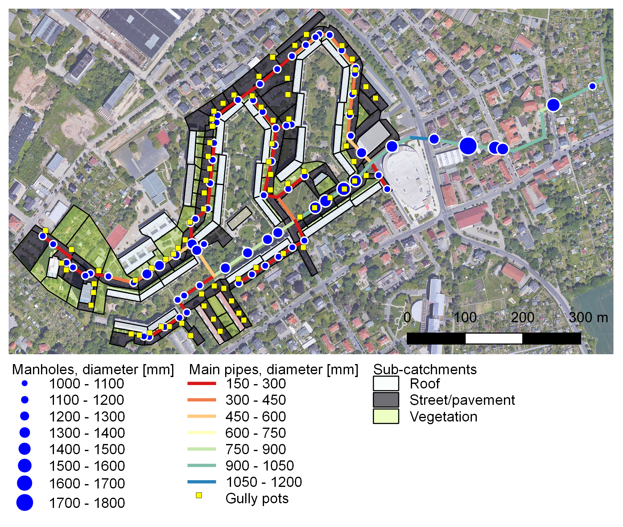
The paper is divided into five parts. The introduction to the general topic is followed by an overview of the study site and data used (Section 2.1) and model build-up (Section 2.2). The methodology part presents a model calibration procedure (Section 2.3), explains how the overloading of the drainage system is implemented in the SWMM (Section 2.4), and describes the statistical methods for the post-processing of the results (Section 2.5). The results part contains the model set-up and calibration performance (Section 3.1), the outcome of the model runs with different scenarios (Section 3.2), the statistical analysis of the results with pairwise correlations (Section 3.3) and MLR (Section 3.4), and a discussion of the influence of precipitation resolution (Section 3.5). Finally, conclusions are drawn and outlooks are discussed in Section 4.

2. Data and Methods

This section describes the general methods and tools used to complete the previously listed tasks as well as a description of the study site and data specification. This includes data collection and processing, the set-up and calibration of the SWMM, and the statistical analysis of the results.
Figure 1 presents the applied workflow. It starts with the collection and processing of terrain and land cover data, all possible information on the sewer system, and climate data. Then, the model is set-up in the SWMM and calibrated using observed time series and design/observed heavy precipitation events used for the model forcing. Finally, the output data are statistically analyzed with a focus on the SWSS overloading.

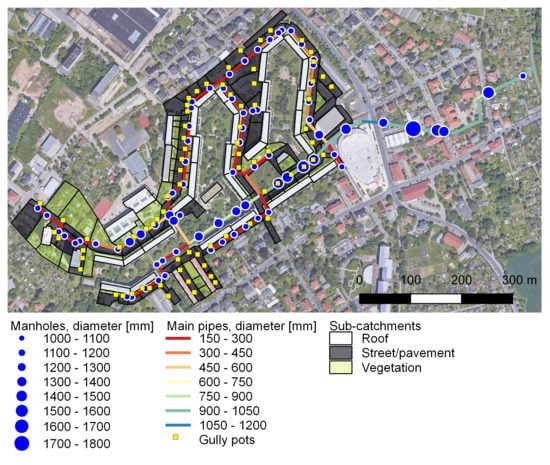
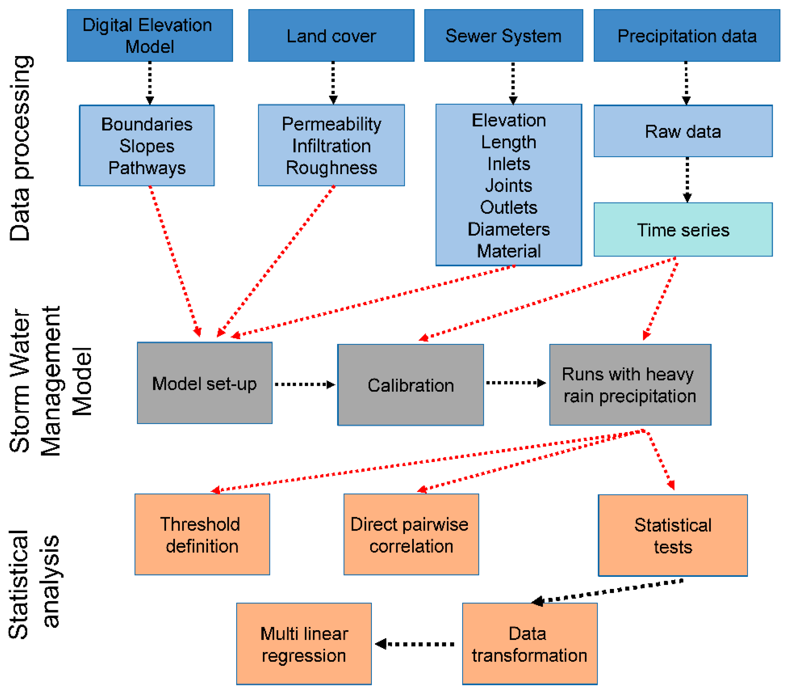
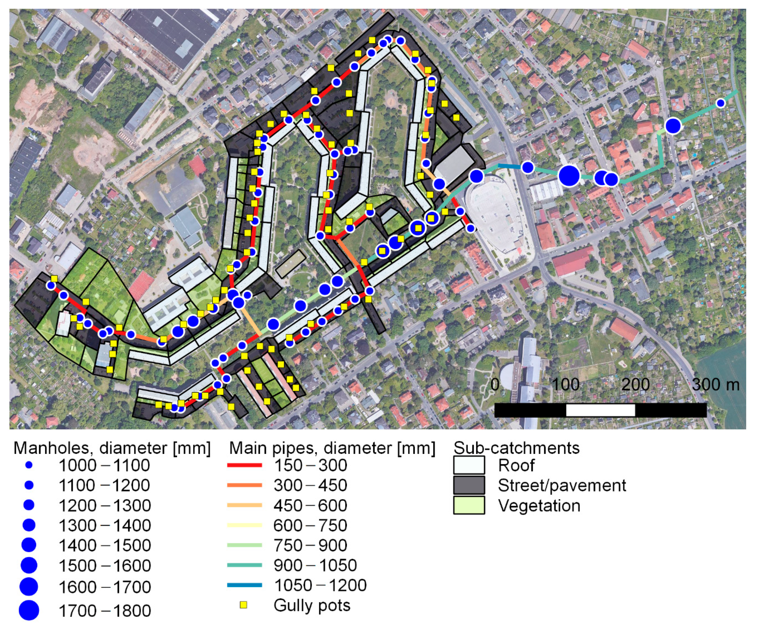
2.1. Study Area and Required Initial Data

The study site is located in the south-eastern part of Dresden, Germany (51.00277°, 13.8374°, Figure 2) and has a drainage area of 0.12 km2. The land cover shows a typical urban configuration with approximately 50% of impervious areas: buildings (block living, schools, and grocery stores), pavements, parking lots, and green (mainly grass) areas. The topography consists of mostly flat slopes with a general drainage direction to the north-east. In this specific area, a separated urban drainage system was installed initially, meaning that stormwater and sewage flow in parallel, but separated, pipes. The SWSS is formed of approximately 2.7 km of pipes, connected by 91 manholes, receiving water through 69 gully pots and discharges water in the local creek, which then flows out to the Elbe.
Table 1 presents the required data for the modeling in the SWMM and the used sources.
The specification of an SWSS should include at least a detailed geometry of the pipe system and connections, such as elevations, lengths, diameters, shapes, the materials of pipe sections, and junctions, which are usually obtained from construction/monitoring documentation or field surveys. For the study, SWSS data were produced and provided by the Urban Water Management Department of TU Dresden; however, a small field survey was additionally conducted to correct the positions of some manholes and locate all the gully-pots, since they were not presented on the schemes.
Detailed information on the catchment is required to set-up the general boundaries of the SWSS, delineate sub-catchments, calculate drainage areas and terrain slopes, assign flow pathways to SWSS inlets, and determine the main catchment parameters (roughness, width, permeability, infiltration, depression storages, etc.). These data can be retrieved from satellite images, remote sensing elevation data or topographic maps, and field surveys, and some parameters can be found in textbooks. For the present study, a digital terrain model (DTM) of one-meter resolution (produced and provided by the TU Dresden), OpenLayer QGIS plugin [30] (which incorporates Open Street Maps and satellite images (Bing and Google)), and results of a small field survey were used.
Climate data include those of precipitation and temperature. While the first are the critical data for the model forcing, the second are additional ones to estimate daily evaporation (Hargreaves’ method). The main intention was to simulate heavy rain precipitation events. Therefore, assuming negligible evapotranspiration fluxes during extreme rain events, other climatic data were not considered. Precipitation data were obtained from the nearest meteorological stations (Figure 2) from the database of Deutscher Wetterdienst (DWD, German Meteorological Service) [28]. Furthermore, design precipitation events with various characteristics were constructed from the KOSTRA-DWD-2010R (Koordinierte Starkniederschlagsregionalisierung und -auswertung des DWD (coordinated heavy precipitation regionalization and evaluation)) dataset [29]. Distributed via gridded (resolution of approximately 67 km2) rasters for the whole of Germany, this dataset consists of pre-calculated design heavy precipitation via block-rain (rectangular hyetograph). The user can choose specific values of precipitation sums (in mm) and intensities (l s−1ha−1) depending on different event durations (5 min to 72 h) and RPs (1–100 years).

2.2. Model Build-Up

The initial SWSS data on pipes, manholes, and outlets were checked for apparent errors—i.e., misconnections, typos in diameters, and manhole position errors—and all the gully-pots found within the field survey were added (with an average depth of 1 m) and routed to the associated manholes. The fixed parameters for inlets and junctions include shape, elevation, and depth; those for pipes include shape, length, and diameter. Since there is no option in the SWMM to select variable node diameter, the nodal surface area of 0.44 m2 was established as a weighted mean of the standard manhole and gully-pot chamber diameters installed in the studied SWSS. The application of a weighted rather than simple mean is explained by the different numbers of gully-pots (69) and manholes (91); thus, taking a simple mean value will give a lower value for the effective diameter. It is important to estimate this parameter with proper justification, since it has a direct effect on the inundation characteristics because it defines the nodal volume, which acts as a buffer before SWSS overloads.
Afterward, the sub-catchments of the three main presented land classes (streets/pavements, roofs, and vegetation) were delineated according to the DTM and satellite images and assigned to the SWSS inlets. The fixed parameters for the sub-catchments included area, mean width, terrain slope, imperviousness (80–100% for streets/pavements, 100% for roofs, 20% for vegetation), and infiltration parameters (capillary suction head: 100 mm; saturated conductivity: 10.9 mm h−1; the difference between porosity and initial moisture content: 10%) for the mean soil type in the area (sandy loam) used in Green–Ampt method [31]. The area-related characteristics were calculated in QGIS [32] (“Field calculator” and “Terrain analysis” tools), the permeability was assigned according to satellite images [25,26], and the field survey, and the soil hydraulic properties were taken from the SWMM recommendations [33].
The general SWMM parameters (different from defaults) included rainfall/runoff and flow routing modules, the dynamic wave routing model, a routing step of 1 sec, and a head convergence tolerance of 1 mm.
The SWSS and catchments (with necessary characteristics and parameters) were prepared with QGIS 3.4.15 [32]. The final transfer from “shp” files to “inp” (SWMM data format) was done using inpPINS [34]. An overview of the model is presented in Figure 3.

2.3. Model Calibration

Two major approaches are commonly used in the calibration of the hydrological model—continuous and (multi-)event matching. Since the study investigates modeling storm events and the overloading of the SWSS, a calibration with short heavy rain events instead of long time-series with dry weather or regular stormwater flow is more likely to provide more accurate results. This multi-event approach is quite popular in practice for the same kind of studies and used by various researchers using different hydrological and hydraulic models [35,36,37,38]. It was already successfully applied in the nearby sub-catchment for studies of low impact development practices [39].
Depending on the availability of observation data, the model can be calibrated using various techniques and with different performance indicators. In general, there are many parameters available for validation in the SWMM: sub-catchment runoff, node/pipe water depth, pipe/node inlet/outlet discharge, and node flooding.
Conventionally, urban sewer system models are calibrated using the outlet pipe discharge (i.e., outfall to a local open channel or inlet to a wastewater treatment plant), hence by hydrograph comparison. Thus, to evaluate the goodness of the model results, several well-known performance criteria can be used (Table 2): Nash–Sutcliffe Efficiency [40], Kling–Gupta Efficiency [41], and peak and volume errors.
The calibration procedure could be performed in automatic (by the definition of the cost function and iterations using preset boundary values for the chosen calibration parameters) or manual (changing parameters “by hand”) mode. The selected mode depends on the model complexity and the number of changing parameters. For the particular case-study, manual mode was chosen due to the event-based calibration and the use of only a few parameters (pipe and surface roughness, contribution areas, and depression storages).

2.4. Overloading of the Stormwater Sewage System in SWMM

In the present study, an urban flood in an SWSS is considered as a process of drainage system overloading caused by heavy rain, which leads to the flooding of the surface. In the SWMM, this phenomenon is modeled as follows. Each non-outfall node is assigned a maximum allowable pressure head Hmax. It consists of a maximum free water surface elevation (i.e., manhole depth) plus an optional “surcharge” depth that allows for an additional pressure head (i.e., if a manhole has a solid cover without openings). Typically, when the new head Hnew at a node is computed by the iterative solution process, and it exceeds Hmax, it is set equal to Hmax, and the node becomes flooded. Then, the overflow rate Qovfl is calculated as an average net flow rate (inflow−outflow) of the node over the current time step [27].
Therefore, the flooding parameters are available in the model summary for each flooding node: total flooded time, maximum flooding discharge, time of maximum flooding, and total flooding volume.
A critical remark to add is that once flooding occurs, afterward, this flooding volume is then lost from the system, as the SWMM does not allow overloading water routing.

2.5. Statistical Post-Processing of the Results

Two statistical approaches were used to study the relationship between precipitation and the SWSS overloading parameters: pairwise correlation and MLR.
The classical Pearson correlation test used as the first approach is a measure of the linear correlation between two variables.
MLR is a relatively powerful yet simple tool to increase the correlation coefficient of the dependent variable using non-clear individual relationships with predictors. The general formula for the MLR function is as follows:
y = a + i = 1 i = n b i · x i
where y is the dependent variable, x i is the predictor, a is the intercept, b i is the slope, and n is the number of predictors.
This approach was used to find a better relationship between precipitation and the SWSS overloading parameters. However, to fit the MLR function properly, the data and the obtained regression should fit the relatively strict statistical assumptions [42] listed in Table 3.
Conventional statistical tests are used to test for the normality of the data (Shapiro–Wilk [43]), the autocorrelation of residuals (Durbin–Watson [44]), and the homoscedasticity of the variance (Breusch–Pegan [45]). The general interpretation of the tests comes down to a comparison of the test statistics’ p-values to a conventional threshold value of 0.05 [46] to decide on the rejection (p < 0.05) or non-rejection (p > 0.05) of the test null hypothesis. The following null hypotheses denote the chosen tests (Shapiro–Wilk, Durbin–Watson, and Breusch–Pegan, respectively): a sample comes from a normally distributed population; there is no autocorrelation (at a lag of 1) in the residuals (prediction errors) according to a regression analysis; the variance of the errors according to a linear model is homoscedastic.
Additionally, data transformation methods were used to convert non-normally distributed data to an approximately normal distribution. The simple reason for this is that in fact, after transformation, one is able to “recycle” the knowledge about the analysis of the normally distributed data, so that one can apply standard analysis methods. An outstandingly important class of transformations is powers and logarithms. The so-called Box-Cox transformation is applied to determine an optimal transformation for this class [47]. The original formula looks like this:
x i = { x i λ 1 λ · G M ( x ) λ 1     i f   λ 0   G M ( x ) · ln ( x i )   i f   λ = 0  
where: G M ( x ) —the geometric mean of the sample and λ —maximum of the log-likelihood function (assuming the transformed observations come from a normal distribution with mean μ and standard deviation σ, the log-likelihood function looks as follows l o g [ L ( λ , μ , σ ) ] ). In this study, a simplified version of Box-Cox transformation was used, with the formula x i = x i λ and λ rounded to closest value with a 0.5 step (which, however, still remained within the 95% confidence interval).
Statistical analysis was conducted within the R environment [48] using standard and the following custom libraries: “lmtest” [49] and “MASS” [50].

3. Results and Discussion

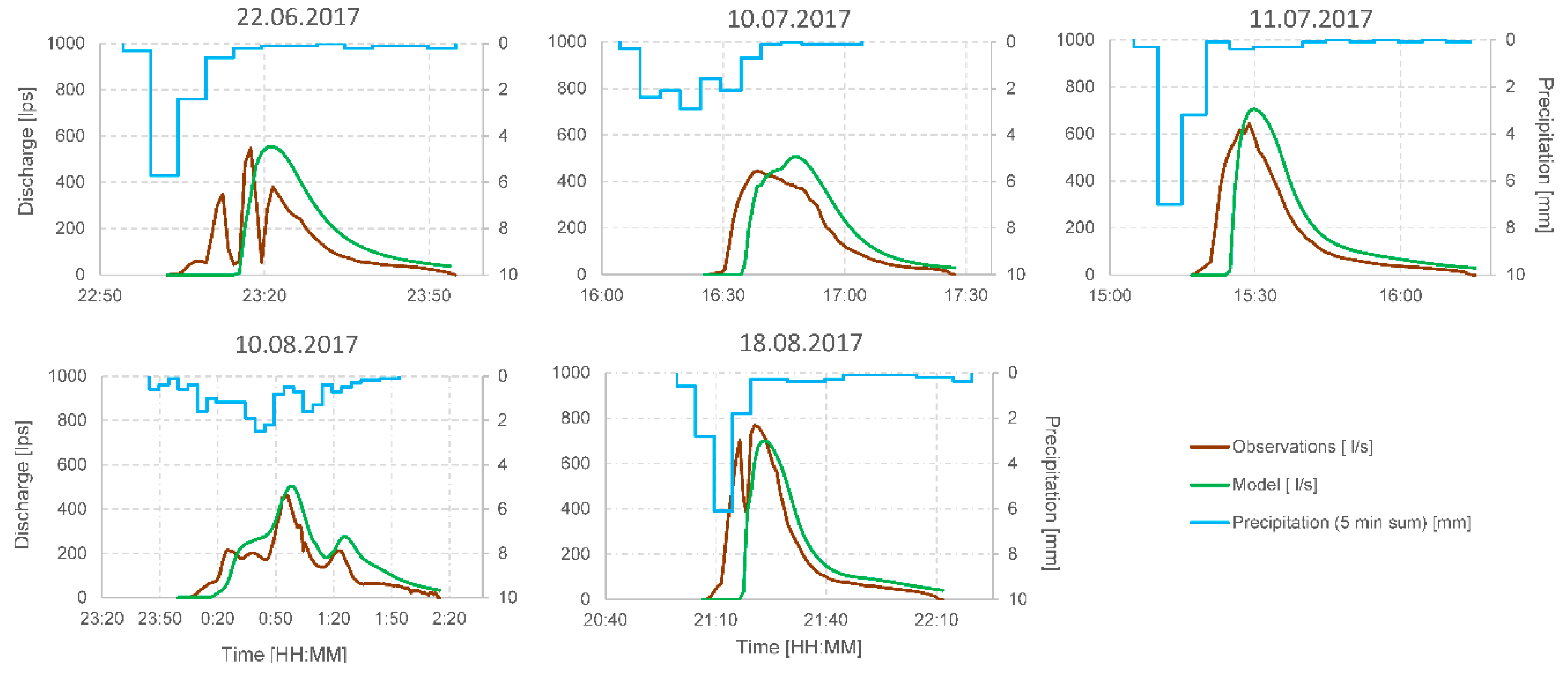
3.1. Model Calibration

For the calibration of the model, almost two years (01.2017–10.2018) of irregular discharge measurements in the outflow to Lockwitzbach creek were available at a 1 min resolution (taken and provided by the Urban Water Management Department of TU Dresden). For the model forcing, meteorological input data of the closest station (Lockwitz, 1.6 km from the catchment) with a 5 min resolution were used. As the goal was to calibrate the model using the event-based principle specifically for high-flow conditions, available discharge time series were screened, and five flood events were extracted. To gain more accurate calibration parameters and because of the already too-small sample size, the authors decided to sacrifice the normal procedure of splitting data into calibration-validation sets and instead used all the events for calibration purposes. This trade-off indeed weakens the reliability calibration procedure and needs to be elaborated in possible future studies when longer observation time series will be available.
The calibration was performed manually, and the chosen fitting criteria were the following: peak discharge, time to peak, and total volume. The first two were met by adjusting the roughness of the conduits (0.0155 m1/3s−1, accounting for the pipe material and conduits’ current conditions) and catchments (0.016 m1/3s−1 for impervious and 0.03 m1/3s−1 for the pervious terrain). The recommended range of Manning’s coefficients for steel and plastic pipes (whose mixture forms the studied SWSS) is 0.009–0.19 m1/3s−1 [27,51]. The ranges of the coefficients for the surface roughness were taken from [52]: 0.01–0.023 for impervious (smooth and rough asphalt, tar, and concrete) and 0.017–0.06 m1/3s−1 (smooth and rough packed soil, gravel, grass, and residential land use). Additionally, catchment depression storage parameters were used in the calibration: percentage of impervious area with no depression storage (50%) and depth of depression storage on pervious/impervious area (for vegetation: 5/1 mm; for streets: 5/2.6 mm; and 1.27 mm for roofs). Various estimations and formulas [33] suggest the following ranges for depression storage: in general, values of 0.1–11 mm are mentioned; specifically, with empirical formulas, 0.1–2.8 mm is suggested, and with case study estimations, –1.2 to 2.5 or 5 to 11 mm for impervious or pervious areas are suggested, respectively. Hence, parameters exhibit strong variation from study to study, and extensive preliminary work to obtain accurate estimates or to fit them within the exact the ranges of empirical formula outcomes or other researcher’s values is unnecessary. Moreover, this parameter was stated as being sensible only for low-depth short storms [33]. Fitting the flood volume could be adjusted by rearranging the catchment boundaries, adding missing or deleting areas that are clearly not contributing to SWSS runoff. This can be achieved with the help of satellite images and consideration of the impressions from an on-site survey. In the study case, mainly pervious areas and roofs were deleted. Figure 4 shows the comparison of the measurements and the calibrated model output for the five events and the corresponding precipitation, and Table 4 presents the results for the performance criteria.
A relatively high agreement was achieved for four out of five events. The NSE values for these four events are around 0.5, and the KGE values, around 0.7. Regarding the lower performance of the event dating 22.06.2017, the issue with the low NSE values could be explained by the general problem of time shift for all the events in the range of 3–10 min. Several attempts to adjust timing were conducted, and the only case where the time-shift of the uprising limb was matched related to lowering the conduit roughness to 0.008–0.009 m1/3s−1. However, firstly, these values do not look realistic for a relatively old pipe system (besides enormous velocities of 2–4 ms−1), and secondly, they resulted in the shortening of the flood duration almost twice while sharply increasing the maximum flow rate. The most probable background of this effect is the travel time of the rain cell, as there is a distance of 1.6 km between the study area and the meteorological station (resulting in propagation velocities of 3–10 ms−1, which are reasonable, i.e., for convective cells [53,54]). Thus, the issue was considered as non-crucial for the study, since in this case, it will not affect the characteristics of SWSS overloading. That is why it is important to have a look at the KGE values (whose component decomposition will give a low correlation value but high bias and variability ratio agreement), which are all higher than −0.41 (benchmark of mean flow performance [55]).
The higher and positive volume errors (12–31%) gained for four out of the five events are potentially a bigger problem for the study set-up. However, as can be seen from the graphs, in most cases, these volumetric errors are the sum-up result of too long tails of modeled hydrographs, while the observed ones are much shorter. Nevertheless, as the main intention of the study was inundation research, the main interest lies in the upper part of hydrographs, where a better agreement was achieved. Generally speaking, these deviations could probably be explained by the different resolutions of the discharge and precipitation measurements (i.e., for 22.06.2017 and 18.07.2017, three and two clear peak inflows are observed, respectively, while only one is found in the precipitation measurements). The relative peak errors are much smaller (−9 ± 14%) and potentially result from the generalization of the initial model conditions (as the event-based calibration strategy does not normally imply a warm-up period like in conventional continuous calibration) or simplifications of the surface flow routing in the SWMM. The apparent overestimations and underestimations of the peak discharge and total volume are again the probable results of the different resolutions and heterogeneity of the rain cell, which is a known issue for SWSS modeling [56].

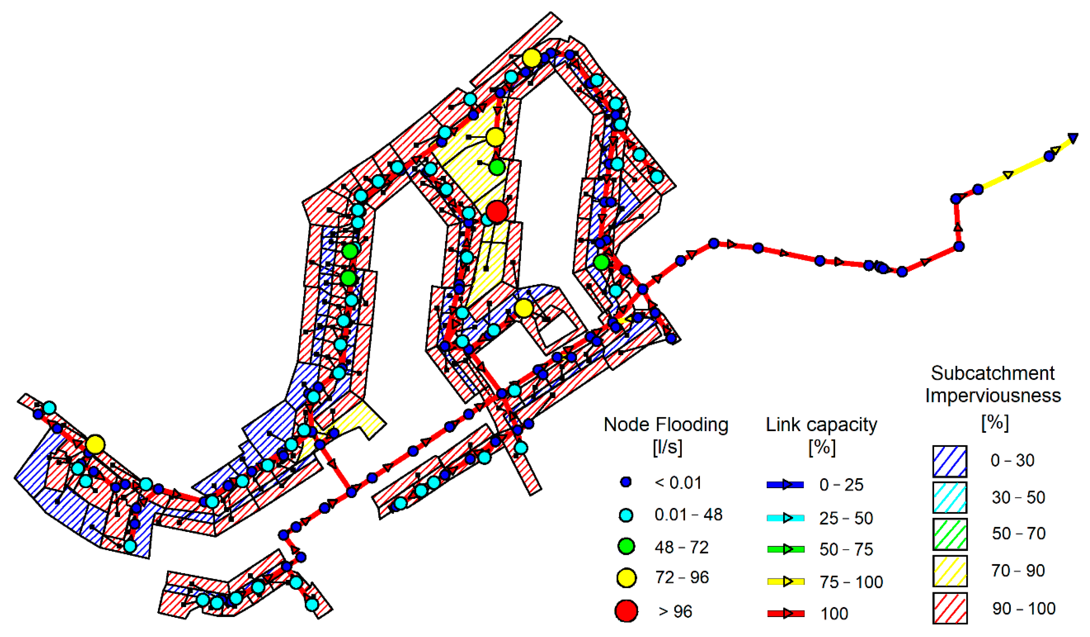
3.2. The Model Runs with Various Heavy Precipitation Scenarios

Data from the three nearest meteorological stations (Figure 1) were screened within the available time-period of 1998–2018 [28] to extract 35 heavily observed precipitation events, with a precipitation measurement interval of 1 min (the data from the nearest Lockwitz station are available only with a 5 min resolution and much shorter time period). To get an insight into the sensitivity of the model to different input data types, KOSTRA-DWD-2010R (see Section 2.1) was used and the following design rain events were extracted: RPs of 2, 20, and 100 years and durations of 5, 10, 120, and 2880 years. For each of the rain events, the following characteristics were derived: duration, sum, maximum intensity (Imax), mean intensity (Imean = sum/duration), form (K1 = maximum intensity/sum), skewness (K2 = time to peak/duration), and flatness (K3 = maximum intensity/mean intensity). K1, K2, and K3 were added to account for a pluviograph shape: K1 indicates the steepness of the event (values close to 1 indicate a very steep event, as the maximum intensity and sum are equally big), K2 marks whether the peak comes at the beginning or the end of the rain event, and K3 describes how pronounced the peak of the rain is compared to the mean intensity of the event. Table 5 shows a summary of the scenarios, and a full list is presented in Appendix A. A subset of the observed rain events was made to cover a relatively wide range of the possible combinations of precipitation characteristics but, in general, starting from short light rains, which are unable to overload an SWSS (but are necessary to detect the overloading threshold), continuing with long/short events of moderate intensity, and, finally, finishing with long/short heavy precipitation with RPs of 20–100 years.
A summary of the SWMM simulation results is presented in Table 6, and a full list with all the model outputs is presented in Appendix B. In case flooding occurred, the maximum flooding time (among all flooded nodes), discharge at the most pronounced junction, and total flooding volume in the whole SWSS were reported. If no flooding was observed, the relative node depth at the most loaded junction is documented (calculated as the ratio between the maximal water depth and total manhole depth).
Figure 5 illustrates an event triggered by a 100-year RP heavy rain with the biggest total flooding volume at the moment of maximum loading and, consequently, flooding of the system. The flooding occurs at 58 different nodes (five manholes, 53 gully pots) with varying intensities. Additionally, almost all of the conduits are filled to their maximum capacity.

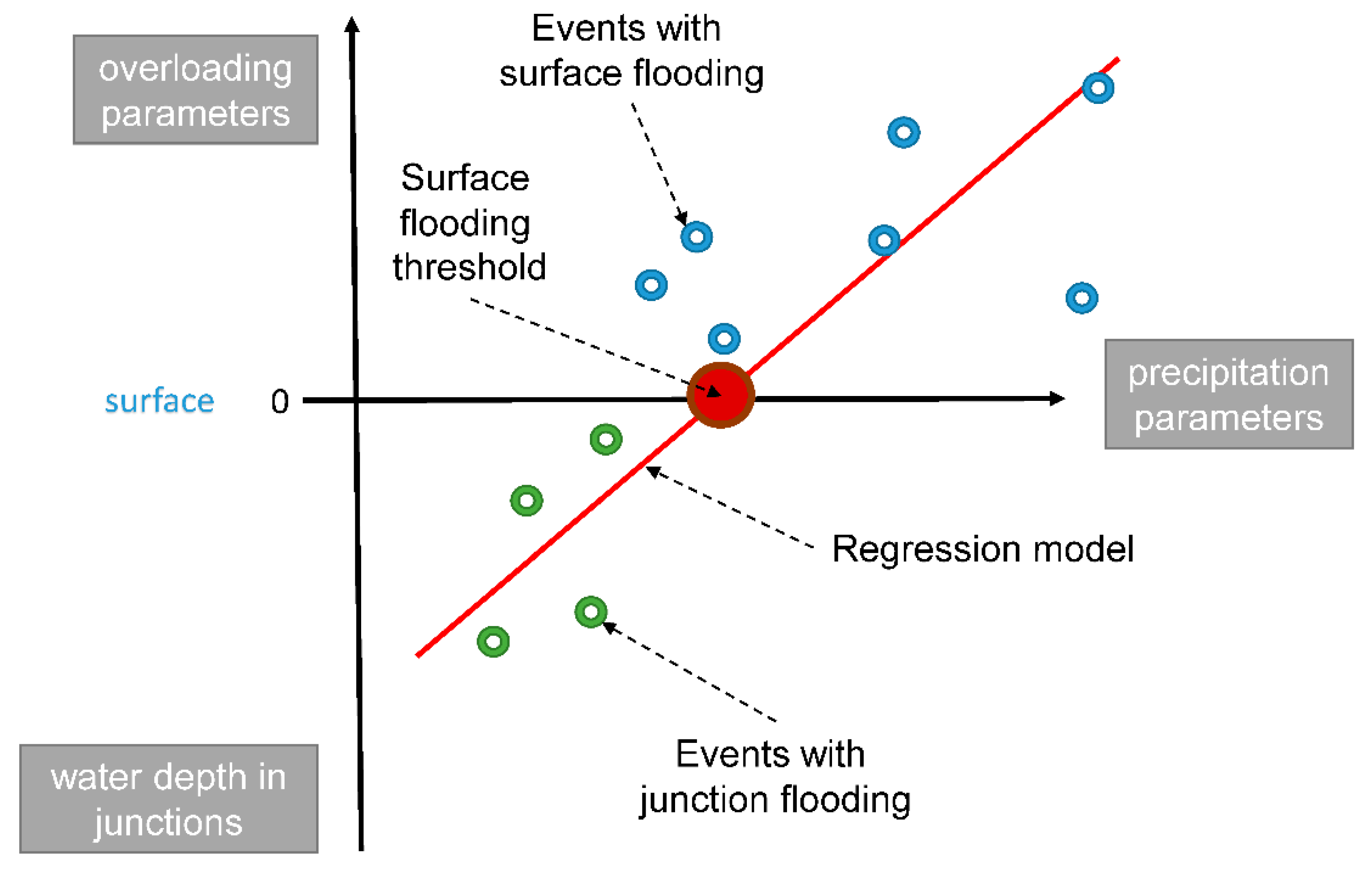
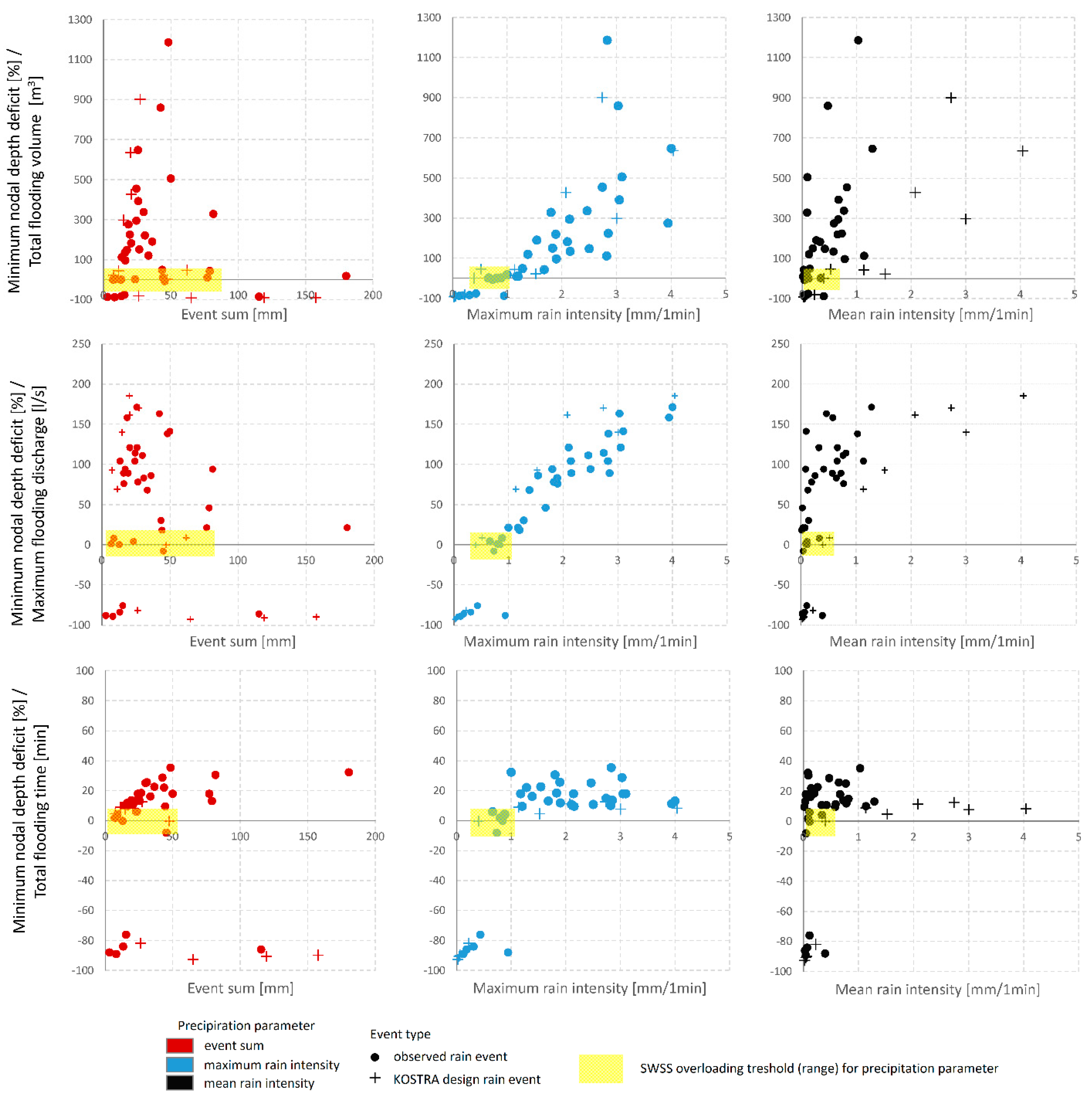
3.3. Detection of “System Overloading” Precipitation Threshold

To find the precipitation threshold for SWSS overloading, a graphical solution is proposed. Using flooding values obtained from the SWMM simulations (i.e., flooding volume) and parameters of rain events (i.e., maximum intensity), the upper part of the graph (Figure 6) is defined. With the intercept of the X- and Y-axis representing the virtual terrain surface of the system (the elevation of the manhole top), the lower part of the graph defines non-surface-flooding conditions by the maximum water depth in the node (or relative nodal loading—for better scaling) during a rain event. Hence, the intercept will give the surface flooding threshold of the SWSS for a specific precipitation parameter.
Table 7 shows the Pearson’s correlations calculated for all scenarios and excluding design events. Among all the precipitation parameters tested, a few of them (duration, sum, mean and max intensity, and K1) depicted significant (p < 0.05) negative and positive correlations with inundation parameters. In summary, it could be stated that, in general, rain events with a shorter duration, higher maximum intensity, and total sum will cause higher SWSS flooding time, discharge and total volume, which is in agreement with the findings of other studies [15,16] (partly, since no studies were found to cover correlation with all the used precipitation characteristics). An exclusion of KOSTRA design rain leads to an improvement of the correlation, while block-typed and natural rain events lead to a different response of the SWSS. Since civil engineers usually use design rainfall for planning drainage systems and scientists stick to real observation data, there is no right answer as to which data type is better. However, the authors want to highlight the message that due to the significantly different relationship between the overloading and precipitation parameters, design and observed rain events should not be mixed together, to obtain better results.
Picking up the three most promising precipitation parameters (sum, mean, and max intensity), an attempt to find an SWSS-overloading threshold with a graphical approach was conducted (Figure 7). The results indicate a not very good relationship, since even if a linear function can be derived for the upper part of the graph, most often, the points from the bottom (the maximum node loading) have different relationships or/and are indistinct. Therefore, the possible ranges of the interception with the 0-ordinate axis representing the starting of SWSS flooding are relatively big. Nevertheless, for the maximum intensity, it is possible to detect the upper and lower values of the threshold for each flooding parameter (0.2 and 1 mm/min, respectively) and for the event sum and the mean intensity—at least at the upper boundary (60–90 mm and 0.6 mm/min, respectively).

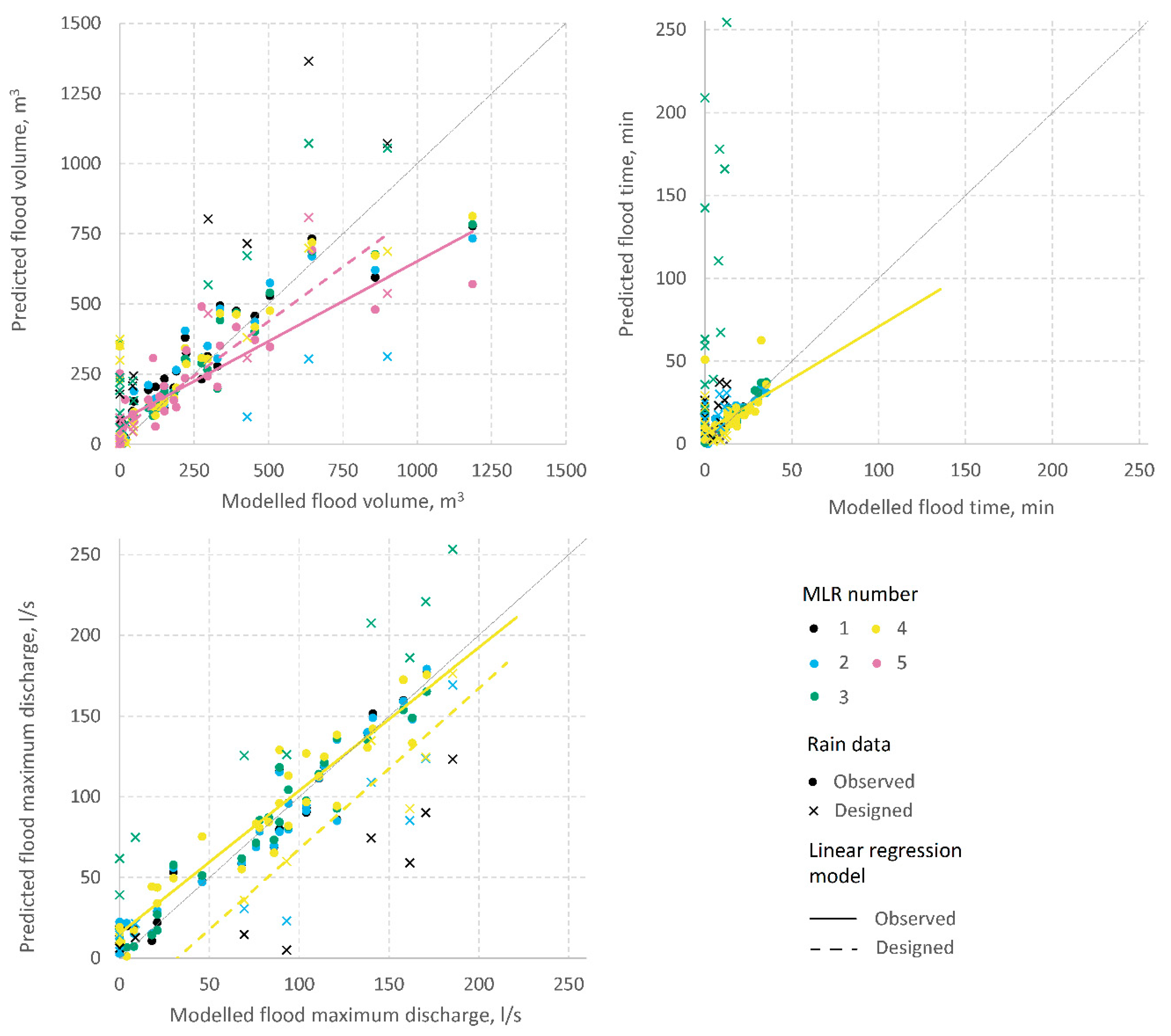
3.4. Prediction of Overloading Parameters with Multi-Linear Regression

To increase the predictability of the flooding occurrence and its parameters in particular, a second approach was followed. The MLR was fitted to various combinations of the precipitation parameters to determine whether this method improved the correlation compared to the pairwise approach. Here, observed and designed rain events were not separated and acted as one dataset. The adjusted coefficient of determination (squared correlation coefficient corrected by the number of predictors) was used as an MLR selection performance measure. The following models were tested: one/two with original data (all predictors and reduced number if the fit was better) and two/three with transformed data (all predictors, best predictors with which MLR fits all statistical assumptions, and best predictors without assumption fitting). The reduction of predictors was based on the pairwise correlation analysis and the significance of a specific predictor’s coefficient in the summary print of MLR.
At first, the data were tested against the MLR assumptions mentioned in Section 2.5. Approximate linearity could be confirmed with simple scatter plots (i.e., for the exemplary data in Figure 7). The independency of certain predictors within a certain pool is defined by parameters such as duration, sum, and intensity (which are the only ones that are strictly independent); however, a pair like sum and K3 are also valid. The results of the normality test and histograms for the direct model output showed a skewness of the data distribution. Thus, a transformation was necessary. Table 8 shows the result of the Shapiro–Wilk test before and after Box-Cox transformation; additionally, the transformation parameters are depicted. It could be stated that for all the parameters (except duration), logarithmic and power (square root) transformation worked, and approximate normality was achieved. Other assumptions (normality and the absence of the autocorrelation of the model residuals as well as the homoscedasticity of the variance) had already been tested after the model fitting employing the Shapiro–Wilk, Durbin–Watson, and Breusch–Pagan tests and MLR diagnostic plots. A summary of the MLR model fit results and list of the used predictors are shown in Table 9, and the adjusted coefficients of determination and p-values of the applied tests are presented in Appendix C. While there were no problems with the residual’s autocorrelation and homoscedasticity for any of the models, non-transformed data exhibited problems with normality. Finally, only the model with independent predictors and transformed data fitted all the assumptions. Overall, the coefficients of determination varied from 0.70 to 0.92, with better performance for the maximum overloading discharge and slightly worse performance for the total overloading volume.
A graphical representation of the performance for all the tested MLRs and all three overloading parameters is presented with the scatter plots of those modeled versus those predicted with MLR values (Figure 8). It can be observed that none of the derived functions delivers a perfect match. In fact, there is a tendency to detect flooding when it was not found in the SWMM output and, vice versa, to underestimate the flooding parameters at high ranges. As expected from Table 9, the maximum nodal flow rate has much better predictability, while for the flooding time, it seems to be very tricky to achieve good results. Finally, it is clear that the obtained MLR works much better for the observed rather than for the designed rain events, especially at high ranges.
Transforming the coefficient of determination to Pearson’s correlation, one can finally determine whether MLR outperformed the pairwise correlation. Using only the MLRs that fit all the statistical assumptions, it can be stated that MLR could considerably improve the prediction of the flooding time and volume (Table 10) by approximately 20–40%.

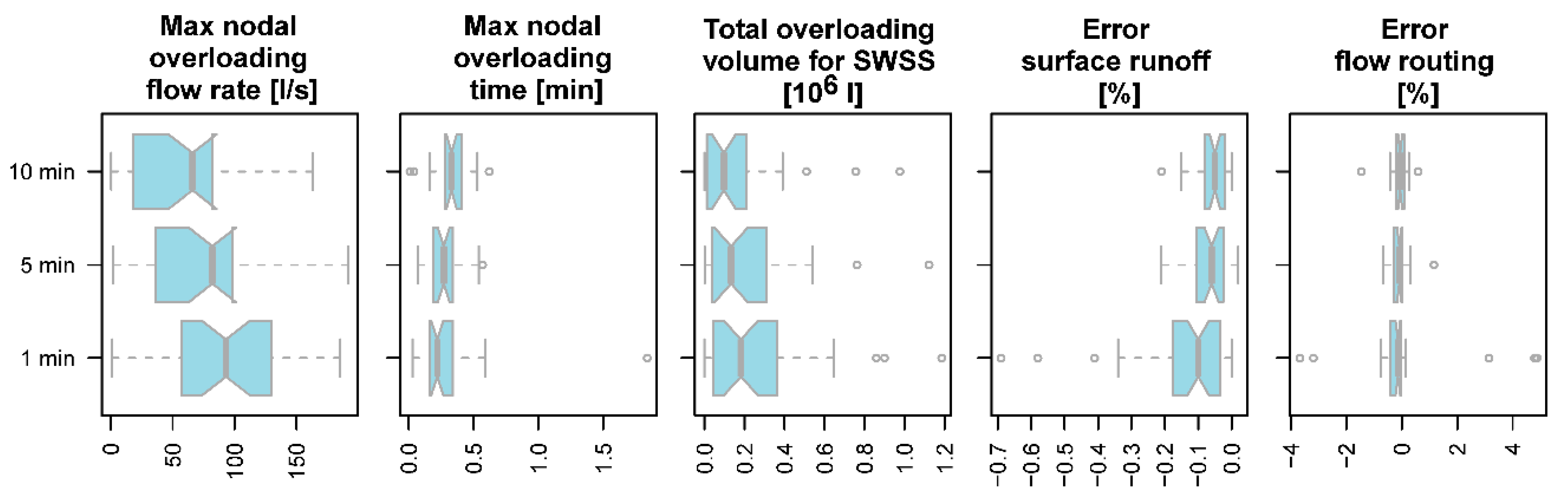
3.5. Influence of the Precipitation Resolution

To test the sensitivity of the model to overload depending on the input data quality, all the scenarios with observed precipitation were rerun with the up-scaled resolution of 5 and 10 minutes. The results indicate that an increase in the precipitation aggregation period yielded a decrease in the overloading volume and maximum flow rate and an increase in the maximum flooding time (Figure 9). However, ANOVA tests showed that the changes are significant (p < 0.0.5) only for the maximum flow rate. Additionally, simulation errors were compared: the surface runoff errors decreased significantly with an increase in resolution, while the flow routing errors remained almost at the same level. Overall, this means that even in the absence of highly resolved precipitation measurements, the modeling of SWSS overloading could give good results. These results agree with other studies, which show that precipitation aggregations do not lead to the same noticeable degree of changes in SWSS flow [57].

4. Conclusions and Outlook

The presented study gives novel insights into the behavior of stormwater sewage systems in the urban areas concerning their overloading due to heavy rain events, using a numerical modeling approach and statistical post-processing of the results. Using a case study of a small catchment in Germany, an SWMM model was set up and calibrated. Several scenarios with observed and designed precipitation events were tested to study the correlation between rain characteristics and overloading to detect the flooding of the system and predict its parameters. In our opinion, the goals of this study were reached, and the case study showed that the methods are applicable and most possibly transferable. The following conclusions can be drawn:
  • The prediction of SWSS overloading using rain forecasts with precipitation characteristics and a proposed graphical approach is, in general, possible. However, the relationship between the upper (surface flooding) and the lower (nodal flooding) parts is quite fuzzy for some precipitation parameters. For the studied SWSS, surface flooding most probably will start after rain with around 1/0.6 mm min−1 of maximum/mean intensity and a total event sum of more than 60 mm.
  • The total overloading volume and maximum overloading flow rate showed a higher Pearson’s correlation with the maximum rain intensity (R = 0.67 and R = 0.93, respectively), and for the maximum flooding time, the total rain event sum worked better (R = 0.59).
  • MLR with the precipitation characteristics can significantly improve the predictability of the SWSS overloading parameters (with an increase in the Pearson’s correlation coefficient up to 50%). This, however, could require additional data manipulations.
  • Observed and designed rain events behave differently in terms of SWSS overloading; thus, the analysis and results should be treated separately.
  • The use of the coarser precipitation resolution leads to a decrease in the SWSS overloading volume and maximum flow and increase in the flooding time (relative changes in median values by approximately 20–30%).
Besides scientific value, the suggested methods can potentially be applied to improve sewer system design for extreme scenarios or to establish simple early warning systems for SWSS inundation based on rain forecasts (without comprehensive operational modeling frameworks) and thus provide a quick response to support preparations for flooding and the mitigation of its consequences.
Finally, the authors would like to highlight possible future steps for extending the presented study in the field of extreme precipitation and the prediction of SWSS overloading:
  • Testing the approach on different catchments, and the extension of the event sample size to obtain more robust statistics;
  • In-depth research into SWMM event-based calibration for heavy precipitation events;
  • Validating the approach with observations;
  • Incorporating models capable of the surface routing of overloaded water.

Author Contributions

Conceptualization I.V., F.S., J.B., and F.A.J.; resources (data provision) F.A.J.; formal analysis, methodology, and investigation, I.V., F.S., and J.B.; writing—original draft and visualization, I.V.; review, F.A.J., F.S., J.B., and P.K.; supervision, F.A.J. All authors have read and agreed to the published version of the manuscript.

Funding

Open Access Funding by the Publication Fund of the TU Dresden.

Conflicts of Interest

The authors declare that they have no conflict of interest.

Data Availability

The calibrated model, raw data on the SWSS, discharge measurements, DTM, and prepared heavy precipitation dataset used in the presented study can be provided upon request. The raw climatological data can be obtained from the DWD server [28]. The rasters with design heavy precipitation can be obtained from the KOSTRA-DWD-2010R server [29].

Appendix A

Table A1. Observed and designed rain events.
StationDuration (min)Sum (mm)Max Intensity 10 min (mm/min)Max Intensity 5 min (mm/min)Max Intensity 1 min (mm/min)Mean Intensity (mm/min)K1K2K3
1Hosterwitz914219.5010.113.030.470.070.250.15
2Hosterwitz1413610.056.701.540.260.040.340.17
3Hosterwitz44611151.240.710.180.030.000.090.14
4Hosterwitz272011.2710.242.850.720.150.220.25
5Hosterwitz321914.5211.153.940.580.210.720.15
6Strehlen483111.366.991.890.640.060.480.34
7Strehlen314447.064.661.280.140.030.700.11
8Strehlen12148.305.332.821.140.210.830.40
9Strehlen372413.028.462.140.660.090.680.31
10Strehlen474815.8011.672.831.030.060.150.36
11Strehlen211610.475.781.900.780.120.520.41
12Strehlen1998776.103.971.170.040.020.090.03
13Strehlen1024453.052.050.730.040.020.630.06
14Strehlen281613.057.382.150.570.130.180.27
15Klotzsche9218212.808.401.800.090.020.390.05
16Klotzsche23301807.404.301.000.080.010.240.08
17Klotzsche2826445.304.001.200.020.030.640.01
18Klotzsche5255018.9010.203.100.100.060.010.03
19Klotzsche421711.009.402.500.410.140.400.17
20Klotzsche632110.408.602.100.330.100.170.16
21Klotzsche202621.6011.104.001.280.160.300.32
22Klotzsche1372711.916.661.830.190.070.080.11
23Klotzsche393012.857.992.460.770.080.310.31
24Klotzsche302512.3410.472.740.820.110.300.30
25Klotzsche2673312.016.151.380.130.040.060.09
26Klotzsche2674796.925.431.680.030.020.080.02
27Klotzsche392615.639.453.050.670.120.210.22
28Hosterwitz8274.843.120.800.090.110.170.11
29Strehlen204132.171.120.310.070.020.190.21
30Strehlen213234.262.670.660.110.030.510.17
31Hosterwitz21280.670.410.120.040.010.550.32
32Hosterwitz143163.701.940.430.110.030.450.25
33Hosterwitz833.142.540.940.390.300.380.42
34Strehlen2794.722.830.880.340.100.700.38
35Klotzsche117133.572.370.840.110.060.640.13
36Kostra RP25815.207.601.521.520.20--
37Kostra RP2051530.0015.003.003.000.20--
38Kostra RP10052040.4020.204.044.040.20--
39Kostra RP2101111.305.651.131.130.10--
40Kostra RP20102120.7010.352.072.070.10--
41Kostra RP100102727.3013.652.732.730.10--
42Kostra RP2120262.191.100.220.220.008--
43Kostra RP20120473.951.980.400.400.008--
44Kostra RP100120625.182.590.520.520.008--
45Kostra RP22880650.230.110.020.020.0003--
46Kostra RP2028801200.410.210.040.040.0003--
47Kostra RP10028801580.550.270.050.050.0003--

Appendix B

Table A2. Results of the model run with 1 min resolution precipitation input.
Max Nodal Overloading Time (min)Max Nodal Overloading Flow Rate (l/s)Total Overloading Volume for SWSS (106 l)Max Relative Nodal Depth (No Flooding) (%)
128.80163.00.8590
222.8086.00.1900
3 86
413.8089.00.2240
511.40158.00.2750
625.8083.00.2200
722.2030.00.0480
810.20104.00.1120
918.00104.00.2950
1035.40138.01.1860
1112.0076.00.0960
1218.0021.00.0100
13 8
149.6089.00.1340
1530.6094.00.3280
1632.4021.00.0180
179.6018.00.0100
1818.00141.00.5050
1910.8094.00.1480
2010.80121.00.1820
2113.20171.00.6460
2218.6078.00.1500
2325.20111.00.3370
2415.00114.00.4540
2516.2068.00.1200
2613.2046.00.0430
2718.00121.00.3920
281.801.00.0001
29 84
306.004.00.0010
31 89
32 76
33 88
344.208.00.0010
35 0
364.8093.00.0220
377.80140.00.2970
388.40185.40.6350
399.0069.40.0430
4011.40161.60.4280
4112.60170.40.9000
42 82
43 0
44 8.80.0460
45 93
46 91
47 90

Appendix C

Table A3. Results of MLR fitting and assumptions tests.
ModelAdjusted R2Residuals Normality (Shapiro–Wilk Normality Test), p-ValueVariance Autocorrelation (Durbin–Watson Test), p-ValueVariance Homogeneity (Breusch–Pagan Test), p-Value
Total overloading volume for SWSS
non-transformed 10.700.000100.480.43
non-transformed 20.720.000100.680.41
transformed 10.890.03000.340.56
transformed 20.910.0700.380.51
transformed 30.760.940.220.20
Max nodal overloading time
non-transformed 10.780.0070.610.62
non-transformed 20.790.010.620.740
transformed 10.890.2800.570.94
transformed 20.730.060.070.50
Max nodal overloading flow rate
non-transformed 10.910.4700.600.87
non-transformed 20.920.410.550.51
transformed 10.920.090.660.53
transformed 20.880.900.450.72

References

  1. UN. Population Division. The World’s Cities in 2018. Data Booklet. United Nations, New York, ST/ESA/SER.A/417. 2018. Available online: https://digitallibrary.un.org/record/3799524?ln=en (accessed on 1 December 2019).
  2. Shuster, W.; Bonta, J.; Thurston, H.; Warnemuende, E.; Smith, D.R. Impacts of impervious surface on watershed hydrology: A review. Urban Water J. 2005, 2, 263–275. [Google Scholar] [CrossRef]
  3. Einfalt, T.; Hatzfeld, F.; Wägner, A.; Seltmann, J.; Castro, D.; Frerichs, S. URBAS: Forecasting and management of flash floods in urban areas. Urban Water J. 2009, 6, 369–374. [Google Scholar] [CrossRef]
  4. Hankin, B.; Waller, S.; Astle, G.; Kellagher, R. Mapping space for water: Screening for urban flash flooding. J. Flood Risk Manag. 2008, 1, 13–22. [Google Scholar] [CrossRef]
  5. Huong, H.T.L.; Pathirana, A. Urbanization and climate change impacts on future urban flooding in Can Tho city, Vietnam. Hydrol. Earth Syst. Sci. 2013, 17, 379–394. [Google Scholar] [CrossRef] [Green Version]
  6. Waikar, M.L.; Undegaonkar Namita, U. Urban Flood Modeling by using EPA SWMM 5′. SRTM Univ. Res. J. Sci. 2015, 1, 73–82. [Google Scholar]
  7. Hénonin, J.; Russo, B.; Mark, O.; Gourbesville, P. Real-time urban flood forecasting and modelling—A state of the art. J. Hydroinform. 2013, 15, 717–736. [Google Scholar] [CrossRef]
  8. Water Supply and Water Resources Division of the U.S. Environmental Protection Agency’s National Risk Management Research Laboratory and with Assistance from the Consulting Firm of CDM-Smith, Storm Water Management Model 5 (SWMM). 2018. Available online: https://www.epa.gov/water-research/storm-water-management-model-swmm (accessed on 1 December 2019).
  9. Chang, H.-K.; Lin, Y.-J.; Lai, J.-S. Methodology to set trigger levels in an urban drainage flood warning system—An application to Jhonghe, Taiwan. Hydrol. Sci. J. 2017, 63, 31–49. [Google Scholar] [CrossRef]
  10. Junaidi, A.; Ermalizar, L.M. Flood simulation using EPA SWMM 5.1 on small catchment urban drainage system. MATEC Web Conf. 2018, 229, 04022. [Google Scholar] [CrossRef]
  11. Agarwal, S.; Kumar, S. Applicability of SWMM for Semi Urban Catchment Flood modeling using Extreme Rainfall Events. Int. J. Recent Technol. Eng. 2019, 8, 245–251. [Google Scholar] [CrossRef]
  12. Zhang, S.; Dai, Q.; Zhang, S.; Zhu, X.; Zhang, S. Impact of the Storm Sewer Network Complexity on Flood Simulations According to the Stroke Scaling Method. Water 2018, 10, 645. [Google Scholar] [CrossRef] [Green Version]
  13. Cristiano, E.; Veldhuis, M.-C.T.; Van De Giesen, N. Spatial and temporal variability of rainfall and their effects on hydrological response in urban areas—A review. Hydrol. Earth Syst. Sci. 2017, 21, 3859–3878. [Google Scholar] [CrossRef] [Green Version]
  14. Zanchetta, A.D.L.; Coulibaly, P. Recent Advances in Real-Time Pluvial Flash Flood Forecasting. Water 2020, 12, 570. [Google Scholar] [CrossRef] [Green Version]
  15. Jang, J.-H. An Advanced Method to Apply Multiple Rainfall Thresholds for Urban Flood Warnings. Water 2015, 7, 6056–6078. [Google Scholar] [CrossRef] [Green Version]
  16. Jo, D.J.; Jeon, B.H. Development of Flood Nomograph for Inundation Forecasting in Urban Districts. J. Korean Soc. Hazard Mitig. 2013, 13, 37–42. [Google Scholar] [CrossRef] [Green Version]
  17. Thorndahl, S.; Willems, P. Probabilistic modelling of overflow, surcharge and flooding in urban drainage using the first-order reliability method and parameterization of local rain series. Water Res. 2008, 42, 455–466. [Google Scholar] [CrossRef]
  18. Bartosz, S.; Kiczko, A.; Studziński, J.; Dąbek, L. Hydrodynamic and probabilistic modelling of storm overflow discharges. J. Hydroinform. 2018, 20, 1100–1110. [Google Scholar] [CrossRef]
  19. Kim, H.I.; Han, K.Y. Urban Flood Prediction Using Deep Neural Network with Data Augmentation. Water 2020, 12, 899. [Google Scholar] [CrossRef] [Green Version]
  20. Zhu, Z.; Chen, Z.; Chen, X.; He, P. Approach for evaluating inundation risks in urban drainage systems. Sci. Total. Environ. 2016, 553, 1–12. [Google Scholar] [CrossRef]
  21. Yang, L.; Li, J.; Kang, A.; Li, S.; Feng, P. The Effect of Nonstationarity in Rainfall on Urban Flooding Based on Coupling SWMM and MIKE21. Water Resour. Manag. 2020, 34, 1535–1551. [Google Scholar] [CrossRef]
  22. Yang, Y.; Sun, L.; Li, R.; Yin, J.; Yu, D. Linking a Storm Water Management Model to a Novel Two-Dimensional Model for Urban Pluvial Flood Modeling. Int. J. Disaster Risk Sci. 2020, 1–11. [Google Scholar] [CrossRef]
  23. Kim, H.I.; Han, K.Y. Inundation Map Prediction with Rainfall Return Period and Machine Learning. Water 2020, 12, 1552. [Google Scholar] [CrossRef]
  24. Kim, H.I.; Keum, H.J.; Han, K.Y. Real-Time Urban Inundation Prediction Combining Hydraulic and Probabilistic Methods. Water 2019, 11, 293. [Google Scholar] [CrossRef] [Green Version]
  25. OpenStreetMap Contributors. Planet Dump Retrieved from https://planet.osm.org. 2019. Available online: https://www.openstreetmap.org (accessed on 19 June 2020).
  26. Microsoft. BingTM Maps Tiles. 2020. Available online: http://ecn.t3.tiles.virtualearth.net/tiles/a{q}.jpeg?g=1 (accessed on 15 February 2020).
  27. Rossman, L.A. Storm Water Management Model. Reference Manual. In Hydraulics; U.S. Environmental Protection Agency: Washington, DC, USA, 2017; Volume 2. [Google Scholar]
  28. Deutscher Wetterdienst. Annual Regional Averages (Mean Temperature and Precipitation), Daily, Hourly and 10 Minute and 1 Minute Station Data (Mean Temperature, Precipitation) for Germany. DWD Database. 2019. Available online: Ftp://opendata.dwd.de/climate_environment/CDC/ (accessed on 3 January 2018).
  29. Deutscher Wetterdienst. Koordinierte Starkniederschlagsregionalisierung und-Auswertung des DWD. KOSTRA-DWD-2010R: Design Precipitation for Germany. 2017. Available online: https://opendata.dwd.de/climate_environment/CDC/grids_germany/return_periods/precipitation/KOSTRA/KOSTRA_DWD_2010R/ (accessed on 11 November 2018).
  30. Kalberer, P.; Walker, M. QGIS-OpenLayers-Plugin; Sourcepole: Zürich, Switzerland, 2017. [Google Scholar]
  31. Rawls, W.J.; Brakensiek, D.L.; Miller, N. Green-ampt Infiltration Parameters from Soils Data. J. Hydraul. Eng. 1983, 109, 62–70. [Google Scholar] [CrossRef] [Green Version]
  32. QGIS Development Team. QGIS Geographic Information System; Open Source Geospatial Foundation: Beaverton, OR, USA, 2020. [Google Scholar]
  33. Rossman, L.A.; Wayne, C.H. Storm Water Management Model. Reference Manual. In Hydrology (Revised); U.S. Environmental Protection Agency: Washington, DC, USA, 2016; Volume 2. [Google Scholar]
  34. Pina, R.D.; Simões, N.E.; Marques, A.S.; Sousa, J. Floodplain delineation with Free and Open Source Software. In Proceedings of the 12th International Conference on Urban Drainage, Porto Alegre, Brazil, 11–16 September 2011. [Google Scholar]
  35. Borah, D.K.; Arnold, J.G.; Bera, M.; Krug, E.C.; Liang, X.-Z. Storm Event and Continuous Hydrologic Modeling for Comprehensive and Efficient Watershed Simulations. J. Hydrol. Eng. 2007, 12, 605–616. [Google Scholar] [CrossRef] [Green Version]
  36. Chu, X.; Steinman, A.D. Event and Continuous Hydrologic Modeling with HEC-HMS. J. Irrig. Drain. Eng. 2009, 135, 119–124. [Google Scholar] [CrossRef]
  37. Singh, S.K.; Liang, J.; Bárdossy, A. Improving the calibration strategy of the physically-based model WaSiM-ETH using critical events. Hydrol. Sci. J. 2012, 57, 1487–1505. [Google Scholar] [CrossRef] [Green Version]
  38. Tan, S.B.; Chua, L.H.; Shuy, E.B.; Lo, E.; Lim, L.W. Performances of Rainfall-Runoff Models Calibrated over Single and Continuous Storm Flow Events. J. Hydrol. Eng. 2008, 13, 597–607. [Google Scholar] [CrossRef]
  39. Yang, W.; Brüggemann, K.; Seguya, K.D.; Ahmed, E.; Kaeseberg, T.; Dai, H.; Hua, P.; Zhang, J.; Krebs, P. Measuring performance of low impact development practices for the surface runoff management. Environ. Sci. Ecotechnol. 2020, 1, 100010. [Google Scholar] [CrossRef]
  40. Nash, J.; Sutcliffe, J. River flow forecasting through conceptual models part I—A discussion of principles. J. Hydrol. 1970, 10, 282–290. [Google Scholar] [CrossRef]
  41. Gupta, H.; Kling, H.; Yilmaz, K.K.; Martinez, G.F. Decomposition of the mean squared error and NSE performance criteria: Implications for improving hydrological modelling. J. Hydrol. 2009, 377, 80–91. [Google Scholar] [CrossRef] [Green Version]
  42. Poole, M.A.; O’Farrell, P.N. The Assumptions of the Linear Regression Model. Trans. Inst. Br. Geogr. 1971, 52, 145–158. [Google Scholar] [CrossRef]
  43. Shapiro, S.S.; Wilk, M.B. An analysis of variance test for normality (complete samples). Biometrika 1965, 52, 591–611. [Google Scholar] [CrossRef]
  44. Durbin, J.; Watson, G.S. Testing For Serial Correlation in Least Squares Regression: I. Biometrika 1950, 37, 409–428. [Google Scholar] [CrossRef] [PubMed]
  45. Breusch, T.S.; Pagan, A.R. A Simple Test for Heteroscedasticity and Random Coefficient Variation. Econometrica 1979, 47, 1287. [Google Scholar] [CrossRef]
  46. Bross, I. Critical Levels, Statistical Language and Scientific Inference. Found. Stat. Inference 1971, 500–513. [Google Scholar]
  47. Box, G.E.P.; Cox, D.R. An Analysis of Transformations. J. R. Stat. Soc. Ser. B (Stat. Methodol.) 1964, 26, 211–243. [Google Scholar] [CrossRef]
  48. R Core Team. R: A Language and Environment for Statistical Computing; R Foundation for Statistical Computing: Vienna, Austria, 2019. [Google Scholar]
  49. Zeileis, A.; Hothorn, T. Diagnostic Checking in Regression Relationships. R News 2002, 2, 7–10. [Google Scholar]
  50. Venables, W.N.; Ripley, B.D. Modern Applied Statistics with S, 4th ed.; Springer: New York, NY, USA, 2002. [Google Scholar]
  51. Manning’s Roughness Coefficients for Common Materials. Engineering ToolBox. 2004. Available online: https://www.engineeringtoolbox.com/mannings-roughness-d_799.html (accessed on 18 June 2020).
  52. Yen, B.C. Hydraulics of Sewer Systems. In Stormwater Collection Systems Design Handbook; McGraw-Hill Companies, Inc.: New York, NY, USA, 2001; Chapter 6. [Google Scholar]
  53. Corsmeier, U.; Kalthoff, N.; Barthlott, C.; Aoshima, F.; Behrendt, A.; Di Girolamo, P.; Dorninger, M.; Handwerker, J.; Kottmeier, C.; Mahlke, H.; et al. Processes driving deep convection over complex terrain: A multi-scale analysis of observations from COPS IOP 9c. Q. J. R. Meteorol. Soc. 2011, 137, 137–155. [Google Scholar] [CrossRef]
  54. Wapler, K.; Harnisch, F.; Pardowitz, T.; Senf, F. Characterisation and predictability of a strong and a weak forcing severe convective event—A multi-data approach. Meteorol. Z. 2015, 24, 393–410. [Google Scholar] [CrossRef]
  55. Knoben, W.; Freer, J.E.; Woods, R. Technical note: Inherent benchmark or not? Comparing Nash–Sutcliffe and Kling–Gupta efficiency scores. Hydrol. Earth Syst. Sci. 2019, 23, 4323–4331. [Google Scholar] [CrossRef] [Green Version]
  56. Peleg, N.; Blumensaat, F.; Molnar, P.; Fatichi, S.; Burlando, P. Partitioning the impacts of spatial and climatological rainfall variability in urban drainage modeling. Hydrol. Earth Syst. Sci. 2017, 21, 1559–1572. [Google Scholar] [CrossRef] [Green Version]
  57. Cristiano, E.; Veldhuis, M.-C.T.; Gaitan, S.; Ochoa-Rodriguez, S.; Van De Giesen, N. Critical scales to explain urban hydrological response: An application in Cranbrook, London. Hydrol. Earth Syst. Sci. 2018, 22, 2425–2447. [Google Scholar] [CrossRef] [Green Version]
Figure 1. Developed workflow.
Hydrology 07 00035 g001
Figure 2. Study area (Pseudo-Mercator projection; OpenStreetMap are used as background [25].
Hydrology 07 00035 g002
Figure 3. Study area with delineated sub-catchments and separated stormwater sewer system (SWSS) (Pseudo-Mercator projection). For rectangular pipe/manhole shapes, an equivalent circular diameter is calculated.
Hydrology 07 00035 g003
Figure 4. Results of event-based calibration.
Hydrology 07 00035 g004
Figure 5. A visual illustration of the flood event in the SWMM (05/27/2017 14:07).
Hydrology 07 00035 g005
Figure 6. Overview of the study project data workflow.
Hydrology 07 00035 g006
Figure 7. Graphical derivation of the threshold for SWSS overloading and its parameters based on precipitation parameters.
Hydrology 07 00035 g007
Figure 8. MLR performance.
Hydrology 07 00035 g008
Figure 9. Box-plots of SWSS overloading parameters and simulation errors with different precipitation data resolution.
Hydrology 07 00035 g009
Table 1. Data requirements and sources.
Data TypeRequired InformationUsed Sources
Stormwater sewer systemPosition of each element, dimensions, pipe slope, structure shape, roughnessGIS of the sewer system of Dresden, discharge measurements by TU Dresden, correction of manhole/gully pot positions and connection with field survey
Surface relief and land coverCatchment and sub-catchment boundaries and routing to the drainage system, slopes, infiltration parameters, and roughnessDigital Terrain Model (DTM); 1 m resolution; from TU Dresden, Bing, and Google satellite images [25,26]; Storm Water Management Model (SWMM) documentation [27]
ClimatePrecipitation, temperatureDeutsche Wetterdienst (DWD) and TU Dresden meteostations for climate data [28], Koordinierte Starkniederschlagsregionalisierung und -auswertung (KOSTRA) des DWD for design precipitation [29]
Table 2. Model performance criteria.
CriteriaRangeFormulae
Nash–Sutcliffe
Efficiency
(NSE)
[−∞, 1]
NSE = 1—corresponds to a perfect match of modeled discharge to the observed data
N S E = 1 t = 1 T ( Q m t Q o t ) 2 t = 1 T ( Q o t Q o ¯ ) 2
Q—flow, m—modeled, o—observed, t—timestep
(1)
Kling–Gupta
Efficiency
(KGE)
[−∞, 1]
KGE = 1—a perfect match of modeled discharge to the observed data
K G E = 1 ( r 1 ) 2 + ( α 1 ) 2 + ( β 1 ) 2
r is the Pearson correlation coefficient between the simulated and observed flow, β is the ratio between the mean simulated and mean observed flow, α is the ratio between the simulated and observed flow variance
(2)
Peak errors (maximum discharge value and time)[−∞, +∞]
PE = 0—a perfect match between modeled and observed event peak
Δ Q = Q m Q o Q o · 100 %
Δ t = t ( Q m ) t ( Q o )
(3)
(4)
Event volume error[−∞, +∞]
VE = 0—a perfect match betweem modeled and observed event volume
Δ V = V m V o V o · 100 % (5)
Table 3. Multi-linear model assumption testing.
AssumptionsTest
Linear relationship and independent predictorsScatter plot, correlation matrix
Symmetrical (normal) distributionHistogram (Shapiro–Wilk test)
Normality of the residualsHistogram, Shapiro–Wilk test
Non-autocorrelation of the residualsDurbin–Watson test
Homoscedasticity of varianceBreusch–Pagan test,
multi-linear regression diagnostic plots
Table 4. Calibration skill-scores and errors.
Event22 June 201710 July 201711 July 201710 August 201718 August 2017
NSE (-)−0.230.520.530.550.51
KGE (-)0.390.740.740.610.71
Q peak error (%)114109−9
Peak time error (min)410333
Volume error (%)31121229−8
Table 5. Overview of the input precipitation.
Duration
(min)
Sum
(mm)
Imax
(mm/min)
Imean
(mm/min)
K1
(1/min)
K2
(-)
K3
(-)
Observed
min83.140.120.0160.0020.0060.013
max44611804.001.290.300.830.42
Designed
min57.600.0230.0230--
max28801584.004.000.20--
Table 6. Overview of the simulation results.
Max Nodal Overloading Time (Min)Max Nodal Overloading Flow Rate (L/S)Total Overloading Volume for SWSS (106 L)Max Relative Nodal Loading (No Flooding) (%)
Observed
min21.0000
max351711.1989
Designed
min58.810.020
max131850.9093
Table 7. Correlation between precipitation and SWSS-overloading parameters.
SWSS Overload/Precipitation ParametersDuration
(min)
Sum
(mm)
Imax
(mm/min)
Imean
(mm/min)
K1
(1/min)
K2
(-)
K3
(-)
Observed and designed precipitation
Max nodal overloading time (min)0.030.41 *−0.22−0.17−0.46 **−0.23−0.06
Max nodal overloading flow rate (l/s)−0.45 **−0.290.89 ***0.63 ***0.56 ***−0.120.30
Total overloading volume for SWSS (106 l)−0.31−0.070.68 ***0.46 **0.16−0.250.28
Observed precipitation only
Max nodal overloading time (min)0.110.59 ***0.140.06−0.46 *--
Max nodal overloading flow rate (l/s)−0.48 *−0.240.93 ***0.64 ***0.50 **--
Total overloading volume for SWSS (106 l)−0.33−0.050.67 ***0.54 **0.12--
* Statistical significance levels of the correlation tests are marked with following rule: intervals for p-values (0, 0.001, 0.01, 0.05, 0.1, and 1) <=> symbols (“***”, “**”, “*”, “.”, and “ ”).
Table 8. Results of the Shapiro–Wilk test (p-value) before and after Box-Cox data transformation.
ParameterRaw DataTransformed (Box-Cox) Data
p-Valuep-Valueλ-ValueTransformation Type
Duration (min)00.02−0.1ln
Sum (mm)00.92−0ln
Imax (mm/min)0.050.130.5sqrt
Imean (mm/min)00.260ln
K1 (1/min)00.310.4sqrt
K2 (-)0.080.400.5sqrt
K3 (-)0.080.160.6sqrt
Max nodal overloading time (h)00.210ln
Max nodal overloading flow rate (l/s)0.130.130.7-
Total overloading volume for SWSS (106 l)00.430.3sqrt
Table 9. Results of the Shapiro–Wilk test (p-value) before and after Box-Cox data transformation.
PredictorsTransformationFitting of MLR Assumptions *
12345
Total overloading volume for SWSS (106 l)
1AllnoXXXVV
2Duration + Imax + K1 + K3noXXXVV
3AllyesXXXVV
4Duration + Imax + Imean + K1yesXVVVV
5Duration + Sum + ImaxyesVVVVV
Max nodal overloading time (h)
1AllnoXXXVV
2Duration + Sum + Imax + Imean + K1+ K2noXXXVV
3AllyesXVVVV
4Sum + K3yesVVVVV
Max nodal overloading flow rate (l/s)
1AllnoXXVVV
2Duration + Imax + K1 + K3noXXVVV
3AllyesXVVVV
4Sum + Imax + K2yesVVVVV
* 1. Linear relationship and independent predictors, 2. Symmetrical (normal) distribution of predictors, 3. Normality of the model residuals, 4. Non-autocorrelation of the model residuals, 5. Homoscedasticity of model variance. Red crosses and green ticks denote to fail/fit of the assumptions.
Table 10. Comparison of pairwise and multi-linear regression Pearson’s correlation.
SWSS Overloading ParameterPairwise Max CorrelationMRL Correlation
Observed + Designed PrecipitationObserved PrecipitationObserved + Designed PrecipitationObserved Precipitation
Max nodal overloading time (min)0.460.590.85 *
Max nodal overloading flow rate (l/s)0.890.930.90 *
Total overloading volume for SWSS (106 l)0.680.670.830.83
* One value is given for both cases as both MLRs use K2 or K3, which cannot be derived for design rain.

