Risk Assessment of Future Climate and Land Use/Land Cover Change Impacts on Water Resources


Southwest Research Institute, San Antonio, TX 78253, USA
Hydrology 2021, 8(1), 38; https://0-doi-org.brum.beds.ac.uk/10.3390/hydrology8010038
Submission received: 22 January 2021
/
Revised: 18 February 2021
/
Accepted: 21 February 2021
/
Published: 25 February 2021
Abstract
:Climate and land use and land cover (LULC) changes will impact watershed-scale water resources. These systemic alterations will have interacting influences on water availability. A probabilistic risk assessment (PRA) framework for water resource impact analysis from future systemic change is described and implemented to examine combined climate and LULC change impacts from 2011–2100 for a study site in west-central Texas. Internally, the PRA framework provides probabilistic simulation of reference and future conditions using weather generator and water balance models in series—one weather generator and water balance model for reference and one of each for future conditions. To quantify future conditions uncertainty, framework results are the magnitude of change in water availability, from the comparison of simulated reference and future conditions, and likelihoods for each change. Inherent advantages of the framework formulation for analyzing future risk are the explicit incorporation of reference conditions to avoid additional scenario-based analysis of reference conditions and climate change emissions scenarios. In the case study application, an increase in impervious area from economic development is the LULC change; it generates a 1.1 times increase in average water availability, relative to future climate trends, from increased runoff and decreased transpiration.
1. Introduction
Water is a fundamental component of sustainable development strategies; its availability is important to and influenced by climate change, agriculture, food security, and health. Freshwater resources are under increasing pressure from growth in population, increased economic activity, and improved standards of living that lead to changes in the terrestrial water cycle because of land use and land cover (LULC) modification, among other factors [1].
Naturally occurring stores of freshwater for management and consumption include streams, lakes, and aquifers. Precipitation is the ultimate source for this freshwater. When rain falls on the ground surface, it may pool on the surface and evaporate, infiltrate into the soil, or runoff to the nearest surface water body. Water that infiltrates may reside within soil pore space, be extracted and transpired back to the atmosphere by plants, and percolate downwards across a water table to become aquifer recharge. Water availability is precipitation, the water input, less evaporation and transpiration, which return water to the atmosphere; it is the water available for runoff and recharge.
LULC influences transpiration, infiltration, and surface runoff. Climate describes average weather patterns and influences land cover, which controls transpiration. Changes to precipitation control the source amount of water for freshwater stores. Temperature and other weather parameters determine evaporation. Climate and LULC directly impact the amount of freshwater in streams, lakes, and aquifers, and changes to climate or LULC will change water availability.
Climate and LULC changes are expected to have interactive impacts on water availability [2,3]. Many studies have examined the impacts of climate and LULC changes on ecosystem health, streamflow, or water availability [3,4,5,6,7,8,9,10,11,12,13,14,15,16,17]. In these studies, future climate trends are incorporated using simulated weather from downscaled global climate models (GCMs) or regional climate models (RCMs) driven by one or more emissions scenarios. Each emissions scenario is treated as an independent future for the projection of joint climate and LULC changes.
Zeng et al. [18] provide a review of methods and applications for examining impacts of climate and LULC change on runoff, and identify four common scenarios employed in existing studies. These four scenarios are composed of a combination of a climate change scenario with an LULC change scenario and two period–types: (1) a reference or data period and (2) an interference or future projection period. Each of the four scenarios is a combination of a climate change scenario with an LULC change scenario.
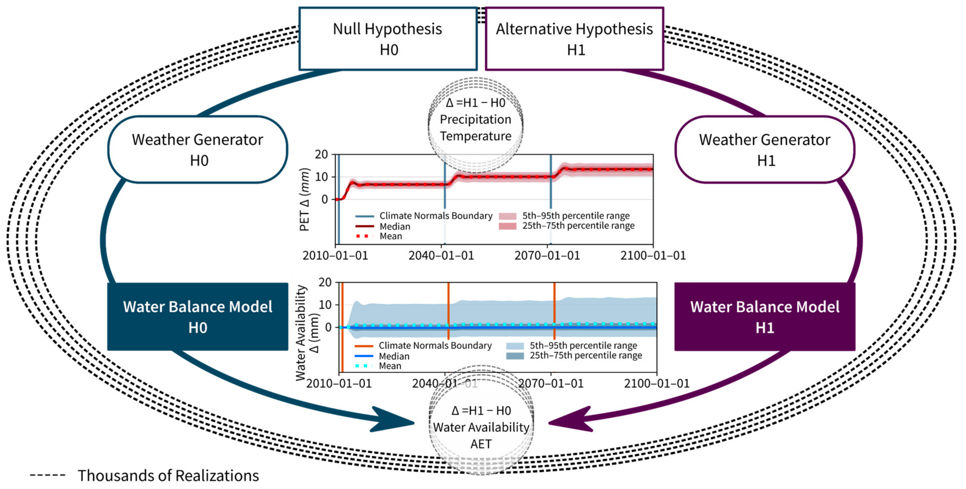
Martin [19] presents a framework for the assessment of relative risk to watershed-scale water resources from future systemic changes such as climate and LULC change. The framework provides a probabilistic risk assessment (PRA) that is composed of two simulation experiments, where one experiment, or pathway, represents reference conditions and is labeled the H0 pathway. The other pathway, labeled the H1 pathway, portrays the alternative hypothesis, which is a future projection of interference conditions. Actionable framework results are probabilistic differences, or ∆s where ∆ = H1 − H0, between pathway simulated values.
Each pathway contains two types of models: 1) a weather generator and 2) a water balance model. To isolate impacts on water availability from a particular systemic change, one model type should be identical in both pathways. The other model type should portray reference conditions in the H0 pathway and interference conditions in the H1 pathway.
Future interference conditions are uncertain and cannot be validated until they become historical observations. To address this inherent uncertainty, the framework employs Monte Carlo methods to simulate both pathways thousands of times to produce thousands of ∆ time histories. The collection of individual realizations is then converted to probabilistic ∆ time histories through the calculation of a cumulative histogram for each output time interval and the collation of individual percentile and mean results from each time interval cumulative mass function into probabilistic time histories.
The calculation of ∆ values isolates impacts on water resources to a specific systemic change. The emphasis on departures from reference conditions reduces the importance of traditional water balance model validation techniques that compare simulated results to observations for a different period than used for model calibration. Future interference conditions may represent change from reference conditions to the extent that historical model calibration is no longer fully relevant to the perturbed system. Because observations do not exist for future conditions, a water balance calculation should be conceptually validated to ensure that it produces the desired response across the range of weather forcing and watershed parameterization variations employed in future scenarios. The purpose of framing results in terms of departure, or ∆, values is to capture the change in response, not the absolute response, and to identify response changes with a specific forcing mechanism, either future climate trends or watershed parameterization.
A key feature of this PRA framework is the use of weather generators to convert from a scenario-based representation of future climate from GCM results for a single emissions scenario to an integrated future climate cone of uncertainty that includes multiple emissions scenarios. Two weather generators, one in each simulation pathway, provide a comparative analysis that ensures projected future climate trends are captured probabilistically. Several previous combined climate and LULC change analyses have employed a single weather generator to represent an individual emissions scenario [5,6,9].
Downscaled ensemble GCM results provide a limited (generally less than 100) set of realizations of future weather driven by hypothetical, future emissions scenarios. The goal of the ensemble representation is to bracket possible future conditions using multiple future emissions scenarios; it is not likely that a particular emissions scenario will provide an accurate prediction of actual emissions several decades in the future. Consequently, it is not plausible that ensemble members will provide an accurate prediction of daily or monthly weather for a particular day or month one or more years in the future.
The purpose of the ensemble is to provide insight into future climate through simulated and hypothetical future weather. Climate is the weather at a particular location averaged over an interval [20]. The concept of Climate Normals, three-decade averages of weather measures [21], can be used to convert GCM simulated future weather at a location to estimates of future climate, which are just expected or average future weather. A weather generator, simulating weather that reproduces expected climatic conditions, provides for thousands of realizations of future weather. This large collection of future weather realizations produces a continuous representation of the future climate cone of uncertainty in terms of likelihoods for future weather values.
This PRA framework provides a planning and management tool for water resource managers. It produces a description of future risk in terms of the magnitude of change in water availability and the quantification of likelihood for each change. This risk description provides the information required for the assessment of and planning for water resource sustainability and resiliency.
The PRA framework is implemented in this paper to analyze impacts on water availability from a combined climate and LULC change scenario for a small (less than 519 km2 or 200 mi2) watershed to provide a case study of framework formulation and to illustrate the advantages of the PRA approach. The advantages of PRA framework implementation relative to previous work examining future combined climate and LULC change are: (1) baseline, or reference, weather and future climate trends are converted to a continuous, probabilistic representation of weather, and there are no individual or separate reference climate and climate change scenarios; (2) the reference period concept is an integral framework component and not a separate scenario, which allows for presenting water availability results in terms of departures from reference conditions; and (3) framework outputs are cast in terms of relative risk to future water availability.
In the example implementation, future climate trends generate consistently unchanged median monthly water availability relative to historical weather conditions. However, average monthly water availability is expected to increase because of the inclusion of increased extreme event intensity in future climate trends, and these infrequent large magnitude events are sufficient to shift projected mean values. Impacts on water availability from LULC change are isolated and combined with impacts from future climate trends. Average and median monthly water availability are projected to increase under combined LULC and climate change. Average monthly water availability is estimated to increase by 1.1 times the increase projected from future climate trends.
2. Methods and Data
Martin [19] presented the PRA framework, shown in Figure 1, for analysis of the relative impact of future systemic changes on watershed-scale water resources and the identification of the uncertainty associated with projected impacts. This framework is employed to examine impacts on water availability from combined climate and LULC change. The same study site in west-central Texas, shown in Figure 2, that was used in Martin [19] is used to analyze impacts on water resources from a combined climate and LULC change scenario.
Table 1 presents the two future change scenarios assessed with the PRA framework. The results from these scenarios are compared to examine future impacts from climate change (CC) and combined LULC and climate change (LULCCC). As the 1981–2010 Climate Normals are different from those projected for 2011–2040 for the study site [19], it does not make sense to examine LULC change relative to reference conditions based on the 1981–2010 Climate Normals. Instead, LULC change conditions are examined in relation to existing watershed conditions, and future climate trends are used for weather forcing in both pathways in the LULCCC scenario.
2.1. Probabilistic Relative Impact Analysis Framework
The PRA framework, see Figure 1, is composed of two separate simulation pathways, or experiments, that are executed jointly within a probabilistic simulation structure. One pathway is the null hypothesis experiment (H0), representing reference conditions. The other pathway is the alternative hypothesis experiment (H1) that portrays interference, or future, conditions. Each pathway contains two models linked in series; a weather generator model produces synthetic weather forcing to drive a water balance model.
For framework implementation, weather-related or watershed parameterization-related interference conditions are isolated through the configuration of weather generator and water balance models between the experiments. One model-type should be the same in both pathways, and the other type should be different between pathways.
Probabilistic relative difference time histories are the framework outputs. Relative differences are labeled as ∆ values, and ∆ denotes the difference, ∆ = H1 − H0, between pathway simulated values. A probabilistic time history is a time series of probability distributions. ∆ time histories are flattened using a Butterworth filter [23] to reduce oscillations and facilitate multi-decade interpretation. This filtering approach generally flattens time histories but produces an oscillation at major slope changes such as the step transitions between Climate Normals. The presentation of framework results as relative differences isolates the impacts from the model type that is different between pathways, and reduces the possible influence of over-fitting or other systemic bias in the model type that is the same in both pathways.
2.2. Study Site
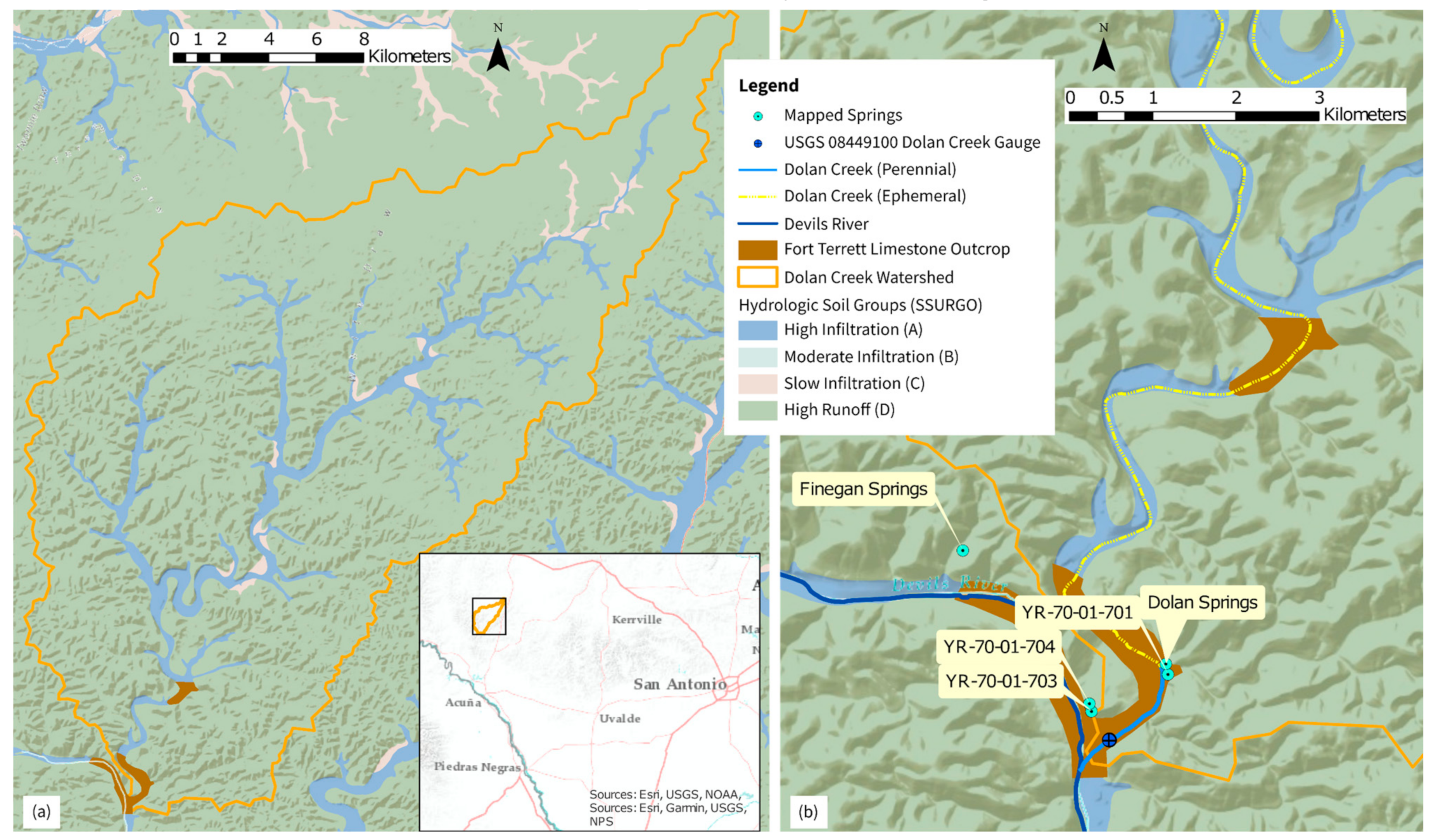
For the comparison of LULC change and climate change impacts, the 471 km2 Dolan Creek Watershed in Val Verde County, Texas (TX), USA (see Figure 2) is used as a study site. The coordinates of USGS 08449100, shown in Figure 2, in NAD83 are 29.888 degrees latitude and 100.990 degrees longitude. The watershed is in a remote part of Texas with little economic development. This region is currently, and is expected to remain through 2100, a hot semi-arid environment and BSh Köppen-Geiger climate classification [24].
The study site is at the intersection of the Edwards Plateau and Chihuahuan Desert biological regions; there are no paved roads within the watershed [25]. Because of the limited development, land cover across the watershed is relatively uniform shrub/scrub. Vegetation is predominately dry land scrub or shrublands. Common shrub types include creosote, juniper, and mesquite. Stands of trees, mainly oaks and sycamore, may be found adjacent to perennial rivers and streams [26,27].
The site is in karst terrain [28]. Most of the watershed is naturally impervious (hydrologic soil type D in Figure 2) with shallow to no soil. Valley bottom-areas exhibit enhanced secondary porosity from limestone dissolution and provide water storage capacity and elevated permeability, which produces the rapid infiltration rates for the valley bottom and dry stream bed locations. Additional details of the study site are available in Martin [19].
2.3. Water Balance Model
Any water budget calculation that uses precipitation and potential evapotranspiration (PET) as inputs, or internally calculates PET from temperature and site location, and produces actual evapotranspiration (AET), runoff, and recharge as outputs can be employed as a framework water balance model. In Martin [19], two types of water balance models are used. Here, the Hydrological Simulation Program—FORTRAN (HSPF) [29] continuous simulation, water balance model is used for the CC and LULCCC scenarios in Table 1.
HSPF provides for heterogeneous representation of the site watershed. It uses the concepts of hydrologic response units (HRUs) and hydrologic routing reservoirs for surface water bodies. Each HRU can be divided into a pervious component, or PERLND segment, and an impervious component, or IMPLND segment. Surface water bodies, including stream and river reaches are simulated with a well-mixed reservoir representation, or RCHRES components.
The RCHRES routing algorithm provides for up to five downstream exits; each exit can be used to direct water to a different destination. The default behavior is to utilize one exit that sends water downstream to the next reach. Seepage losses to groundwater can be represented using an additional designated exit.
IMPLND segments only represent the processes of AET and surface runoff. Because the land is impervious, there is no infiltration, percolation, or recharge.
In contrast, PERLND segments simulate a soil column with upper and lower zones. Surface runoff is the rainfall that is left over after infiltration, interception, AET during the storm, and depression storage. Infiltration occurs from the land surface into the upper zone and percolation is simulated from the upper to the lower zone. AET is calculated from both soil zones. Interflow is simulated as a loss from the lower soil zone which provides for delayed runoff to streams. Deep percolation, leaving the bottom of the soil column, exits the HSPF model as inactive groundwater inflow (IGWI).
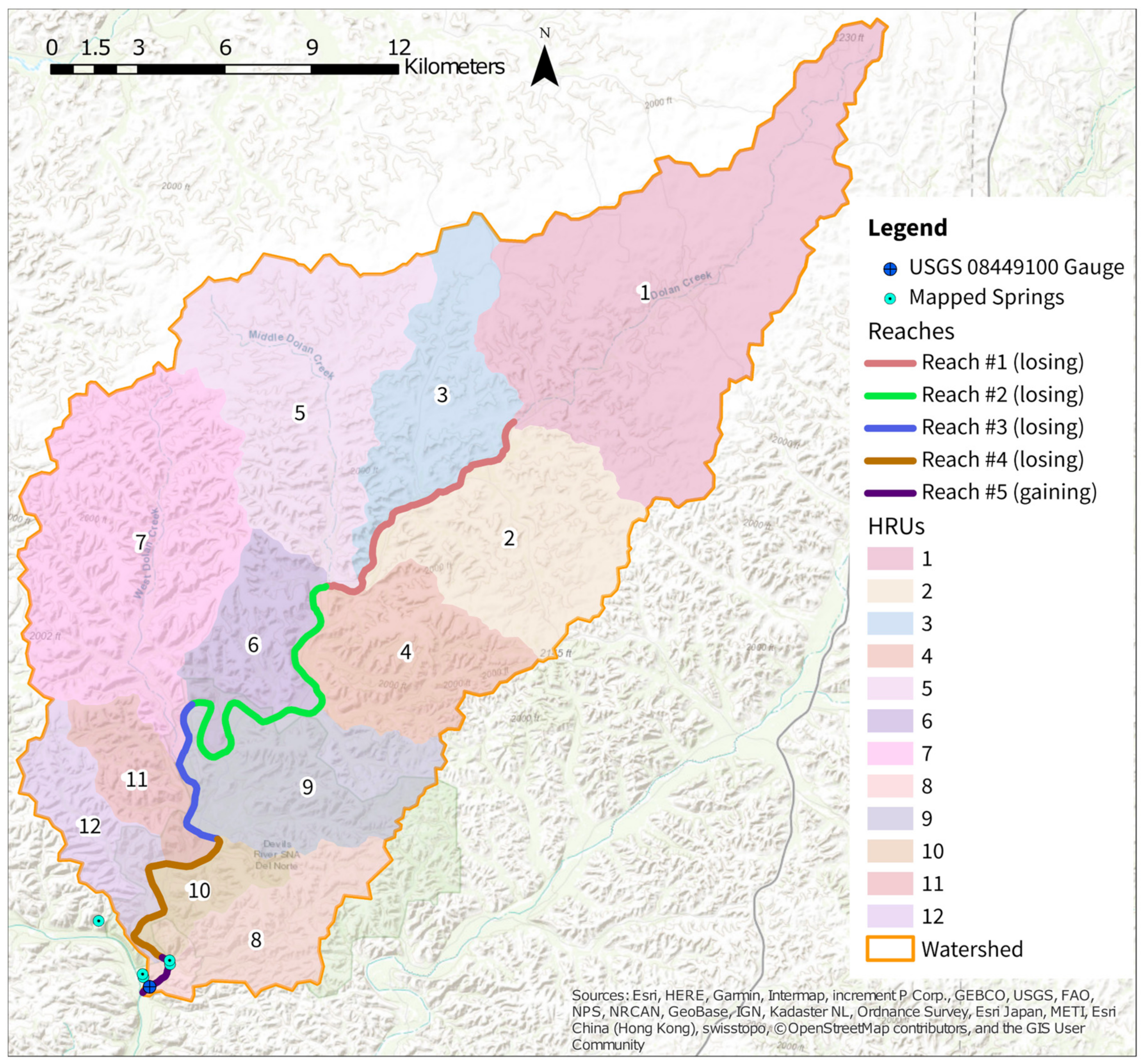
Figure 3 presents the HSPF model configuration for the study watershed. The watershed is divided into 12 HRUs and five stream segments. Runoff is routed to the nearest stream reach. For example, HRU 1, 2, and 3 runoff goes first to Reach 1, and runoff from HRU 10, 11, and 12 travels to Reach 4 and then downstream. Streamflow is routed along the stream from upstream (Reach 1) to downstream (Reach 5).
As shown in Figure 3, four of the stream segments are losing and one is gaining. Losing reaches are ephemeral and typically only contain water associated with recent rainfall. The perennial and gaining reach usually contains water. Typically, the water surface in the gaining reach is 10 to 13 m wide.
Because of the heterogeneous watershed depiction including gaining and losing stream reaches, the attribution of runoff and recharge from the HSPF model solution is complex. Recharge is calculated as the sum of IGWI from the pervious portion of HRUs and seepage losses from the four losing stream reaches in Figure 3. Runoff for the watershed is calculated as the discharge from Reach 5 to the model and basin outlet. As an example of complex flow patterns in the study watershed, runoff from HRU 1 and 2 goes to Reach 1; a portion of this runoff may become recharge in Reach 1 because of seepage losses.
Water availability is employed in preference to recharge and runoff components because of the complex flow patterns within the watershed. Although water availability is defined as precipitation less AET, it is calculated as the sum of runoff and recharge under the assumption that total precipitation will be approximately equal to the sum of total AET, recharge, and runoff across a thirty-year Climate Normals interval.
mHSP2 is the HSPF variant used for water balance modeling. It is one component of the pyHS2MF6 integrated hydrologic model [30]. mHSP2 was used for this study because the author had full access to and is intimately familiar with the source code. Access and knowledge of the source code facilitated the modifications required to implement the LULCCC scenario. mHSP2 had to be modified to represent changing pervious and impervious areas within an HRU during simulation time. The source code for mHSP2, as modified to implement the scenarios in Table 1, is available on the project GitHub (https://github.com/nmartin198/wres_risk_analysis, accessed on 24 February 2021).
2.4. Climate Change (CC) Scenario
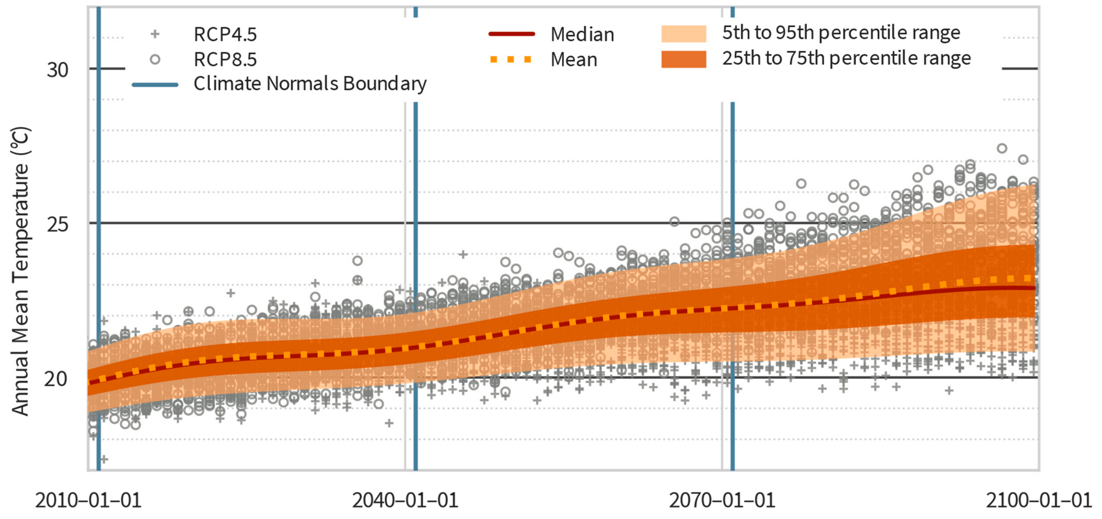
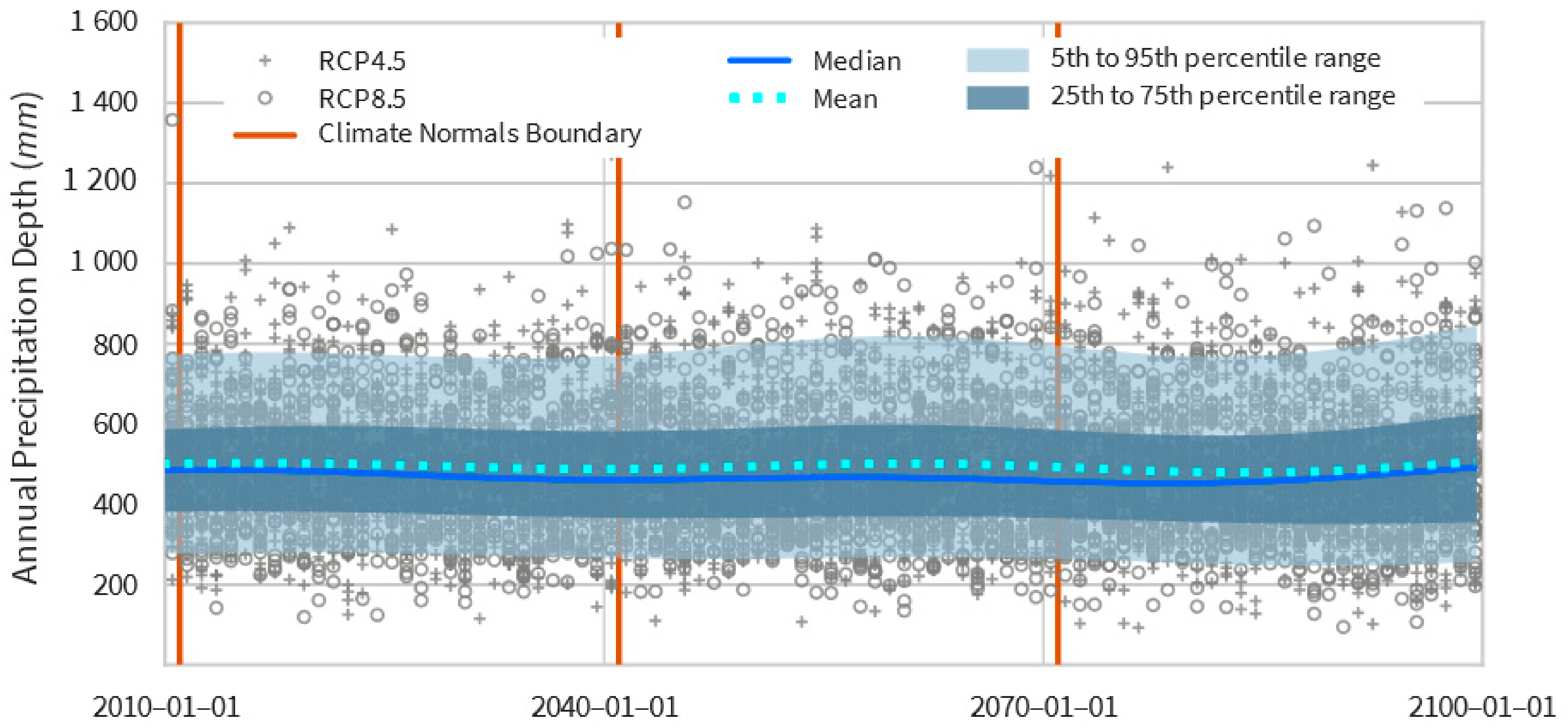
The CC scenario in Table 1 seeks to isolate the impacts of future climate trends on study site water resources. Analysis of future climate trends from downscaled GCM simulation results and the description, creation, and adjustment of the weather generator models are presented in Martin [19]. Figure 4 and Figure 5 display temperature and precipitation ensemble GCM simulation results for the study site from Representative Concentration Pathway (RCP) 4.5 and 8.5 emissions scenarios downscaled using the Localized Constructed Analogs (LOCA) [31] method. These downscaled ensembles were obtained from the “Downscaled CMIP3 and CMIP5 Climate and Hydrology Projections” archive [32,33].
Climate Normals, or three-decade averages of weather parameters, are used to convert GCM simulated weather to a climate description and to parameterize framework weather generators. Table 2 presents the three future Climate Normals simulated as part of the framework application.
As described in Table 1, identical water balance models are used in both pathways in this scenario. Different weather generators are used in each pathway for three projection intervals (2011–2040, 2041–2070, and 2071–2100). The H0 pathway weather generator is the same for all four intervals in Table 2, and it reproduces historical weather statistics. In the H1 pathway, the H0 weather generator is used for the “Data Interval”, and different weather generators are used for each projection interval in the H1 pathway, which seek to reproduce climate trends identified for that interval. The “Data Interval”, 1981–2010, is simulated to provide initial watershed conditions for the first projection interval, 2011–2040.
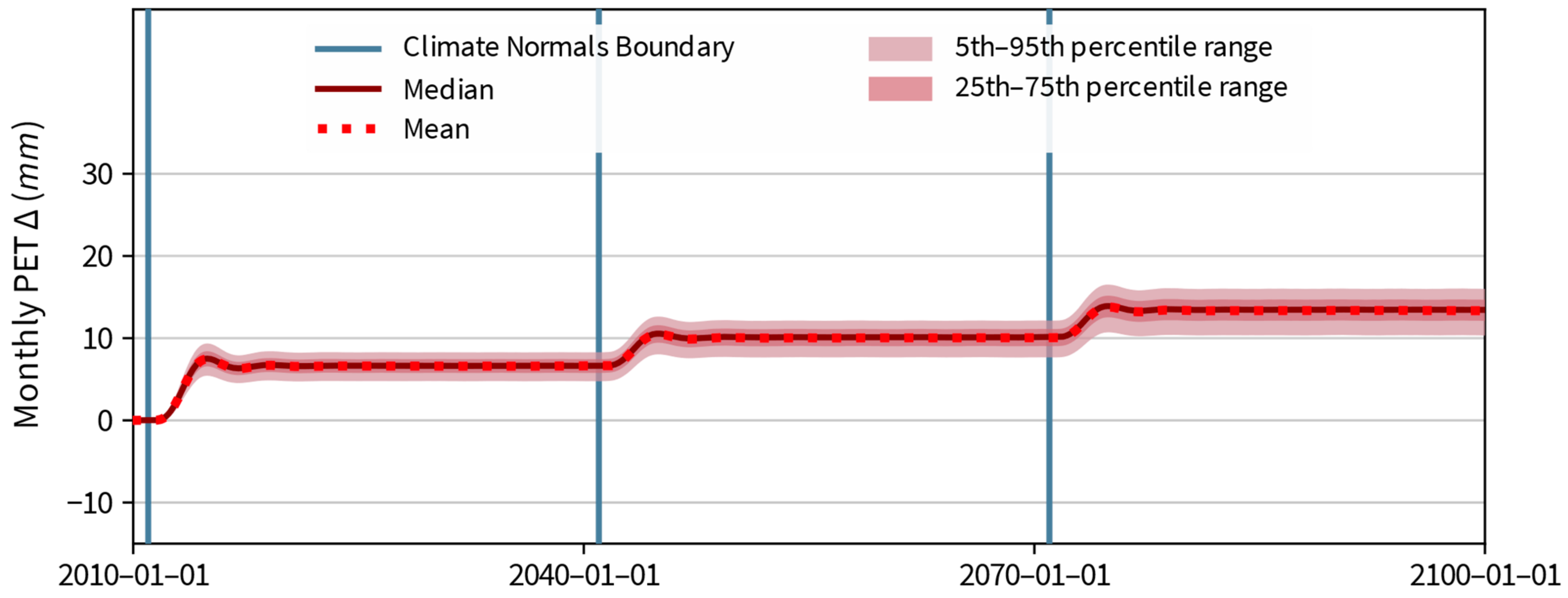
Projected climate trends for the site from 2011–2100, extracted from the analysis of downscaled GCM simulation results for multiple emissions scenarios, are a 3 °C increase in average temperature and a corresponding increase in potential evapotranspiration, no significant change in average annual precipitation, and a semi-arid classification from 2011–2100. Increases in extreme event intensity are represented for future conditions, producing low likelihood increases in precipitation amount and intensity during infrequent events [19].
Figure 6 and Figure 7 display probabilistic ∆ results for precipitation and PET from the framework for the CC scenario with 10,000 realizations. The probabilistic time histories presented in Figure 6 and Figure 7 provide the magnitude of projected change, ∆ values, and likelihoods per magnitude change over time. These results portray the future climate trends obtained via analysis of downscaled GCM simulation results for the study watershed.
The custom formulation of comparative weather generators within the framework was important for the simulation of future climate trends. Structural uncertainty issues of synthetic drizzle and the underprediction of extreme event magnitude in downscaled GCM simulation results for the watershed were identified from the comparison of simulation results and historical observations. The custom formulation allowed for trial-and-error adjustment of the H1 pathway weather generator to ameliorate these structural uncertainty issues. Without these custom adjustments, the propagation of too many wet days from synthetic drizzle through the weather generator formulation produced a future climate trend of a 30% increase in annual average precipitation from 2011–2100 [19].
The inclusion of the expectation for an increase in extreme event intensity during future Climate Normals into the H1 pathway weather generator is responsible for the positive skew in the 5th–95th percentile and interquartile ∆ ranges and for the positive bias in mean monthly ∆ in Figure 6. The median ∆ increases slightly but stays near zero in Figure 6; increased extreme event intensity has a relatively small impact on the median, in comparison to the mean, as would be expected from an infrequent increase in precipitation [19].
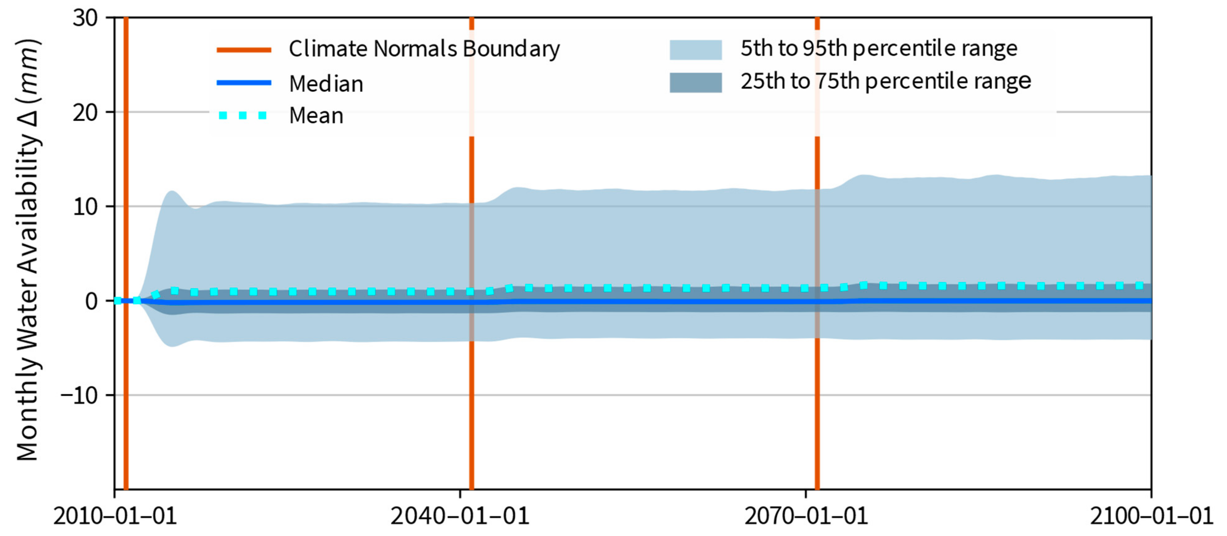
Water budget results for the CC scenario are presented in detail in Martin [19]. Here, the results are summarized to the extent needed for comparison with the LULCCC scenario. Figure 8 presents simulated probabilistic time histories of changes in water availability between future climate trends and historical conditions. Median expected change in future water availability is near zero because future annual average precipitation for the study site is expected to be unchanged. Mean water availability ∆ and the 5th–95th percentile range are positively biased because an increase in extreme event intensity is expected for future conditions. The 5th–95th percentile range provides a description of variability in simulated water availability ∆s. During 2071–2100, simulated average mean water availability ∆ is 1.6 mm, and average median water availability ∆ is 0.0 mm. The mean is positive and the median is zero because of the contribution to monthly precipitation depth from infrequent extreme events.
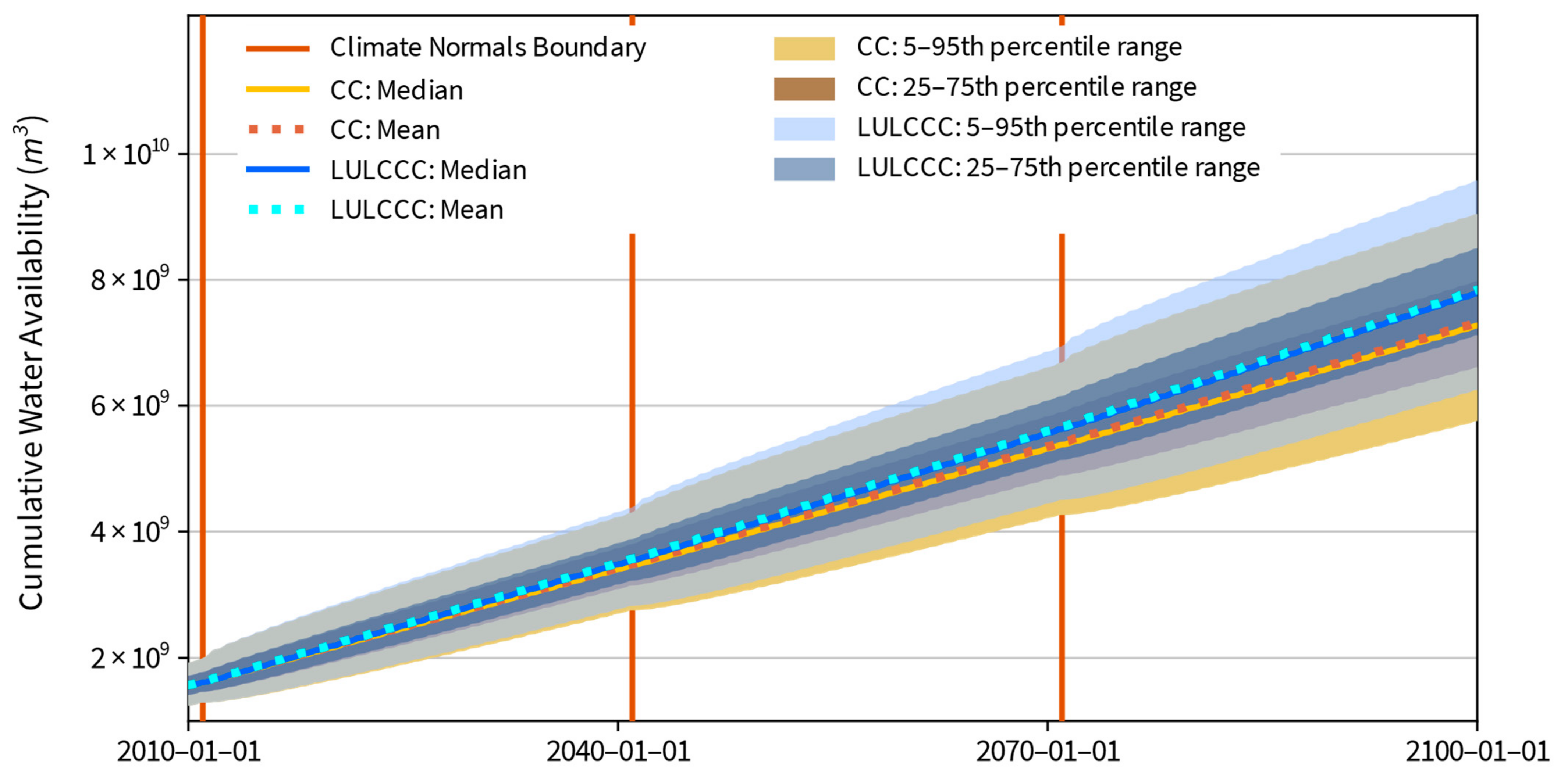
Figure 9 displays a probabilistic description of cumulative water availability across the simulation time defined in Table 2. The slope of average and median cumulative water availability is consistent across the future intervals, denoting no change to expected precipitation depth on an annual basis.
Water budget component results for HRU 1 and 2 and Reach 1 and 5 are provided in Table 3 and Table 4. These results are presented for comparison with LULCCC scenario results. In these tables, average monthly median and 5th, 25th, 75th, and 95th percentile ∆ values are presented as a dimensionless, normalized score using Equation (1). For a symmetrical distribution of ∆ values, the median normalized score (Sn) is expected to be close to zero, denoting that the median and mean are close in value. The 25th percentile Sn should be approximately −0.5, and the 75th percentile should be about 0.5.
| Sn = normalized score, dimensionless | x∆ = monthly average difference statistic |
| m∆ = mean monthly average difference | IQR∆ = monthly average interquartile range |
2.5. Land Use and Land Cover (LULC) Change Scenario
A future economic development hypothesis was used to create the LULC change portion of the LULCCC scenario in Table 1. This hypothesis postulates a 10% increase in developed area for HRUs 1 and 2 across each future analysis interval in Table 2. HRUs 1 and 2 were selected for development because these two regions were the primary locations of energy-related development between 2001 and 2016 [25], and these two regions are in proximity to the nearest major road.
Developed areas are assumed to be impervious. Increased impervious surface area changes the landscape from an infiltrative sink to a source of runoff because infiltration is eliminated for impervious surfaces [34,35]. Table 5 provides the corresponding change in impervious area for HRUs 1 and 2 across 2011–2100. Impervious areas are represented as IMPLND segments, which only provide for simulation of surface runoff and evaporation from surface depressions, in the HSPF model.
As described in Table 1, identical weather generator models are used in both pathways in this scenario; this weather generator represents projected climate trends from 2011–2100. Different water balance model parameterization is used in each pathway. The H0 pathway water balance model represents existing conditions, and parameterization is constant for all four intervals in Table 2. In the H1 pathway, the existing conditions parameterization is used for the water balance model during the “Data Interval”. The parameterization of the water balance model in the H1 pathway is varied according to Table 5 for three projection intervals (2011–2040, 2041–2070, and 2071–2100). The “Data Interval”, 1981–2010, is simulated to provide identical initial watershed conditions for the first projection interval, 2011–2040, when model parameterization and model results in the two pathways begin to diverge.
3. Results
The PRA framework in Figure 1 was applied to the LULCCC scenario in Table 1 to compare risks to watershed-scale water resources from climate change and from hypothetical future land use modifications combined with climate change.
3.1. Combined Land Use, Land Cover and Climate Change (LULCCC) Scenario
The LULC change portion of this scenario utilizes an increase in impervious area in HRU 1 and 2 (see Figure 3), as described in Table 5, to represent future economic development. Identical weather generators, which reproduce future climate trends, are used in both pathways and provide for the climate change portion of the scenario. The HSPF models are different between pathways. The H0 pathway HSPF model is parameterized to represent existing conditions, and the parameterization of the H1 pathway HSPF model varies across simulation time to portray LULC change.
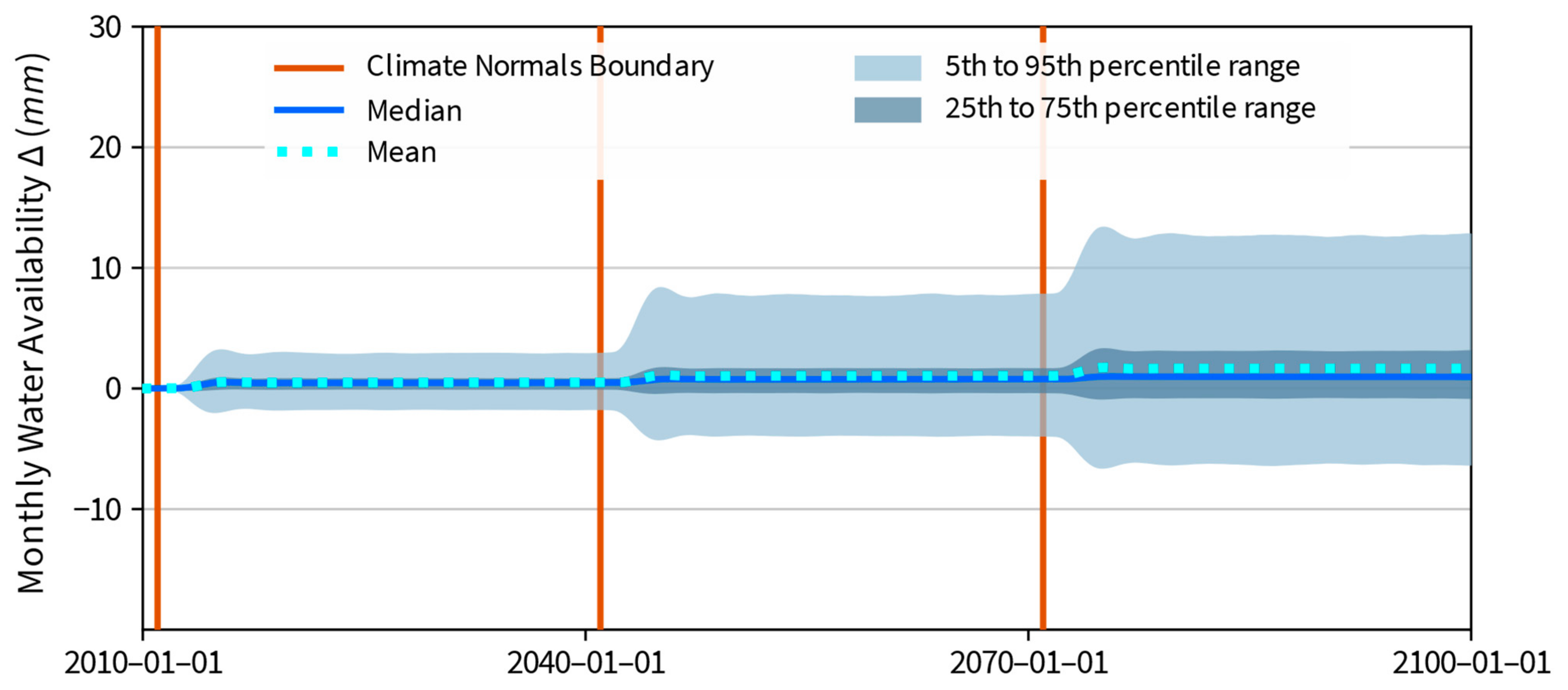
Figure 10 shows the simulated change in water availability, and corresponding likelihoods, across the three future Climate Normals. An increase in impervious area in HRU 1 and 2 is represented in this scenario as a stepwise percentage increase in area, which produces the stepped increases in mean water availability ∆ and the 5th–95th percentile range. During 2070–2100, monthly average mean water availability ∆ is 1.7 mm, and monthly average median water availability ∆ is 1.0 mm, corresponding to expected monthly increases in water availability of 8.01E+05 m3 and 4.71E+05 m3, respectively. These monthly increases in water availability are for the LULCCC scenario relative to the CC scenario, and represent increased water availability from LULC change independent of climate change.
Figure 9 displays the cumulative water availability cone of uncertainty for the LULCCC scenario. The slope of cumulative mean water availability increases at each Climate Normals boundary due to the stepwise increase in impervious area. The LULCCC cumulative mean water availability is larger than the CC cumulative mean from 2040–2100, and it stays within the CC cumulative water availability interquartile range, “CC: 25–75th percentile range”, from 2011–2100.
The cumulative water availability, shown in Figure 9, and the water availability ∆ time histories, shown in Figure 10, apply to the entire study watershed (see Figure 2). In the LULCCC scenario, impervious area is increased in HRU 1 and 2 (see Figure 3), which comprise approximately 31% of the total watershed area.
Because LULC changes affect HRU 1 and 2, these are the only HRUs that have simulated changes to the distribution of the water balance components of AET, recharge, and runoff. Table 6 provides the relative change in AET, runoff, and recharge for HRU 1 and 2 under the LULC changes. The results are similar for the HRUs and are proportional to the relative area; HRU 2 has about 42% of the HRU 1 watershed area. Increased impervious area produces increased runoff, denoted by positive mean values in Table 6. Mean AET and recharge both decrease given LULC changes. Increases in runoff are generated at the expense of AET and recharge, which both decrease with increases in impervious area.
Runoff from HRU 1 and 2 is routed to Reach 1 (see Figure 3). Discharge from Reach 1 continues downstream to Reach 2, Reach 3, Reach 4, and Reach 5 in series. Table 7 displays relative change in evaporation, discharge, and seepage from Reach 1 and 5 from LULC changes. In Reach 1, seepage and evaporation both increase because this ephemeral reach is typically dry; additional runoff means that more water is available for evaporation and seepage. The increase in Reach 1 discharge downstream is larger than the combined increase in seepage and evaporation. Reach 5 is a gaining reach and has no seepage losses. Upstream seepage losses from Reaches 1, 2, 3, and 4 mute the increase in discharge from the watershed relative to the increase in runoff from HRU 1 and 2. As Reach 5 is gaining and perennial, the reach is always wet; water is available for evaporation, and evaporation is not water supply limited. Consequently, there is negligible relative change to Reach 5 evaporation.
3.2. Scenario Comparison
The PRA framework, see Figure 1, contains two simulation experiments. Each experiment includes a weather generator and water balance model. To isolate risks associated with a particular driving mechanism, only one type of model should be different between the pathways. For the CC scenario, the weather generator models are different between pathways. In the LULCCC scenario, the water balance models are different between pathways. The LULCCC H0 water balance model is the same as the water balance models used in the CC scenario. A water balance model that has a time varying representation of impervious area extent is used in the LULCCC H1 pathway.
In the CC scenario, monthly average mean water availability ∆ is 1.6 mm during 2070–2100, corresponding to a monthly increase of 7.54 × 10⁵ m3 in water availability given future climate trends. Average monthly water availability is expected to increase because of the inclusion of increased extreme event intensity in the future climate representation. The mean monthly runoff ∆ in Table 3 is larger than the 75th percentile runoff ∆ for HRU 1 and 2. Monthly average median water availability ∆ is 0.0 mm in 2070–2100 for the CC scenario. The monthly change in median water availability is zero because average annual precipitation is not expected to change from 2011–2100.
The LULCCC scenario employs the climate change weather generator in both pathways, and different water balance model parameterization in each pathway. The H1 water balance model uses an impervious area parameterization that changes among Climate Normals, as described in Table 5. An increase in impervious area results in an increase in runoff, a decrease in recharge, and a decrease in AET. The overall impact on the site watershed is to increase average water availability under future interference conditions, resulting in a positive bias in mean and median water availability ∆s in Figure 10.
Monthly average mean water availability is expected to increase by 8.01 × 10⁵ m3 during 2071–2100. Similarly, monthly average median water availability increases 4.71 × 10⁵ m3. Median monthly water availability is expected to increase by 4.71 × 10⁵ m3 in the LULCCC from the 0 m3 increase hypothesized for future climatic conditions relative to observed weather in the CC scenario.
A shift in expected values for runoff, AET, and recharge water budget components occurs for the HRUs, whose impervious area increases are shown in Table 5. Runoff increases with increases in impervious area, while AET and recharge decrease. For the study site, the LULCCC scenario provides a change in the median water budget. The CC scenario generates increased variability in lower likelihood conditions such as the 5th and 95th percentile ∆s, and suggests an infrequent increase in water availability from increased extreme event intensity that creates a positive bias in mean water availability ∆s.
4. Discussion
A PRA framework is described for the analysis of water resource impacts from systemic change. It is applied to an examination of combined LULC and climate change impacts on water resources for a small watershed in west-central Texas.
The study site is in karst terrain and has complex, interrelated surface and sub-surface flow paths. A heterogenous water balance model representation including 12 HRUs and five stream reaches is used to partition precipitation into AET, recharge, and runoff components. Water availability is calculated as the sum of recharge and runoff. Runoff for the entire watershed is calculated as the discharge from Reach 5 to the watershed outlet. Recharge is attributed to the sum of deep percolation to inactive groundwater from the pervious portion of each HRU and seepage from losing stream reaches. Recharge is defined as water that percolates across the water table of an aquifer [36]; water tables are not explicitly simulated in the water balance model.
Within complex watershed flow paths, runoff from headwaters HRUs such as HRU 1 and 2 is routed to a stream reach where a portion of the runoff could be lost to seepage. In this accounting, seepage is attributed to recharge. Deep percolation in pervious areas is also attributed to recharge. There are numerous springs in and adjacent to the study watershed (see Figure 2). Some of this deep percolation may never reach a water table and instead travel through preferential flow pathways to discharge as spring flow or discharge into a gaining stream reach. Because of complex flow paths and a lack of explicit water table simulation, the concept of water availability is preferred for study site water resources. An attempt to delineate recharge and runoff components would be arbitrary for this study area because a drop of water falling on the headwaters pervious lands may be categorized as both recharge and runoff at different points in the journey to the outlet and may switch categories multiple times.
4.1. Novelty of the PRA Framework Approach
The PRA framework is general in the sense that it can be customized and applied to any site for water resource risk analysis. Generic weather generators can be parameterized to represent site specific climate and utilized within the framework. Any water balance model that accepts precipitation and PET, or calculates PET from site location and temperature, as inputs can be used within the framework.
The novel contributions of and benefits from the PRA approach are associated with the use of two simulation pathways within a probabilistic simulation framework. The H0 pathway portrays reference conditions, and the H1 pathway represents future conditions. Reference conditions are an integral component of the framework and not a separate scenario. Relative results from the pathways, or ∆ time histories, are presented using the magnitude of departure from reference conditions and likelihood of departure magnitude.
Comparative analysis of reference, or historical, weather generator results with simulated future climate weather generator results provides a mechanism to ensure that identified future climate trends are reproduced. The probabilistic representation of future climate allows for the incorporation of results from multiple emissions scenarios because overlapping precipitation and temperature values among scenarios are considered more probable because of the higher frequency of occurrence. If needed, the H1 weather generator can be adjusted to produce the desired, relative future trends, and it can be augmented to represent hypotheses that are missing from downscaled ensemble GCM simulation results. In the CC scenario, the H1 weather generator representation was adjusted to ameliorate synthetic drizzle issues evident in downscaled ensemble GCM simulation results for the study site. The H1 weather generator was also augmented to portray increased extreme event intensity in future Climate Normals that was not present in downscaled GCM simulation results for the site watershed.
Probabilistic comparative water balance model results are beneficial for the analysis of future conditions. The casting of results in terms of departures from reference conditions removes the focus from absolute simulated quantities and reduces the importance of traditional calibration and validation considerations. Interference conditions likely represent significant systemic change relative to reference conditions, and observations do not exist for future conditions. These special considerations for the simulation of future conditions reduce the applicability of approaches designed for the reproduction of historical and stationary conditions. A water balance calculation should be conceptually validated to ensure that it produces the desired response across the range of weather forcing and watershed parameterization variations employed in interference scenarios, prior to incorporation in the framework.
The purpose of this framework is to provide a planning and analysis tool for water resource managers. It describes water resource risk in terms of magnitude of change in water availability and provides quantification of the likelihood for each change. This risk description provides useful information for water resource sustainability and resiliency analyses.
4.2. Limitations of the Study and Future Research Tasks
Projections of combined future LULCCC impacts, climate change impacts, and the comparison of impacts between future LULCCC and CC scenarios are site-specific and only include water availability considerations. Temperatures are expected to increase by 1.5 °C across the world between 2030 and 2052 relative to pre-industrial levels, and changes to precipitation are projected to be region dependent, with increased precipitation intensity in some areas and increased probability of drought in several regions [37]. Temperatures at the study site are expected to increase; however, the expectation is for minimal change to average annual precipitation [19]. The study site is currently, and is projected to remain through 2100, a hot semi-arid environment [24]. Projected impacts on water availability from future climate trends are controlled by the specific future climate projections for this location.
The PRA framework is designed for the analysis of impacts from future systemic changes and is built to deal with the inherent uncertainty in future interference conditions. When data and observations are available to guide and constrain impact analyses from systemic change (i.e., for historical changes), more direct and robust analysis approaches should be used.
LULC change can affect weather and climate because it may modify surface fluxes of heat and water vapor and impact the energy available for storms [2]. The PRA framework is configured to propagate future climate trends through a water balance model, in one direction, to produce relative change in water availability. Feedback from the water balance model representation back to the weather generator, to represent LULC change feedback to climate, is not available in the framework formulation.
The LULCCC scenario assumes a consistent increase in economic development within the site watershed. Rather than assuming an LULC change scenario, LULC could have been modeled using cellular automata-based [4,6,16,38] or similar methods. Minimal alteration and land use change have occurred in the watershed historically; consequently, advanced LULC modeling is not likely to provide significant improvements for the representation of this site. In future applications, the PRA framework could incorporate a water balance model that is parameterized in future intervals in accordance with projections obtained from LULC change models.
Only impacts on water availability are examined in the case study. It is possible that water availability could increase but that water quality could be negatively impacted by increased economic development. In future framework applications, water quality considerations can be incorporated into the formulation. One way to include water quality considerations would be to use HSPF water balance models that include transport and water quality representations [5,12,16]. The PRA framework is amenable to the inclusion of many different types of water balance models, and ecohydrology analysis models could be used within the framework instead of HSPF. In either approach, ∆ time histories could be produced for water quality and ecohydrology parameters and metrics in addition to water budget components.
4.3. Implications for Sustainable Water Management
Watershed sustainability can be defined and described using social, environmental, and biodiversity indicators [39]. The PRA framework only provides analysis of impacts on the watershed water balance; consequently, it does not, by itself, provide for analysis of water management sustainability or resiliency. The PRA framework does produce a description of future risk in terms of magnitude of change in water availability and the quantification of likelihood for each change. The combination of change in water availability and the probability of change provides important contributing information for the analysis of water resource sustainability and resiliency. The PRA framework can provide a tool to describe expected water resource availability that can be incorporated into a larger decision support system that considers investment and engagement strategies and long-term integrated resource management approaches.
5. Conclusions
A PRA framework is described for the analysis of future systemic impacts on watershed-scale water resources and implemented to analyze combined LULC and climate change impacts for a study site in west-central TX. The PRA framework provides the advantages of the intrinsic incorporation of climate change projections and reference conditions into framework analysis. This produces a combined LULC and climate change assessment where only LULC scenarios are examined as opposed to a combination of future climate change and LULC scenarios.
The example implementation provides a site-specific analysis of impacts from LULC and climate change. It projects that future climate trends do not significantly change expected water availability; however, low probability, extreme events are predicted to produce low frequency increases in water availability. An LULC change scenario involving a constant increase in economic development, with a corresponding increase in impervious area, of 10% every 30 years for two watershed subareas is examined in conjunction with climate change. Water availability is forecast to increase on average by 1.1 times under LULC conditions relative to climate change conditions.
Supplementary Materials
The following are available online at https://0-www-mdpi-com.brum.beds.ac.uk/2306-5338/8/1/38/s1. Figure S1. HRU 1 magnitude of change in runoff and associated likelihoods for both scenarios. Figure S2. HRU 1 magnitude of change in AET and associated likelihoods for both scenarios. Figure S3. HRU 1 magnitude of change in recharge and associated likelihoods for both scenarios. Figure S4. Reach 1 magnitude of change in discharge to Reach 2 and associated likelihoods for both scenarios. Figure S5. Reach 1 change in seepage and associated likelihoods for both scenarios. Figure S6. Reach 1 change in evaporation for both scenarios. Figure S7. Reach 5 magnitude of change in discharge downstream and out of the model and associated likelihoods for both scenarios. Table S1. Listing of the 32 GCMs and Emission Scenarios available in the CMIP5, LOCA Archive.
Author Contributions
The author is responsible for conceptualization, methodology, software, validation, formal analysis, investigation, writing, visualization, project administration, and funding acquisition. The author has read and agreed to the published version of the manuscript.
Funding
This research was funded by Southwest Research Institute® (SwRI), Internal Research and Development Grant 15-R8937.
Institutional Review Board Statement
Not applicable.
Informed Consent Statement
Not applicable.
Data Availability Statement
Publicly available datasets were analyzed in the Martin [19] companion study. These data can be found at: https://gdo-dcp.ucllnl.org/downscaled_cmip_projections/dcpInterface.html and https://prism.oregonstate.edu/explorer/.
Acknowledgments
The author would like to acknowledge the guidance of four anonymous reviewers that provided beneficial suggestions that improved the quality of this paper. Additionally, the author would like to recognize the contributions of G. Firmani, who provided several invaluable, preliminary reviews of this work. The author would also like to acknowledge the World Climate Research Programme’s Working Group on Coupled Modelling. The author thanks the climate modeling groups (listed in Table S1 of this paper) for producing and making available their model output. For CMIP, the U.S. Department of Energy’s Program for Climate Model Diagnosis and Intercomparison provides coordinating support and led the development of software infrastructure in partnership with the Global Organization for Earth System Science Portals.
Conflicts of Interest
The author declares no conflict of interest.
Computer Code and Software
Custom HSPF model code to implement the LULCCC scenario and scripts, Jupyter Notebooks, and model input and output files used for this study are available on the project GitHub site at: https://github.com/nmartin198/wres_risk_analysis.
References
- Theodore, L.; Dupont, R.R.; Future, U.S. Water security. In Water Resource Management Issues: Basic Principles and Applications; CRC Press: Boca Raton, FL, USA, 2019; p. 8. ISBN 978-0-429-06127-1. [Google Scholar]
- Pielke, R.A. Land use and climate change. Science 2005, 310, 1625–1626. [Google Scholar] [CrossRef] [Green Version]
- Gorelick, D.E.; Lin, L.; Zeff, H.B.; Kim, Y.; Vose, J.M.; Coulston, J.W.; Wear, D.N.; Band, L.E.; Reed, P.M.; Characklis, G.W. Accounting for adaptive water supply management when quantifying climate and land cover change vulnerability. Water Resour. Res. 2020, 56, e2019WR025614. [Google Scholar] [CrossRef]
- Dibaba, W.T.; Demissie, T.A.; Miegel, K. Watershed hydrological response to combined land use/land cover and climate change in highland Ethiopia: Finchaa catchment. Water 2020, 12, 1801. [Google Scholar] [CrossRef]
- Vaighan, A.A.; Talebbeydokhti, N.; Bavani, A.M. Assessing the impacts of climate and land use change on streamflow, water quality and suspended sediment in the Kor River Basin, Southwest of Iran. Environ. Earth Sci. 2017, 76, 543. [Google Scholar] [CrossRef]
- Yan, R.; Cai, Y.; Li, C.; Wang, X.; Liu, Q. Hydrological responses to climate and land use changes in a watershed of the loess plateau, China. Sustainability 2019, 11, 1443. [Google Scholar] [CrossRef] [Green Version]
- Zhang, L.; Nan, Z.; Yu, W.; Ge, Y. Hydrological responses to land-use change scenarios under constant and changed climatic conditions. Environ. Manag. 2016, 57, 412–431. [Google Scholar] [CrossRef] [PubMed]
- Zipper, S.C.; Motew, M.; Booth, E.G.; Chen, X.; Qiu, J.; Kucharik, C.J.; Carpenter, S.R.; Loheide, S.P., II. Continuous separation of land use and climate effects on the past and future water balance. J. Hydrol. 2018, 565, 106–122. [Google Scholar] [CrossRef] [Green Version]
- Willuweit, L.; O’Sullivan, J.J.; Shahumyan, H. Simulating the effects of climate change, economic and urban planning scenarios on urban runoff patterns of a metropolitan region. Urban. Water J. 2016, 13, 803–818. [Google Scholar] [CrossRef]
- Tu, J. Combined impact of climate and land use changes on streamflow and water quality in Eastern Massachusetts, USA. J. Hydrol. 2009, 379, 268–283. [Google Scholar] [CrossRef]
- Martin, K.L.; Hwang, T.; Vose, J.M.; Coulston, J.W.; Wear, D.N.; Miles, B.; Band, L.E. Watershed impacts of climate and land use changes depend on magnitude and land use context. Ecohydrology 2017, 10, e1870. [Google Scholar] [CrossRef]
- Praskievicz, S.; Chang, H. Impacts of climate change and urban development on water resources in the Tualatin River Basin, Oregon. Ann. Assoc. Am. Geogr. 2011, 101, 249–271. [Google Scholar] [CrossRef]
- Hung, C.-L.J.; James, L.A.; Carbone, G.J.; Williams, J.M. Impacts of combined land-use and climate change on streamflow in two nested catchments in the Southeastern United States. Ecol. Eng. 2020, 143, 105665. [Google Scholar] [CrossRef]
- Kim, J.; Choi, J.; Choi, C.; Park, S. Impacts of changes in climate and land use/land cover under IPCC RCP scenarios on streamflow in the Hoeya River Basin, Korea. Sci. Total Environ. 2013, 452–453, 181–195. [Google Scholar] [CrossRef]
- Pan, Z.; He, J.; Liu, D.; Wang, J. Predicting the joint effects of future climate and land use change on ecosystem health in the middle reaches of the Yangtze River Economic Belt, China. Appl. Geogr. 2020, 124, 102293. [Google Scholar] [CrossRef]
- Tong, S.T.Y.; Sun, Y.; Ranatunga, T.; He, J.; Yang, Y.J. Predicting plausible impacts of sets of climate and land use change scenarios on water resources. Appl. Geogr. 2012, 32, 477–489. [Google Scholar] [CrossRef]
- Sinha, R.K.; Eldho, T.I.; Subimal, G. Assessing the impacts of historical and future land use and climate change on the streamflow and sediment yield of a tropical mountainous river basin in South India. Environ. Monit. Assess. 2020, 192, 679. [Google Scholar] [CrossRef] [PubMed]
- Zeng, F.; Ma, M.-G.; Di, D.-R.; Shi, W.-Y. Separating the impacts of climate change and human activities on runoff: A review of method and application. Water 2020, 12, 2201. [Google Scholar] [CrossRef]
- Martin, N. Watershed-scale, probabilistic risk assessment of water resources impacts from climate change. Water 2021, 13, 40. [Google Scholar] [CrossRef]
- National Snow and Ice Data Center (NSIDC). Climate Weather; National Snow and Ice Data Center: Boulder, CO, USA, 2020. [Google Scholar]
- National Centers for Environmental Information (NCEI). Climate Normals; National Centers for Environmental Information: Asheville, NC, USA, 2020. [Google Scholar]
- The SciPy Community Scipy. Signal.Butter—SciPy v1.6.0 Reference Guide. Available online: https://docs.scipy.org/doc/scipy/reference/generated/scipy.signal.butter.html (accessed on 20 January 2021).
- Beck, H.E.; Zimmermann, N.E.; McVicar, T.R.; Vergopolan, N.; Berg, A.; Wood, E.F. Present and future Köppen-Geiger climate classification maps at 1-Km resolution. Sci. Data 2018, 5. [Google Scholar] [CrossRef] [Green Version]
- Wickham, J.; Homer, C.; Vogelmann, J.; McKerrow, A.; Mueller, R.; Herold, N.; Coulston, J. The Multi-Resolution Land Characteristics (MRLC) Consortium—20 years of development and integration of USA national land cover data. Remote Sens. 2014, 6, 7424–7441. [Google Scholar] [CrossRef] [Green Version]
- U.S. Geological Survey LANDFIRE. LANDFIRE Existing Vegetation Type; U.S. Geological Survey: Millersburg, MI, USA, 2016.
- U.S. Geological Survey LANDFIRE. LANDFIRE National Vegetation Classification Layer; U.S. Geological Survey: Millersburg, MI, USA, 2016.
- Barker, R.A.; Bush, P.W.; Baker, E.T. Geologic History and Hydrogeologic Setting of the Edwards-Trinity Aquifer System, West-Central Texas; Water-Resources Investigations Report 94-4039; U.S. Geological Survey: Austin, TX, USA, 1994; ISBN 3-901503-77-3.
- Bicknell, B.R.; Imhoff, J.C.; Kittle, J.L., Jr.; Donigan, A.S., Jr.; Johanson, R.C.; Barnwell, T.O. Hydrological Simulation Program—Fortran User’s Manual for Release 11; U.S. Environmental Protection Agency: Washington, DC, USA, 1996; Volume 100.
- Natural Resources Conservation Service Soils (NRCS). Description of SSURGO Database; Natural Resources Conservation Service Soils: Chestertown, MD, USA, 2020.
- Martin, N. Nmartin198/PyHS2MF6—PyHS2MF6: An Integrated Hydrologic Model; GitHub: San Francisco, CA, USA, 2021. [Google Scholar]
- Pierce, D.W.; Cayan, D.R.; Thrasher, B.L. Statistical Downscaling Using Localized Constructed Analogs (LOCA). J. Hydrometeorol. 2014, 15, 2558–2585. [Google Scholar] [CrossRef]
- Brekke, L.; Thrasher, B.L.; Maurer, E.P.; Pruitt, T. Downscaled CMIP3 and CMIP5 Climate Projections: Release of Downscaled CMIP5 Climate Projections, Comparison with Preceding Information, and Summary of User Needs; Southwest Climate Adaptation Science Center (SW CASC): Tucson, AZ, USA, 2013; p. 47. [Google Scholar]
- Bracken, C. Downscaled CMIP3 and CMIP5 Climate Projections-Addendum Release of Downscaled CMIP5 Climate Projections (LOCA) and Comparison with Preceding Information; Southwest Climate Adaptation Science Center (SW CASC): Tucson, AZ, USA, 2016; p. 29. [Google Scholar]
- Booth, D.B.; Jackson, C.R. Urbanization of aquatic systems: Degradation thresholds, stormwater detection, and the limits of mitigation1. J. Am. Water Resour. Assoc. 1997, 33, 1077–1090. [Google Scholar] [CrossRef]
- Pan, F.; Choi, W.; Choi, J. Effects of urban imperviousness scenarios on simulated storm flow. Environ. Monit Assess. 2018, 190, 499. [Google Scholar] [CrossRef]
- Freeze, A.R.; Cherry, J.M. Groundwater; Pearson: London, UK, 1979; ISBN 978-0-13-365312-0. [Google Scholar]
- IPCC. Global Warming of 1.5 °C. An IPCC Special Report on the Impacts of Global Warming of 1.5°C above Pre-Industrial Levels and Related Global Greenhouse Gas. Emission Pathways, in the Context of Strengthening the Global Response to the Threat of Climate Change; Intergovernmental Panel on Climate Change (IPCC): Geneva, Switzerland, 2018; Volume 2, p. 630. [Google Scholar]
- Choi, W.; Pan, F.; Wu, C. Impacts of climate change and urban growth on the streamflow of the Milwaukee River (Wisconsin, USA). Reg. Environ. Chang. 2017, 17, 889–899. [Google Scholar] [CrossRef]
- Sood, A.; Ritter, W.F. Developing a framework to measure watershed sustainability by using hydrological/water quality model. J. Water Resour. Prot. 2011, 3, 788–804. [Google Scholar] [CrossRef] [Green Version]
Figure 1.
Systemic change, relative impact analysis framework for watershed-scale water resources. Framework results are presented in terms of probabilistic differences, or ∆s (∆ = H1 − H0). Use of ∆ values allows for isolation of impacts on water resources from interference conditions. Potential evapotranspiration (PET) ∆ values are shown as an example. Actual evapotranspiration (AET) ∆ values are provided as results. Adapted from Martin [19] CC BY 4.0.

Figure 2.
Study watershed location and hydrologic characteristics from Soil Survey Geographic Database (SSURGO) [22]. (a) shows the site location and watershed extent, (b) provides a close-up of the watershed outlet including locations of mapped springs and United States Geological Survey (USGS) 08449100 Dolan Creek Gauge. The North American Datum of 1983 (NAD83) coordinates of USGS 08449100 are 29.888 degrees latitude and 100.990 degrees longitude. Adapted from Martin [19] CC BY 4.0.

Figure 3.
Site watershed Hydrological Simulation Program—FORTRAN (HSPF) model configuration. Each hydrologic response unit (HRU) is composed of pervious (PERLND) and impervious (IMPLND) portions. Stream reaches are represented with well-mixed reservoir structures, or RCHRES components. Adapted from Martin [19] CC BY 4.0.

Figure 4.
Localized Constructed Analogs (LOCA) downscaled ensemble global climate model (GCM) annual mean temperature results. An integrated cone of uncertainty for future temperature is overlain on weather results from two emissions scenarios, Representative Concentration Pathway (RCP) 4.5 and 8.5. Annual average temperature increases by approximately 3 °C from 2011–2100.

Figure 5.
LOCA downscaled ensemble GCM annual precipitation depth results. An integrated cone of uncertainty for future precipitation is superimposed on weather results from two emissions scenarios. Average annual precipitation depth is flat from 2011–2100, denoting no significant change across the simulation period.

Figure 6.
Probabilistic description of projected future changes in precipitation amount. These results are from the CC scenario in Table 1 where the framework is used to compare future climate trends to historical conditions. Results from a single realization are plotted to elucidate the differences between realization values and probabilistic time histories. Adapted from Martin [19] CC BY 4.0.

Figure 7.
Probabilistic description of projected future changes in PET. These results are from the CC scenario in Table 1 where the framework is used to compare future climate trends to historical conditions. Adapted from Martin [19] CC BY 4.0.

Figure 8.
Magnitude of change in water availability and associated likelihood from the CC scenario. Median expected change is essentially zero. The interquartile range spans from negative to positive values and is narrow compared to the 5th–95th percentile range. Average annual precipitation is forecast to be unchanged for future conditions; consequently, median water availability ∆ is near zero. An increase in future extreme event intensity is incorporated into the future climate change representation and is responsible for the positive bias in the 5th–95th percentile water availability ∆ range and the slight increase in average water availability ∆. Average mean water availability ∆ during 2071–2100 is 1.6 mm and average median water availability ∆ is 0.0 mm.

Figure 9.
Comparison of cumulative water availability between scenarios. Cumulative water availability is presented in cubic meters (m3). Millimeters (mm) of depth across the 471 km2 watershed area can be converted to m3 by multiplying depth in millimeters by area in km2 by 1000 m3/km2 ∙ mm. One mm of water depth across the watershed corresponds to 4.71 × 10⁵ m3.

Figure 10.
Magnitude of change in water availability and associated likelihood from the LULCCC scenario. Impervious area in HRU 1 and 2 in Table 5 increases by ten percent for each future Climate Normals; this produces the increasing spread in uncertainty with simulation time and the trend in increasing mean and median water availability. Simulated average mean water availability ∆ during 2071–2100 is 1.7 mm and average median water availability ∆ is 1.0 mm.


Table 1.
Comparative risk assessment scenarios.
| Scenario Label | Description | H0 2 Pathway | H1 2 Pathway | ||
|---|---|---|---|---|---|
| Weather Generator | Water Balance Model | Weather Generator | Water Balance Model | ||
| CC 1 | Climate change (CC) impacts assessment | Historical 1: 1981–2010 | Existing conditions 1 | Three future Climate Normals 1 2011–2040 2041–2070 2071–2100 | Existing conditions 1 |
| LULCCC | Combined land use and land cover and climate change (LULCCC) impact assessment | Three future Climate Normals 1 2011–2040 2041–2070 2071–2100 | Existing conditions 1 | Three future Climate Normals 1 2011–2040 2041–2070 2071–2100 | Future development scenario |
Table 2.
Climate Normals intervals in framework simulations.
| Period | Label |
|---|---|
| 1981–2010 | Data Interval |
| 2011–2040 | Projection Interval 1 |
| 2041–2070 | Projection Interval 2 |
| 2071–2100 | Projection Interval 3 |
Table 3.
CC Scenario Water Budget Component Results for HRU 1 and 2.
| Water Budget Parameter | Statistic | HRU 1 Average Monthly ∆ | HRU 2 Average Monthly ∆ | ||||
|---|---|---|---|---|---|---|---|
| 2011–2040 | 2041–2070 | 2071–2100 | 2011–2040 | 2041–2070 | 2071–2100 | ||
| AET (Figure S2) | Mean 1 | 80,181 | 137,256 | 166,865 | 26,521 | 51,409 | 64,336 |
| IQR 1,3 | 334,059 | 385,357 | 450,434 | 148,802 | 171,310 | 199,405 | |
| Median 2 | 0.01 | 0.02 | 0.02 | 0.02 | 0.03 | 0.03 | |
| 5th percentile 2 | −1.24 | −1.18 | −1.12 | −1.24 | −1.17 | −1.12 | |
| 25th percentile 2 | −0.54 | −0.53 | −0.52 | −0.53 | −0.52 | −0.52 | |
| 75th percentile 2 | 0.46 | 0.47 | 0.48 | 0.47 | 0.48 | 0.48 | |
| 95th percentile 2 | 1.28 | 1.18 | 1.12 | 1.23 | 1.14 | 1.10 | |
| Runoff (Figure S1) | Mean 1 | 11,645 | 13,192 | 14,167 | 4520 | 5389 | 5925 |
| IQR 1,3 | 12,243 | 13,108 | 14,474 | 6295 | 6742 | 7409 | |
| Median 2 | −0.99 | −1.01 | −0.96 | −0.79 | −0.83 | −0.82 | |
| 5th percentile 2 | −1.76 | −1.66 | −1.57 | −1.66 | −1.56 | −1.48 | |
| 25th percentile 2 | −1.22 | −1.23 | −1.19 | −1.05 | −1.07 | −1.05 | |
| 75th percentile 2 | −0.22 | −0.23 | −0.19 | −0.05 | −0.07 | −0.05 | |
| 95th percentile 2 | 5.99 | 5.99 | 5.70 | 4.95 | 5.03 | 4.86 | |
| Recharge (Figure S3) | Mean 1 | 195,429 | 244,582 | 267,633 | 59,604 | 83,595 | 95,199 |
| IQR 1,3 | 380,221 | 417,993 | 461,711 | 161,050 | 172,038 | 186,634 | |
| Median 2 | −0.56 | −0.61 | −0.58 | −0.45 | −0.53 | −0.54 | |
| 5th percentile 2 | −1.94 | −1.78 | −1.73 | −2.07 | −1.94 | −1.90 | |
| 25th percentile 2 | −0.94 | −0.93 | −0.90 | −0.91 | −0.93 | −0.91 | |
| 75th percentile 2 | 0.06 | 0.07 | 0.10 | 0.09 | 0.07 | 0.09 | |
| 95th percentile 2 | 4.30 | 4.25 | 4.06 | 4.13 | 4.27 | 4.17 | |
1 Units of m3. 2 Normalized score using Equation (1) dimensionless. 3 IQR is interquartile range.
Table 4.
CC Scenario Water Budget Component Results for Reach 1 and 5.
| Water Budget Parameter | Statistic | Reach 1 Average Monthly ∆ | Reach 5 Average Monthly ∆ | ||||
|---|---|---|---|---|---|---|---|
| 2011–2040 | 2041–2070 | 2071–2100 | 2011–2040 | 2041–2070 | 2071–2100 | ||
| Evaporation (Figure S6) | Mean 1 | 5057 | 6260 | 7168 | 897 | 1365 | 1819 |
| IQR 1,3 | 6250 | 7181 | 8094 | 178 | 232 | 298 | |
| Median 2 | −0.43 | −0.42 | −0.41 | 0.03 | 0.04 | 0.05 | |
| 5th percentile 2 | −0.97 | −0.94 | −0.93 | −1.26 | −1.28 | −1.28 | |
| 25th percentile 2 | −0.74 | −0.73 | −0.72 | −0.48 | −0.48 | −0.48 | |
| 75th percentile 2 | 0.26 | 0.27 | 0.28 | 0.52 | 0.52 | 0.52 | |
| 95th percentile 2 | 2.50 | 2.40 | 2.35 | 1.15 | 1.13 | 1.12 | |
| Discharge (Figure S4; Figure S7) | Mean 1 | 8375 | 9578 | 10,277 | 91,502 | 121,054 | 154,733 |
| IQR 1,3 | 11,819 | 12,819 | 13,824 | 26,559 | 28,973 | 33,118 | |
| Median 2 | −0.45 | −0.44 | −0.43 | −3.60 | −4.28 | −4.74 | |
| 5th percentile 2 | −1.03 | −0.98 | −0.96 | −7.61 | −7.03 | −6.60 | |
| 25th percentile 2 | −0.75 | −0.74 | −0.73 | −4.06 | −4.65 | −5.05 | |
| 75th percentile 2 | 0.25 | 0.26 | 0.27 | −3.06 | −3.65 | −4.05 | |
| 95th percentile 2 | 2.44 | 2.34 | 2.27 | 11.76 | 14.87 | 18.58 | |
| Seepage 4 (Figure S5) | Mean 1 | 7915 | 9066 | 9692 | |||
| IQR 1,3 | 11,743 | 12,733 | 13,721 | ||||
| Median 2 | −0.41 | −0.40 | −0.39 | ||||
| 5th percentile 2 | −1.00 | −0.95 | −0.92 | ||||
| 25th percentile 2 | −0.71 | −0.70 | −0.69 | ||||
| 75th percentile 2 | 0.29 | 0.30 | 0.31 | ||||
| 95th percentile 2 | 2.44 | 2.34 | 2.27 | ||||
1 Units of m3. 2 Normalized score using equation (1), dimensionless. 3 IQR is interquartile range. 4 Reach 1 is a losing reach and seepage is simulated; Reach 5 is a gaining reach without simulated seepage.
Table 5.
Evolution in impervious area in the LULCCC scenario.
| HRU (Area) | 1981–2010 | 2011–2040 | 2041–2070 | 2071–2100 |
|---|---|---|---|---|
| 1 (103 km2) | 0.9% | 10.9% | 20.9% | 30.9% |
| 2 (43 km2) | 1.1% | 11.1% | 21.1% | 31.1% |
Table 6.
LULCCC Scenario Water Budget Component Results for HRU 1 and 2.
| Water Budget Parameter | Statistic | HRU 1 Average Monthly ∆ | HRU 2 Average Monthly ∆ | ||||
|---|---|---|---|---|---|---|---|
| 2011–2040 | 2041–2070 | 2071–2100 | 2011–2040 | 2041–2070 | 2071–2100 | ||
| AET (Figure S2) | Mean 1 | −212,373 | −434,200 | −658,835 | −89,936 | −184,030 | −279,361 |
| IQR 1 | 137,516 | 283,417 | 441,066 | 58,296 | 120,170 | 187,124 | |
| Median 2 | −0.05 | −0.05 | −0.04 | −0.05 | −0.05 | −0.05 | |
| 5th percentile 2 | −1.08 | −1.07 | −1.07 | −1.07 | −1.07 | −1.07 | |
| 25th percentile 2 | −0.50 | −0.50 | −0.50 | −0.50 | −0.50 | −0.50 | |
| 75th percentile 2 | 0.50 | 0.50 | 0.50 | 0.50 | 0.50 | 0.50 | |
| 95th percentile 2 | 1.20 | 1.19 | 1.17 | 1.19 | 1.19 | 1.17 | |
| Runoff (Figure S1) | Mean 1 | 381,907 | 783,204 | 1,189,441 | 161,611 | 332,267 | 505,282 |
| IQR 1 | 448,362 | 924,346 | 1,413,205 | 196,955 | 407,518 | 624,125 | |
| Median 2 | −0.30 | −0.30 | −0.30 | −0.30 | −0.30 | −0.30 | |
| 5th percentile 2 | −0.82 | −0.82 | −0.81 | −0.81 | −0.80 | −0.80 | |
| 25th percentile 2 | −0.66 | −0.66 | −0.65 | −0.66 | −0.65 | −0.65 | |
| 75th percentile 2 | 0.34 | 0.34 | 0.35 | 0.34 | 0.35 | 0.35 | |
| 95th percentile 2 | 1.91 | 1.89 | 1.88 | 1.89 | 1.87 | 1.86 | |
| Recharge (Figure S3) | Mean1 | −169,449 | −348,983 | −530,712 | −71,651 | −148,224 | −225,965 |
| IQR1 | 205,614 | 424,351 | 646,332 | 86,857 | 180,202 | 275,139 | |
| Median 2 | 0.61 | 0.61 | 0.61 | 0.62 | 0.61 | 0.61 | |
| 5th percentile 2 | −2.86 | −2.85 | −2.85 | −2.86 | −2.86 | −2.85 | |
| 25th percentile 2 | −0.19 | −0.19 | −0.20 | −0.19 | −0.19 | −0.20 | |
| 75th percentile 2 | 0.81 | 0.81 | 0.80 | 0.81 | 0.81 | 0.80 | |
| 95th percentile 2 | 0.82 | 0.82 | 0.82 | 0.82 | 0.82 | 0.82 | |
1 Units of m3. 2 Normalized score using Equation (1), dimensionless.
Table 7.
LULCCC Scenario Water Budget Component Results for Reach 1 and 5.
| Water Budget Parameter | Statistic | Reach 1 Average Monthly ∆ | Reach 5 Average Monthly ∆ | ||||
|---|---|---|---|---|---|---|---|
| 2011–2040 | 2041–2070 | 2071–2100 | 2011–2040 | 2041–2070 | 2071–2100 | ||
| Evaporation (Figure S6) | Mean 1 | 99,868 | 145,364 | 164,664 | 12 | 34 | 60 |
| IQR 1 | 57,975 | 56,322 | 51,363 | 6 | 29 | 61 | |
| Median 2 | −0.03 | 0.09 | 0.12 | −0.74 | −0.52 | −0.35 | |
| 5th percentile 2 | −1.03 | −1.30 | −1.44 | −1.65 | −1.08 | −0.91 | |
| 25th percentile 2 | −0.51 | −0.47 | −0.45 | −1.14 | −0.82 | −0.68 | |
| 75th percentile 2 | 0.49 | 0.53 | 0.55 | −0.14 | 0.18 | 0.32 | |
| 95th percentile 2 | 1.11 | 1.01 | 1.05 | 4.37 | 3.12 | 2.17 | |
| Discharge (Figure S4; Figure S7) | Mean 1 | 318,752 | 824,262 | 1,382,157 | 152,821 | 487,831 | 935,123 |
| IQR 1 | 125,689 | 717,851 | 1,522,335 | 20,907 | 201,070 | 738,001 | |
| Median 2 | −1.01 | −0.67 | −0.49 | −6.41 | −2.13 | −1.08 | |
| 5th percentile 2 | −1.90 | −0.95 | −0.80 | −6.99 | −2.37 | −1.25 | |
| 25th percentile 2 | −1.41 | −0.84 | −0.74 | −6.67 | −2.28 | −1.19 | |
| 75th percentile 2 | −0.41 | 0.16 | 0.26 | −5.67 | −1.28 | −0.19 | |
| 95th percentile 2 | 6.11 | 3.28 | 2.48 | 33.89 | 11.61 | 5.45 | |
| Seepage 3 (Figure S5) | Mean 1 | 168,902 | 211,984 | 222,404 | |||
| IQR 1 | 79,770 | 56,394 | 48,101 | ||||
| Median 2 | 0.11 | 0.27 | 0.31 | ||||
| 5th percentile 2 | −1.20 | −1.74 | −1.98 | ||||
| 25th percentile 2 | −0.45 | −0.38 | −0.35 | ||||
| 75th percentile 2 | 0.55 | 0.62 | 0.65 | ||||
| 95th percentile 2 | 0.83 | 0.82 | 0.87 | ||||
1 Units of m3. 2 Normalized score using equation (1), dimensionless. 3 Reach 1 is a losing reach and seepage is simulated; Reach 5 is a gaining reach without simulated seepage.
Publisher’s Note: MDPI stays neutral with regard to jurisdictional claims in published maps and institutional affiliations. |
© 2021 by the author. Licensee MDPI, Basel, Switzerland. This article is an open access article distributed under the terms and conditions of the Creative Commons Attribution (CC BY) license (http://creativecommons.org/licenses/by/4.0/).
Share and Cite
MDPI and ACS Style
Martin, N. Risk Assessment of Future Climate and Land Use/Land Cover Change Impacts on Water Resources. Hydrology 2021, 8, 38. https://0-doi-org.brum.beds.ac.uk/10.3390/hydrology8010038
AMA Style
Martin N. Risk Assessment of Future Climate and Land Use/Land Cover Change Impacts on Water Resources. Hydrology. 2021; 8(1):38. https://0-doi-org.brum.beds.ac.uk/10.3390/hydrology8010038
Chicago/Turabian StyleMartin, Nick. 2021. "Risk Assessment of Future Climate and Land Use/Land Cover Change Impacts on Water Resources" Hydrology 8, no. 1: 38. https://0-doi-org.brum.beds.ac.uk/10.3390/hydrology8010038
Note that from the first issue of 2016, this journal uses article numbers instead of page numbers. See further details here.