
Urban Flood Prediction through GIS-Based Dual-Coupled Hydraulic Models

Department of Engineering, University of Palermo, 90128 Palermo, Italy
*
Author to whom correspondence should be addressed.
Hydrology 2022, 9(10), 174; https://0-doi-org.brum.beds.ac.uk/10.3390/hydrology9100174
Submission received: 29 June 2022
/
Revised: 26 September 2022
/
Accepted: 27 September 2022
/
Published: 5 October 2022
Abstract
:Propagation of pluvial floods in urban areas, occurring with return time periods of few years, can be well solved using dual models accounting for the mutual relationship between the water level in the streets and the discharges inside the sewer pipes. The extended WEC-flood model (EWEC), based on the use of unstructured triangular meshes and a diffusive formulation of the momentum equations in both the 2D and the 1D lower domains, is presented along with its novelty, limits, and advantages. The model is then applied to a small computational domain in the Palermo area, where only some ‘hard’ data given by one rain gauge has been used for calibration and validation, along with other ‘soft’ data like yes/no surcharge observations and water depths available from photos and interviews. Model input data are mainly geometrical parameters, and calibration parameters are restricted only to average Manning coefficients. In the test case a very good validation has been obtained of three historical events using the EWEC model, with only one average Manning coefficient calibrated using other two historical events.
1. Introduction
Simulation of runoff in flooded areas is based on solution of the mass conservation and momentum balance equations integrated in the computational cells of 1D and 2D Saint Venant (SV) models [1]. The increasing use of non-structural solutions for mitigation of hydraulic risk requires more and more that the solution be derived from SV models in the 2D form, where the horizontal velocity direction is not known a priori, but is part of the sought-after solution. This implies the use of efficient numerical methods characterized by low computational burden [2,3,4,5,6], especially for real-time flood forecasting. For this reason, 2D models are increasingly popular and are perhaps the most widely used models in flood extent mapping and flood risk estimation studies [7]. In quasi-two dimensional (2D), models the floodplain is discretized into a network of virtual river branches and spills linked with the main river channels [8]. When the backwater effects cannot be neglected, coupling of the quasi-2D and 1D schemes is required [9]. This approach has been used in many flood studies. However, it is usually time-consuming in setting up the spatial discretization, and the accuracy of predictions strongly depends on the floodplain geometry [10].
Coupled 1D-2D models have been developed in recent years and successfully applied to large and complex river systems. Villanueva et al. [11] connect 1D and 2D models by a Weir equation, in which the flow from the 1D domain to the 2D domain is provided by the water level difference. Methods for coupling 1D-2D Shallow Water models have been proposed by several authors. Most of these models at each time step solve two uncoupled models, each one within a different computational domain, with a proper choice of the boundary condition holding at the interface between the two domains [10]. The uncoupled solution of the two models, in computation of the solution at time level k + 1, implies use of the boundary variables computed at the known time level k in at least one of the two domains. Morales et al. [10] proposed two coupling strategies, based either on a simple mass conservation or on a complete mass and momentum conservation, in order to approximate faithfully the results given by a fully 2D model.
The 1D-2D model of Aricò et al. [12] solves the whole system of discretized continuity and momentum equations of both models in implicit form by computing the boundary fluxes as a function of the water levels at the unknown k + 1 time level. This allows exact conservation of mass and momentum, as well as low sensitivity to the time step size.
Within the framework of the original Saint Venant equations, the resulting mathematical models may be classified as (1) dynamic, (2) local inertia, (3) advective inertia [13,14], diffusive [15] and kinematic wave models, corresponding to different simplifications of the momentum equation, where “dynamic” refers to the original SW equation (SWE) model. In diffusive wave (DW) models (4) both local and advective inertia terms are neglected, whereas in models (2) and (3) only the local or the advective inertia terms are saved in the momentum equation. Ponce [14] shows that accuracy of DW models is anyway usually larger than accuracy of models (2), (3) and (5), because the two components of the inertial terms have opposite sign. Tsai [16] compares the waves of the perturbed solutions in uniform flow and M1 subcritical flow profiles computed using the simplified models, and finds that the minimum wave period required to get at least 95% accuracy is lower for DW models than for the other ones. Also, more recent results [17] support the previous conclusions. Several studies have shown that, when applied to urban flooding, DW models underperform compared to 2D-SWE models, due to the fact that they ignore the inertial terms [15,18,19]. On the other hand, Aricò et al. [20] and Guinot and Cappeleare [21] have shown that the sensitivity of the computed water depth to the topographic error is much higher in the fully dynamic model than in the diffusive one. This implies that, in practical applications where topographic error is one of the major sources of error, DW models could provide a better solution than the dynamic models [22]. A good choice, implemented in the model of Spada et al. [22], is use of the DW momentum equation in the 2D domain and of the dynamic formulation in the 1D domain. This allows accurate reconstruction of the water profiles in rivers around hydraulic jumps, often occurring inside bridges or other manmade infrastructures.
To get accurate flood modeling in an urban environment, it is necessary to reproduce the effects of the sewer network on drainage of water runoff. Stormwater drainage in urban areas has traditionally been modeled using semi-distributed equations, such as those included in the Stormwater-Management Model (SWMM) from the United States Environmental Protection Agency (EPA). These models reproduce in detail the sewer network, normally composed of 1D sewer elements, manholes, pumps, etc. Otherwise, overland flow is reconstructed with a semi-distributed approach, in which the urban area is discretized as a set of sub-basins modeled with a lumped formulation. Discretization of the surface in terms of sub-basins is not in itself trivial, and might condition the accuracy of the results [22,23]. This approach is very efficient in modeling the flow in the sewer network, but lacks the accuracy required to represent the water depths and velocities on the urban surface, and thus is not appropriate for evaluating the flood hazard in urban areas. This has led to research on and development of dual urban drainage models, which couple two hydrodynamic models: one solves the surface water runoff and the other one solves the flows inside the network of closed sewer pipes. Several examples of these approaches can be found in recent years, including 1D-1D dual-drainage models [24,25,26], in which both overland and sewer flows are computed with 1D equations, as well as 1D-2D dual-drainage models accounting for the full interaction between the 2D overland flow and the 1D sewer network through gullies and manholes [27,28,29,30,31]. These models have the same limitation on the mass conservation and momentum balance as previously discussed for 1D-2D surface models. In recent years, several publications have presented dual-drainage models that couple a 2D inundation-flow model with the well-established Storm Water Management Model (SWMM) [25,26,31,32,33,34,35,36]. Other simpler approaches that only account for 2D overland flow and do not resolve the flow within the sewer network have also been used to model pluvial flooding [37,38]. The extended WEC model (EWEC) proposed here is aimed at providing an accurate but robust simulation of a flood for events with a small return time period (1–5 years), in cases where the urban drainage system plays a significant role in the flow dynamics. The EWEC model is based on the use of a 2D unstructured triangular mesh and a MAST approach for water depth computation. This allows a strong mesh refinement in the most crucial areas without any special constraint on the adopted time step and the inclusion of the EWEC model in the self-contained and automated methodology for the flood simulation proposed in [39].
2. Extended WEC-Flood Model for Flood Simulation in Urban Areas
WEC-Flood is a distributed numerical model for solution of Saint Venant shallow water equations in complex domains with irregular and error-affected topographies [39,40,41]. The model combines the 1D solution for use in channels and rivers with the 2D solution for use in the flooded area. The 1D model can be solved according either to the complete or the zero-inertia momentum equation. A general formulation is the following one:
where Q is the discharge in the river, A is the cross-section area, h is the water depth, p is the lateral inflow per unit length (assumed normal to the flow direction), S0 is the bottom bed slope, and Sf is the friction slope and c is a subjective parameter, in the rank 0–1. The friction slope is estimated according to the uniform flow formula [42], that is:
where K is the conveyance, that is the river discharge according to the uniform flow condition and unit bottom slope, and g is set equal to 9.81 when the international unit system is adopted.
Following the method proposed by Spada et al. [43], conveyance K is computed as a function of the Manning coefficient n and the shape of the river cross-section and the water depth h. Coefficient c provides a reduction of the total inertia term in the momentum equation for values smaller than 1, up to full cancellation when an infinitesimal value is selected. This makes it possible to compute the profile of the hydraulic jumps occurring along the river by setting c = 1 in the corresponding reaches. This often happens in man-made restriction of the rivers, like under bridges, where the topographic elevations are well known. The diffusive approximation (c = 0) is maintained along the other natural parts or the riverbed.
Each investigated reach is discretized in N − 1 channels, linking N sections at the centers of N computational cells. The water depth in each section and the discharge in each channel are computed at each time level k + 1 starting from the known values at level k, according to a prediction–correction approach named MAST (Marching in Space and Time).
The piezometric gradient of each computational cell is computed as the ratio between the forward difference between the piezometric levels in the cell central sections and their distance. In the prediction step, the piezometric gradients are kept constant in time in each cell i, as computed at the end of the kth step. After time integration along the time step Δt of all the other upstream cells, the governing equations are solved in each cell i in the form of ordinary differential equations. See [44] for more details about the solution of the prediction problem in the MAST 1D approach.
The previously mentioned 1D model relies on the assumption of neglecting the velocity components along the horizontal direction orthogonal to the mainstream direction. This hypothesis is questionable in the case of floods, when large flat areas can be inundated at the peak time. In this area the MAST procedure is applied to find the solution of the diffusive approximation of the 2D shallow water problem [20]. The continuity and momentum equations are:
where u and v are the vertically averaged velocity components in the x and y directions, S0,x and S0,y are the ground slope in the x and y directions and Sf,x, Sf,y are the bottom friction components in the x and y directions, computed as:
Equations (4)–(6) and (7)–(8) can be solved inside a 2D domain around the riverbed axis, including all the potentially inundated areas. The domain is laterally bounded by an arbitrary line located in the always-dry area, as well as by the trace of the initial and final sections. A triangular unstructured mesh is used for 2D domain discretization and quadrilateral elements, with prescribed velocity direction, for the 1D domain. The following boundary conditions are to be set either at the boundary nodes or at the boundary ends of the 1D elements: water depth, water depth gradient (kinematic condition), zero diffusive flux correction and water flux. More information on spatial discretization of the model can be found in [12].
The choice of the spatial discretization of a given area in 1D instead of 2D elements does not only depend on the advantage of computational simplification, but also on the need for reliable estimation of the resistance forces. The standard formulation of the 2D momentum equations does not account for the turbulence stresses occurring between the vertical faces of the computational cells, whereas the friction forces estimated for a given cross-section of a river to some extent include all the dissipative mechanisms occurring inside the section. On the other hand, the small water depths occurring in a large area of many urban streets, as well as the lateral position of most gully pots where the surface flow ends, suggest 2D discretization of urban areas, even inside the street network.
In the extended WEC (EWEC) model, another network of closed 1D channels representing the urban rainwater drainage system is added to the previous one and to the 2D domain. The adopted spatial discretization of the channel network can be found in [24]. Each pipe linking two nodes is divided into N computational cells. The internal ones are given by a fraction of the original pipe, while the lateral ones are given by the sum of all the half fractions of the pipes connected to the same node. If the node is vertically connected through a pipe to the gully pot, the computational cell also includes the vertical pipe, and its potential is equal to the piezometric level below the ground elevation. The gully pots are discretized as sink nodes of a 2D model, fully coupled with the 1D model of the underground sewer network (Figure 1), where the sewer pipes are fed by vertical pipes connected to the gully pots (Figure 2).
The same MAST scheme used to solve the upper 1D and 2D domains is implemented for spatial discretization of the vertical fluxes. The source term Fl for the node Nup of the 2D domain (and the opposite one for the node Ndown of the sewer domain is given in cases (a), (b) and (c)) can be derived from water depths h1 and h2, as well as from the inlet area Ain of the gully pot and the ground elevation z1. In cases (b) and (c) a sluice flow occurs, while in case (a) either sluice flow or broad-crested Weir flow can occur. The resulting equations are:
where Lin is the perimeter of the gully pot edge and Ain its free area. Function (9) is a simplification, adopted to get a smooth transition from Weir to pressurized flow, and is exact for both very small and very large h1 depth values.
Diffusive approximation inside sewer pipes allows one to avoid the use of a Preissman slot in the transition from free flow to pressurized flow and vice versa, in the hypothesis of constant air pressure. Seen in [45], the given algorithm was adopted for the solution of the advective component of the MAST algorithm for sewer pipes.
The most important feature of the EWEC model is that the MAST diffusive correction is solved, at each time step, in implicit form for all the computational cells of the three domains: upper 1D, lower 1D and upper 2D. The resulting linear system has the order of all the computational cells, but its matrix is well-conditioned, definite positive and leading to a fast and robust solution (see [20]). This allows the use of very large time steps and strong stability of the overall algorithm.
3. Case Study: The San Filippo Neri District in Palermo
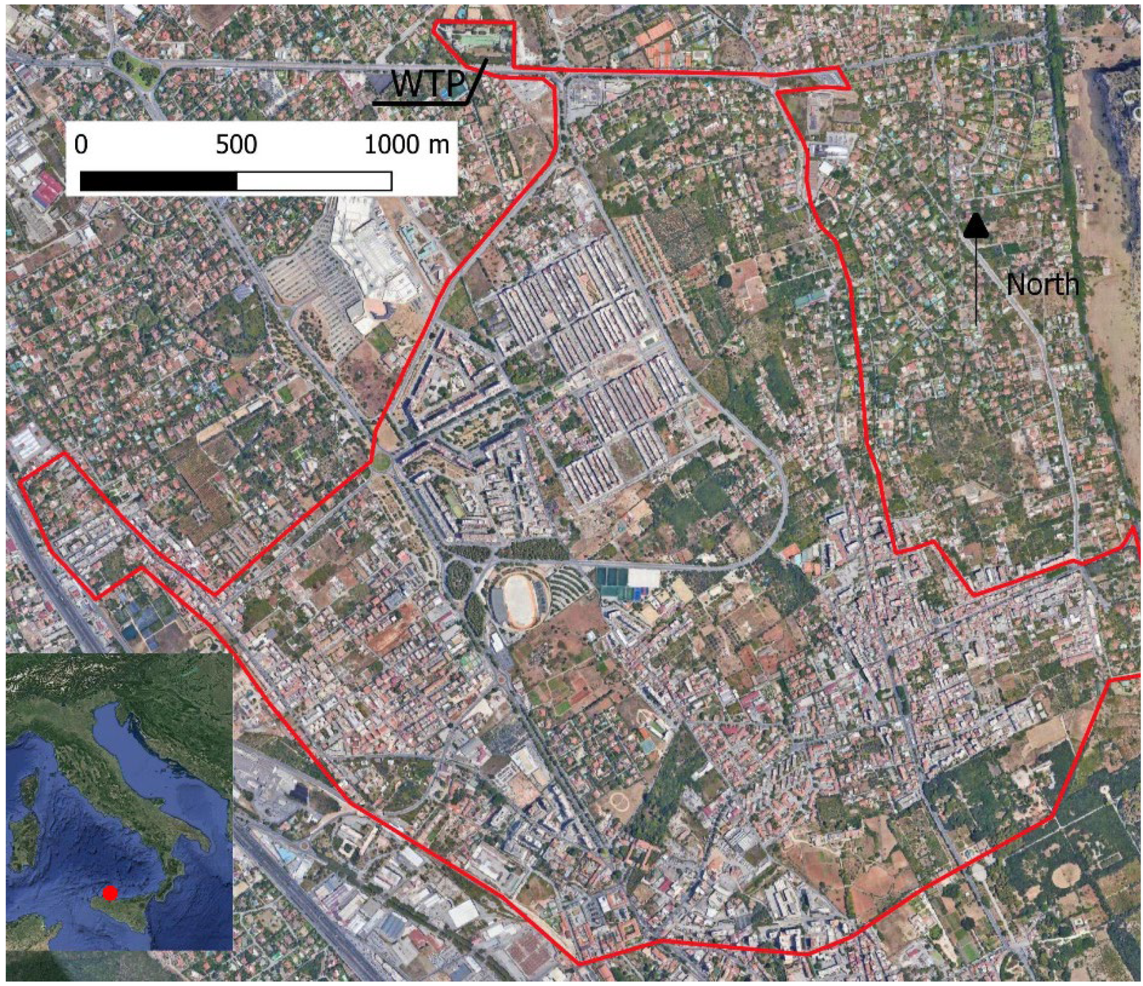
The case study is a district of the town of Palermo, called San Filippo Neri. A combined sewerage system collects wastewater and stormwater and conveys it to the Water Treatment Plant (WTP) called Fondo Verde (Figure 3).
The 2D computational domain has an extension of 4.958 km2 (Figure 3), and the entire surface is covered by a Digital Terrain Model (DTM) with a cell size of 2 m × 2 m. The sewer network has a circular (diameter from 0.30 m to 0.80 m) or egg-shaped cross-section (height from 0.50 m to 1.30 m). More than 400 gullies transfer part of the runoff from the roads to the sewer. The gullies, generally, have a square shape with gratings. Their interception length Lin can be grouped in three values (0.80, 1.00 and 1.20 m). The open area Ain changes from 0.080 to 0.180 m2. The upper 2D domain was discretized with a triangular unstructured mesh, composed of 83,328 elements and 42,715 nodes. The mesh was initialized using the open-source mesh generator NETGEN [46] and corrected with the algorithm presented in [20] to guarantee the generalized Delaunay property. The length of the triangle sides changes from 10 to 15 m. The sewer network is modeled with 4657 nodes, 4655 edges and 420 road gullies.
In the 2D domain there are three outlet sections, made up of a total of 6 mesh nodes (cyan arrows in Figure 4): at the WTP toward the west (paved road 7 m wide), at Via Venere toward the east (paved road 10 m wide), at Piazza Castelforte toward the north (paved road 11 m wide). In these nodes, a small water depth was set as boundary condition.
In the lower 1D domain there are two outlet nodes (black arrows in Figure 4): the first one is at the inlet of the WTP (circular pipe 0.450 m diameter), and the second one is inside the sewer of Via Castelforte (circular pipe 0.400 m diameter). In these nodes, the kinematic condition is obtained by setting the water depth gradient equal to zero. All the runoff entering the combined sewer of Via Castelforte leaves the computational domain through the same sewer pipe, continuing up to the final receptor downstream of Piazza Castelforte.
A large part of the 2D computational domain is covered by agricultural soils or gardens, with strong permeability. The total permeable area is 2.150 km2 (43% of the whole domain). These permeable areas are often bounded by low walls marking single properties (Figure 5). As a consequence, the runoff after soil saturation does not flow onto the external road but remains inside the property and finally infiltrates inside the soil. For this reason, in these properties we assume a runoff coefficient equal to zero. In the remaining impermeable area (roads, roofs, parking), we assume a runoff coefficient equal to 1. The rainfall data were assigned to all the nodes of the 2D domain as inlet source terms.
Every 10 min, a rain gauge with 0.2 mm accuracy measures the rainwater depth falling in the WTP area (Figure 5). The rain gauge is part of the sensor network of the Department of Engineering of the University of Palermo (http://idrologia.unipa.it accessed on 12 January 2022). From the sewerage network the flow arrives in reception tank of the pumping station at the WTP, where the water depths are measured by the AMAP SpA water company, the manager of the WTP.
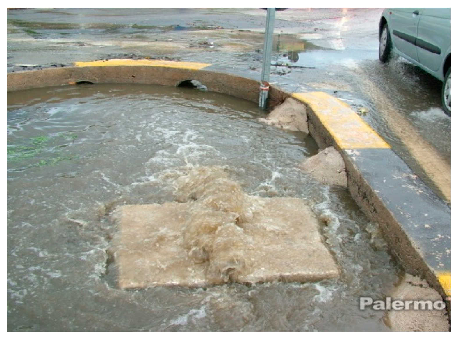
In September and October 2021 different rainfalls caused sewer surcharges and local flooding from manholes. In particular, on 11 September, and 1 and 10 October (Figure 6) local flooding from the manholes to the road at Piazza Castelforte occurred (Observation point 1—Figure 4 and Figure 7). The rainfall depth was respectively 8.4, 7.8 and 11.2 mm, corresponding to a rainfall duration of 80 min, 50 min and 4 h 40 min (Figure 6).
Other severe rains occurred on 2 and 5 October (Figure 8). In addition to local flooding at Piazza Castelforte, additional local flooding from the reception tank to the paved area at WTP occurred (Observation point 2—Figure 4 and Figure 9). The two corresponding rains were 43.0 and 15.4 mm, respectively, corresponding to a rainfall duration of 1 h 50 min, and 2 h 30 min (Figure 8). The sewer flow entering the WTP during the aforementioned events achieved a maximum value of 0.05 m3/s against a total flow of about 0.740 m3/s in the inlet pipe and has been neglected.
The two events with local flooding only at Piazza Castelforte occurring on 1 and 10 October (rains 7.8 and 11.2 mm) were used for calibration. The other three events were used for validation (Table 1). We assume the roughness uncertainty to be much smaller in the sewer pipes than in the ground surface of the 2D domain. On the basis of this assumption, we assigned to the sewer pipes a Manning coefficient np equal to 0.020 m−1/3s. The parameter of the calibration is only the Manning’s roughness ns of the 2D domain inside the impermeable areas. The Manning’s tested value ranged from ns = 0.018 m−1/3s to ns = 0.024 m−1/3s.
In the range ns = 0.020 and ns = 0.022 m−1/3s, during the two calibration events, sewer surcharging with overflow only occurred at Piazza Castelforte (green point in Figure 10). Surcharging in the sewer branches close to the WTP is also simulated (blue lines); in most of the sewer branches open flow conditions held during all the event (green lines). In the upper 2D, domain the computed water depths always remained lower than 0.20 m (water depths from 0.05 and 0.20 m cyan color; water depths lower than 0.05 m white color). Figure 10 shows the sewer filling degree (Depth/Diameter ratio) and the water depth in the 2D domain calculated by the numerical simulation.
In the two calibration events, for ns < 0.018 m−1/3s, at Piazza Castelforte storm overflow from the manhole is missing. For ns > 0.024 m−1/3s sewer surcharging with a local overflow at the WTP occurred, in addition to the one in Piazza Castelforte.
Table 2 shows a summary of the qualitative information used for calibration and a measure of the similarity S of the qualitative observation with the computed data, for each trial value of the Manning coefficient. The similarity S was computed by summing 1/n for each positive match, −1/n for each negative match, 0 for each missing comparison, where n is the number of events (2 for calibration and 3 for validation). According to Table 2, an optimal ns = 0.021 m−1/3s has been selected.
In the first validation event (11 September 2021, rain 8.4 mm), the results were similar to those obtained during calibration (Figure 11). The extension of the computed surcharging pipes (blue lines) was smaller than those used previously. A local overflow occurred at Piazza Castelforte according to local interviews.
In the second validation event (5 October, rain 15.4 mm) a local overflow occurred at both WTP and Piazza Castelforte (Figure 12), according to local interviews. In addition to the local overflow at WTP and Piazza Castelforte, three other simulated manholes created local flooding (green points in Figure 12), but direct observations are missing. In the 2D upper domain, water depths between 0.20 and 0.50 m were simulated.
On 2 October 2021, the measured rainfall was 43.0 mm in two hours. The simulation reproduccing the sewer overflow registered at both the WTP and Piazza Castelforte (green points in Figure 13). The local flooding from manholes was also simulated in many other manholes; we know that surcharging affected different reaches of the sewers, but direct observations are missing. In different areas of the upper domain water depths between 0.20 and 0.50 m were simulated. In Figure 13, a picture shows the flooded urban area, with a water depth of about 20 cm, consistent with the mean value computed by the model.
See in Table 3 the similarities computed for the validation events with the calibrated Manning coefficient ns = 0.021.
Finally, a sensitivity analysis has been carried out for the selected Manning coeffi-cient np of the sewer pipes. Results obtained using the optimal ns of the 2D domain and a np value in the range 0.018 < np < 0.022 provide the same similarity values, and a more ac-curate estimation of this parameter is not possible from the available information.
All simulations were carried out with a single 11th Gen Intel® CORE(TM) i5-1135G7 CPU processor at 2.40 GHz assuming a time step equal to 20 s. The computational CPU times were between 9 and 17 min. Table 4 shows details of the computational CPU time obtained for each event.
4. Discussion
The proposed EWEC model has the ambition of being a useful tool for the urban flood simulations in the context of hydraulic risk mapping. A major advantage of the model is the stability of its results with respect to the time step size, as well as to the uncertainty in the estimated topographic levels and in the selected Manning coefficient [21]. This uncertainty is due, along with the general lack of available measures, also to the spatial discretization associated with the local meshing, to the small scale variability of the physical parameters and to the seasonal variation of the vegetation. In [20] it is shown that, for the solution of a simple test computing the flood from a single straight channel inside a flat area, the diffusive model attains almost the same results as the complete one even using a very low mesh density, while the results of the complete one strongly depends on the selected mesh density up to a very high sill value.
The stability of the computed results with respect to the Manning coefficient allows the use of a simple zonation and the selection of several parameters for the model calibration. In the study case, only “qualitative” measures were available for both the calibration and the validation events, including possible surcharging occurring in two gullies. However, the results obtained with the calibration of a single parameter are fully consistent with mean water levels observed in the area according to the available pictures within a large interval of physically consistent Manning values. Mesh density analysis, not documented here for sake of simplicity, shows also a general stability of the results, and the density of the unstructured triangular mesh has been selected only on the basis of the predicted water level and velocity heterogeneity.
The advantages of the original WEC model are saved, in the new dual 2D-1D EWEC model, thanks to the fully coupled solution of the two layers, physically connected through the vertical manholes. To guarantee the same stability obtained in the solution of the two single layers, we need to solve linear systems that have an order equal to the total number of unknowns. This number is equal to the sum of the nodes of the 2D mesh plus the number of the computational cells of the 1D domain, but the system matrix is well-conditioned and allows, for a single event of several ours, a quick solution even with hundreds of thousands of computational cells and the use of a simple one-processor PC.
Parallel computing can be easily applied only to the correction step of the MAST algorithm solving the equation system (1)–(6). Parallel solution of the prediction problem in 2D and 3D domains is possible but requires a specific coding which is in progress at present time.
5. Conclusions
The EWEC model, for urban flood simulations, has been presented, along with its novelty and limitations. The main novelty of the model is the fully coupled solution of the upper 2D and the lower 1D sewer domains, with the 2D domain discretized with an un-structured triangular mesh. Application to a real event which occurred in a small basin area has shown the robustness of the model, been calibrated against “qualitative” data using only one parameter.
Author Contributions
Conceptualization, T.T. and C.N.; methodology, M.S. and T.T.; software, M.S. and T.T.; validation, C.N.; formal analysis, C.N. and T.T.; data curation, C.N. and M.S.; writing—original draft preparation, T.T., C.N. and M.S.; writing—review and editing, T.T., C.N. and M.S.; visualization, M.S. and C.N.; supervision, T.T.; All authors have read and agreed to the published version of the manuscript.
Funding
This research received no external funding.
Acknowledgments
The authors thank engineer Sergio Agati of the AMAP company for providing the water depth data at the reception tank of the Fondo Verde water treatment plant.
Conflicts of Interest
The authors declare no conflict of interest.
References
- Shah, M.A.R.; Rahman, A.; Chowdhury, S.H. Challenges for achieving sustainable flood risk management. J. Flood Risk Manag. 2018, 11, S352–S358. [Google Scholar] [CrossRef] [Green Version]
- Meyer, V.; Priest, S.; Kuhlicke, C. Economic evaluation of structural and non-structural flood risk management measures: Examples from the Mulde River. Nat. Hazards 2012, 62, 301–324. [Google Scholar] [CrossRef]
- White, I.; Connelly, A.; Garvin, S.; Lawson, N.; O’Hare, P. Flood resilience technology in Europe: Identifying barriers and co-producing best practice. J. Flood Risk Manag. 2018, 11, S468–S478. [Google Scholar] [CrossRef]
- Kumar, P.; Debele, S.E.; Sahani, J.; Aragão, L.; Barisani, F.; Basu, B.; Bucchignani, E.; Charizopoulos, N.; Di Sabatino, S.; Domeneghetti, A.; et al. Towards an operationalisation of nature-based solutions for natural hazards. Sci. Total Environ. 2020, 731, 138855. [Google Scholar] [CrossRef]
- Blázquez, L.; García, J.A.; Bodoque, J.M. Stakeholder analysis: Mapping the river networks for integrated flood risk management. Environ. Sci. Policy 2021, 124, 506–516. [Google Scholar] [CrossRef]
- Tobin, G.A. The levee love affair: A stormy relationship? J. Am. Water Resour. Assoc. 1995, 31, 359–367. [Google Scholar] [CrossRef]
- Teng, J.; Jakeman, A.J.; Vaze, J.; Croke, B.F.W.; Dutta, D.; Kim, S. Flood inundation modelling: A review of methods, recent advances and uncertainty analysis. Environ. Model. Softw. 2017, 90, 201–216. [Google Scholar] [CrossRef]
- Castellarin, A.; Domeneghetti, A.; Brath, A. Identifying robust large-scale flood risk mitigation strategies: A quasi-2D hydraulic model as a tool for the Po river. Phys. Chem. Earth 2011, 36, 299–308. [Google Scholar] [CrossRef]
- Moussa, R.; Bocquillon, C. On the use of the diffusive wave for modelling extreme flood events with overbank flow in the floodplain. J. Hydrol. 2009, 374, 116–135. [Google Scholar] [CrossRef]
- Morales-Hernández, M.; Murillo, J.; Lacasta, A.; Brufau, P.; García-Navarro, P. A Conservative Strategy to Couple 1D and 2D Numerical Models: Application to Flooding Simulations. In Proceedings of the International Conference on Fluvial Hydraulics, Lausanne, Switzerland, 3–5 September 2014. [Google Scholar]
- Villanueva, I.; Wright, N.G. Performance of Several Hybrid Numerical Schemes to Determine Flooding Extent. In Proceedings of the International Conference on Fluvial Hydraulics, St. Louis, MI, USA, 10–14 July 2016. [Google Scholar]
- Aricò, C.; Filianoti, P.; Sinagra, M.; Tucciarelli, T. The FLO diffusive 1D-2D model for simulation of river flooding. Water 2016, 8, 200. [Google Scholar] [CrossRef]
- Bates, P.D.; Horritt, M.S.; Fewtrell, T.J. A simple inertial formulation of the shallow water equations for efficient two-dimensional flood inundation modelling. J. Hydrol. 2010, 387, 33–45. [Google Scholar] [CrossRef]
- Ponce, V.M. Generalized diffusion wave equation with inertial effects. Water Resour. Res. 1990, 26, 1099–1101. [Google Scholar] [CrossRef]
- Costabile, P.; Costanzo, C.; Macchione, F. Performances and limitations of the diffusive approximation of the 2-d shallow water equations for flood simulation in urban and rural areas. Appl. Numer. Math. 2016, 116, 141–156. [Google Scholar] [CrossRef]
- Tsai, C.W. Applicability of kinematic, noninertia, and quasi-steady dynamic wave models to unsteady flow routing. J. Hydraul. Eng. 2003, 129, 613–627. [Google Scholar] [CrossRef]
- Di Cristo, C.; Iervolino, M.; Vacca, A. Applicability of kinematic, diffusion, and quasi-steady dynamic wave models to shallow mud flows. J. Hydrol. Eng. 2014, 19, 956–965. [Google Scholar] [CrossRef]
- Cea, L.; Garrido, M.; Puertas, J. Experimental validation of two-dimensional depth-averaged models for forecasting rainfall-runoff from precipitation data in urban areas. J. Hydrol. 2010, 382, 88–102. [Google Scholar] [CrossRef]
- Schubert, J.E.; Sanders, B.F.; Smith, M.J.; Wright, N.G. Unstructured mesh generation and landcover-based resistance for hydrodynamic modeling of urban flooding. Adv. Water Resour. 2008, 31, 1603–1621. [Google Scholar] [CrossRef]
- Aricò, C.; Sinagra, M.; Begnudelli, L.; Tucciarelli, T. MAST-2D diffusive model for flood prediction on domains with triangular Delaunay unstructured meshes. Adv. Water Resour. 2011, 34, 1427–1449. [Google Scholar] [CrossRef] [Green Version]
- Guinot, V.; Cappeleare, B. Sensitivity analysis of 2D steady-state shallow water flow. Application to free surface model calibration. Adv. Water Resour. 2009, 32, 540–560. [Google Scholar] [CrossRef]
- Spada, E.; Sinagra, M.; Tucciarelli, T.; Biondi, D. Unsteady state water level analysis for discharge hydrograph estimation in rivers with torrential regime: The case study of the February 2016 flood event in the Crati River, South Italy. Water 2017, 9, 288. [Google Scholar] [CrossRef]
- Wu, T.; Li, J.; Li, T.; Sivakumar, B.; Zhang, G.; Wang, G. High-efficient extraction of drainage networks from digital elevation models constrained by enhanced flow enforcement from known river maps. Geomorphology 2019, 340, 184–201. [Google Scholar] [CrossRef]
- Nasello, C.; Tucciarelli, T. Dual multilevel urban drainage model. J. Hydraul. Eng. 2005, 131, 748–754. [Google Scholar] [CrossRef]
- Leandro, J.; Chen, A.S.; Djordjevi´c, S.; Savi´c, D.A. Comparison of 1D/1D and 1D/2D Coupled (Sewer/Surface) Hydraulic Models for Urban Flood Simulation. J. Hydraul. Eng. 2009, 135, 495–504. [Google Scholar] [CrossRef]
- He, J.; Qiang, Y.; Luo, H.; Zhou, S.; Zhang, L. A stress test of urban system flooding upon extreme rainstorms in Hong Kong. J. Hydrol. 2021, 597, 125713. [Google Scholar] [CrossRef]
- Zhang, H.; Wu, W.; Hu, C.; Hu, C.; Li, M.; Hao, X.; Liu, S. A distributed hydrodynamic model for urban storm flood risk assessment. J. Hydrol. 2021, 600, 126513. [Google Scholar] [CrossRef]
- Li, Q.; Liang, Q.; Xia, X. A novel 1D-2D coupled model for hydrodynamic simulation of flows in drainage networks. Adv. Water Resour. 2020, 137, 103519. [Google Scholar] [CrossRef]
- Sañudo, E.; Cea, L.; Puertas, J. Modelling pluvial flooding in urban areas coupling the models iber and SWMM. Water 2020, 12, 2647. [Google Scholar] [CrossRef]
- Glenis, V.; McGough, A.S.; Kutija, V.; Kilsby, C.; Woodman, S. Flood modelling for cities using Cloud computing. J. Cloud Comput. 2013, 2, 7. [Google Scholar] [CrossRef] [Green Version]
- Cea, L.; Garrido, M.; Puertas, J.; Jácome, A.; Del Río, H.; Suárez, J. Overland flow computations in urban and industrial catchments from direct precipitation data using a two-dimensional shallow water model. Water Sci. Technol. 2010, 62, 1998–2008. [Google Scholar] [CrossRef]
- Chang, T.J.; Wang, C.H.; Chen, A.S.; Djordjevi´c, S. The effect of inclusion of inlets in dual drainage modelling. J. Hydrol. 2018, 559, 541–555. [Google Scholar] [CrossRef]
- Fernández-Pato, J.; García-Navarro, P. An efficient gpu implementation of a coupled overland-sewer hydraulic model with pollutant transport. Hydrology 2021, 8, 146. [Google Scholar] [CrossRef]
- Dong, X.; Guo, H.; Zeng, S. Enhancing future resilience in urban drainage system: Green versus grey infrastructure. Water Res. 2017, 124, 280–289. [Google Scholar] [CrossRef]
- Kim, S.E.; Lee, S.; Kim, D.; Song, C.G. Stormwater Inundation Analysis in Small and Medium Cities for the Climate Change Using EPA-SWMM and HDM-2D. J. Coast. Res. 2018, 85, 991–995. [Google Scholar] [CrossRef]
- Qiang, Y.; Zhang, L.; He, J.; Xiao, T.; Huang, H.; Wang, H. Urban flood analysis for Pearl River Delta cities using an equivalent drainage method upon combined rainfall-high tide-storm surge events. J. Hydrol. 2021, 597, 126293. [Google Scholar] [CrossRef]
- Palla, A.; Colli, M.; Candela, A.; Aronica, G.T.; Lanza, L.G. Pluvial flooding in urban areas: The role of surface drainage efficiency. J. Flood Risk Manag. 2018, 11, S663–S676. [Google Scholar] [CrossRef]
- Guerreiro, S.B.; Glenis, V.; Dawson, R.J.; Kilsby, C. Pluvial flooding in European cities-A continental approach to urban flood modelling. Water 2017, 9, 296. [Google Scholar] [CrossRef] [Green Version]
- Sinagra, M.; Nasello, C.; Tucciarelli, T.; Barbetta, S.; Massari, C.; Moramarco, T. A Self-Contained and Automated Method for Flood Hazard Maps Prediction in Urban Areas. Water 2020, 12, 1266. [Google Scholar] [CrossRef]
- Francipane, A.; Pumo, D.; Sinagra, M.; la Loggia, G.; Noto, L.V. A paradigm of extreme rainfall pluvial floods in complex urban areas: The flood event of 15 July 2020 in Palermo (Italy). Nat. Hazards Earth Syst. Sci. 2021, 21, 2563–2580. [Google Scholar] [CrossRef]
- Filianoti, P.; Gurnari, L.; Zema, D.A.; Bombino, G.; Sinagra, M.; Tucciarelli, T. An Evaluation Matrix to Compare Computer Hydrological Models for Flood Predictions. Hydrology 2020, 7, 42. [Google Scholar] [CrossRef]
- Henderson, F.M. Open Channel Flow; Pearson College Div: New York City, NY, USA, 1996. [Google Scholar]
- Spada, E.; Tucciarelli, T.; Sinagra, M.; Sammartano, V.; Corato, G. Computation of vertically averaged velocities in irregular sections of straight channels. Hydrol. Earth Syst. Sci. 2015, 19, 3857–3873. [Google Scholar] [CrossRef]
- Aricò, C.; Tucciarelli, T. A marching in space and time (MAST) solver of the shallow water equations. Part I: The 1D model. Adv. Water Resour. 2017, 30, 1236–1252. [Google Scholar] [CrossRef]
- Noto, L.; Tucciarelli, T. DORA algorithm for network flow models with improved stability and convergence properties. J. Hydraul. Eng. 2001, 127, 380–391. [Google Scholar] [CrossRef]
- Schöberl, J. NETGEN—An advancing front 2D/3D-mesh generator based on abstract rules. Comput. Visualiz. Sci. 1997, 1, 41–52. [Google Scholar] [CrossRef] [Green Version]
Figure 1.
1D-2D computational grids coupling.

Figure 2.
Water depths and possible flow configurations inside manholes: (a) Flow to the sewer pipe in case of not fully submerged manhole condition; (b) Flow to the sewer pipe in case of fully submerged manhole condition; (c) Flow from the sewer pipe in case of fully submerged manhole condition.
Figure 2.
Water depths and possible flow configurations inside manholes: (a) Flow to the sewer pipe in case of not fully submerged manhole condition; (b) Flow to the sewer pipe in case of fully submerged manhole condition; (c) Flow from the sewer pipe in case of fully submerged manhole condition.

Figure 3.
Satellite view of 2D case study boundary outline.

Figure 4.
1D sewer network (black lines) and gullies (black points).

Figure 5.
Permeable soils inside the computational domain (left). Street view (Google) of boundary walls of permeable soil (right).
Figure 5.
Permeable soils inside the computational domain (left). Street view (Google) of boundary walls of permeable soil (right).

Figure 6.
Rainfall depth: events on 11 September, 1 October and 10 October 2021.

Figure 7.
Manhole overflow at Piazza Castelforte. Source: web (www.palermotoday.it accessed on 27 October 2021).
Figure 7.
Manhole overflow at Piazza Castelforte. Source: web (www.palermotoday.it accessed on 27 October 2021).

Figure 8.
Rainfall depth: events on 2 October and 5 October 2021.

Figure 9.
Overflow of the reception tank at the Water Treatment Plant.

Figure 10.
Results of event of 1 October 2021 (rain 7.8 mm). Part-full pipe flow (green line) and surcharging pipe (blue lines). The green point indicates the local overflow at Piazza Castelforte.
Figure 10.
Results of event of 1 October 2021 (rain 7.8 mm). Part-full pipe flow (green line) and surcharging pipe (blue lines). The green point indicates the local overflow at Piazza Castelforte.

Figure 11.
Results of validation event on 11 September 2021 (rain 8.4 mm). Part-full pipe flow (green lines) and surcharging pipe (blue lines). The green point indicates the local overflow at Piazza Castelforte.
Figure 11.
Results of validation event on 11 September 2021 (rain 8.4 mm). Part-full pipe flow (green lines) and surcharging pipe (blue lines). The green point indicates the local overflow at Piazza Castelforte.

Figure 12.
Results of validation event on 5 October 2021 (rain 15.4 mm). Part-full pipe flow (green lines) and surcharging pipe (blue lines). The green point indicates the local overflow at Piazza Castelforte and at WTP.
Figure 12.
Results of validation event on 5 October 2021 (rain 15.4 mm). Part-full pipe flow (green lines) and surcharging pipe (blue lines). The green point indicates the local overflow at Piazza Castelforte and at WTP.

Figure 13.
Results of validation event of 2 October 2021 (rain 43.0 mm). Part-full pipe flow (green lines) and surcharging pipe (blue lines). The green point indicates the local overflow at Piazza Castelforte, at the WTP and in other streets.
Figure 13.
Results of validation event of 2 October 2021 (rain 43.0 mm). Part-full pipe flow (green lines) and surcharging pipe (blue lines). The green point indicates the local overflow at Piazza Castelforte, at the WTP and in other streets.


Table 1.
Characteristics of rainfall events.
| Event | Event ID | Rainfall Depth (mm) | Rainfall Duration (Hours:Minutes) | Max Rainfall Intensity (mm/h) | Use in the Model |
|---|---|---|---|---|---|
| 11 September 2021 | VE1 | 8.4 | 1:10 | 18.0 | Validation |
| 1 October 2021 | CE2 | 7.8 | 0:50 | 26.4 | Calibration |
| 2 October 2021 | VE3 | 43.0 | 1:50 | 109.2 | Validation |
| 5 October 2021 | VE4 | 15.4 | 2:30 | 60.0 | Validation |
| 10 October 2021 | CE5 | 11.2 | 4:40 | 15.6 | Calibration |
Table 2.
Calibration similarity matrix.
| Surcharge in Piazza Castelforte | Flooding WTP | Similarity | |||
|---|---|---|---|---|---|
| Manning [m−1/3s]\event | CE2 | CE5 | CE2 | CE5 | - |
| 0.018 |  | | | | 0.0 |
| 0.020 |  | | | | 2.0 |
| 0.022 | | | | | 2.0 |
| 0.024 | | | | | 0.0 |
| Observed | | | | | - |
Table 3.
Validation similarity matrix.
| Surcharge in Piazza Castelforte | Flooding WTP | Similarity | |||||
|---|---|---|---|---|---|---|---|
| Manning [m−1/3s]\event | VE1 | VE3 | VE4 | VE1 | VE3 | VE4 | - |
| 0.021 | | | | | | | 2.0 |
| Observed | | | | | | | - |
Table 4.
Computational CPU times.
| Event | Rainfall Duration (Hours:Minutes) | CPU Time (Minutes) |
|---|---|---|
| 11 September 2021 | 1:10 | 10 |
| 1 October 2021 | 0:50 | 9 |
| 2 October 2021 | 1:50 | 17 |
| 5 October 2021 | 2:30 | 12 |
| 10 October 2021 | 4:40 | 15 |
Publisher’s Note: MDPI stays neutral with regard to jurisdictional claims in published maps and institutional affiliations. |
© 2022 by the authors. Licensee MDPI, Basel, Switzerland. This article is an open access article distributed under the terms and conditions of the Creative Commons Attribution (CC BY) license (https://creativecommons.org/licenses/by/4.0/).
Share and Cite
MDPI and ACS Style
Sinagra, M.; Nasello, C.; Tucciarelli, T. Urban Flood Prediction through GIS-Based Dual-Coupled Hydraulic Models. Hydrology 2022, 9, 174. https://0-doi-org.brum.beds.ac.uk/10.3390/hydrology9100174
AMA Style
Sinagra M, Nasello C, Tucciarelli T. Urban Flood Prediction through GIS-Based Dual-Coupled Hydraulic Models. Hydrology. 2022; 9(10):174. https://0-doi-org.brum.beds.ac.uk/10.3390/hydrology9100174
Chicago/Turabian StyleSinagra, Marco, Carmelo Nasello, and Tullio Tucciarelli. 2022. "Urban Flood Prediction through GIS-Based Dual-Coupled Hydraulic Models" Hydrology 9, no. 10: 174. https://0-doi-org.brum.beds.ac.uk/10.3390/hydrology9100174
Note that from the first issue of 2016, this journal uses article numbers instead of page numbers. See further details here.