
Provision of Desalinated Irrigation Water by the Desalination of Groundwater Abstracted from a Saline Aquifer


DCA Consultants Ltd., The Bungalow, Castleton Farm, Falkirk, Stirlingshire FK2 8SD, UK
Hydrology 2022, 9(7), 128; https://0-doi-org.brum.beds.ac.uk/10.3390/hydrology9070128
Submission received: 22 June 2022
/
Revised: 12 July 2022
/
Accepted: 19 July 2022
/
Published: 21 July 2022
(This article belongs to the Special Issue Groundwater Management)
Abstract
:Globally, about 54 million ha of cropland are irrigated with saline water. Globally, the soils associated with about 1 billion ha are affected by salinization. A small decrease in irrigation water salinity (and soil salinity) can result in a disproportionally large increase in crop yield. This study uses a zero-valent iron desalination reactor to effect surface processing of ground water, obtained from an aquifer, to partially desalinate the water. The product water can be used for irrigation, or it can be reinjected into a saline aquifer, to dilute the aquifer water salinity (as part of an aquifer water quality management program), or it can be injected as low-salinity water into an aquifer to provide a recharge barrier to protect against seawater intrusion. The saline water used in this study is processed in a batch flow, bubble column, static bed, diffusion reactor train (0.24 m3), with a processing capacity of 1.7–1.9 m3 d−1 and a processing duration of 3 h. The reactor contained 0.4 kg Fe0. A total of 70 batches of saline water (average 6.9 g NaCl L−1; range: 2.66 to 30.5 g NaCl L−1) were processed sequentially using a single Fe0 charge, without loss of activity. The average desalination was 24.5%. The reactor used a catalytic pressure swing adsorption–desorption process. The trial results were analysed with respect to Na+ ion removal, Cl− ion removal, and the impact of adding trains. The reactor train was then repurposed, using n-Fe0 and emulsified m-Fe0, to establish the impact of reducing particle size on the amount of desalination, and the amount of n-Fe0 required to achieve a specific desalination level.
1. Introduction
Over the last two decades, irrigation has accounted for about 70% of global anthropogenic water usage from freshwater [1,2,3,4]. It accounts for 90% of anthropogenic consumptive water usage [1,3]. About 40% of freshwater withdrawals are from groundwater [1]. About 66% of the global population lives under water stress conditions [4]. The global agricultural land area is about 5 billion ha, of which about 1.24 billion ha is arable cropland [5]. Since 2000, the global cropland area has expanded by about 10% [5]. The global distribution of cropland and associated soil types are discussed elsewhere [5,6].
There is a clear link between global food availability and global poverty [7]. It is estimated that a 1% increase in global food production could result in a 0.48% decline in global poverty [7]. Since 1850, global cropland has increased from about 5% of global land area to about 10% of global land area [8]. Over the same time period, the proportion of global land used to rear livestock has increased from about 10% to about 25% of the global land area [8].
Between 1850 and 2014, the area of cropland, which is subject to irrigation, has risen exponentially, from about 28 million ha in 1850 to about 270 million ha in 2014 [8]. A regression analysis of the published [8] irrigated cropland area vs. year data for 1850 to 2014 indicates the following:
Irrigated cropland area, million ha = 0.0000000001e0.0144778779[Year], R2 = 98.67%.
Extrapolation of this trend to 2050 indicates that the global irrigated area could potentially expand from 270 million ha in 2014 to >700 million ha by 2050. Irrigated cropland currently accounts for around 40% of global food production [9,10]. More than 1 billion ha of land is negatively affected by salinization, including about 20% of the global irrigated cropland (54 million ha) [11]. About 34 million ha of salinized land has become salinized as a direct result of irrigation [11]. Globally, about 424 million ha of topsoil (0–30 cm) and 833 million ha of subsoil (30–100 cm) are salinized [11]. The term salinized is used to refer to soil or water with an electrical conductivity of >4 dSm−1 (mScm−1) [11]. The potential future global cropland land resource in areas where the soil is salinized is estimated at >200 million ha [11].
Global food demand is expected to rise by between 60% and 100% by 2050 [9,10]. This rise in food demand results from the expected increase in global population from 7.7 billion in 2017 [11] to 9.1 billion people in 2050 [9,10], and 11.2 billion by 2100 [11]. The majority of the future increase in food production required to meet this demand will be confined to areas that are salinized or are currently irrigated with saline water or become newly irrigated with saline water.
Irrigated water demand is <5000 m3 ha−1 a−1 for most greenhouses, 1000–10,000 m3 ha−1 a−1 for most arable crops, and >50,000 m3 ha−1 a−1 for some rice crops. The use of saline irrigation water adversely affects crop yields [12,13], crop diversity [12], crop value, soil quality [11], local groundwater quality, local riparian systems, local groundwater levels, and land use.
Desalination, partial desalination, freshwater dilution, additional processing, or treatment of this saline irrigation water has the potential to substantially increase crop yields, increase crop varieties, and increase crop quality and value, while improving soil quality, groundwater quality, and riparian water quality. The process flow adopted in this study to assist in raising the yields of crops currently irrigated with saline water is summarized in Figure 1.
Saline irrigation, when compared with freshwater irrigation, results in reduced crop yields (t ha−1) and reduced crop value (USD t−1). It reduces the number of alternative crops that can be grown on an agricultural unit and results in increased soil salinization. Irrigated crops have a low sale price (USD t−1, USD ha−1), a high fixed operating cost (USD ha−1), and a low variable operating cost (USD ha−1). Irrigating with desalinated, or partially desalinated, water increases the sale price (USD ha−1) and increases the variable operating cost (USD ha−1). The viability of irrigation with desalinated water, or partially desalinated water, is a function of the interaction between crop sale price, crop yield, and increased operating costs.
The various desalination processes are summarized in Appendix A. About 100 million m3 d−1 of water is desalinated, of which about 60% is derived from seawater [14]. Most of this desalinated water is used to provide potable and municipal water. It is typically produced for a cost of >USD 3.5 m−3, using either reverse osmosis (RO) or thermal evaporation (Appendix A, Figure A1). These processes produce potable water and a reject brine containing the removed NaCl. The use of desalinated water for irrigation is not economically viable in most areas, and for most crops, due to its high cost and environmental issues associated with the disposal of the reject brine. Another option may be to use partially desalinated water, produced by a passive chemical process (Appendix A, Figure A2), such as zero-valent iron (ZVI, Fe0) desalination. This process produces partially desalinated water with no reject brine waste product.
1.1. Zero-Valent Iron Desalination
This study, considers, whether it is possible, to use zero-valent iron (ZVI, Fe0) desalination, to partially desalinate groundwater, or seawater. The product water may be suitable for irrigation, or for injection, into a saline aquifer to reduce its salinity, or for injection into an aquifer, which is affected by seawater incursion to form a recharge barrier.
Zero-valent iron desalination (Appendix A, Figure A3) was first discovered [15] in 2010. The discoveries used a continuously stirred reactor (CSR) [15,16] and a diffusion reactor. Since then, ZVI desalination has been verified in a variety of reactor types, in different patents, and publications (Appendix A, Figure A3). ZVI desalination can occur in fixed bed reactors, operating with a very slow water flow rate, for example, a permeable reactive barrier (PRB).
In each example (Appendix A, Figure A3), the feed water [A] had a salinity [y], and the product water [B] had a salinity [x], where 0 < [x] < [y].
ZVI currently costs between USD 200/t and USD 100,000/t (FOB). In order to be potentially economically viable for the partial desalination of irrigation water, the volume of water processed must be substantially in excess of 10,000 m3 t−1 Fe0. This will enable the process to produce a finished product cost within the range USD 0.05 m−3–USD 1.5 m−3.
The amount of desalination associated with ZVI varies with each water batch processed. This variability reflects the chemical nature of the process. Any commercial application of the technology for irrigation will require to use a desalination plant containing multiple reactor trains, operating in parallel. These trains will discharge water to a holding tank, mixing tank, reservoir, or aquifer.
1.2. Study Objectives
This study investigates whether a batch flow, bubble column, static bed, diffusion reactor (Appendix A, Figure A3), could be used, to provide partially desalinated water, for irrigation, or water injection.
A scalable, single reactor train was constructed (Figure 2), with the capability of processing 1.7 to 1.9 m3 d−1. The design concept envisaged a commercial scale up to a unit producing 170 to 340 m3 d−1. This would require 100 to 200 reactors operating in parallel.
In a commercial unit this would create a reactor footprint of between 20 and 40 m2. The commercial unit would require an air compressor capable of delivering 100 to 200 L m−1. The reactors would contain 50–100 kg Fe0 held in disposable cartridges. The plant would have 500–1000 m3 of feed water and product water storage tanks.
The commercial viability of this process requires:
- A single ZVI charge to be able to process multiple batches (or volumes) of water without loss of activity. Commercial ZVI water remediation plants, removing dissolved organic matter (DOM), organic solutes, and metals have demonstrated:
- ○
- >3.8 million m3 water processed t−1 Fe0 to remove DOM in a 22,500 m3 d−1 reactor [17].
- ○
- >24,000 m3 water processed t−1Fe0 to remove organic matter in a 60,000 m3 d−1 reactor [17].
- ○
- >466 m3 water processed t−1 Fe0 to remove arsenic in a 9.6 m3 d−1 reactor [17].
- ○
- >17,356 m3 water processed t−1 Fe0 to remove arsenic in a 5.2 m3 d−1 reactor [17].
- ○
- >2500 m3 water processed t−1 Fe0 to remove gold in a 30 m3 d−1 reactor [17].
To date, a single ZVI charge in an experimental ZVI desalination reactor has not been able to process >14,000 m3 water t−1 Fe0. One of the objectives of this study is to determine if the amount of water that can be processed by ZVI, can be increased to >42,000 m3 water-processed t−1 Fe0 without a loss of desalination activity.
- A method or process to be established and incorporated in a plant, which allows the highly variable product outcome from each batch to be compensated for. Another of the objectives of this study is to assess the product outcome variability and determine how the product quality problems associated with this variability may be overcome in a future commercial unit.
- Consideration as to whether replacement of Fe0 [17] with emulsified n/m-Fe0 or with n-Fe0 will give a higher level of desalination and will allow the amount of Fe used to be decreased. Another of the objectives of this study is to assess whether Fe0 could be replaced by n-Fe0 in a future commercial unit.
This study contains two appendices, Appendix A, and Appendix B. Appendix A provides a summary of the different desalination approaches. Appendix B, Table A1 and Table A2, provide the systematic dataset used in this study.
2. Materials and Methods
2.1. Reactor
The reactor process flow used in this study is summarized in Figure 2. The reactor is filled from a saline water feed tank. Product water is discharged to a product water tank. A cartridge containing ZVI is placed in the reactor. An air compressor is used to pressurize and fill (20 L) a pressured (0.8 MPa) gas tank with air. Air contained in the gas tank is discharged through the reactor (Figure 2). The product air is vented into the atmosphere.
The batch reactor (Figure 2) was constructed using a tank with a u-PVC shell. It had a 0.45 m diameter and contained 240 L of saline water. The water column depth exceeded 1.5 m. An 8 mm O.D. Cu0 conduit connected the gas tank (Figure 2) to a brass gas distributer. The brass gas distributer was placed at the base of the batch reactor. A 4 cm diameter, 0.7 m long, open-ended ABS cartridge containing 0.4 kg of steel wool (Fe0) was placed in the reactor (Figure 3). The cartridge was placed within a cartridge holder (Figure 4). An air compressor was used to supply 60 L air h−1 to the saline water.
2.2. ZVI
2.2.1. Steel Wool
The steel wool was prepared prior to use by soaking the steel wool in 10 L of water containing FeSO4 and urea (1:2.5 by weight (7 g L−1)) for 24 h. The steel wool has a structural porosity of >80%. The 4 cm diameter, 0.7 m long ABS cartridges were structured with a high-permeability-filter wool plug at each end (Figure 3). Each cartridge was filled with 0.4 kg of drained pretreated steel wool.
The pretreatment resulted in the iron fibres developing an irregular surface and a thin organic Fe(OH)x coating.
2.2.2. m-Fe0
Trials RT1, RT2, and RT4 used m-Fe0 + m-Cu0 + m-Al0 powders. Particle size was 0.002 to 0.08 mm. The zero-valent metals were purchased from MB Fiberglass, Newtownabbey, UK. Photomicrographs of these powders are provided in Reference [18].
2.2.3. Zero-Valent Iron Characterization
All catalytic reactants have an inherent reactivity that can be defined in terms of an intrinsic forward rate constant, kins. This intrinsic rate constant (change per unit time) is normally standardized in batch ZVI studies to a particle surface area (as) of 1 m2 g−1 and a particle concentration (Pw) of 1 g L−1. The observed forward rate constant (change s−1) in a batch flow (or continuous flow) reactor is then calculated [17,18] as
kobs = kins as Pw,
Over the last 30 years, the principal focus of catalytic and adsorption ZVI studies, in improving kobs has been to concentrate on reducing particle size and increasing particle shape irregularity to increase as. This has the effect of increasing the number of available catalytic and adsorption sites for a specific particle size.
The underlying assumptions are as follows:
- At any specific time, a proportion of the unoccupied sites will be available for either adsorption or catalytic activity.
- All catalytic and adsorption activity occurs at sites on the n-Fe0.
Laboratory catalyst and adsorbent studies, which have focused on this aspect of ZVI remediation, and are trying to develop a new form of n-Fe0, commonly use TEM, SEM-EDX, BET, XRD, XRF, microprobe, or similar analytical tools to define their product. They assume that kobs will increase if as increases.
Another group of laboratory studies have focused specifically on increasing the ability of a site to operate as a catalyst or adsorbent. These studies tend to focus on increasing the porosity of particles [17], mixing metal combinations [17,18], and controlling the dispersion of promoters on and within the particles [17]. Their specific objective is to increase kins [17,18].
Fe0, m-Fe0, and n-Fe0 are highly reactive in the presence of oxygen and water [17]. n-Fe0 is pyrophoric. Placement of Fe0, m-Fe0, and n-Fe0 in acidic water (pH ≤ 7) will result in the dissolution of the particles to release Fe2+ ions. In alkali water (pH = 7), the Fe0, m-Fe0, and n-Fe0 will initially be coated in white rust (Fe(OH)2) [17]. Further oxidation will result in the formation of green rust and various other iron oxyhydroxides [17].
Remediation studies, which seek to use Fe0, m-Fe0, and n-Fe, as an adsorbent or catalyst, will commonly pretreat the Fe0 to provide a surface coating to retard the formation of Fe2+ [17]. These coatings can also remove the pyrophoric characteristic of n-Fe0 and improve safety when handling this material [17].
Traditionally, steel wool is used to treat water by altering its Eh and pH, and thereby affects remediation by altering redox equilibria of pollutants. The release of Fe2+ ions has a side effect which results in the steel wool being an effective remediator of pollutants by coagulation. This results in both biota and pollutants being removed by the FexOyHz coagulants [19,20]. A number of pretreatment and characterization tools have been developed for steel wool [21]. Pretreatment does not enhance the reactivity of steel wool [21] but can reduce the rate of Fe2+ dissolution [22].
If, in this study, the steel wool was to be used to produce Fe2+ ions, then this could be characterized by measuring the rate of Fe2+ release. ZVI desalination is considered to be a catalytic process [17]. Therefore, the pretreatment, and catalyst placement in the reactor is designed to decrease the probability that Fe2+ ions produced by the steel wool are released into the main water body. The cartridge design used in this study is intended to ensure that the majority of any Fe2+ ions formed are retained in the catalyst cartridge.
There is no consensus on how ZVI should be characterized for specific water remediation studies. Examples of the different approaches taken by different research groups are provided in references [23,24].
Steel wool has a low as, and a very low catalytic kins for Na+ ion and Cl− ion removal. These two factors would appear (Equation (2)) to render steel wool as being unsuitable for use as a desalination catalyst. However, steel wool is widely available and has a low cost, typically in the range USD 200–1000 t−1. This compares with USD 10,000–100,000 t−1 for n-Fe0.
A typical characterization study of Fe using one or more of TEM, SEM-EDX, BET, XRD, or XRF may cost in the range USD 10,000–100,000. While this may serve a purpose in defining as in n-Fe0, it is not cost-effective for steel wool. If you purchase your steel wool from a supplier [A] at USD 200 t−1, there is no point in spending >USD 10,000 characterizing its morphology and chemistry to determine if it might be, say, 10% more effective than if the steel wool was purchased from a supplier [B] at USD 300 t−1 when placed in a specific reactor process.
2.2.4. ZVI Desalination Characteristics
Equation (2) indicates that increasing the residence time of the water in the reaction environment will increase kobs. In ZVI desalination reactors, this is achieved through the use of either a water recycle loop, where water is continually circulated through a fluidized n-Fe0 bed (e.g., US Patent US10919784B2), or a diffusion reaction environment, where water is continually circulated between a storage tank or reservoir and a reaction area containing a static ZVI bed (e.g., UK Patent GB 2520775A), or the use of long reaction times (e.g., US Patent US10919784B2; UK Patent GB 2520775A).
In a fixed bed or fluidized bed reactor, increasing Pw will increase the water residence time within the reaction environment for a specific water flow rate (Equation (2)). In a ZVI desalination diffusion reactor, kobs increases until Pw exceeds a critical level. Thereafter, further increases in Pw have little or no impact on Pw (UK Patent GB 2520775A).
In a ZVI desalination reaction environment, changing the particle size (i.e., as) markedly affects the rate and amount of desalination. Comparisons, as a function of particle size, are provided for a fluidized bed environment in US Patent US10919784B2 and for a diffusion bed environment in UK Patent GB 2520775A.
A reactor operating with a Fe0 particle size of around 50 nm (as of around 20 m2 g−1), and with a similar Pw, will produce markedly different desalination outcomes depending on the reactor type and reactor process used.
For example, a static water, static bed diffusion reactor may take 100 days to achieve around an 80% desalination (e.g., UK Patent GB 2520775A). The same particle characteristics may take around 16 h to achieve >60% desalination in a fluidized bed reactor incorporating fluid recycle (US Patent US10919784B2); around 10 min to obtain effective seawater desalination in a continuous flow contact flow reactor (Spanish patent ES2598032); or around 30–60 min to obtain 50–100% removal in an emulsified bubble column reactor (US Patents, US9624113B2; US9828258B2; US2018/0009678A). In each example, the intrinsic characteristics of the n-Fe0 used are similar.
The patent literature demonstrates that the major control on kobs in the desalination reaction is the reactor process used. This change can reduce the time required to achieve 80% desalination from >100 days to less than 1 h. This process change results in an increase in kobs by a factor of around 4.8 × 10³.
A common feature of the ZVI desalination processes used in US Patents US9624113B2; US9828258B2; US2018/0009678A; US10919784B2, and Spanish Patent ES2598032, is that they create a turbulent environment, and kobs, increases as a function of turbulence.
2.2.5. Steel Wool Catalytic Design Assumptions
Most n-Fe0 studies (e.g., [18]) assume that Fe0 operates by chemically adsorbing the pollutant, i.e.,
aFe0 + bD = [FeaDb],
In 1905, Professor P. Sabatier (French Patent 355,900) demonstrated that Fe0 can remove and modify chemicals by a physical adsorption process, as opposed to a chemical bonding process.
aFe0 + bDO + cE = [Fea@Db] + EcOb,
A change in the reaction environment resulted in physical desorption, leaving the Fe0 unchanged.
[Fea@Db] +cF = aFe0 + DbFc,
In this reaction series, D to F are chemicals, and the subscripts are their molar concentrations. This type of Fe catalysis is known as [Fe@D] catalysis, where [D] is the physically adsorbed species. In this type of adsorption/catalysis, the catalytic sites will release the adsorbed species as a product in response to minor flow and pressure wave changes in the environment. In this type of catalysis, kobs will increase as a function of increased turbulence.
Since this is a chemophysical process, where each adsorbed species rests on the catalytic material without necessarily blocking the adsorption site, each mole of catalytic site [a] has the potential to adsorb more than one mole (Db) of the adsorbed species.
For example, if the steel wool contained one site per m2 and was left in quiescent water for 365 days, then no effective ion removal would be observed. If a pressure wave was applied to the steel wool, with an amplitude of x and a frequency of y, then the proportion of sites (z) which adsorb and release [D] will be a function of [y], where 0 < z < 1. If the wave frequency is 10 per second, then for a steel wool containing one site m−2, the number of exchanges in a year becomes [[z] x 315,360,000]. This represents an increase in catalytic activity by a factor of 109.
This study establishes, through the use of a control experiment, that when [z] = 0, no desalination occurs. However, when [z] is greater than 0, desalination occurs. The steel wool is considered to operate as an [Fea@Db] catalyst.
UK Patent GB2470764A established that if Fe0 is placed in an oscillating pressure environment, then the adsorption rate, kods, equation was rewritten as
and the desorption rate, kdes, equation was rewritten as
kods = kins as Pw Pu,
kdes = kins as Pw Pd0,
Pu is the magnitude of the positive pressure change from the wave trough to the wave crest. Pd is the magnitude of the negative pressure change from the wave crest to the wave trough. GB2470764A established that for a constant value of kins, as, and Pw, this process could increase the magnitude of the forward rate constant by several orders of magnitude.
The forward rate constant is essentially dependent on the pressure wave frequency, shape, and amplitude. All of these items can be controlled by design in a reactor, and create the potential for the operator to adjust the forward rate constant by adjusting the pressure wave form. Under this paradigm, changes in the design pressure oscillation become the controlling reaction parameter.
This study uses a pressure wave generated by the gas distributor to produce significant desalination over a 3 h period and makes recommendations as to how the pressure wave design may be improved to increase the forward desalination rate constant.
2.2.6. ZVI Reuse Assumptions
The process design used in US Patents US9624113B2; US9828258B2; US2018/0009678A; and Spanish Patent ES2598032 results in the ZVI being removed after a single batch operation. The process design used in US patent US10919784B2 allows for the possibility that a single batch of ZVI could be used to desalinate multiple batches of water. The process design used in UK Patent GB 2520775A allowed for the reuse of a batch of ZVI with multiple batches of water. The development of the design issues and associated characterizations required to allow the use of ZVI to process multiple batches of water in a diffusion reactor are documented as follows: (i) initial trials; (ii) expansion of process types trialled and associated mass balance analyses; (iii) analysis of diffusion options for desalinating a saline aquifer; (iv) development of an initial desalination model that would allow a batch of ZVI to process multiple water volumes in a diffusion environment [27].
This study extends and redefines the pre-existing hypotheses associated with ZVI reuse during desalination.
2.3. Water
2.3.1. Synthetic Saline Water
The sequential reactor trials processed synthetic saline water which was manufactured by dissolving halite in natural spring water. The water was sourced from a natural freshwater spring at National Grid Reference: NO 02817 14399; 56°18′43″ N, 003°34′21″ W. The water was abstracted from fractured andesitic rocks and was placed in a 5 m3 storage tank (Figure 2). A typical groundwater ion composition is as follows: Anions: Cl = 11.67 mg·L−1; N(NO3) = 11.28 mg·L−1; S(SO4) = 4.16 mg·L−1; P(PO4) ≤ 0.10 mg·L−1; F = 0.024 mg/L; N(NO2) = 0.04 mg·L−1; HCO3−/CO32− ≤ 10 mg·L−1; Cations: K = 1.69 mg·L−1; Ca = 32.91 mg·L−1; Na = 6.32 mg·L−1; Al ≤ 150.0 µg·L−1; Fe ≤ 30.0 µg·L−1; Mn = 1.70 µg·L−1; P ≤ 0.005 mg·L−1; S = 4.31 mg·L−1; B = 29.40 µg·L−1; Ba = 135.60 µg·L−1; Cd ≤ 0.2 µg·L−1; Co ≤ 0.2 µg·L−1; Cr ≤ 0.2 µg·L−1; Cu = 77.7 µg·L−1; Ni ≤ 3 µg·L−1; Pb ≤ 10 µg·L−1; Si = 5.21 mg·L−1; Sr = 144.9 µg·L−1; Zn = 37.4 µg·L−1; As ≤ 5 µg·L−1; Mo ≤ 20 µg·L−1; Se ≤ 20 µg·L−1; Sn ≤ 20 µg·L−1; Sb ≤ 10 µg·L−1. The halite (NaCl) was purchased from Wickes Ltd., Perth, UK.
2.3.2. Seawater
The m-Fe0 and n-Fe0 trials used seawater obtained from the North Sea, at National Grid Reference NT 05107 80063; 56°00′15″ N, 003°31′24″ W.
2.4. Measurements
The following parameters were measured for each feed water and product water: pH, Eh, EC, Cl− ion concentration, Na+ ion concentration, and temperature.
2.4.1. Instruments
The instruments used were:
- ORP (oxidation reduction potential) meter (HM Digital) calibrated at ORP = 200 mV; measured ORP (oxidation reduction potential) values are converted to Eh, mV as: Eh, mV = −65.667pH + 744.67 + ORP (mV), using a quinhydrone calibration at pH = 4 and pH = 7.
- pH meter (HM Digital) calibrated at pH = 4.01; 7.0; 10.0.
- EC (electrical conductivity) meter (HM Digital meter calibrated at EC = 1.431 mScm−1).
- Cl− ISE (ion selective electrode); Bante Cl− ISE, EDT Flow Plus Combination Cl− ISE; Cole Parmer Cl− ISE attached to a Bante 931 ion meter. Calibration was undertaken using 0.001, 0.01, 0.1, 1.0 M NaCl calibration solutions.
- Na+ ISE (ion selective electrode); Bante Na ISE, Sciquip Na ISE, Cole Parmer Na ISE attached to a Bante 931 ion meter. Calibration was undertaken using 0.001, 0.01, 0.1, 1.0 M NaCl calibration solutions.
- Temperature measurements were made using a temperature probe attached to a Bante 931 ion meter.
2.4.2. Assessment of Desalination
Desalination can be confirmed using four independent approaches:
- Approach 1: Direct ion concentration measurements using separate ion selective electrodes (ISE) for Na+ ions and Cl− ions.
- Approach 2: Visual microscopic changes. An example is provided in Figure 5.
- Approach 3: Changes associated with EC (electrical conductivity); EC declines as ion concentrations are reduced by dilution in freshwater or by removal of both Na+ and Cl− ions.
- Approach 4: Ion chromatography, ion titration, or flame photometry.
- Approach 5: Evaporation. This produces a solid residue, which includes NaCl, sulphates, carbonates, etc.
In this study, desalination is primarily measured using Approach 1. Approaches 2, 3, and 5, are used to provide a confirmatory check. In agricultural holdings (and government regulatory authorities), Approach 3 is the most widely used tool to check the salinity of irrigation water. ISEs provide accurate, rapid measurements of actual specific ion concentrations in the water and are therefore the preferred measurement tool.
EC meters are commonly marketed as salinity measurement tools. If pure salt (NaCl) is added to pure water, the salinity (g NaCl L−1) will approximate to between 0.5 EC (measured as mScm−1) and 0.54 EC. When Fe0 is added to pure water, the EC values commonly rise due to the dissolution of Fe0 to form Fen+ ions. In the original 2010 ZVI desalination discovery studies, EC actually rose, while the NaCl content of the water reduced, due to the presence of Fen+ ions [15]. In this study, the pretreatment of ZVI is used to reduce the rate of dissolution of Fe0 to form Fen+ ions.
In most natural groundwater, the relationship between salinity (g NaCl L−1) and EC will approximate to between 0.7 EC (measured as mScm−1) and 1.5 EC. This relationship is set by the water composition. A further complication is that the EC for a specific ion-rich water may change with temperature.
In water containing organic species, a further complication arises. Organic species, particularly carboxylic acids, show a pattern whereby initially the EC rises as the acid concentration increases. The EC then declines, with increasing concentration, to a low equilibrium level. ZVI will, in addition to removing NaCl, remove organic species. This creates a mismatch between the ISE results and the EC results.
Examples of this type of mismatch are provided in the results for Trials RT1 to RT7. In these examples, the ISE results indicate a more substantive desalination than the EC results (Appendix B, Table A2). In the case of Trials RT1 to RT3, this study provides an additional (third) corroboration of desalination through the use of photomicrographs of evaporated feed and product water and the residual solids concentration of the evaporate. These photomicrographs (Appendix B, Figure A5, Figure A6 and Figure A7) provide a qualitative corroboration of the ISE results, and indicate that a full sample (e.g., 1 to 10 L) evaporation of the feed and product waters, followed by an evaporated weight measurement, of the amount of residual NaCl would probably confirm the ISE results.
In the case of the 70 sequential reactor trials, for each trial, the following salinity measurements are provided (in Appendix B, Table A1) for both the feed water and product water. They are ISE measurements of Cl− ion concentration and Na+ ion concentration; EC measurements are provided for the feed and product waters as a corroboration measurement.
2.5. Reaction Time
Each water batch was placed in the reactor for 3 h before being replaced. A total of 70 batches of water were processed with the single ZVI charge. The product water was moved to a holding tank (Figure 2) before being used to irrigate plants.
2.6. Control Reactor
A primary control reactor was placed in operation, containing no gas distributor and five 4 cm diameter, 0.7 m long ABS cartridges (Figure 3); each cartridge contained 0.4 kg of steel wool (Fe0). The product water salinity was sampled after 3 h, 24 h, 30 days, 120 days, and 365 days. Each product water sample had the same salinity as the feed water sample (8 g NaCl L−1). Therefore, any changes in salinity in the product water in the replication experiments is due to the presence of air and the partial pressure changes, resulting from bubbling air, through the water.
A second control experiment was undertaken, where the reactor was filled with water without the presence of a ZVI cartridge. Air was bubbled, at a rate of 60 L m−1, through water containing 10 g NaCl L−1. No desalination was observed over a 6 h period. Therefore, any changes in salinity in the product water in the replication experiments are due to the presence of zero-valent iron.
2.7. Data and Data Handling
The primary data generated in this study are placed in Appendix B, Table A1 and Table A2. Graphical cross plots from this dataset were constructed using MS Excel 2019. All trendlines, regression equations, and coefficients of correlation (R2) were calculated by MS Excel’s trendline function. Where there was a choice between different regression trend fits (e.g., linear or exponential), the trend fit, which gave the largest coefficient of correlation, was selected. The purpose of including the regression correlation equations is to allow use in modelling and help identify trends. Probability distributions associated with catalytic pressure swing adsorption desorption reactions have a wide outcome range. With this type of graph, the regression best fits can require a polynomial equation with five or six elements. These probability equations for desalination can be directly programmed into a Monte Carlo desalination analysis for reactor or plant sizing and operational analyses.
3. Results
The quantitative systematic results (Na+ ion concentration, Cl− ion concentration, EC, pH, Eh, and temperature) from 70 sequential replication trials are provided in Appendix B, Table A1. The quantitative systematic results (Na+ ion concentration, Cl− ion concentration, EC, pH, Eh, and temperature) from 7 n-Fe0 and m-Fe0 trials are provided in Appendix B, Table A2. These results are examined and analysed further in this section.
3.1. Salinity
Salinity measurements based on EC and ion analysis show similar trends (Figure 6). These trends confirm that EC changes can be used to measure desalination. The measured regression relationship for seawater between EC and salinity, g NaCl L−1, was
NaCl g L−1 = 0.7667 EC, R2 = 98.25%,
EC = electrical conductivity, mScm−1; R2 = coefficient of correlation. The measured regression relationship for the partially desalinated product water between EC and salinity, g NaCl L−1, was
NaCl g L−1 = 0.7591 EC, R2 = 95.62%,
3.2. Redox Relationships
The redox parameters for the feed water and the product water were similar (Figure 7). The product water pH was increased slightly (by about 2%), while the product water Eh was decreased by about 6%. This indicates that the dominant reaction in the water may have been
O2 + 2H2O = 4OH−.
3.3. Ion Compositions
The concentrations of both Na+ and Cl− ions changed within the reactor (Figure 8). The statistical regression relationship between the feed and product ion concentrations followed a polynomial function. This relationship implies that a larger proportion of ions are removed from higher salinity feed water.
4. Discussion
4.1. Desalination
The feed water contains a higher ion concentration than the product water (Table 1, Figure 6 and Figure 8). This indicates that desalination occurred. At the end of 70 trials, there was no noticeable evidence that the amount of desalination in each successive trial decreased with time (Figure 9). The amount of desalination that occurred was independent of the feed water salinity (when the water contained <10 g NaCl L−1) or showed a weak trend of increasing desalination with increasing feed water salinity (when the water contained >15 g NaCl L−1) (Figure 6 and Figure 9).
4.2. Catalytic Removal of NaCl
The catalytic removal of NaCl results in the concentration of NaCl, NaOH, NaHCO3, and NaClO in the porosity, associated with Fe0 corrosion products such as layered double hydroxides (LDH, green rust) and FeOOH.
The associated reactions are complex, and the nature of the complexity was described in reference [27]. This complexity is summarized in Figure 10. The surface of the ZVI corrodes to be covered in LDH (Fe(OH)x) and FeOOH. The LDH adjacent to the ZVI has a high permeability, which allows ion migration within the LDH. The LDH adjacent to the water develops a high proportion of dead-end pores. These dead-end pores act as a depository for removed NaCl [17]. OH− + Na+ + Cl− ions enter the LDH from the water.
This model was developed [27] to explain the initial ZVI desalination observations, where large amounts of NaCl were found to be concentrated in the LDH. It is unable to account for the substantially larger volumes of NaCl removed during the course of this study (Appendix B Table A1).
Therefore, an alternative explanation for the removal of the NaCl is required.
4.3. Role of Radicals
In an environment where oxygen is bubbled through water, a portion of the oxygen will interact with the components in the water to form radicals. Oxygenation may create a reaction of the form:
Fe0 + 2O2 = 2O2●− + Fe2+,
[Na+ OH−] + O2 = NaO● + O2●− + H+,
This interpretation indicates that ZVI desalination could be a variant of the Fenton reaction, where
O2●− + O2●− + 2H+ = 1O2 + H2O2,
The Eh:pH relationship for the product water is consistent with a ratio for [P[O2]:moles H2O2] of between 1 and 5000 (Figure 11), where the ratio [P[O2]:moles H2O2] decreases as the Eh decreases [28]:
H2O2 = O2 + 2H+ + 2e−,
Eh, volts = 0.682 − 0.0591pH + 0.0295Log[P[O2]/H2O2],
This relationship may imply that Cl− ions are removed as HClO or ClO●.
4.4. Sodium and Chloride Ion Removal
The sodium and chloride ions showed high rates of removal until Trial 40 (Figure 12). In a few trials, individual ions showed no removal, or a slight increase in concentration, within the product water (Appendix B Table A1). This may indicate that adsorption, followed by desorption, from the ZVI can occur.
There is a linear relationship between Cl− removal and Na+ removal (Figure 13). Sodium ion removal is favoured by increasing Eh (Figure 13). Chloride ion removal (and total desalination) is favoured by increasing Eh above 300 mV and by decreasing Eh below 300 mV (Figure 13). These relationships are interpreted as indicating that Cl− may be removed as follows:
4.5. Predicting NaCl Removal
The control trial indicated that no desalination occurred when no air was bubbled through the reactor. Therefore, the desalination is either a direct result of a chemical reaction involving O2 and Na+ + Cl− ions, or a function of the pressure wave created by the rising air within the bubble column (Figure 14).
4.5.1. Pressure Swing Adsorption/Desorption
The results of each trial are variable (Figure 12). Sequential trials give different outcomes (Figure 12). This is a characteristic of a pressure swing adsorption (PSA) process, where a loose adsorption onto catalytic material occurs as the pressure rises. This is followed by a rapid desorption of a product from the catalytic material as the pressure drops. Pressure fluctuations and pressure waves are created by the rising gas bubbles within the reactor (Figure 14).
Increases in pressure are associated with adsorption. Decreases in pressure are associated with desorption. Bubbling air through water creates a vertically rising pressure wave (Figure 14) where the pressure is maximized above the bubble and minimized in its wake. The water displaced by the rising air (60 kg h−1) creates a horizontal pressure wave within the reactor (Figure 14). The pressure fluctuations associated with this lateral pressure wave interact with the ZVI cartridge. The amplitude of these waves in the reactor varied between 1 and 4 cm. This would have applied an oscillating driving force (∆P) of between +/− [1000 to 4000 Pa] to the ZVI within the cartridge.
The fluid flow rate [QJ] between the ZVI and the water body can be defined using the general flux equation:
where kJ = permeability, m3 m−2 s−1 Pa−1. In the reactor, the ΔP wave form is pulse initiated and is associated with a multitude of pulse sources. It can, therefore, take a multiplicity of forms, and will include interference patterns. Figure 14 demonstrates that higher periodicity waves were supplemented with shorter periodicity waves. The wave structures are composite.
QJ = kJ ΔP,
If adsorption is a function of ΔP, then for a simple model, the adsorption rate [JA] can be defined as
where kA = adsorption constant, sites m−2 s−1 Pa−1. Similarly, the desorption rate [JD] can be defined as
where kD = desorption constant, sites m−2 s−1 Pa−1.
JA = kA ΔP; when ΔP > 0,
JD = kD ΔP; when ΔP < 0,
As a first approximation, a simple model would provide ΔP with a constant wavelength (e.g., 1 s) and a constant amplitude (e.g., 4000 Pa). This would create a situation where ΔP associated with adsorption is +4000 Pa and ΔP associated with desorption is −4000 Pa. If kA = kD, then adsorption will equal desorption.
If more than one species can be adsorbed by the ZVI when the pressure increases, then only a proportion of the total number of sites will be open for occupation by a specific species. Each species will have a different value of kA and will be adsorbed by the ZVI at different rates. Each species has a different value of kD and will desorb from the ZVI at different rates in response to a change in ΔP. This will create a situation if a desorbed species results in desalination, where the forward rate constant for desalination decreases with increasing reaction time.
This situation has been observed in CSR reactors [US Patent US10919784B2], batch flow, static bed, diffusion reactors [[GB Patent GB2520775A] [17]]; and batch flow, bubble column, static bed, diffusion reactors, where there is an air–water contact in the reactor. Air is basically a mixture of two gases and comprises about 78% N2 and 22% O2.
Adsorption and desorption by Fe0 of O2 could be the first step in the desalination process. If only O2 is adsorbed and desorbed by the Fe0, then the forward rate constant should remain constant with time. If both O2 and N2 are adsorbed and desorbed by the Fe0 at different rates, then the forward rate constant should decline with time.
A batch flow, bubble column, static bed, recirculating diffusion reactor was operated with a N2 gas feed. It displayed long periods of no desalination, followed by short abrupt periods of substantial desalination. This observation is consistent with a slow site adsorption of N2 followed by rapid desorption of the product.
4.5.2. Role of O2 and CO2 in Pressure Swing Adsorption/Desorption
In a pressure swing environment, the adsorption of O2 by Fe0 can be >4.5 times greater than the adsorption of N2 [29].
Desorption of O2 creates fast adsorption sites [S1] which result from O2 desorption. These fast adsorption sites [S1] remove CO2 from the air. The adsorbed CO2 then reacts with modified reaction sites [S2] or unmodified adsorption sites [S3] to form bicarbonates [30]. A possible reaction sequence of adsorption and desorption, in response to pressure changes, is provided by Equations (17)–(21):
[S1] + O2 = [S1] − O2,
[S1] − O2 + CO2 = [S1] − CO2 + O2,
[S1] + Na+ = [S3] − Na+,
[S1] − CO2 + [S3] − Na+ + H2O = [S1] + [S3] − NaHCO3,
[S3] − NaHCO3 = [S2] + NaHCO3,
These relationships imply that active CO2 removal will occur from the feed gas. The reactor structure used in this study does not allow this concept to be tested (Figure 2). The process identified in Equations (19)–(21) is a CO2–LDH carbon capture approach (Appendix A). This concept can be tested in a batch flow, bubble column, static bed, recirculating diffusion reactor.
4.5.3. Role of Na+ and Cl− Ions in Pressure Swing Adsorption/Desorption
The positive correlation between Na+ ion removal and Cl− ion removal (Figure 13) indicates that if they directly interact with the Fe0, then their rates of adsorption and desorption are similar.
4.5.4. Desalination Probability Distribution
The statistical feed and product water composition data are provided in Table 1. The nonparametric NaCl concentration and desalination probability distributions are provided in Figure 15. The mean and standard deviation provide an assessment of the aggregated desalination, associated with a series of batch trials (in accordance with the central limit theory).
Figure 15d provides a regression equation that can be used in a Monte Carlo analysis to predict the desalination outcome of any specific water batch, where [x] is a random number between 0 and 1.
Each water batch will have a different value of [x]. Aggregating the water batches will produce an aggregated water product with an average desalination value similar to that provided in Table 1 and within the range predicted by Figure 15e,f.
Every saline water has a different water composition and will react slightly differently. Consequently, the results shown in Figure 15 are only directly applicable to the source water used in this study. Other water compositions from other sources may give a higher or lower desalination value.
4.5.5. Forward Rate Constant
Bubbling a gas through water creates a series of cyclic pressurization and depressurization waves (Figure 14). In a catalytic PSA system, the ions are adsorbed during pressurization. The products are removed and released during the associated counter depressurization.
4.6. Predicting the Impact of ZVI Desalination on Crop Yield
All crops and crop varieties are adversely affected by increasing water salinity. The results (Figure 15) indicate that a water product constructed from 70 batches of water will show an expected mean desalination of 24.5%.
For most crops, there is a linear relationship between soil water salinity and crop yield. Soil water salinity is typically 10–30% greater than the irrigation water salinity.
If a crop has the potential, when the soil salinity is <3 g L−1, to produce 8 t ha−1 and ceases to produce a measurable yield when the soil salinity is >10 g L−1 and the current soil salinity is 7 g L−1, then the expected current crop yield is 3.4 t ha−1.
If the current irrigation water salinity is 6.3 g L−1, then the desalination distribution in Figure 15f indicates that there is a 50% probability of increasing the crop yield to >6 t ha−1 following irrigation with partially desalinated water (Figure 17).
4.6.1. Central Limit Theory Considerations
The central limit theory indicates that aggregating batches of water will result in the observed average mean value approaching the median. The standard deviation of the aggregated distribution is derived from the aggregated variance. Consequently, if the desalination standard deviation from 70 batches (16.8 m3) is 22.8% (Figure 17 and Figure 18), then the expected standard deviation from 700 batches (168 m3) will be 7.21%. This reduces to 2.28% for 7000 batches (1680 m3); and 0.721% for 70,000 batches (16,800 m3).
Partial desalination of water to produce a product water with a predictable salinity can only be effectively undertaken using a multi-train reactor.
4.6.2. Livestock
In many marginal areas with saline water, the principal agricultural product is livestock. Saline irrigation is used to grow animal feed crops to supplement grazing. Different animals have different degrees of tolerance to different water salinities. Their tolerance to water salinity can be split into three categories: (i) safe, where they are tolerant to the salinity and gain weight; (ii) suitable, where they can tolerate the salinity but will only gain weight at a slow rate; (iii) poor, where the high salinity will result in weight loss. The salinity ranges associated with these categories varies with animal type and variety. Figure 19 indicates the generic salinity tolerance ranges for a number of different types of animals.
The results of this study indicate that the partial desalination of livestock feed water, which had been unsuitable for pigs, horses, and cattle, may allow pigs and horses to be grown and could supply emergency relief water for cattle (Figure 19).
The yield of livestock feedstock, such as hay and silage, is a function of irrigation water salinity. Figure 20 illustrates some typical crop yield ranges. Integrating the desalination data in Table 1 with the yield ranges in Figure 20 indicates that the desalination demonstrated using the reactor train could, depending on the crop, result in an increased yield of between 33% and 175% (Figure 20).
4.7. Effect of ZVI Particle Size on Desalination
Steel wool is a rigid material that will stay in the reactor when the reactor is emptied. It is therefore a suitable material for the processing of multiple batches of water.
It is well established, as demonstrated in references and patent [US10,919,784B2], that the forward rate constant for desalination increases as the ZVI particle size decreases. The reactor train was retested using m-ZVI and n-ZVI, where the ZVI was only used to process a single batch of water. Five of the seven trials used a seawater feed water and a nano-iron. These trials are labelled RT1, RT2, RT3, RT6, and RT7. Trials RT4 and RT5 used saline water constructed by dissolving halite in water.
4.7.1. n-Fe0
The nano-iron was manufactured in accordance with the instructions in GB Patent GB2,520,775A. The ingredients used were (a) iron (II) sulphate heptahydrate [CAS 7782-63-0] (molecular weight = 278.02 g/mol) as a source of Fen+ ions; (b) black tea (Tanay Ceylon Turkish tea leaves Yaprak Cayi) soaked in water for 24 h, as a source for polyphenols.
The ZVI composition used in each trial is provided in Appendix B, Table A2.
4.7.2. Trial Results
Trials RT1, RT2, and RT4 were designed to determine if an emulsified Fe0 provided a more effective desalination solution. Trials RT3, RT5, RT6, and RT7 were designed to determine if low concentrations of n-Fe0 could provide an effective desalination solution.
The quantitative trial results are provided in Appendix B, Table A2. Each trial displayed a trend of increasing desalination with increasing reaction time. With the exception of Trial RT1, the trials showed a trend of decreasing forward rate constant, kf, with increasing trial duration.
Trial RT5 indicated that the process was less effective in acidic water than pH-neutral or alkaline water.
4.7.3. Trial RT1
The ISE trial data (Appendix B, Table A2) indicated that 79% desalination was achieved after 96 days. This was accompanied by a 31.6% decline in EC. The EC discrepancy is interpreted as being associated with the presence of organics in the ZVI mixture. Microscopic analysis of evaporated feed and product water qualitatively confirmed this quantitative observation that significant NaCl removal had occurred (Appendix B, Figure A5). These observations confirm the view proposed in US Patents [US9624113B2; US9828258B2; US2018/0009678A] that emulsified ZVI may be able to remove Cl− and Na+ ions from water.
4.7.4. Trial RT2
The ISE trial data (Appendix B, Table A2) indicated that 96.5% desalination was achieved after 48 days. The product water contained 0.19 g Cl− L−1 + 1.15 g Na+ L−1. This was accompanied by a 24.0% decline in EC. The EC discrepancy is interpreted as being associated with the presence of organics in the ZVI mixture. Microscopic analysis of evaporated feed and product water confirmed this observation (Appendix B, Figure A6) and indicated the presence of some NaCl in the product water.
4.7.5. Trial RT3
The ISE trial data (Appendix B, Table A2) indicated that 74.9% desalination was achieved after 3 h, and 86% desalination after 71 h. This was accompanied by a 16.0% decline in EC. The EC discrepancy is interpreted as being associated with the presence of gallic acid and other polyphenols which were present in the n-Fe0 slurry. Microscopic analysis of evaporated feed and product water confirmed this observation (Appendix B, Figure A7) and indicated the presence of some NaCl in the product water.
5. Novelty and Desalination Mechanisms
5.1. Amount of NaCl Removed by Sequential Trials
The removal of NaCl by Fe0 is a relatively new research field (Appendix A). The use of a single charge of Fe0 to process multiple water volumes has only previously been demonstrated in three experimental studies. These studies (Appendix A) used a batch flow, bubble column, static bed diffusion reactor and a batch flow, bubble column, recirculating diffusion reactor.
The amount of NaCl that can be removed by a gram of Fe0 in sequential trials was extended in this study from 14.79 g NaCl g−1 Fe0 to 89.3 g NaCl g−1 Fe0. This represents a six-fold increase in the operational efficiency for partial desalination of Fe0, relative to the earlier study.
5.1.1. Catalytic Implications
The RT series of trials (Appendix B, Table A2) established that reducing the particle size will allow 52 L water to be processed by 1 g n-Fe0 and will allow 950 g NaCl (Trial RT3) to be removed by 1 g n-Fe0.
These observations confirm that the desalination process includes a catalytic element. The exact nature of the catalytic products has not been identified, but it is known that:
- The products are not retained in the reactor when the water is removed from the reactor (i.e., are not settled precipitates).
- When the product water is evaporated, the amount of NaCl present in the resultant precipitate is substantially reduced when compared with the feed water (Appendix B, Figure A5, Figure A6 and Figure A7).
- The products are either miscible and are contained in the product water, or they were removed from the water with the expelled air.
Five groups of hypotheses have been proposed [18] to address the observed removal of pollutants (e.g., NaCl) by ZVI from water. They are:
- Removal by adsorption and reaction, entirely within ZVI coagulants and flocculates.
- Removal, using the electrons released by the oxidation of Fe0 in water, to facilitate a reduction reaction. This concept may apply to the reduction of HClO or NaClO but it is unclear what the remediation products from this approach would be.
- Pollutant removal by hydrogenation, where the hydrogen is produced by reaction with water, and by the catalytic decomposition of water. This could allow concentration and removal of Na+ ions as NaOH.
- Redox remediation, where the ZVI changes the Eh and pH of the water to force a change in the stable equilibrium species associated with the pollutant. The Eh:pH relationships are consistent with the formation of O2 radicals, and the operation of a Fenton type of reaction, to remove Na+ and Cl− ions.
- Pollutant removal by Fe0 catalysis to one or more products. The removal of 89–950 g NaCl g−1 Fe is consistent with this hypothesis.
Adsorption and reaction models are relatively easy to reconcile with the presence of an adsorbent when the amount removed (moles) is a fraction of the amount of ZVI present (moles). The reconciliation is more complex when the number of moles of NaCl removed is significantly greater than the number of moles of ZVI present in the water.
If the products constructed from NaCl are retained in the water, then these products have properties that result in them not being recognized by a chloride ISE, a sodium ISE, or an EC meter. Figure 21 identifies the principal product groupings that have been identified by ZVI desalination studies.
5.1.2. Removed Products—Evidence from the ZVI Cartridge
Following the completion of the 70 trials, the ZVI cartridge was drained, and the residual FexOyHz product examined under the microscope. The original high-porosity iron structure had been removed, and the fibres had been replaced by a hydrated network of iron oxyhydroxides (Figure 22). These hydroxides, when drying, discharged a saline water (Figure 22), confirming the view [17] that these hydroxides can actively remove NaCl from the water.
5.1.3. NaCl Concentration Mechanism
The ZVI bed in a diffusion reactor commences operation with a network of inter-connected pores. As the ZVI corrodes (oxidizes), some of these pores become dead-end pores which do not allow viscous flow through them.
The initial corrosion product is a layered double hydroxide (LDH). LDHs are ionic compounds. Two types of defect processes occur within the LDH, which allow them to capture ions from the adjacent water. They are the Schottky defect and the Frenkel defect. The LDH is a 3-dimensional structure where each Mn+ ion (Fen+) and each Am− (OH−) ion occupy a separate lattice site, i.e., [M]n+]lattice site and [Am−]lattice site. At any given time, the concentration of an ion on the LDH surface will be higher (or lower) than the concentration of the same ion within the LDH. The chemo-potential flow is from zones of high concentration to zones of low concentration. In a solid 3-dimensional lattice structure, this flow movement results in vacated lattice sites, termed vacancies. The residual vacant site, [V], has a charge which is opposite and equal to the charge of the removed ion.
The Schottky defect allows the removed ions to migrate to the surface of the lattice, thereby creating positive and negative charged lattice surface sites, where:
[Na+]lattice site = [Na+]surface site + [[VNa]−]lattice site,
[Cl−]lattice site = [Cl−]surface site + [[VCl]+]lattice site,
The Frenkel defect allows the removed ions to migrate within the lattice towards the surface of the lattice or away from the surface of the lattice, thereby increasing the effective positive charge and negative charge of peripheral lattice sites:
[Na+]lattice site = [Na+]interstial site + [[VNa]−]lattice site,
[Cl−]lattice site = [Cl−]interstitial site + [[VCl]+]lattice site,
The thermodynamic equilibrium between interstitial cations, cation vacancies, and cations in normal lattice positions also occurs in the hydrated layers, where:
[2H2O]lattice site = [H3O+]interstial site + [[OH]−]lattice site,
H3O+ are protons on interstitial sites and OH− are proton vacancies. These vacancies create a mechanism which allows Na+ and Cl− ions to be transported, from inter-particle porosity, through intra-particle porosity and concentrated in dead-end pores (patent specification [US10919784B2]).
5.2. Catalytic Pressure Swing Adsorption–Desorption
ZVI is a “smart material” that can undertake a multitude of functions simultaneously [18]. Its properties change in response to changes in external stimuli, such as Eh, pH, temperature, pressure, light, and salinity [18].
The removal of Na+ and Cl− ions is related to the oscillating pressure waves in the water. The resultant pressure swing adsorption/desorption (PSAD) can enhance catalytic reactions [25,32].
This study establishes that a PSAD process can potentially be used to remove >950 g NaCl g−1 Fe0 in an aqueous oxygenated environment (Appendix B, Table A2, Trial RT3).
Catalytic yields of >900 g reactant removed g−1 Fe0 have only previously been recorded in a reducing gas environment.
It had previously been established [33] that Fe0, operated using the Fischer Tropsch process, in a reducing environment (nH2 + CO) could remove >130 g CO g−1 Fe0 h−1 (with an operating life of >250 h and a potential removal of >32,000 g CO g−1 Fe0). These results, from 2022, represent a substantial improvement on the position when this catalysis was first examined in the 1920s [18]. In the 1920s, the observed removal was around 0.15 g CO g−1 Fe0 [18].
In an oxygenated environment, the highest removal rates were:
- 2010: 4.94 mg Cl− removed g−1 Fe0 [15]; in a single volume CSR application.
- 2015: 0.03 to 3 g NaCl removed g−1 Fe0; in a single volume diffusion reactor application.
- 2015: 2 g removed species g−1 Fe0 [US9624113B2]; in a single volume application in a batch flow, emulsified bubble column, fluidized bed reactor.
- 2015: 14.8 g NaCl removal g−1 Fe0, in a batch flow, multiple volume use diffusion reactor application, processing 4.1 m3.
- 2021: >0.20 g NaCl removed g−1 Fe0 [US10919784B2], in a single volume operation. This specification indicated that the EC reduced from 12.5 mScm−1 (6.75 g NaCl L−1) to about 5 mScm−1 (2.7 g NaCl L−1) over 16 h in a reactor containing 20 g n-Fe0 L−1.
- 2022: 89.3 g NaCl removal g−1 Fe0, in a multiple volume diffusion reactor application, processing 16.8 m3 (Table 1, Appendix B, Table A1).
- 2022: 950 g NaCl removal g−1 Fe0, in a single volume diffusion reactor application, processing 240 L (Appendix B, Table A2, Trial RT3).
These observations indicate that if the future development of oxygenated Fe0 catalysts follows a similar yield development curve to Fe0 catalysts operating in a reducing environment [34], then it may be possible to develop a reusable n-Fe0 catalyst that has a lifetime yield expectancy of 10–40 kg NaCl removed g−1 Fe0.
The next stage in the development of this process is to repeat the sequential reactor trials, using:
- A batch flow, bubble column, static bed, recirculating diffusion reactor. This allows the ΔP to be increased into the range 10,000 to 60,000 Pa, and allows:
- ○
- The wavelength of the pressure wave to be reduced, while increasing its amplitude.
- ○
- The shape of the pressure wave to be modified from a complex variable pressure wave form to a simple pressure wave, to improve outcome predictability.
- A larger batch volume (860 L). This will allow a more compact construction for a commercial reactor unit.
- A n-Fe0 catalyst charge of around 10 g–100 g, with the intent of building on the results of Trial RT3 (Appendix B, Table A2).
- A minimum of 50 sequential batches with a single catalyst charge.
The intent of this next stage of the process development is to obtain a NaCl removal rate that is substantially higher than the 89.3 g NaCl removed g−1 Fe0 demonstrated in Table 1 and Appendix B, Table A1. The target removal of this next phase of the process development is 5000–10,000 g NaCl removed g−1 Fe0.
5.3. Ground Water Processing
The provision of desalinated water for irrigation traditionally requires a large (1000–100,000 m3 d−1) plant with disposal facilities for 4000–400,000 m3 of waste brine (reject brine). This study demonstrates, using a reactor train capable of processing up to 1.7 m3 d−1 (and up to 600 m3 a−1), that it is possible to produce partially desalinated water in a compact facility that could be located on a small agricultural unit (e.g., 1 to 100 ha). The process flow diagram for a facility capable of processing 15.3 m3 d−1 (5585 m3 a−1) is provided in Figure 23.
In this example, saline groundwater is abstracted from a saline aquifer (Figure 23). The water is then pumped to a feedwater holding tank. This tank supplies nine reactor trains operating in parallel. Product water is pumped from these reactors to a product water tank. The product water can then either be pumped and used for irrigation or, alternatively, it can be pumped into the saline aquifer to dilute its salinity. Each reactor contains ZVI. The air supply to the reactors is controlled by a pressure meter and a flow meter.
A reactor of this size would be suitable for the supply of partially desalinated water for irrigation to an agricultural holding of 1 to 5 ha. Increasing the reactor size to 5 m3 (1.9 m diameter × 2.1 m high) would increase the plant’s potential processing capacity to 270 m3 d−1.
5.3.1. Partially Desalinating a Saline Aquifer
The plant configuration in Figure 23 will allow a slow moving or static saline aquifer to be partially desalinated. This requires construction of a single abstraction well, which is surrounded, radially, by n-injection wells located a distance x metres away from the abstraction well. The well spacing will be aquifer- and site-specific. The product water is injected into the aquifer while abstracting saline water from the aquifer. This dilution process will gradually allow the aquifer to become partially desalinated.
This aquifer management strategy concept has previously been proposed [27] as a potential future application of ZVI technology.
The concept of injecting large volumes of surplus desalinated water into a freshwater aquifer for subsequent abstraction and use is being explored in the Middle East [35].
The focus of this study is on providing partially desalinated water for irrigation. In coastal areas, seawater intrusion into an aquifer can be a major cause of saline groundwater. Potential protection solutions that have been adopted include the installation of subsurface cut-off walls; the installation of subsurface dams; and the injection of low-salinity wastewater to provide a recharge barrier that will protect against seawater intrusion [34,36].
The aquifer modification approach illustrated in Figure 23 can be used to inject low-salinity water to provide a recharge barrier that will protect against seawater intrusion.
5.3.2. Adjusting the Process Flow to Allow Aquifer Reconstruction
This study demonstrates the following: mean desalination = 24.5%; standard deviation = 22.8%; minimum = 0%; 1st quartile = 9.2%; median = 14.3%; 3rd quartile = 33.9%; maximum = 91%. Based on this mean desalination value, a process of continually abstracting water from a saline aquifer followed by processing in the reactor and subsequent reinjection would be expected to result in partial desalination of the aquifer.
The abstraction borehole will receive a fraction [a] of new saline water coming into the aquifer (J) and a fraction [b] coming from recycled partially desalinated water within the aquifer, JPD. Equilibrium recycle modelling indicates that the achievable equilibrium salinity is a function of [a] and [b] (Figure 24). The modelling indicates that if it is possible to reduce [a] to <0.1 [b] then it may be possible to reduce the aquifer salinity by >50%.
This observation has implications for regional aquifer salinity management and for the management of seawater incursion into an aquifer.
Specific points to note are as follows:
- If no water is abstracted for irrigation, then it is possible to design the abstraction such that [a] decreases relative to [b] over time. The rate of decrease of [a] increases as the rate of injection increases.
- If no water is abstracted for irrigation, then potentiometric surface for the aquifer may be altered to prevent and reverse seawater incursion while reducing the aquifer salinity.
- The time taken to desalinate the aquifer is a function of the aquifer size, aquifer recharge rate, the number of abstraction wells, the number of injection wells, the abstraction rate, the injection rate, and the leakage rate provided by water used for irrigation.
- A partially desalinated aquifer will always require continual water injection to prevent saline incursions from outside the abstraction and injection area.
5.4. Costs
The viability of the application of this process is a function of cost. Table 2 provides the reactor manufacturing cost for the reactor used in this study (Figure 2). This cost excludes manufacturers’ profit, associated financing costs, transport costs, installation costs, feed water tank costs, product water tank costs, valve costs, pump costs, and the cost of associated conduits.
The ZVI cartridge is a consumable. The life expectancy of the cartridge is for more than 70 batches of water. If the cartridge only processes 70 batches, then the ZVI processing cost will be around USD 0.54 m−3 (Table 3).
Trial RTL 3 indicated that it may be possible to reduce the ZVI cartridge cost by both reducing the amount of ZVI present and increasing the amount of NaCl that can be removed per unit weight of Fe0. Table 4 provides a scoping cost associated with replacing the ZVI used in this study with n-ZVI. This analysis indicates that it may be possible. to reduce the ZVI cost to around USD 0.18 m−3.
The air compressor represents a major capital cost associated with the desalination process (Table 5). The measured electricity usage associated with this study was about 0.3 kW batch−1 (about 2 kW m−3). In the UK, the unit cost of electricity is currently about USD 0.4 kW from a mains grid supplier. This unit cost reduces using off-grid Viridian Solar PV16 solar panels (Cambridge, UK), incorporating 8 kW battery storage, to a 20-year amortized cost of around USD 0.05 kW to USD 0.1 kW. Other off-grid power solutions may provide a more cost-effective option.
Without specific cost management, the desalination cost associated with the single reactor train (Figure 2) used in this study can be summarized as follows:
- Reactor cost—USD 0.0053 m−3.
- ZVI cartridge cost—USD 0.54 m−3.
- Compressor cost—USD 0.24 m−3.
- Electricity cost (grid supply)—USD 0.8 m−3.
- Indicative cost—USD 1.58 m−3.
Switching to a nine-train reactor (Figure 23 and Figure 24) without specific cost management, the desalination cost can be summarized as follows:
- Reactor cost—USD 0.0038 m−3.
- ZVI cartridge cost—USD 0.54 m−3.
- Compressor cost—USD 0.03 m−3.
- Electricity cost (grid supply)—USD 0.8 m−3.
- Indicative cost—USD 1.37 m−3.
Switching to an off-grid electricity supply and switching the ZVI type to n-Fe0 has the potential to alter the costs associated with a nine-train reactor (Figure 23 and Figure 24) to the following:
- Reactor cost—USD 0.0038 m−3.
- n-ZVI cartridge cost—USD 0.18 m−3.
- Compressor cost—USD 0.03 m−3.
- Electricity cost (off-grid supply)—USD 0.20 m−3.
- Indicative cost—USD 0.41 m−3.
This analysis indicates that ZVI desalination using a grid power supply and a batch flow, bubble column, static bed diffusion reactor will produce partially desalinated water for a cost of USD 1.37–1.58 m3. Switching to an off-grid power supply, combined with using n-Fe0, has the potential to reduce these costs by about USD 0.96 m−3, to give a finished water product cost of around USD 0.4 m−3 to USD 0.5 m−3. The majority of the cost reduction is associated with the cost of energy. Changing the energy source can, in some global areas, create significant cost savings.
The major cost innovations provided by this study may allow small agricultural holdings (0.5 to 10 ha) to consider using standalone partial desalination as a potential alternative to irrigation with saline water.
The next stage in the development of partial desalination ZVI diffusion reactors will involve the TRL7 testing of a batch flow, bubble column, static bed, recirculating, diffusion reactor train.
6. Conclusions
This study confirms that ZVI can partially desalinate saline water to allow for a number of potential applications, which include irrigation, livestock feed water, aquifer desalination, and to provide recharge barriers against seawater intrusion into aquifers.
This study used a batch flow, bubble column, static bed, diffusion reactor train to demonstrate the following:
- >70 batches of batches of water can be processed sequentially using a single ZVI charge.
- >42,000 m3 water can be processed by 1 t Fe0.
- >89.3 g NaCl g−1 Fe0 can be removed in a multiple volume use application, processing 16.8 m3.
- >950 g NaCl g−1 n-Fe0 can be removed in a single volume use application, processing 240 L.
The outcome variability associated with individual water batches indicates that commercial units will be constructed from multi-train reactors. These multi-train reactors will produce an aggregated product water. The expected desalination, associated with the reactor trains and operating conditions, used in this study is 24.5%.
The ZVI desalination utilizes a catalytic pressure swing adsorption/desorption process. Analysis of the results of this process, combined with the sensitivity studies using n-Fe0, identified that it may be possible to use the results of this study to design a batch flow, bubble column, static bed, recirculating, diffusion reactor (Figure 4) that would allow ΔP to be increased into the range of 10,000 to 60,000 Pa. This would create the following improvements in the reaction environment:
- ○
- The wavelength of the pressure wave will be reduced, and its amplitude increased.
- ○
- The shape of the pressure wave will be modified from a complex variable pressure wave form to a simple pressure wave.
These changes are expected to improve the desalination outcome predictability and boost the total amount of desalination that occurs. This study also indicates that the economics of partial desalination will be further enhanced if:
- The batch volume processed is increased;
- The steel wool Fe0 is replaced with n-Fe0.
Funding
This research received no external funding.
Institutional Review Board Statement
Not applicable.
Informed Consent Statement
Not applicable.
Data Availability Statement
The data used in this study are placed in the tables and figures contained within the paper, and in Appendix B.
Acknowledgments
The three reviewers and the Academic Editor are thanked for their helpful and constructive comments.
Conflicts of Interest
The author declares no conflict of interest.
Appendix A. Desalination
Figure A1 provides a summary of the different desalination routes that are available.
Appendix A.1. Passive Desalination
The two passive partial desalination approaches (Figure A1) that could be used to partially desalinate saline water for irrigation are the carbon dioxide desalination approach (Figure A2) and the zero-valent iron desalination approach (Figure A3).
The carbon dioxide approach (Figure A2) converts Na+ ions to NaHCO3 or Na2CO3. The Cl− ions are either removed as NH4Cl or CaCl2 or are left in the water. This approach is most effective in supersaturated brines that are in the presence of a flue gas containing CO2. The process can be operated at higher pressures to use CO2 obtained from the atmosphere [37]. The principal advantage of this approach is its ability to recover Na+ ions and Cl− ions in marketable products. The principal disadvantage, of this approach is that it is expensive and requires major economies of scale in order to create an economic product.
The alternative passive desalination route is ZVI desalination (Figure A3). It was first discovered about 20 years after carbon dioxide desalination and is, therefore, not at the same stage of technology development.
Figure A1.
Approaches used to produce desalinated water and partially desalinated water. This study uses zero-valent iron desalination to partially desalinate water.
Figure A1.
Approaches used to produce desalinated water and partially desalinated water. This study uses zero-valent iron desalination to partially desalinate water.

Figure A2.
Carbon dioxide desalination approach and associated patents and publications. The trial results recorded in this study may have had some of the NaCl removed by CO2–LDH desalination. Academic References: (i) CO2 + Hydrotalcite = [Mg0.8 Al0.2 (OH)2 Cl0.2](solid) + NaHCO3: [38]; (ii) CO2 + Hydrotalcite = [Mg0.8 Al0.2 (OH)2 Cl0.2](solid) + NaHCO3: [39,40,41,42]; (iii) CO2 + Layered Hydroxide Salt (LHS) Ca(OH)2 = NaHCO3 + CaCO3 + CaCl2: [43]; (iv) CO2 + Fly Ash = NaHCO3 + CaCO3: [44].

Figure A3.
Reactors used to demonstrate ZVI desalination and associated patents and publications. This study uses a batch flow, bubble column, static bed, diffusion reactor. This technology is described in detail in one thesis by Michniak (dated 2010), one conference proceedings (dated 2016), 6 patents (dated 2013 to 2021), 9 peer reviewed papers (dated 2010 to 2018), and 6 academic book chapters (dated 2016 to 2021). Six of the papers (2010 to 2018) and all of the book chapters (dated 2016 to 2021) address the diffusion reactor concept. The number of references in this paper to the papers and chapters dealing with the diffusion reactor process was reduced to two at the reviewers’ request. Academic References: (i) CSR Reactor: Batch flow reactor; [15,16,45]; (ii) Fluidised Bed Reactor, Continuous flow, contact flow reactor: [46]; (iii) Diffusion reactors: 12 publications including [17,27].

Types of ZVI Diffusion Reactor
A diffusion reactor comprises a body of water and a body of ZVI. The ZVI is placed either in the base of the reactor to form a static bed or is placed in a cartridge with at least one open end. The cartridge (Figure 4) is either placed within the reactor, as in this study (Figure 5), or is attached to the body of the reactor. Water within the reactor is allowed to enter the cartridge.
In a batch flow static bed reactor, during the period of operation, both the water column and the ZVI bed are static, and fluid exchange is by diffusion, or by replacement of fluids expelled from the ZVI (e.g., [18]).
In a batch flow, circulating water, static bed reactor, the ZVI body is static, but the water body is split between two or more tanks interconnected thanks, and either thermal convection or pumped flow is used to continually circulate water between the tanks. The ZVI bed is static, and fluid exchange is by diffusion or by replacement of fluids expelled from the ZVI.
A batch flow, bubble column, static bed reactor has a static ZVI bed that is in contact with the water body. A gas is bubbled through the water body but not through the ZVI. Fluid exchange is by diffusion or by replacement of fluids expelled from the ZVI. This is the reactor type used in this study.
A batch flow, bubble column, static bed, recirculating, reactor has a static ZVI bed that is in contact with the water body. The water body is held in two or more tanks. A gas is bubbled through the water body but not through the ZVI. The bubbling gas continually recirculates water between the tanks. Fluid exchange is by diffusion or by replacement of fluids expelled from the ZVI.
Appendix A.2. Technology Readiness
A scale of nine technology readiness levels, termed TRL1 to TRL9 (Figure A4), was developed [47] to allow any technology to be assessed on its route from discovery (TRL1) to commercial production (TRL9).
This study provides a TRL7 [47] demonstration of ZVI desalination (Figure A3) with a reactor train that has the potential to desalinate saline irrigation water (Figure A4).
The information on carbon dioxide desalination in Figure A2 is provided here for completeness. This is because analysis of the trial results incorporated in this study indicate that some of the NaCl could potentially have been removed by CO2–LDH desalination (Figure A2).
Figure A4.
Technology readiness levels associated with zero-valent iron desalination research in diffusion reactors. This study is an initial TRL7 demonstration of a batch flow, bubble column, static bed, diffusion reactor operation (Figure A3). Patents [US9624113B2; US9828258B2; US2018/0009678A] have demonstrated a TRL7 operation for a batch flow, emulsified bubble column, fluidised bed reactor (Figure A3). It is possible that unpublished TRL7 demonstrations have been undertaken for a continuous flow, contact flow, fluidised bed reactor (Figure A3) and a continuous flow, fluidised bed, recirculating reactor (Figure A3).

Appendix B. Systematic Dataset
The measurements from the 70 sequential trials are placed in Table A1. The measurements from the 7 RT series of trials are placed in Table A2. This represents the quantitative data set for the trials.
The following measurement procedure was adopted:
- 48 h before a measurement was due to be made, the measurement instruments were placed in a fresh saline solution. This is required to condition the ISE electrodes.
- The feed and product water samples (2.3 L/sample) were collected.
- The ISE, pH, ORP, and EC tools were washed in deionized water and then they were calibrated using reference fluids.
- The ISE, pH, ORP, and EC tool instrument readings were rechecked against the calibration fluids.
- The ORP, ISE, pH, and EC measurements were taken for the feed water.
- The tools were then washed in deionised water.
- The ORP, ISE, pH, and EC measurements were taken for the product water.
- The tools were then washed in deionised water.
- The feed and product water measurements were then repeated using this procedure until three identical measurements had been recorded.
- The measurement instruments were then placed in saline solution to allow them to be ready for the next set of measurements.

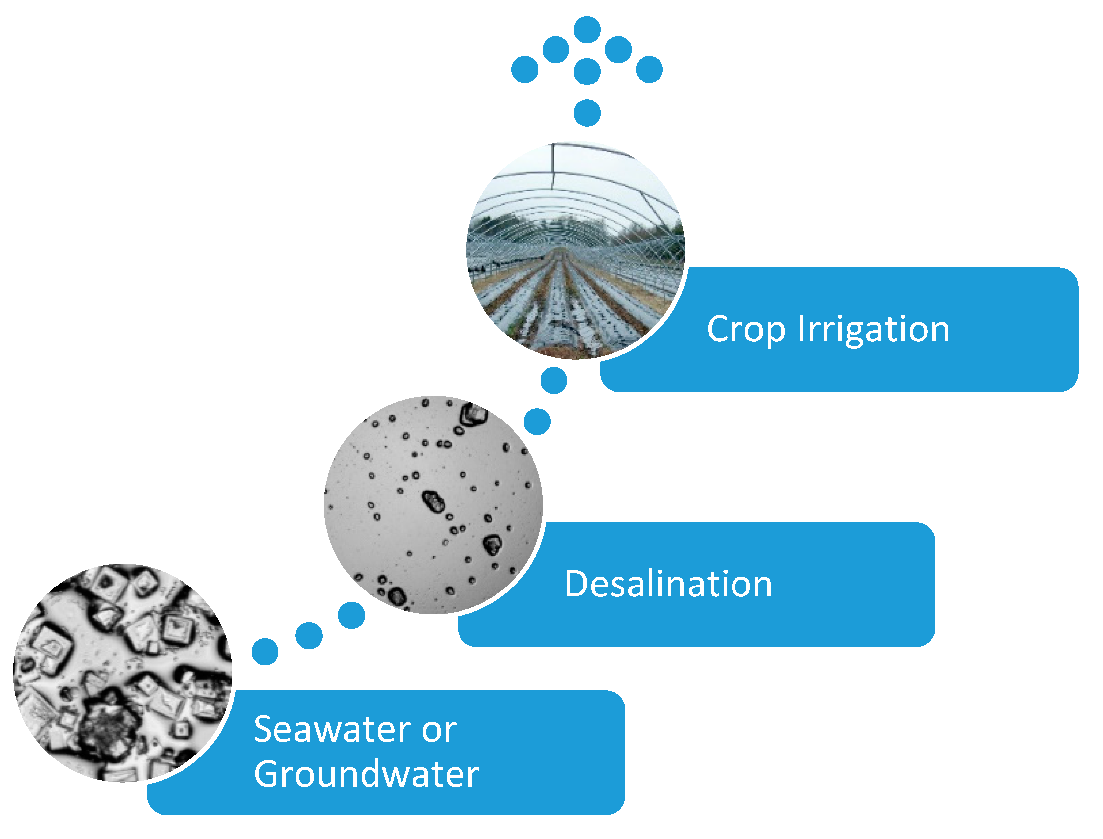
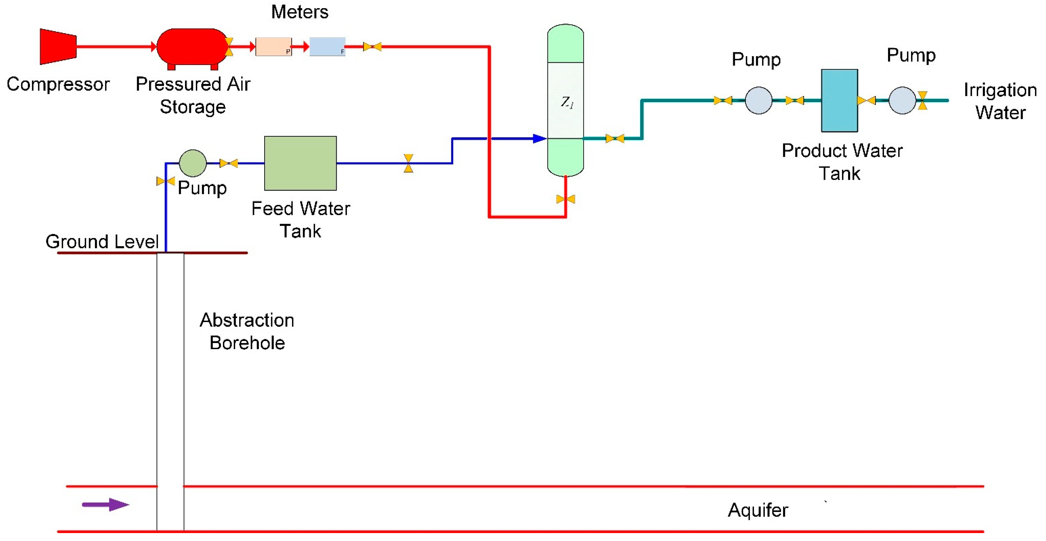
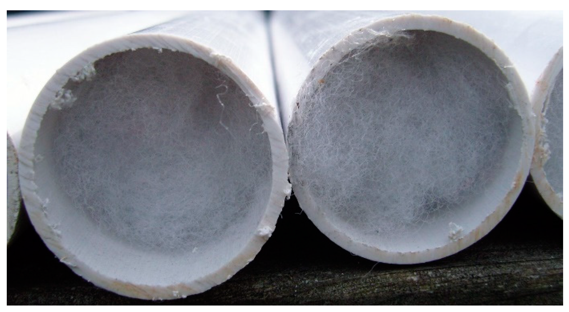
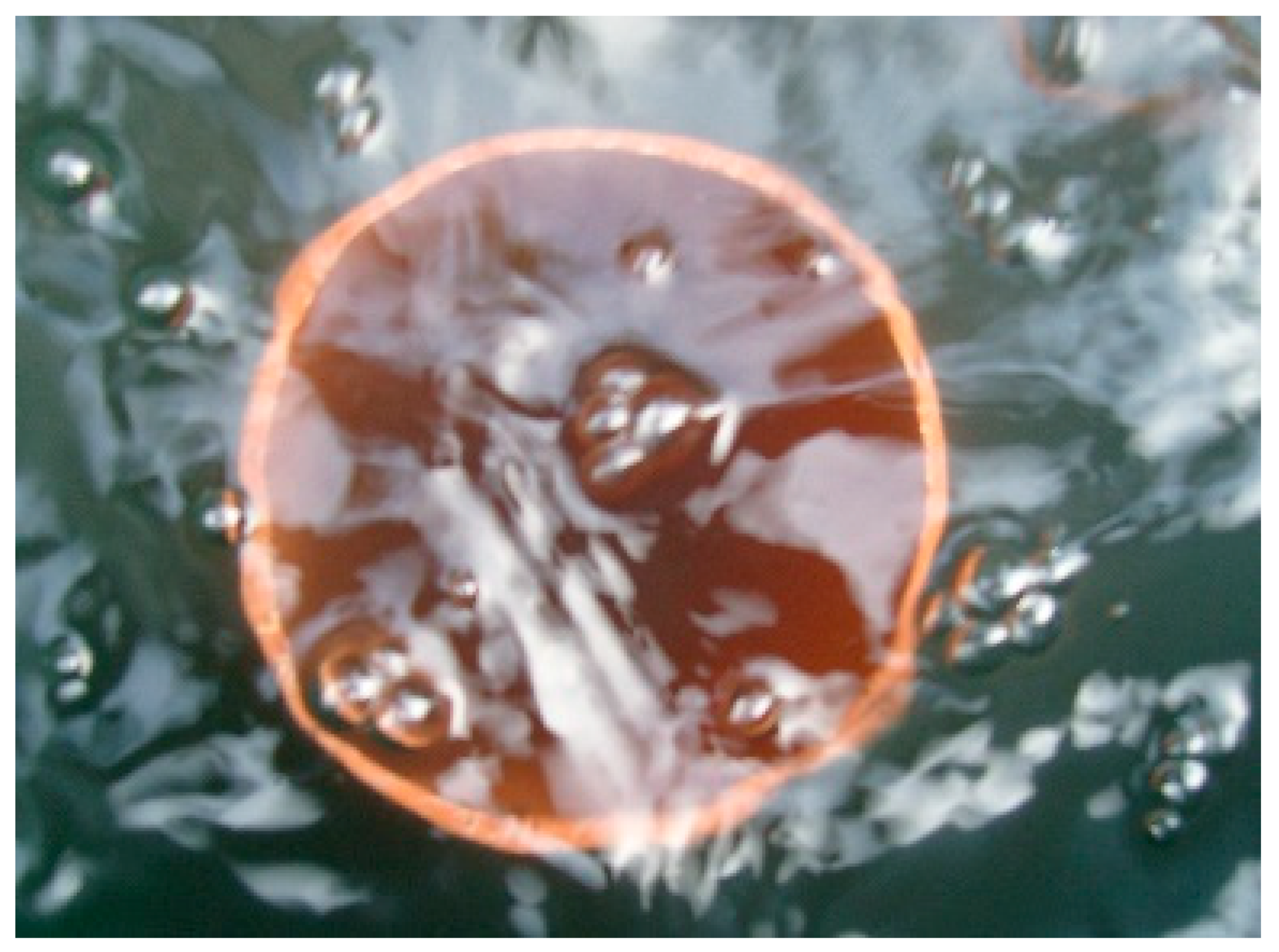
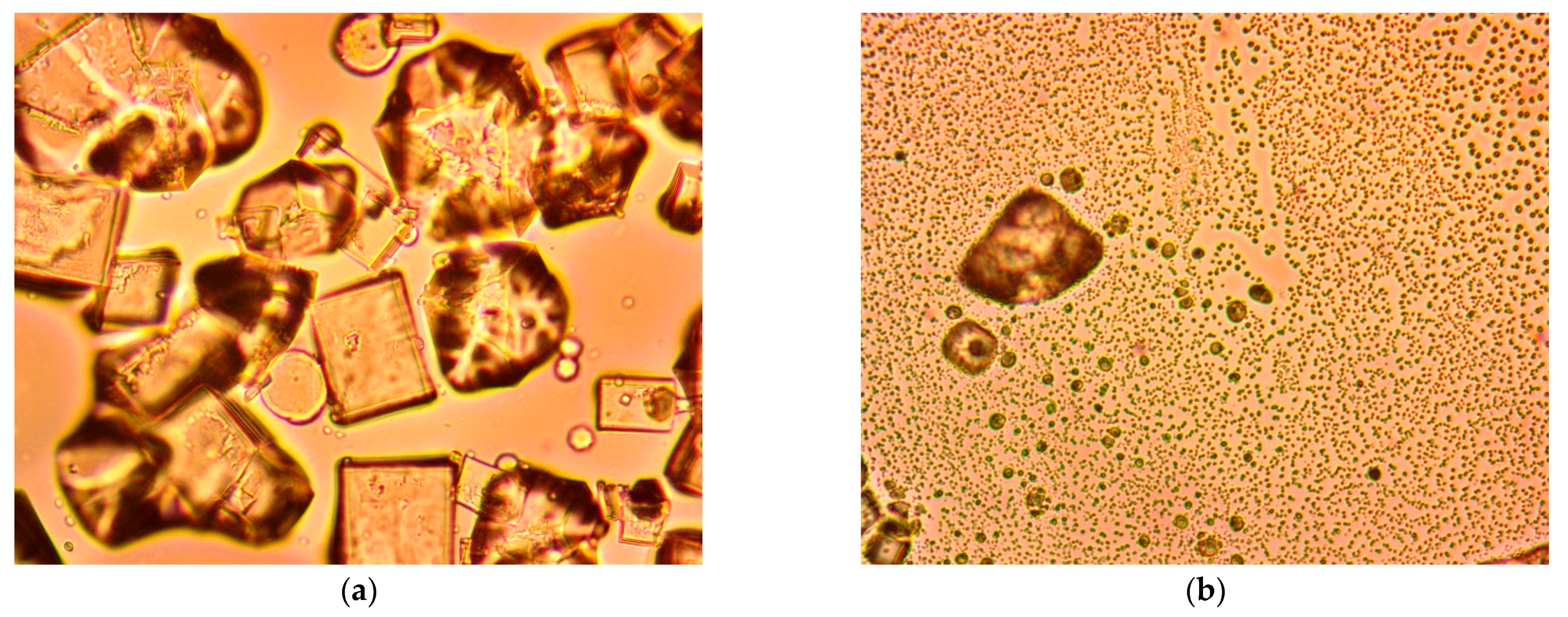
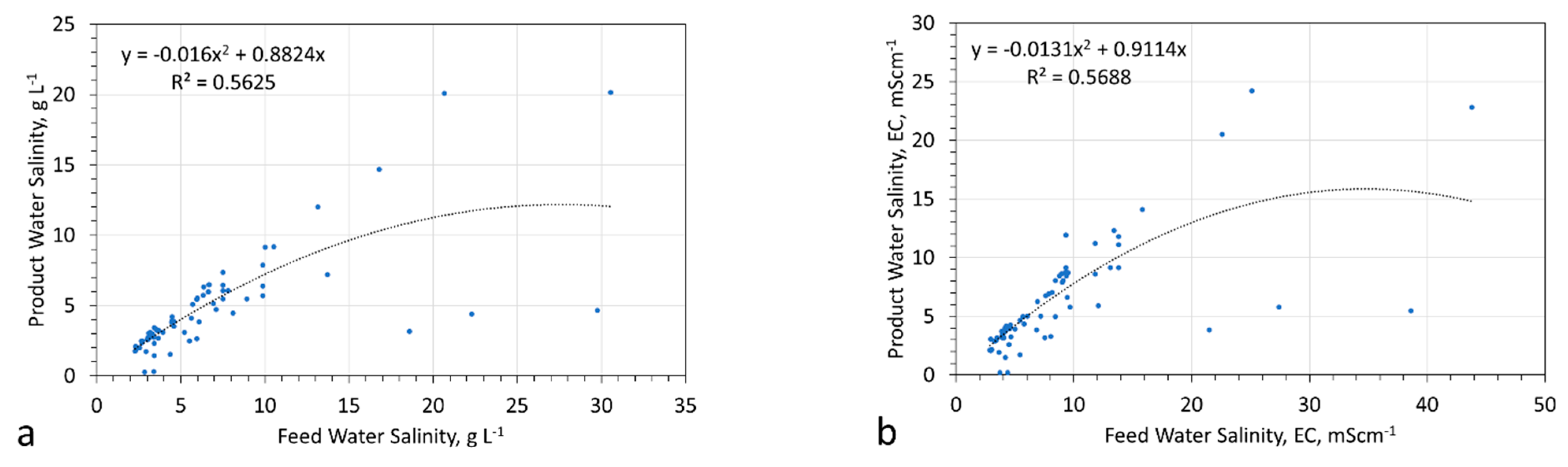
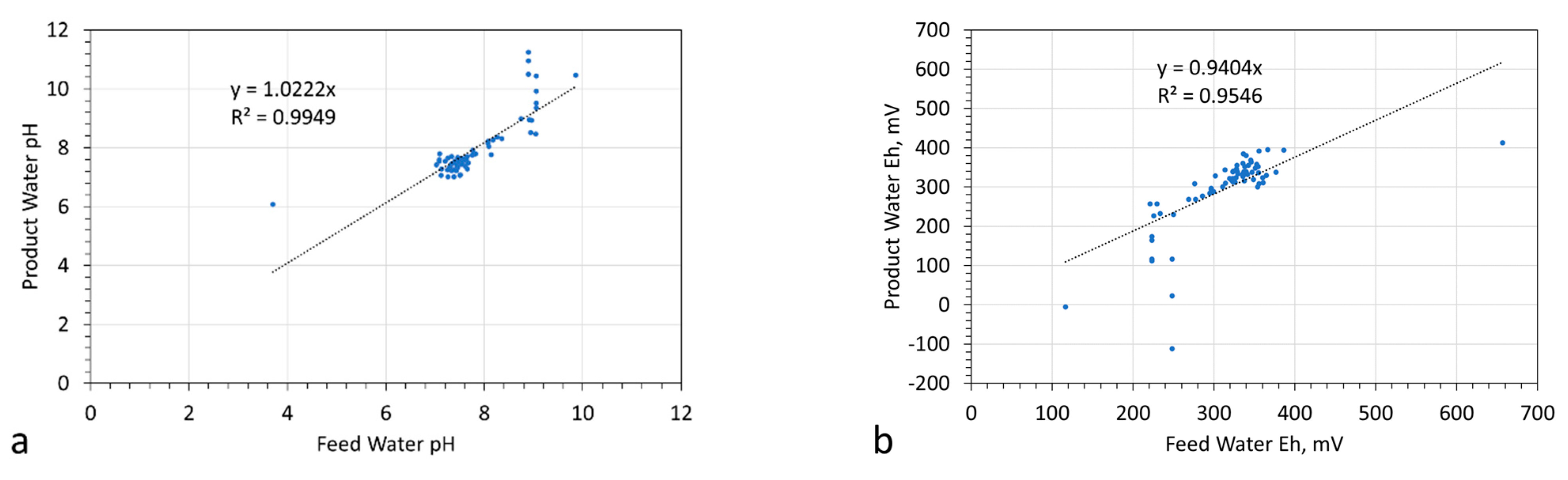
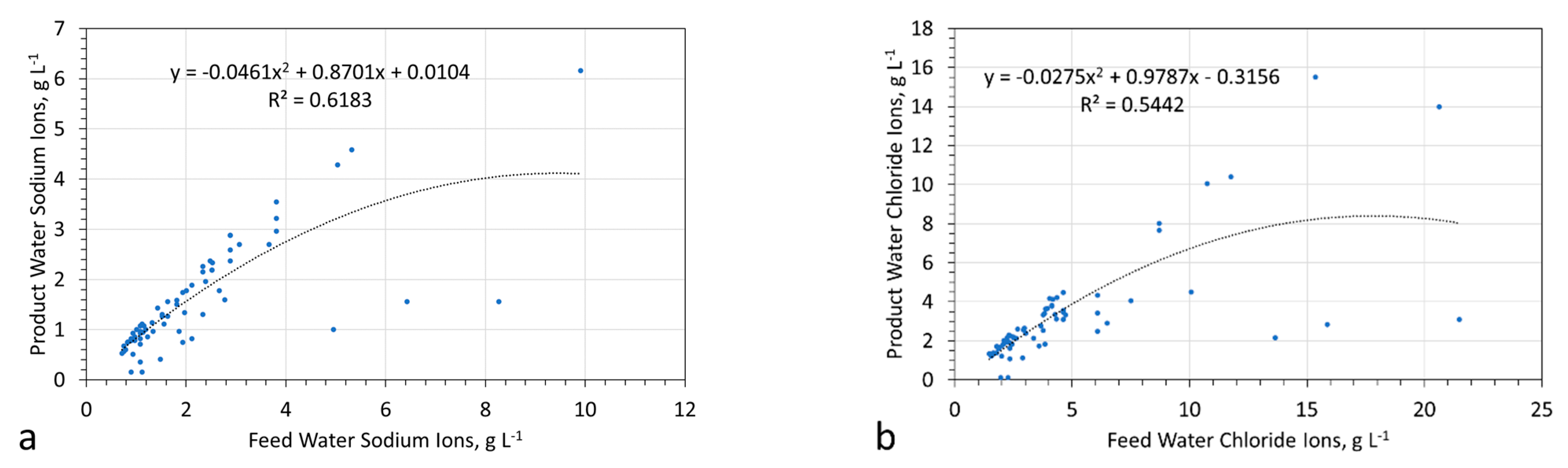
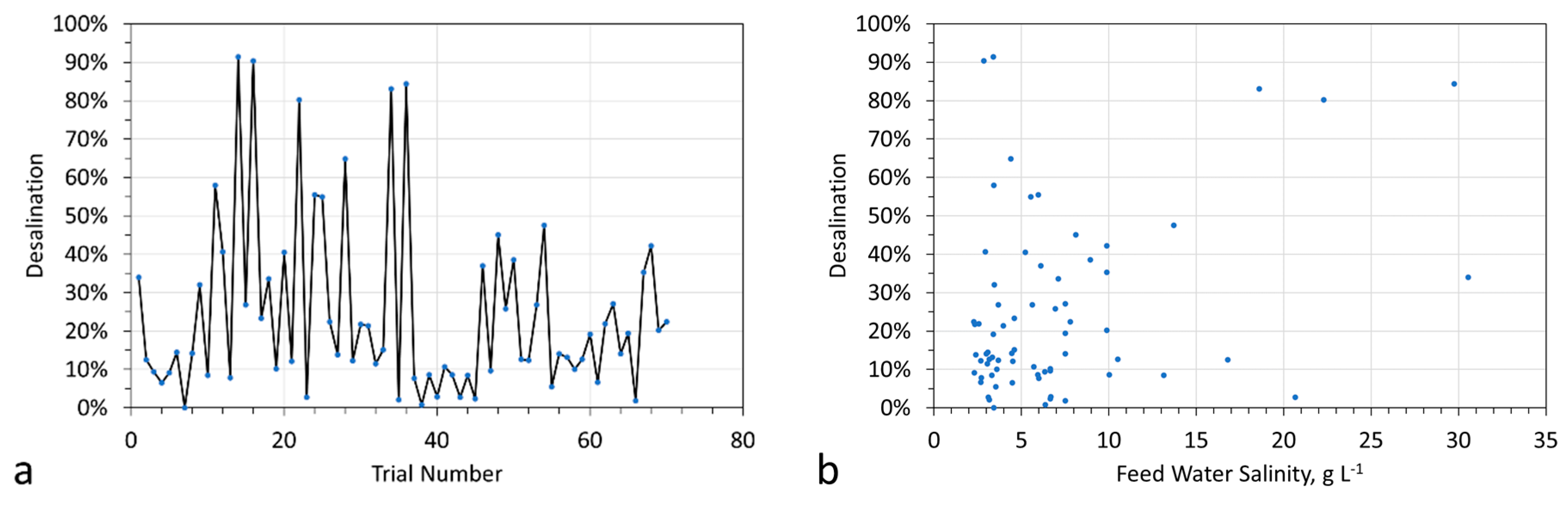
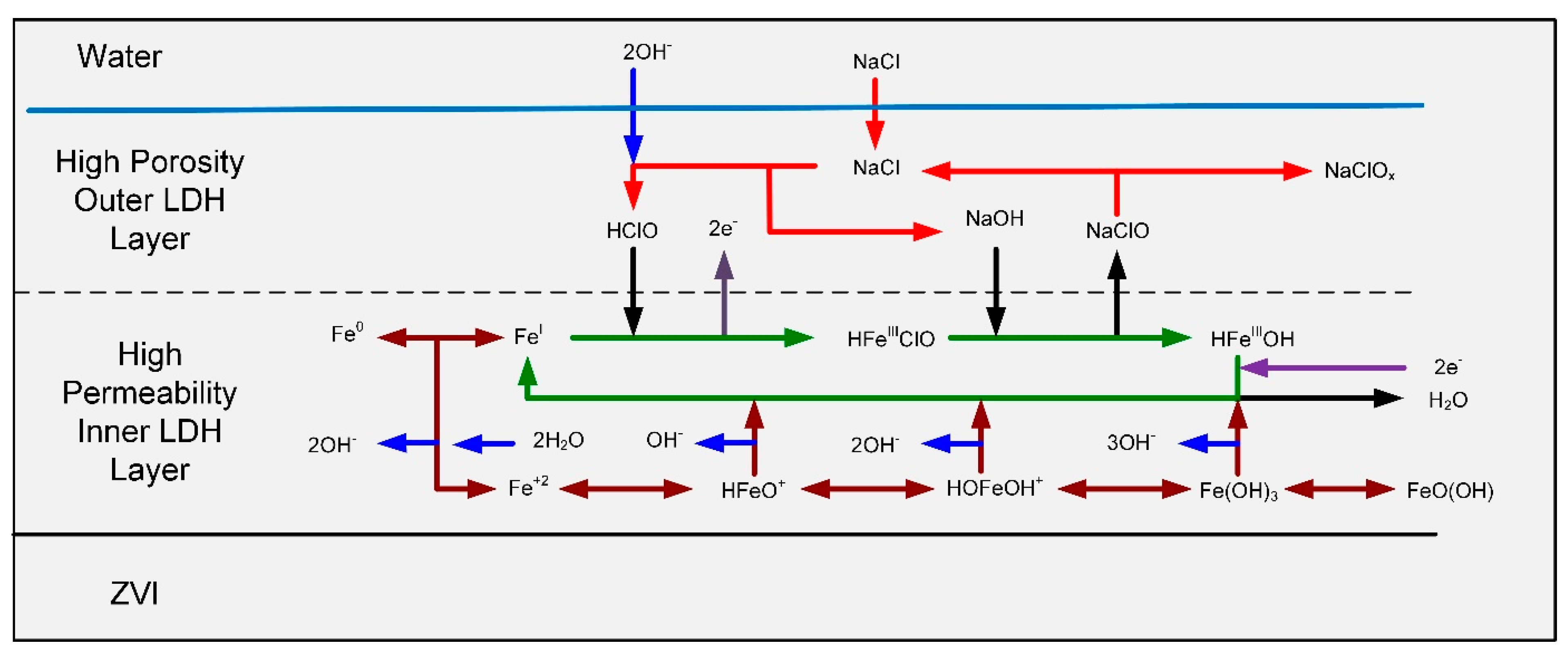
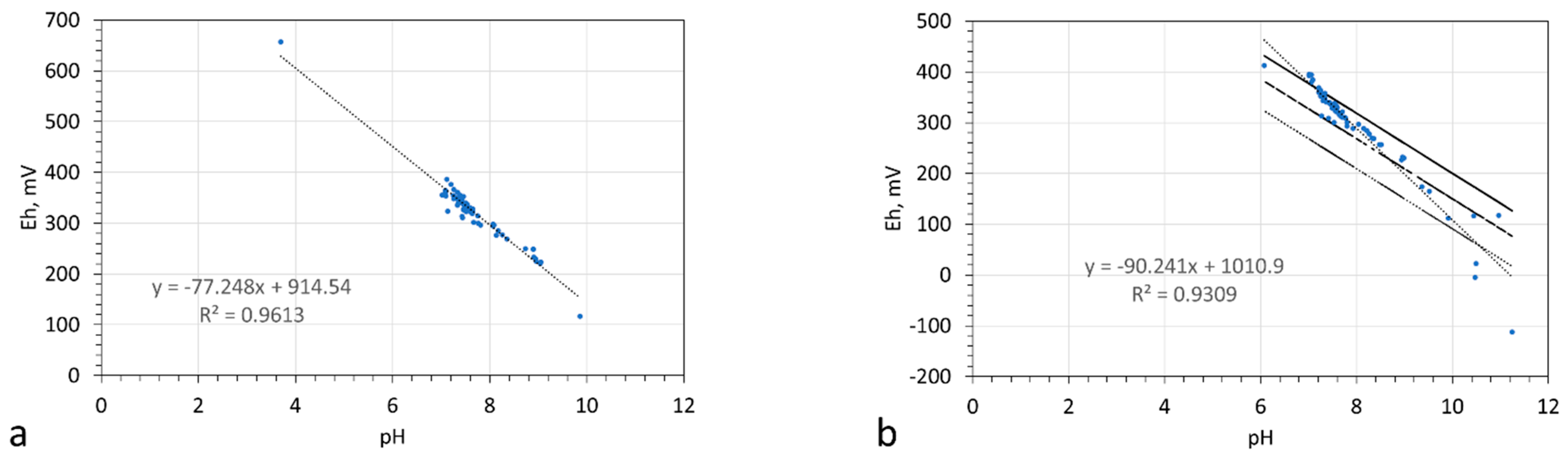
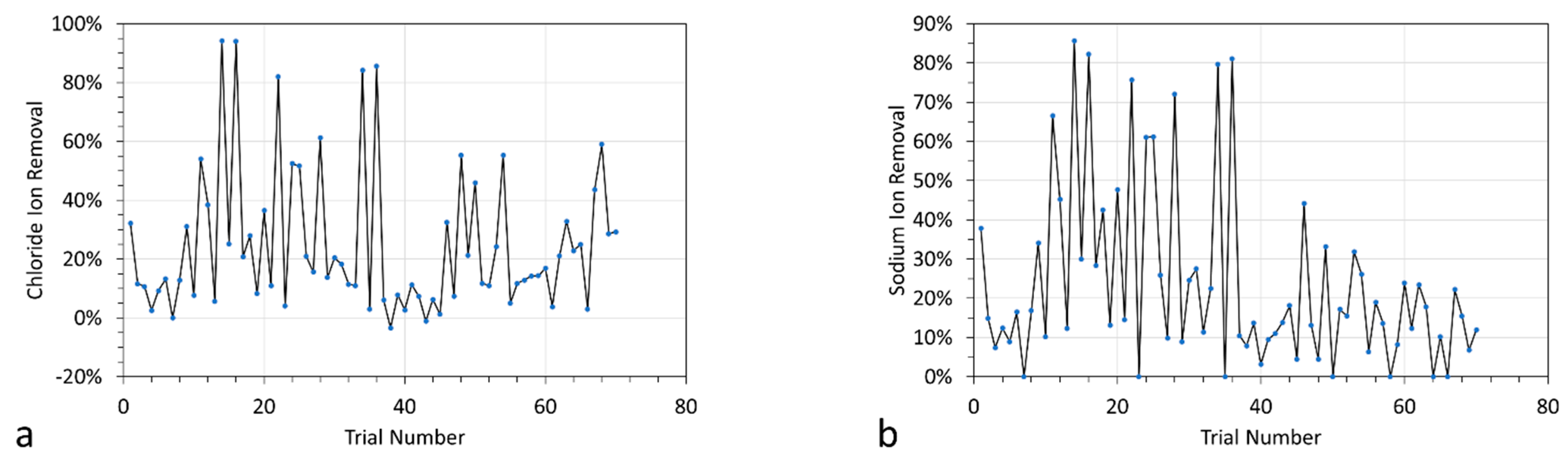
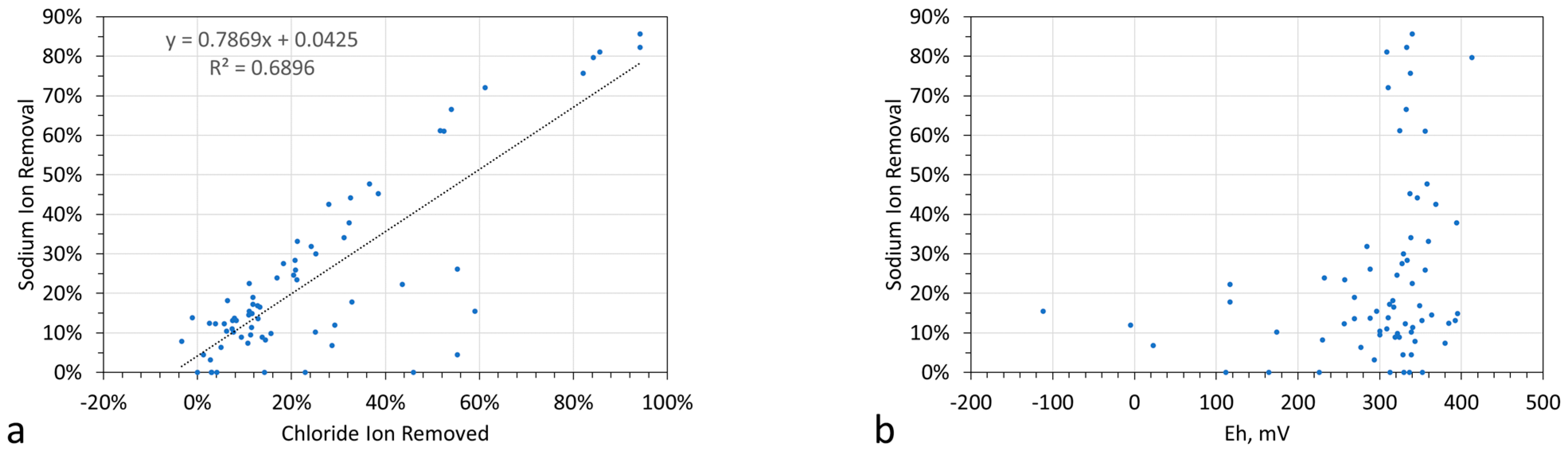
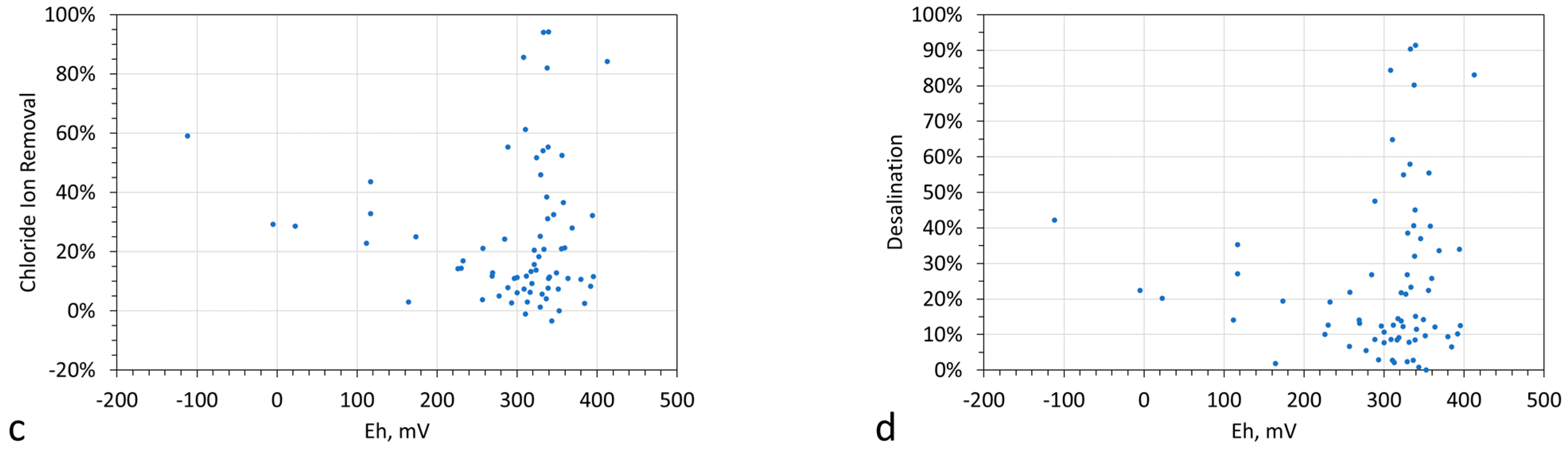
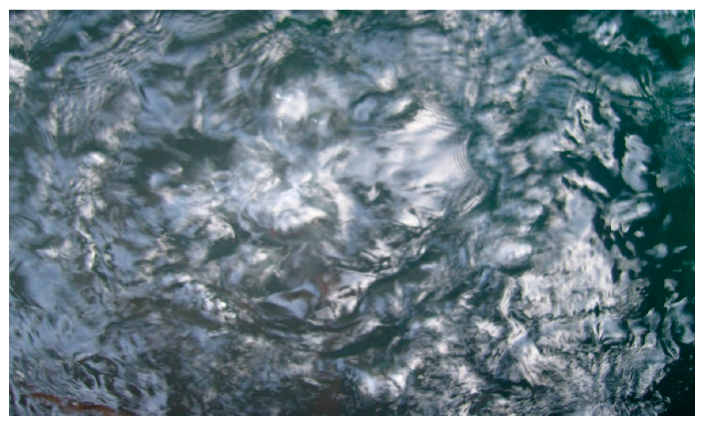
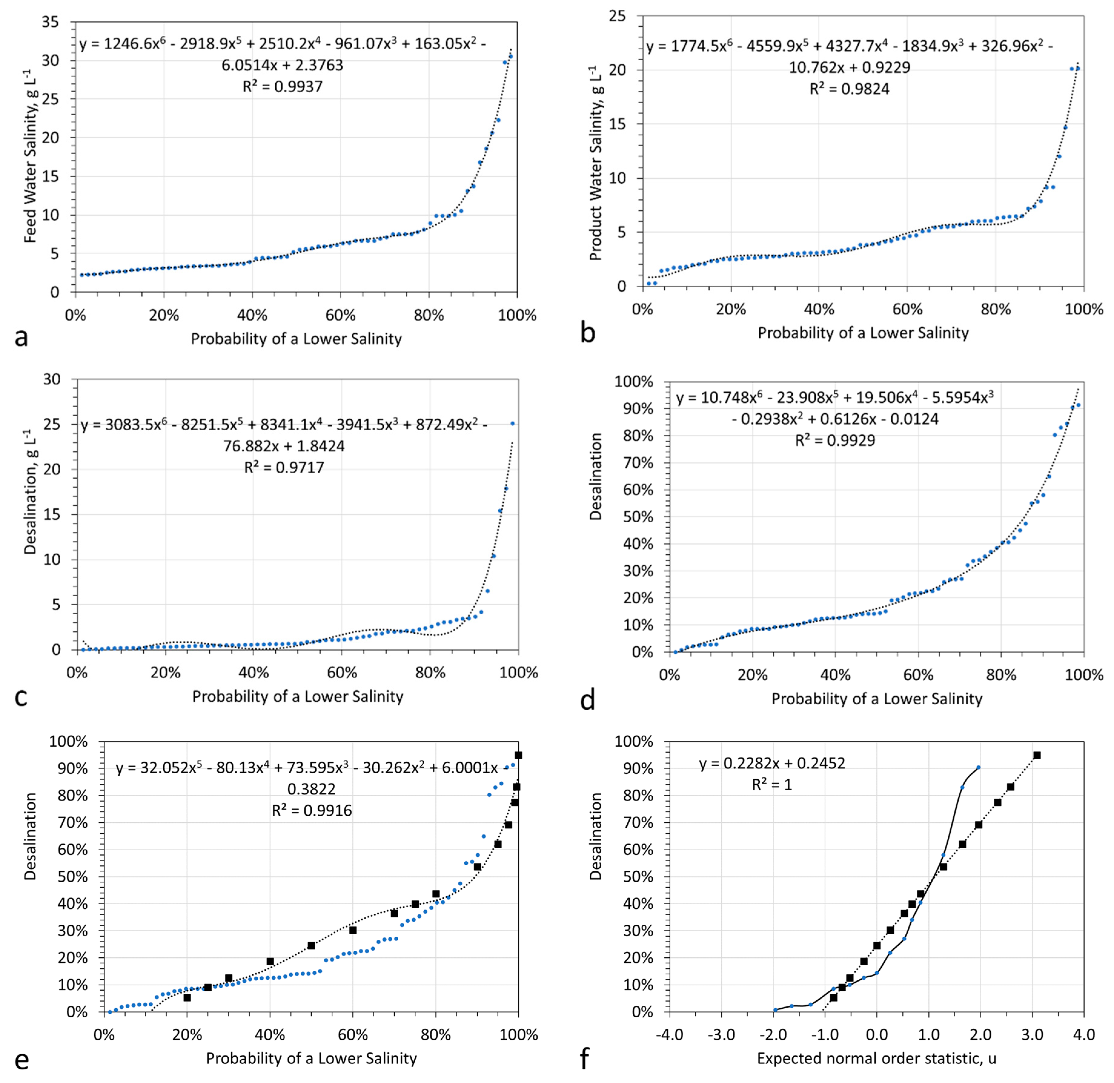
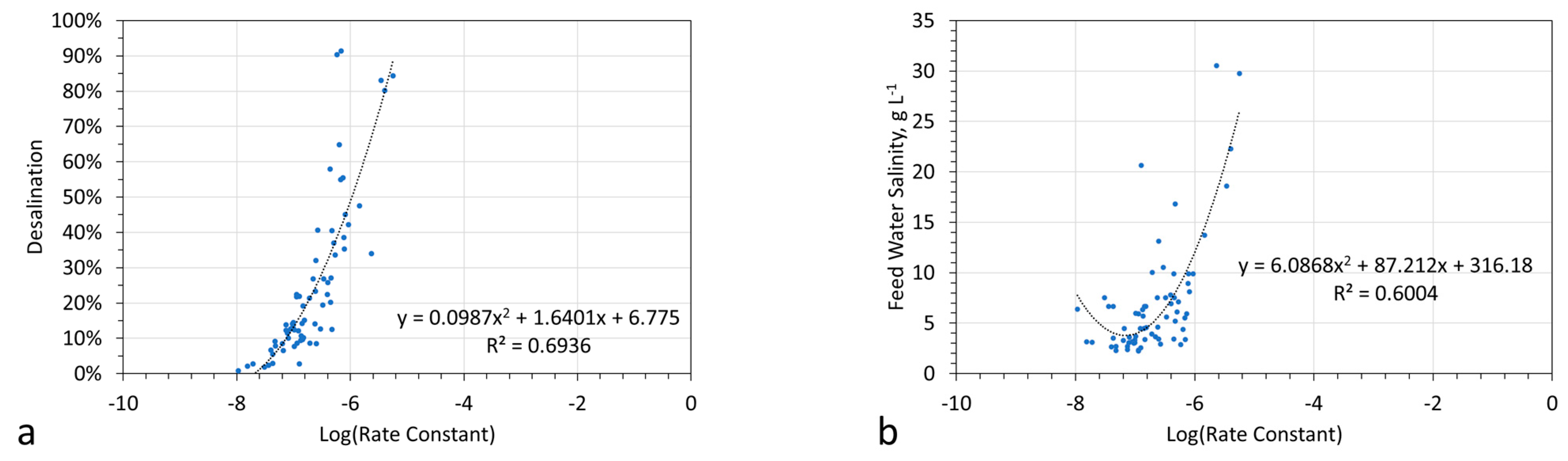
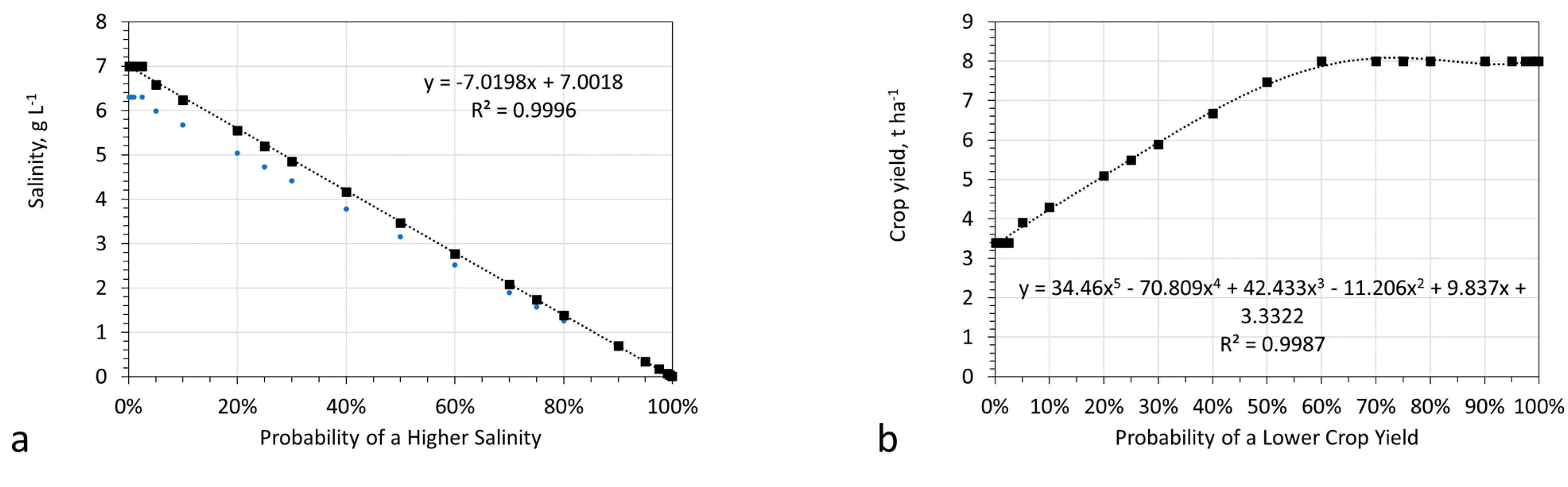
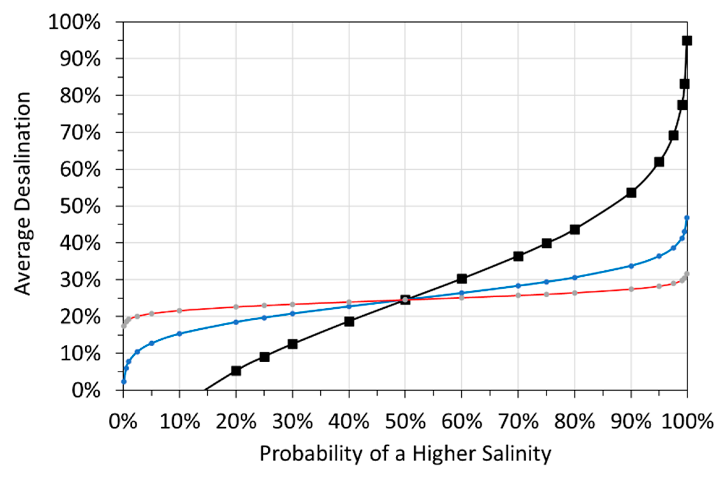
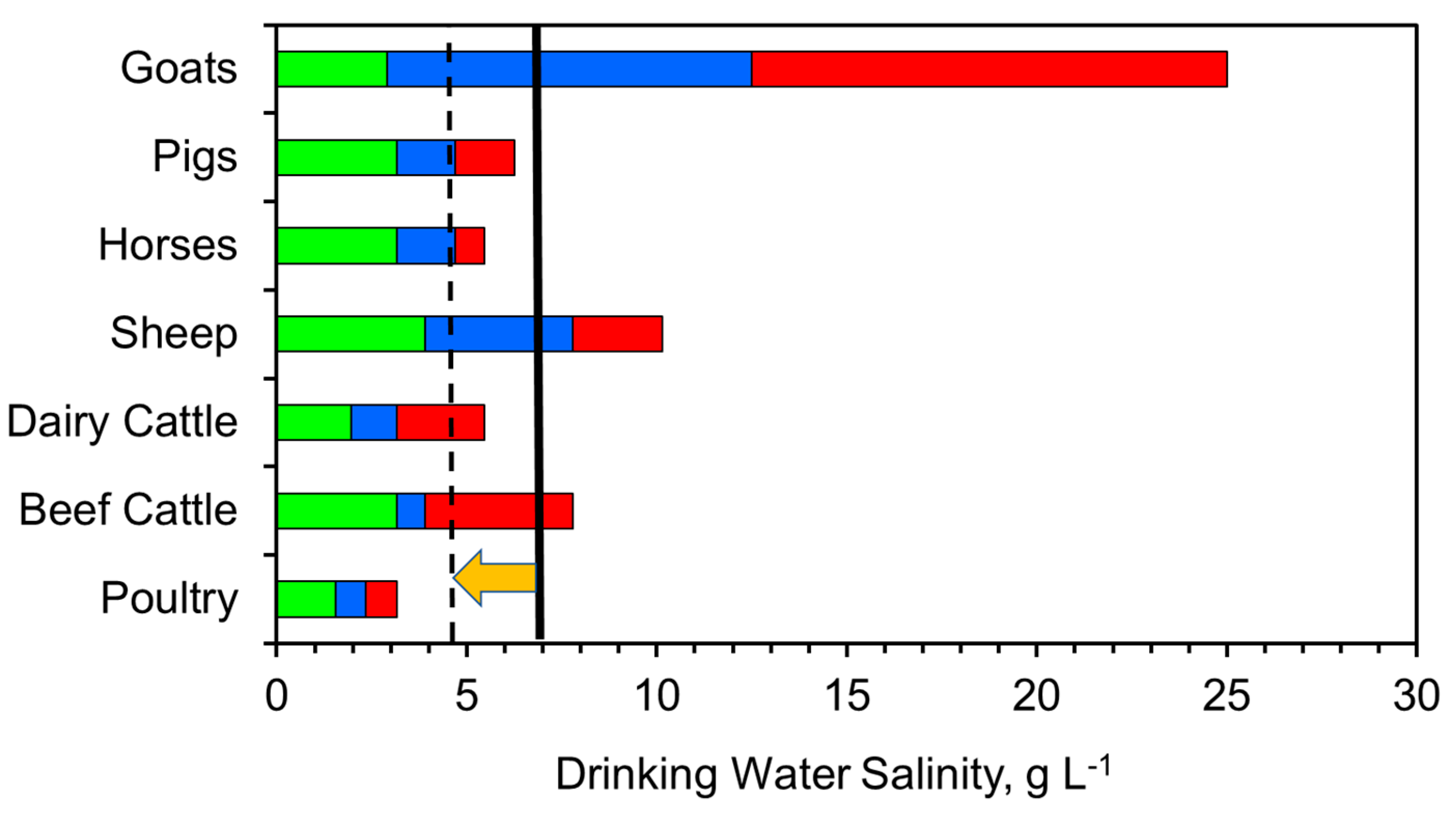
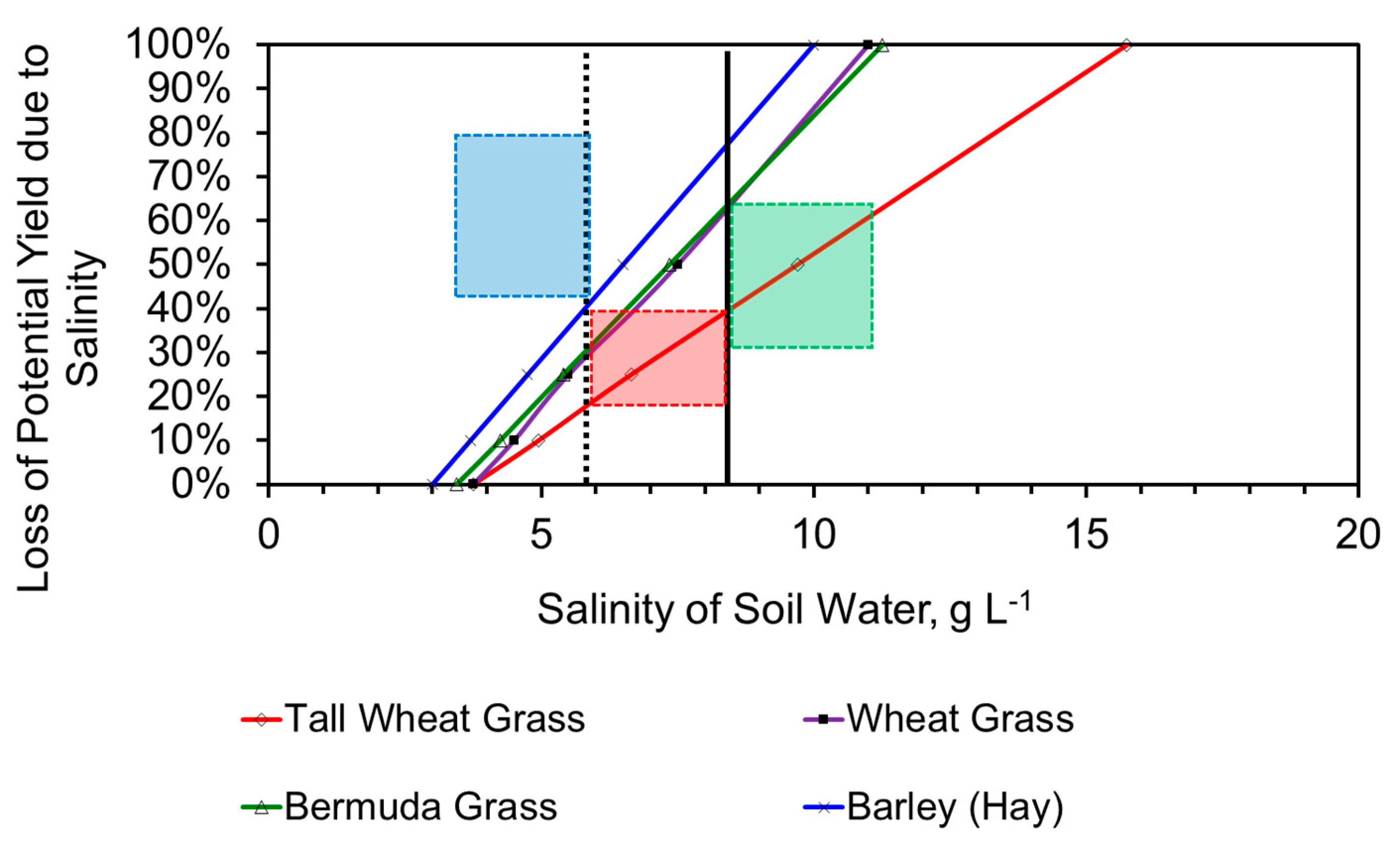
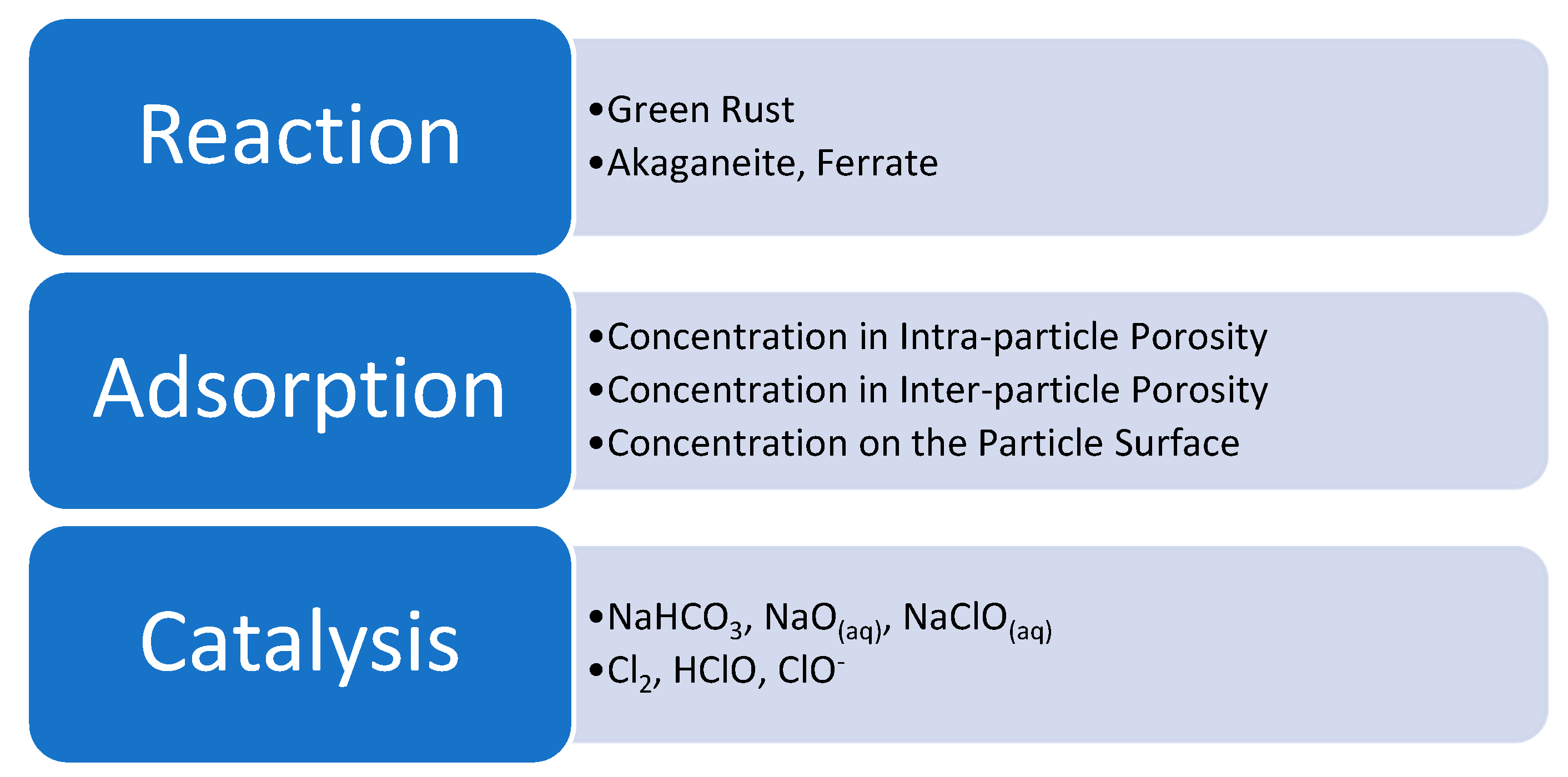
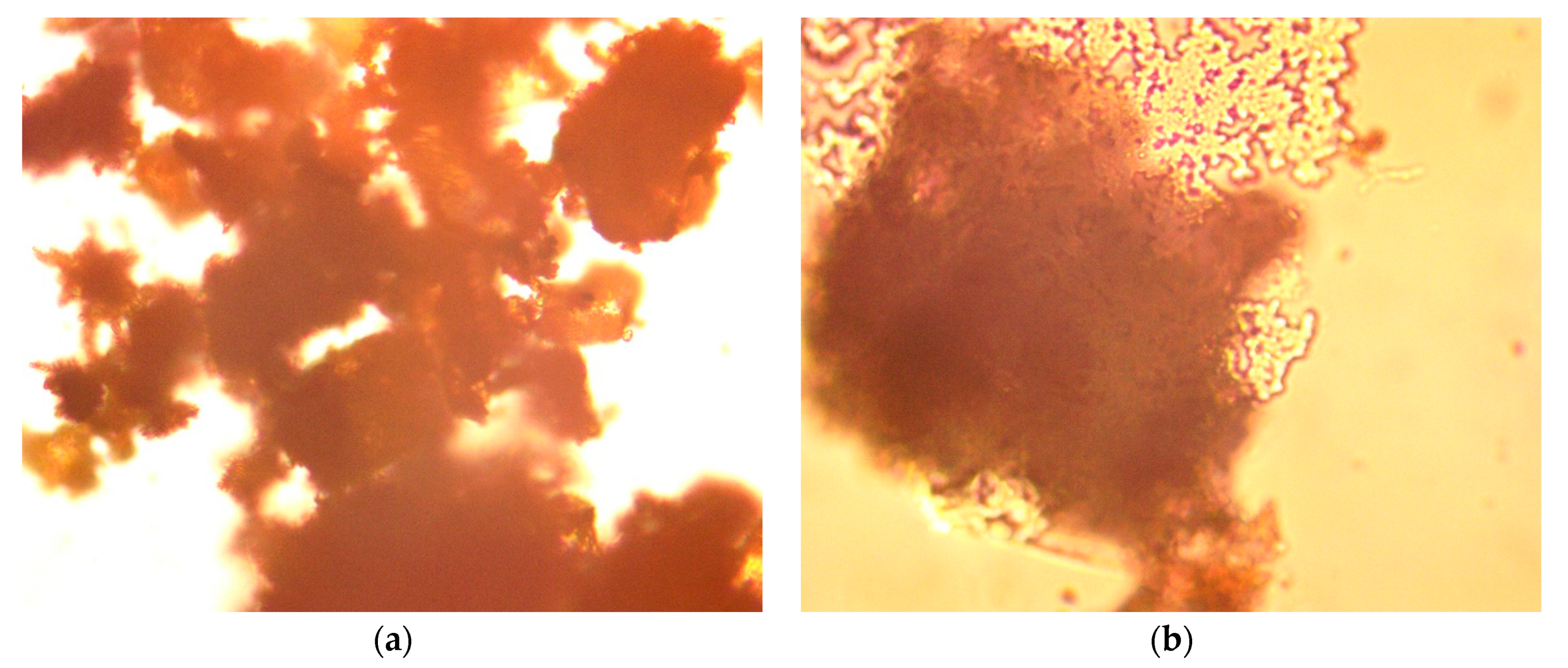
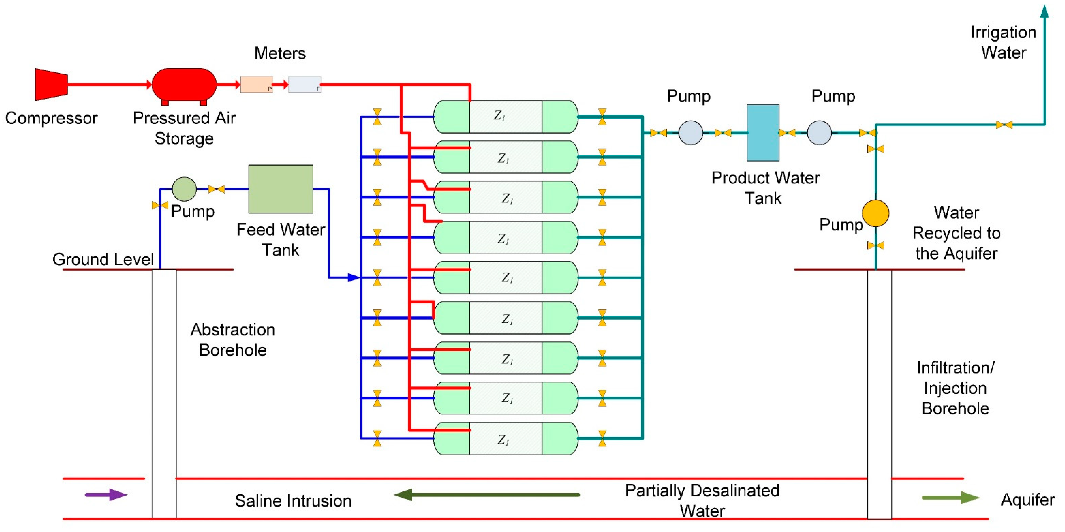
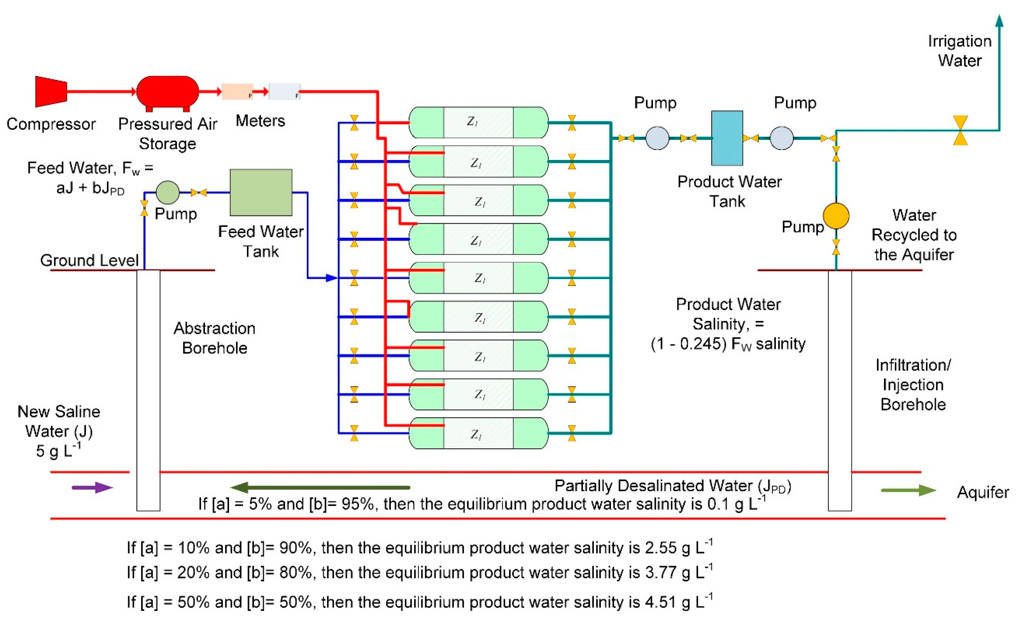
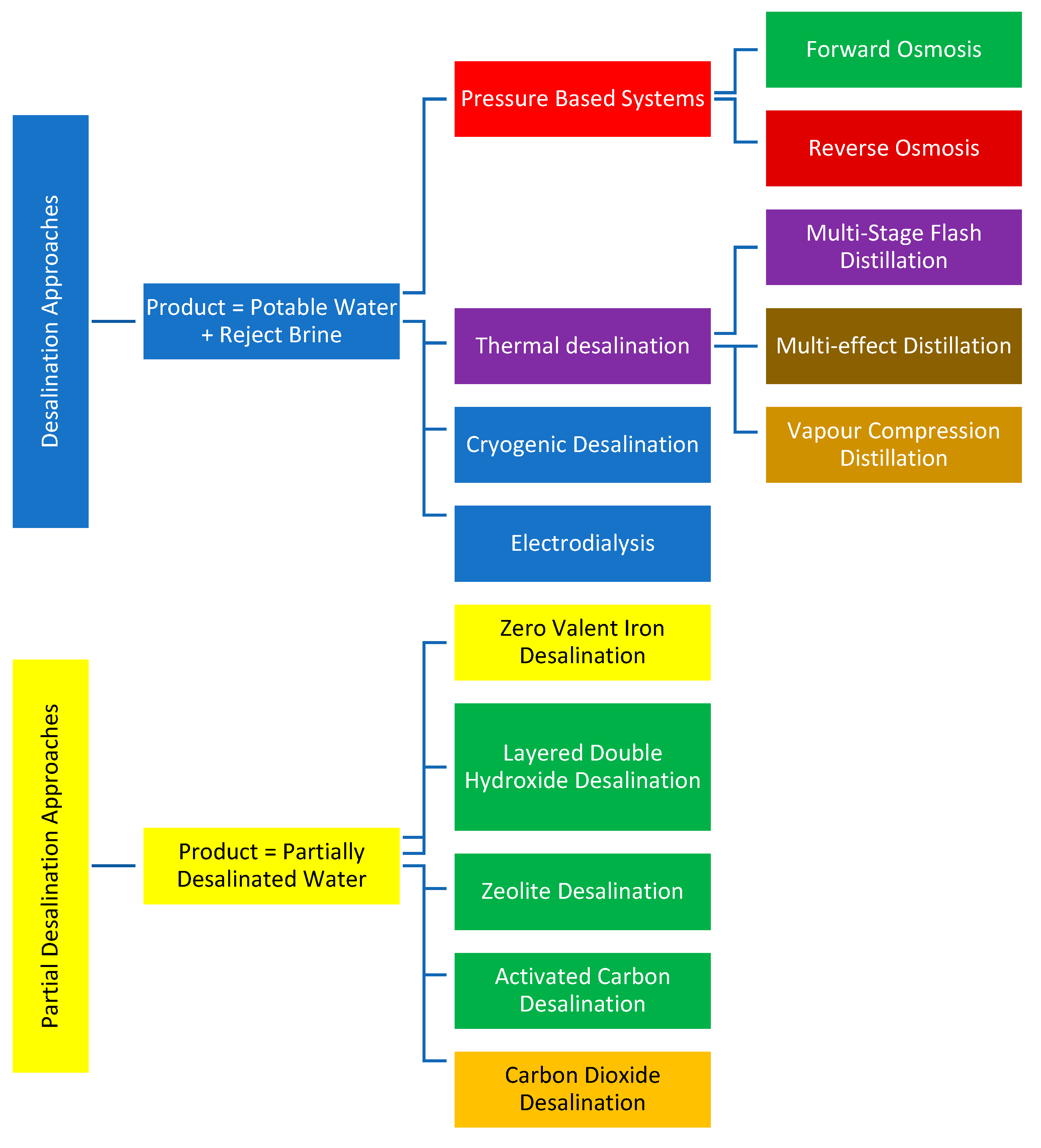
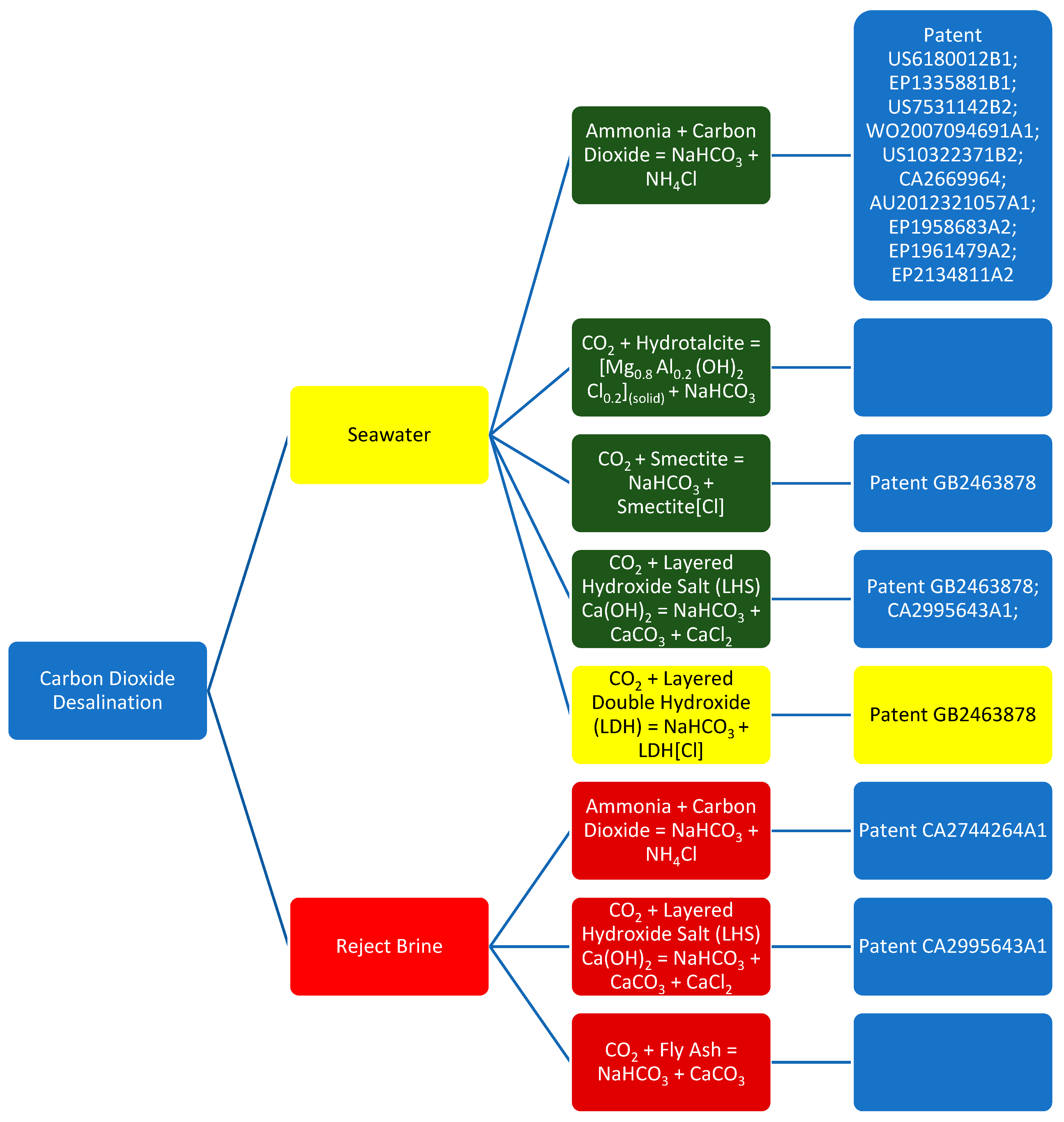
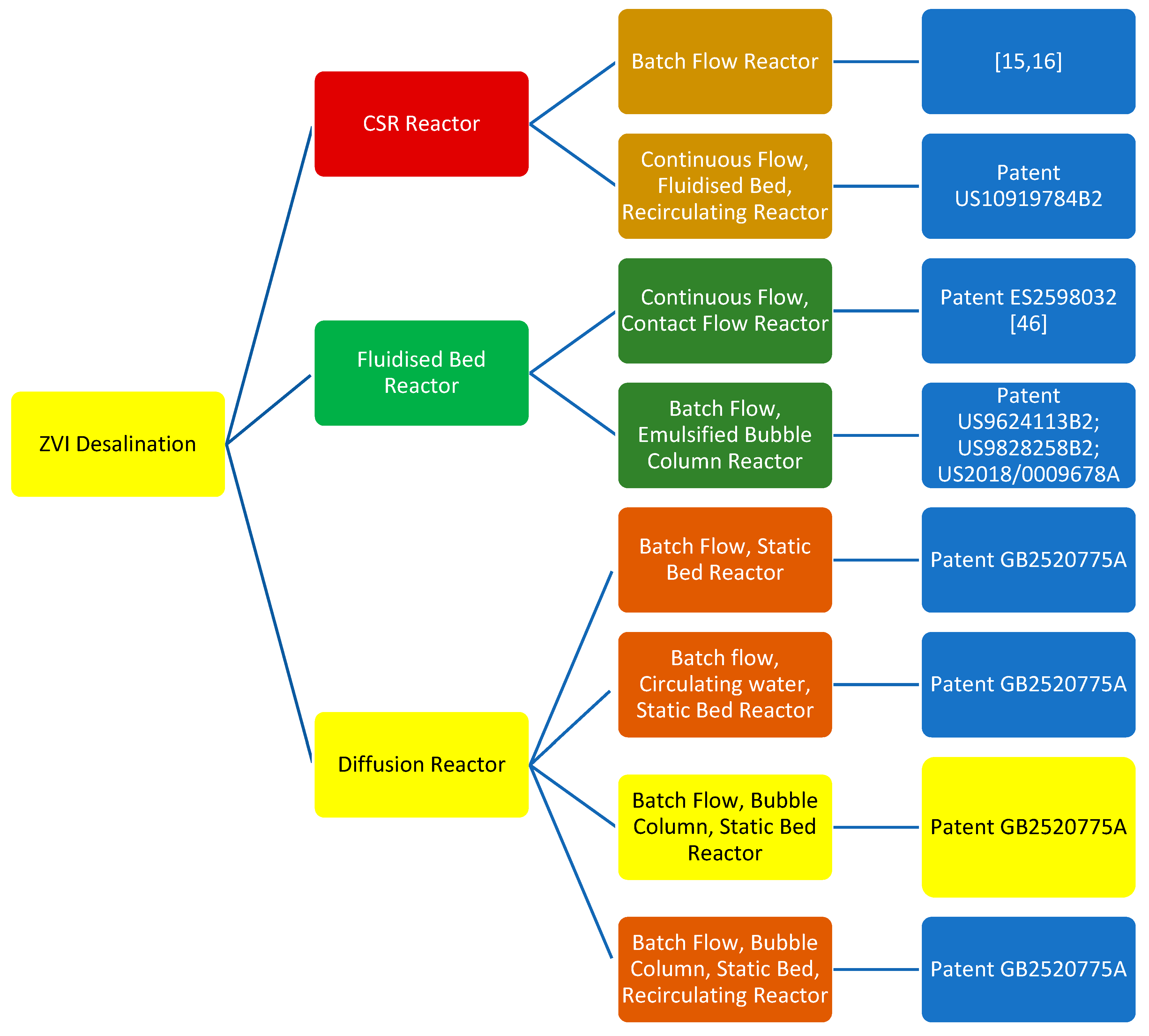
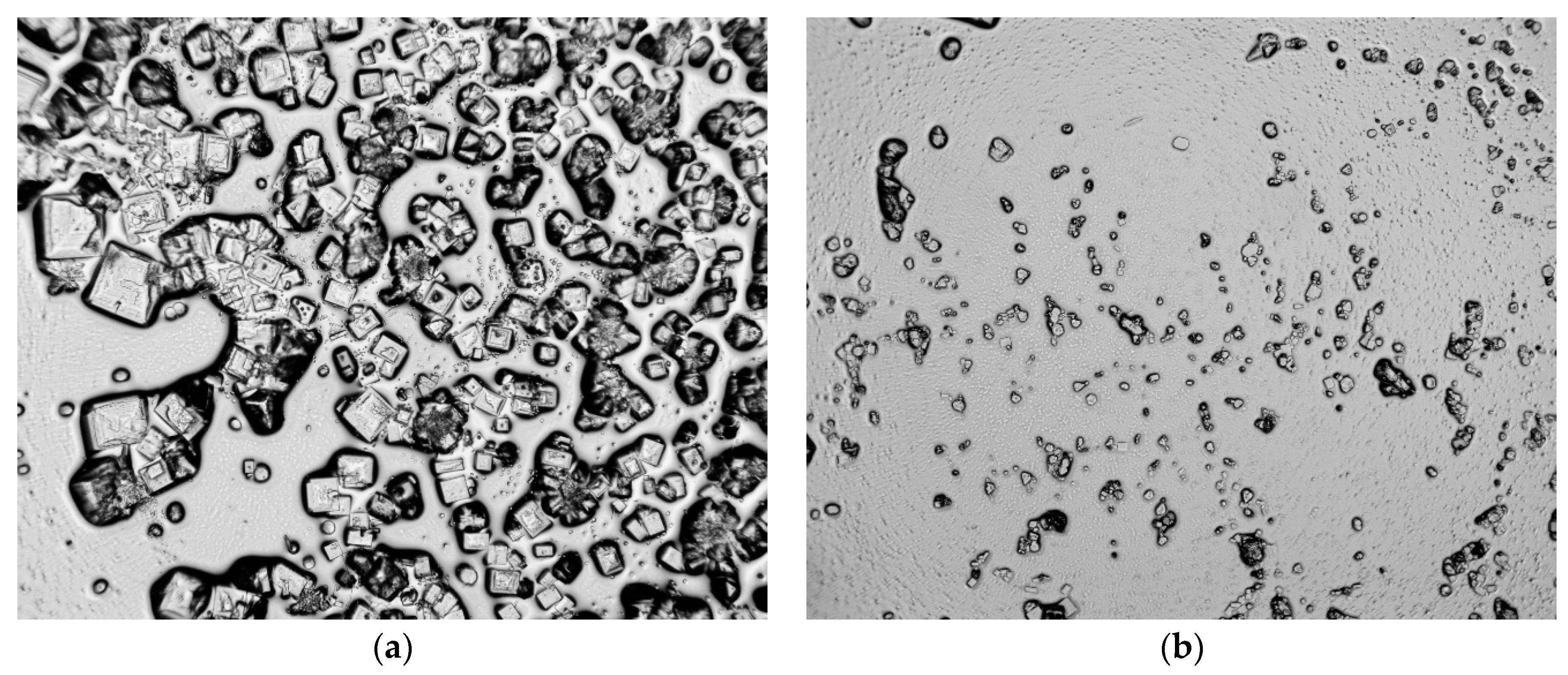
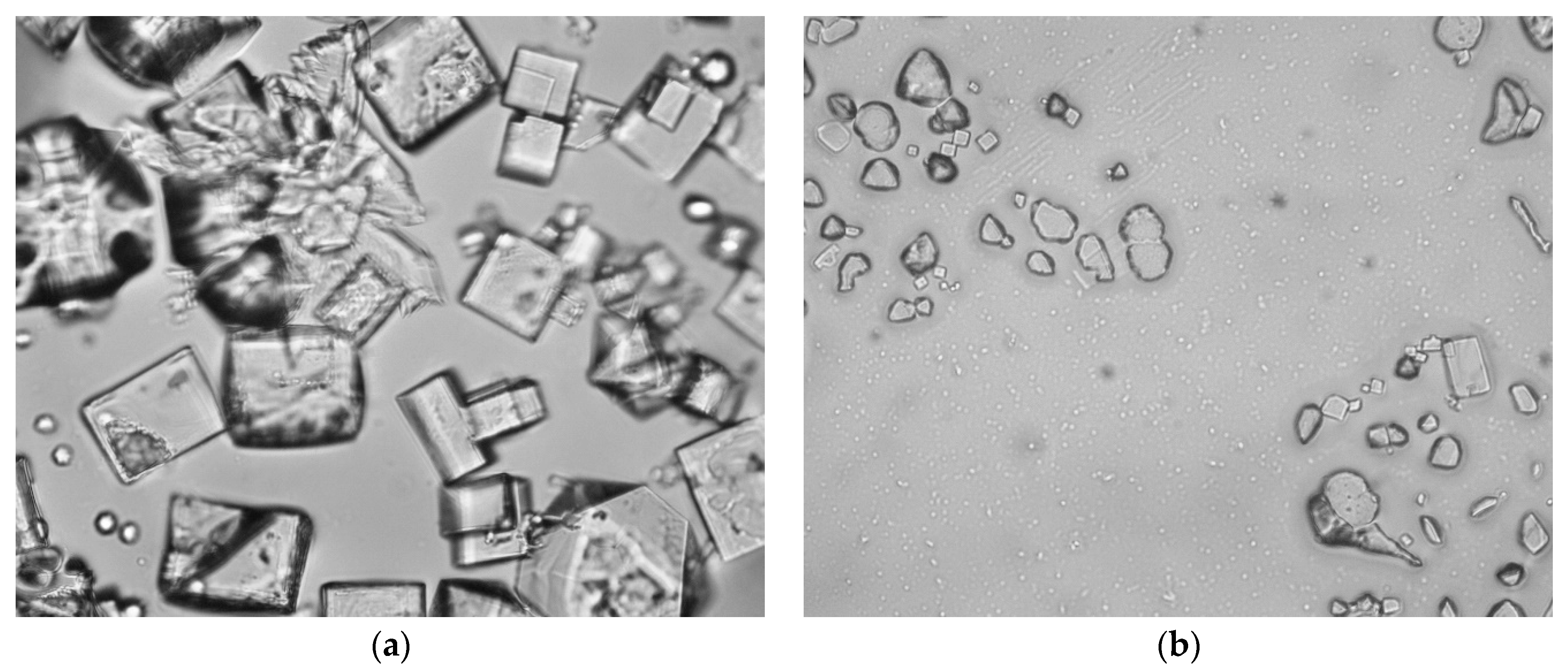
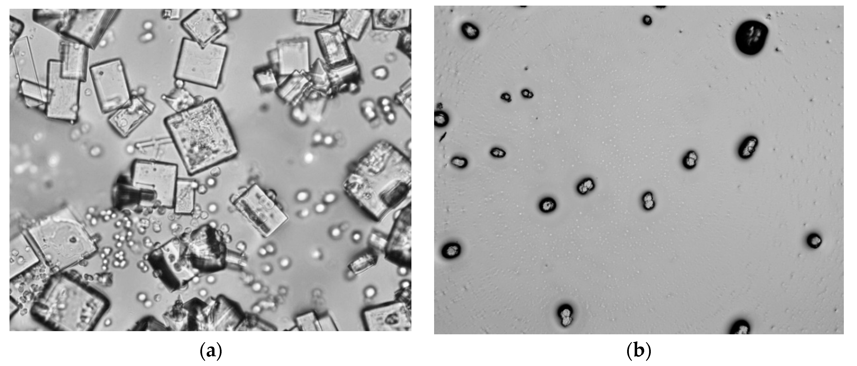
Table A1.
ZVI desalination: replication results. Fw = feed water; Pw = product water. Trials 63 to 66 and 67 to 69 are replications, where the feed water composition for each trial was identical.
Table A1.
ZVI desalination: replication results. Fw = feed water; Pw = product water. Trials 63 to 66 and 67 to 69 are replications, where the feed water composition for each trial was identical.
| Fw | Pw | |||||||||||
|---|---|---|---|---|---|---|---|---|---|---|---|---|
| Trial | pH | Eh | EC | T | Cl− | Na+ | pH | Eh | EC | T | Cl− | Na+ |
| mV | mScm−1 | C | g/L | g/L | mV | mScm−1 | C | g/L | g/L | |||
| 1 | 7.12 | 386.1 | 43.8 | 20.7 | 20.64 | 9.91 | 7.06 | 394.1 | 22.8 | 17.5 | 13.98 | 6.16 |
| 2 | 7.26 | 366.7 | 22.6 | 20.9 | 11.77 | 5.04 | 7.01 | 395.2 | 20.5 | 17.3 | 10.40 | 4.29 |
| 3 | 7.50 | 339.9 | 9.5 | 19.5 | 3.82 | 2.52 | 7.06 | 380.1 | 8.7 | 21.6 | 3.41 | 2.34 |
| 4 | 7.52 | 336.1 | 6.9 | 20.3 | 2.68 | 1.81 | 7.08 | 384.5 | 6.3 | 20.1 | 2.61 | 1.59 |
| 5 | 7.26 | 348.7 | 3.5 | 20.8 | 1.47 | 0.84 | 7.66 | 318.7 | 3.0 | 18.1 | 1.33 | 0.76 |
| 6 | 7.61 | 321.8 | 4.6 | 20.1 | 1.93 | 1.14 | 7.65 | 317.4 | 4.0 | 19.0 | 1.67 | 0.95 |
| 7 | 7.25 | 354.5 | 4.3 | 17.1 | 2.30 | 1.12 | 7.25 | 352.5 | 4.2 | 17.0 | 2.30 | 1.12 |
| 8 | 7.29 | 351.1 | 5.4 | 17.1 | 2.93 | 1.52 | 7.34 | 348.9 | 4.7 | 17.8 | 2.56 | 1.26 |
| 9 | 7.34 | 346.9 | 4.5 | 17.4 | 2.35 | 1.08 | 7.46 | 338.1 | 2.6 | 17.8 | 1.62 | 0.71 |
| 10 | 7.43 | 339.6 | 4.2 | 17.7 | 2.22 | 1.08 | 7.43 | 338.6 | 3.7 | 17.5 | 2.05 | 0.97 |
| 11 | 7.48 | 335.5 | 4.2 | 17.7 | 2.34 | 1.08 | 7.53 | 332.3 | 1.5 | 17.6 | 1.07 | 0.36 |
| 12 | 7.46 | 337.1 | 3.6 | 18.1 | 2.00 | 0.93 | 7.46 | 337.1 | 1.9 | 18.6 | 1.23 | 0.51 |
| 13 | 7.41 | 341.2 | 3.4 | 18.2 | 1.81 | 0.90 | 7.54 | 331.5 | 3.0 | 18.0 | 1.71 | 0.79 |
| 14 | 7.46 | 337.1 | 4.4 | 18.5 | 2.27 | 1.12 | 7.43 | 339.6 | 0.2 | 17.8 | 0.13 | 0.16 |
| 15 | 7.47 | 336.3 | 4.7 | 18.6 | 2.44 | 1.23 | 7.58 | 329.2 | 3.3 | 17.8 | 1.82 | 0.86 |
| 16 | 7.60 | 329.6 | 3.7 | 18.8 | 1.96 | 0.90 | 7.58 | 333.2 | 0.2 | 18.6 | 0.12 | 0.16 |
| 17 | 7.52 | 337.1 | 5.8 | 19.1 | 3.04 | 1.56 | 7.53 | 333.3 | 4.4 | 18.4 | 2.40 | 1.12 |
| 18 | 7.43 | 345.6 | 9.7 | 18.8 | 4.33 | 2.78 | 7.22 | 368.8 | 5.8 | 19.4 | 3.12 | 1.60 |
| 19 | 7.38 | 355.8 | 9.0 | 19.1 | 4.13 | 2.52 | 7.01 | 392.2 | 7.9 | 18.6 | 3.79 | 2.19 |
| 20 | 7.46 | 353.1 | 6.9 | 18.9 | 3.36 | 1.85 | 7.34 | 357.9 | 3.8 | 18.2 | 2.13 | 0.97 |
| 21 | 7.41 | 346.2 | 5.7 | 18.7 | 2.97 | 1.52 | 7.25 | 363.5 | 5.0 | 18.7 | 2.64 | 1.30 |
| 22 | 7.20 | 376.6 | 27.4 | 19.5 | 15.86 | 6.42 | 7.54 | 337.5 | 5.8 | 20.1 | 2.85 | 1.56 |
| 23 | 7.40 | 355.0 | 4.1 | 20.6 | 2.10 | 1.01 | 7.54 | 336.5 | 4.0 | 20.1 | 2.01 | 1.01 |
| 24 | 7.65 | 328.4 | 8.1 | 18.7 | 3.84 | 2.11 | 7.28 | 355.9 | 3.3 | 19.5 | 1.82 | 0.82 |
| 25 | 7.64 | 327.2 | 7.5 | 20.1 | 3.60 | 1.93 | 7.59 | 324.4 | 3.2 | 19.4 | 1.74 | 0.75 |
| 26 | 7.42 | 342.4 | 2.9 | 19.8 | 1.55 | 0.71 | 7.26 | 355.7 | 2.1 | 20.8 | 1.23 | 0.53 |
| 27 | 7.65 | 323.4 | 2.9 | 21.0 | 1.64 | 0.75 | 7.71 | 321.5 | 3.1 | 19.3 | 1.38 | 0.67 |
| 28 | 7.76 | 314.4 | 5.5 | 19.2 | 2.90 | 1.49 | 7.76 | 310.4 | 1.7 | 19.2 | 1.13 | 0.41 |
| 29 | 7.08 | 360.5 | 3.3 | 19.4 | 1.86 | 0.82 | 7.55 | 323.8 | 2.9 | 20.2 | 1.60 | 0.75 |
| 30 | 7.64 | 319.2 | 2.9 | 20.6 | 1.59 | 0.75 | 7.58 | 321.2 | 2.1 | 20.2 | 1.26 | 0.56 |
| 31 | 7.49 | 335.7 | 5.0 | 20.0 | 2.61 | 1.34 | 7.58 | 327.2 | 3.9 | 18.6 | 2.13 | 0.97 |
| 32 | 7.61 | 323.8 | 3.9 | 19.5 | 2.08 | 0.97 | 7.37 | 340.6 | 3.4 | 19.4 | 1.84 | 0.86 |
| 33 | 7.55 | 328.8 | 6.1 | 19.7 | 2.95 | 1.63 | 7.43 | 339.6 | 5.0 | 19.9 | 2.63 | 1.26 |
| 34 | 3.70 | 656.7 | 21.5 | 18.2 | 13.64 | 4.95 | 6.08 | 412.7 | 3.8 | 18.5 | 2.15 | 1.01 |
| 35 | 7.13 | 323.3 | 3.9 | 19.1 | 2.23 | 0.93 | 7.28 | 312.9 | 3.7 | 18.5 | 2.17 | 0.93 |
| 36 | 7.02 | 355.4 | 38.6 | 19.5 | 21.49 | 8.27 | 7.42 | 308.4 | 5.5 | 18.8 | 3.09 | 1.56 |
| 37 | 7.44 | 310.8 | 7.9 | 19.1 | 3.87 | 2.11 | 7.53 | 300.3 | 6.9 | 18.6 | 3.63 | 1.89 |
| 38 | 7.43 | 313.6 | 8.4 | 19.4 | 4.04 | 2.33 | 7.30 | 343.3 | 8.1 | 19.6 | 4.18 | 2.15 |
| 39 | 7.77 | 299.6 | 11.8 | 20.6 | 8.70 | 1.32 | 7.92 | 288.3 | 11.2 | 20.5 | 8.02 | 1.14 |
| 40 | 7.82 | 296.4 | 8.8 | 21.5 | 4.35 | 2.33 | 7.80 | 293.2 | 8.5 | 19.9 | 4.23 | 2.26 |
| 41 | 7.10 | 353.7 | 7.6 | 22.1 | 3.77 | 1.93 | 7.80 | 300.2 | 6.8 | 20.2 | 3.34 | 1.74 |
| 42 | 8.14 | 276.1 | 8.2 | 19.7 | 3.94 | 2.00 | 7.77 | 308.6 | 7.0 | 19.6 | 3.65 | 1.78 |
| 43 | 7.34 | 360.9 | 25.1 | 20.7 | 15.35 | 5.32 | 7.71 | 310.5 | 24.2 | 17.0 | 15.52 | 4.58 |
| 44 | 7.54 | 337.5 | 15.8 | 20.0 | 10.74 | 2.39 | 7.64 | 316.2 | 14.1 | 16.9 | 10.06 | 1.96 |
| 45 | 7.67 | 301.9 | 9.0 | 22.3 | 4.18 | 2.48 | 7.49 | 328.7 | 8.6 | 21.2 | 4.13 | 2.37 |
| 46 | 7.46 | 328.1 | 8.4 | 23.0 | 3.77 | 2.33 | 7.34 | 345.9 | 5.0 | 21.6 | 2.54 | 1.30 |
| 47 | 7.35 | 338.1 | 9.1 | 21.6 | 4.13 | 2.52 | 7.26 | 351.7 | 8.1 | 21.0 | 3.82 | 2.19 |
| 48 | 7.52 | 323.1 | 12.1 | 21.7 | 6.48 | 1.63 | 7.43 | 338.6 | 5.9 | 20.7 | 2.90 | 1.56 |
| 49 | 7.34 | 335.9 | 9.5 | 21.3 | 4.26 | 2.66 | 7.22 | 359.8 | 6.6 | 20.2 | 3.36 | 1.78 |
| 50 | 7.08 | 364.5 | 11.8 | 21.7 | 7.50 | 1.43 | 7.60 | 329.6 | 8.6 | 19.8 | 4.06 | 1.43 |
| 51 | 7.46 | 326.1 | 13.4 | 20.7 | 8.70 | 1.82 | 7.67 | 311.9 | 12.3 | 20.8 | 7.67 | 1.50 |
| 52 | 8.09 | 296.3 | 4.6 | 17.9 | 2.49 | 1.19 | 8.04 | 296.4 | 4.0 | 18.3 | 2.22 | 1.01 |
| 53 | 8.07 | 294.9 | 7.2 | 18.7 | 3.67 | 1.96 | 8.21 | 284.4 | 5.0 | 18.0 | 2.78 | 1.34 |
| 54 | 8.07 | 297.9 | 13.1 | 18.7 | 10.06 | 3.66 | 8.15 | 288.4 | 9.1 | 18.4 | 4.50 | 2.70 |
| 55 | 8.18 | 285.8 | 4.6 | 19.2 | 2.37 | 1.15 | 8.26 | 277.3 | 4.3 | 18.8 | 2.25 | 1.08 |
| 56 | 8.26 | 277.3 | 3.9 | 19.7 | 2.03 | 0.97 | 8.36 | 269.0 | 3.2 | 20.3 | 1.79 | 0.79 |
| 57 | 8.36 | 269.0 | 4.2 | 19.0 | 2.25 | 1.08 | 8.32 | 269.3 | 3.7 | 19.0 | 1.96 | 0.93 |
| 58 | 8.96 | 225.6 | 5.7 | 19.0 | 2.51 | 1.08 | 8.94 | 226.3 | 5.0 | 18.7 | 2.15 | 1.08 |
| 59 | 8.74 | 249.7 | 3.5 | 14.1 | 2.25 | 0.90 | 8.99 | 230.2 | 3.2 | 12.4 | 1.93 | 0.82 |
| 60 | 8.91 | 233.7 | 4.1 | 14.0 | 2.32 | 1.08 | 8.96 | 232.6 | 3.2 | 12.4 | 1.93 | 0.82 |
| 61 | 8.94 | 229.3 | 3.2 | 13.9 | 1.77 | 0.90 | 8.51 | 256.7 | 2.9 | 12.4 | 1.71 | 0.79 |
| 62 | 9.04 | 221.0 | 3.0 | 13.8 | 1.77 | 0.79 | 8.48 | 257.1 | 2.2 | 13.4 | 1.40 | 0.60 |
| 63 | 9.05 | 223.3 | 9.3 | 14.8 | 4.62 | 2.89 | 10.44 | 116.8 | 9.2 | 14.4 | 3.10 | 2.37 |
| 64 | 9.05 | 223.3 | 9.3 | 14.8 | 4.62 | 2.89 | 9.92 | 111.5 | 11.9 | 14.4 | 3.56 | 2.89 |
| 65 | 9.05 | 223.3 | 9.3 | 14.8 | 4.62 | 2.89 | 9.36 | 173.8 | 8.8 | 14.4 | 3.46 | 2.59 |
| 66 | 9.05 | 223.3 | 9.3 | 14.8 | 4.62 | 2.89 | 9.52 | 164.5 | 11.9 | 15.1 | 4.49 | 2.89 |
| 67 | 8.90 | 248.5 | 13.8 | 13.1 | 6.07 | 3.81 | 10.96 | 117.0 | 9.2 | 12.6 | 3.43 | 2.96 |
| 68 | 8.90 | 248.5 | 13.8 | 13.1 | 6.07 | 3.81 | 11.25 | −112.0 | 11.1 | 12.6 | 2.49 | 3.22 |
| 69 | 8.90 | 248.5 | 13.8 | 13.1 | 6.07 | 3.81 | 10.49 | 22.7 | 11.8 | 12.5 | 4.33 | 3.55 |
| 70 | 9.86 | 116.5 | 9.4 | 12.7 | 4.72 | 3.07 | 10.47 | −4.7 | 8.5 | 11.7 | 3.34 | 2.70 |
- RT1: Emulsified ZVI added to water as [494 g n-Fe0 + 600 g m-Fe0 + 144 g m-Al0 + 24 g Cu0 + 48 g MnO2 + 96 g K2CO3 + 6 cm3 oil (SAE 10–30) + 96 cm3 of surfactant (<5% amphoteric surfactants, 5–15% non-ionic surfactants, 15–30% anionic surfactants, citral, limonene, methylchloroisothiazoline, methylisothiazoline)].
- RT2: Emulsified ZVI added to water as [15.3 g n-Fe0 + 10 g m-Fe0 + 2 g m-Al0 + 2 g m-Cu0 + 3 g urea + 0.5 cm3 of surfactant (<5% amphoteric surfactants, 5–15% non-ionic surfactants, 15–30% anionic surfactants, citral, limonene, methylchloroisothiazoline, methylisothiazoline)].
- RT3: 7.54 g n-Fe0.
- RT4: 8.16 g n-Fe0 + oil–wet emulsified ZVI (manufactured by adding 360 g m-Fe0 + 60 g m-Al0 + 54 cm3 oil (SAE 10–30) + 12 cm3 surfactant (15–30% anionic surfactants; 5–15% non-ionic surfactants; phenoxyethanol; methylisothiazolinone) + 0.25 cm3 surfactant (<5% amphoteric surfactants, 5–15% non-ionic surfactants, 15–30% anionic surfactants, citral, limonene, methylchloroisothiazoline, methylisothiazoline)).
- RT5: 33 g n-Fe0 + tea extract to reduce pH and create an acidic environment.
- RT6: 14.4 g n-Fe0 + 24 g K2CO3.
- RT7: 14.4 g n-Fe0 + 110 g CaCO3 + 24 cm3 CH2O2(21.17 g L−1) + 36 g of K2CO3.
Table A2.
Trial results for Trials RT1 to RT7. kf = forward rate constant, g NaCl removed g−1 Fe0 s−1 L−1. T = temperature. Air flow rate is 120 L h−1 in Trials RT1, RT4, RT5, and RT6, where a period of 4 h gas flow is interspaced with an 8 h period of no gas flow. Air flow rate is 120 L h−1 in Trial RT2, where a period of 4 h gas flow is interspaced with an 8 h period of no gas flow. Air flow rate is 60 L h−1 in Trial RT3, where a period of 4 h gas flow is interspaced with an 8 h period of no gas flow. kf = desalination forward rate constant.
| Time | pH | Eh | EC | T | Cl− | Na+ | NaCl | Desalination | kf | |
|---|---|---|---|---|---|---|---|---|---|---|
| Trial | Days | V | mScm−1 | C | g/L | g/L | g/L | |||
| RT1 | 0 | 7.51 | 0.401 | 40.1 | 2 | 24.33 | 15.77 | 40.10 | ||
| 15 | 7.00 | 0.310 | 39.1 | 6.6 | 18.14 | 8.17 | 26.31 | 34.40% | 4.051090 × 10⁻¹¹ | |
| 48 | 6.14 | 0.467 | 33.6 | 3.9 | 2.98 | 11.87 | 14.85 | 63.00% | 2.318030 × 10⁻¹¹ | |
| 96 | 8.31 | 0.162 | 27.4 | 4.5 | 3.01 | 5.32 | 8.33 | 79.20% | 1.458293 × 10⁻¹¹ | |
| RT2 | 0 | 7.00 | 0.348 | 37.9 | 9.2 | 23.39 | 15.17 | 38.56 | ||
| 15 | 8.19 | 0.410 | 31.8 | 8.8 | 14.80 | 14.07 | 28.87 | 25.10% | 1.231366 × 10⁻⁹ | |
| 48 | 7.12 | 0.213 | 28.8 | 4.6 | 0.19 | 1.15 | 1.34 | 96.50% | 1.478052 × 10⁻⁹ | |
| RT3 | 0 | 8.69 | 0.255 | 38.7 | 9.2 | 22.11 | 14.43 | 36.54 | ||
| 0.125 | 8.70 | 0.227 | 41.0 | 10.5 | 2.11 | 7.07 | 9.18 | 74.90% | 1.503299 × 10⁻⁶ | |
| 40 | 8.56 | 0.405 | 32.5 | 5.0 | 2.67 | 7.05 | 9.72 | 73.40% | 4.611465 × 10⁻⁹ | |
| 71 | 8.67 | 0.033 | 32.5 | 4.6 | 0.46 | 4.44 | 4.90 | 86.60% | 3.032211 × 10⁻⁹ | |
| RT4 | 0 | 5.0 | 3.22 | 2.1 | 5.32 | |||||
| 7 | 4.10 | 0.631 | 2.6 | 6.0 | 0.91 | 0.76 | 1.67 | 68.60% | 6.830196 × 10⁻¹¹ | |
| 67 | 6.61 | 0.468 | 2.7 | 3.2 | 0.10 | 1.29 | 1.39 | 73.90% | 7.683450 × 10⁻¹² | |
| 104 | 8.31 | 0.162 | 4.8 | 0.10 | 0.99 | 1.09 | 79.50% | 5.327771 × 10⁻¹² | ||
| RT5 | 0 | 5.98 | 3.89 | 9.87 | ||||||
| 3 | 0.96 | 0.836 | 8.7 | 5.53 | 3.89 | 9.42 | 4.60% | 2.216237 × 10⁻¹⁰ | ||
| 80 | 6.56 | 0.250 | 7.2 | 0.05 | 3.22 | 3.27 | 66.90% | 1.218745 × 10⁻¹⁰ | ||
| 113 | 7.12 | 0.213 | 5.9 | 0.19 | 1.15 | 1.34 | 86.40% | 1.115440 × 10⁻¹⁰ | ||
| RT6 | 0 | 7.03 | 329.03 | 40.3 | 6.1 | 25.3 | 16.41 | 41.71 | ||
| 0.0020833 | 8.92 | 8.92 | 42.9 | 6.2 | 19.57 | 14.09 | 33.66 | 19.30% | 1.29407 × 10⁻⁵ | |
| 0.75 | 8.1 | 48.77 | 39.7 | 4.9 | 2.09 | 14.97 | 17.06 | 59.10% | 1.10070 × 10⁻⁷ | |
| RT7 | 0 | 7.03 | 329.03 | 40..3 | 5.1 | 25.3 | 16.41 | 41.71 | ||
| 0.0020833 | 7.25 | 159.58 | 35 | 5.1 | 5.23 | 16.41 | 21.64 | 48.10% | 3.22632 × 10⁻⁵ | |
| 0.75 | 8.21 | 307.54 | 33.4 | 5.4 | 1.22 | 10.23 | 11.45 | 72.50% | 1.35120 × 10⁻⁷ |
Figure A5.
Trial RT1: Transmitted light photomicrographs of evaporated water: (a) seawater (ISE = 40.1 g NaCl L−1 evaporation = 44.21 g L−1); (b) product water (ISE = 8.33 g NaCl L−1; evaporation = 4.21 g NaCl L−1). The crystals are NaCl. Field of view = 1.6 mm.
Figure A5.
Trial RT1: Transmitted light photomicrographs of evaporated water: (a) seawater (ISE = 40.1 g NaCl L−1 evaporation = 44.21 g L−1); (b) product water (ISE = 8.33 g NaCl L−1; evaporation = 4.21 g NaCl L−1). The crystals are NaCl. Field of view = 1.6 mm.

Figure A6.
Trial RT2: Transmitted light photomicrographs of evaporated water: (a) Seawater (ISE = 38.56 g NaCl L−1; evaporation = 41.21 g L−1); (b) product water (ISE = 1.34 g NaCl L−1; evaporation = 0.56 g NaCl L−1). The crystals are NaCl. Field of view = 0.8 mm.
Figure A6.
Trial RT2: Transmitted light photomicrographs of evaporated water: (a) Seawater (ISE = 38.56 g NaCl L−1; evaporation = 41.21 g L−1); (b) product water (ISE = 1.34 g NaCl L−1; evaporation = 0.56 g NaCl L−1). The crystals are NaCl. Field of view = 0.8 mm.

Figure A7.
Trial RT3: Transmitted light photomicrographs of evaporated water: (a) Seawater (ISE = 36.54 g NaCl L−1; evaporation = 41.35 g L−1); (b) product water (after 71 days) (ISE = 4.90 g NaCl L−1; evaporation = 0.72 g NaCl L−1). The crystals are NaCl. Field of view = 0.8 mm.
Figure A7.
Trial RT3: Transmitted light photomicrographs of evaporated water: (a) Seawater (ISE = 36.54 g NaCl L−1; evaporation = 41.35 g L−1); (b) product water (after 71 days) (ISE = 4.90 g NaCl L−1; evaporation = 0.72 g NaCl L−1). The crystals are NaCl. Field of view = 0.8 mm.

References
- Siebert, S.; Burke, J.; Faures, J.-M.; Frenken, K.; Hoogeveen, J.; Döll, P.; Portmann, F.T. Groundwater use for irrigation—A global inventory. Hydrol. Earth Syst. Sci. 2010, 14, 1863–1880. [Google Scholar] [CrossRef] [Green Version]
- Zhao, H.; Di, L.; Sun, Z. WaterSmart-GIS: A Web Application of a Data Assimilation Model to Support Irrigation Research and Decision Making. ISPRS Int. J. Geo-Inf. 2022, 11, 271. [Google Scholar] [CrossRef]
- Arboleda, P.; Ducharne, A.; Yin, Z.; Ciais, P. Tuning an improved irrigation scheme inside ORCHIDEE land surface model and assessing its sensitivity over land surface hydrology and energy budget. In Proceedings of the EGU General Assembly 2022, Vienna, Austria, 23–27 May 2022. EGU22-1984. [Google Scholar] [CrossRef]
- Jehan, S.; Iqbal, M.; Samreen, T.; Liaquat, M.; Kanwal, S.; Naseem, M. Effect of Deficit Irrigation Practice on Nitrogen Mineralization and Nitrate Nitrogen Leaching under Semi-Arid Conditions. J. Water Res. Prot. 2022, 14, 385–394. [Google Scholar] [CrossRef]
- Potapov, P.; Turubanova, S.; Hansen, M.C.; Tyukavina, A.; Zalles, V.; Khan, A.; Song, X.-P.; Pickens, A.; Shen, Q.; Cortez, J. Global maps of cropland extent and change show accelerated cropland expansion in the twenty-first century. Nat. Food 2022, 3, 19–28. [Google Scholar] [CrossRef]
- Amundson, R. Soil biogeochemistry and the global agricultural footprint. Soil Secur. 2022, 6, 100022. [Google Scholar] [CrossRef]
- Tian, F.; Wu, B.; Zeng, H.; Watmough, G.R.; Zhang, M.; Li, Y. Detecting the linkage between arable land use and poverty using machine learning methods at global perspective. Geogr. Sustain. 2022, 3, 7–20. [Google Scholar] [CrossRef]
- Liu, S.; Wang, Y.; Zhang, G.J.; Wang, B.; Yu, L. Contrasting influences of biogeophysical and biogeochemical impacts of historical land use on global economic inequality. Nat. Commun. 2022, 13, 2479. [Google Scholar] [CrossRef]
- Wang, X. Managing Land Carrying Capacity: Key to Achieving Sustainable Production Systems for Food Security. Land 2022, 11, 484. [Google Scholar] [CrossRef]
- Rosa, L. Adapting agriculture to climate change via sustainable irrigation: Biophysical potentials and feedbacks. Environ. Res. Lett. 2022, 17, 063008. [Google Scholar] [CrossRef]
- Negacz, K.; Malek, Z.; Vos, A.; Vellinga, P. Saline soils worldwide: Identifying the most promising areas for saline agriculture. J. Arid Environ. 2022, 203, 104775. [Google Scholar] [CrossRef]
- Zorb, C.; Geilfus, C.-M.; Dietz, K.-J. Salinity and crop yield. Plant Biol. 2018, 21, 31–38. [Google Scholar] [CrossRef]
- Ning, S.R.; Zhou, B.B.; Wang, Q.J.; Tao, W.H. Evaluation of irrigation water salinity and leaching fraction on the water productivity for crops. Int. J. Agric. Biol. Eng. 2020, 13, 170–177. [Google Scholar] [CrossRef]
- Imbernón-Mulero, A.; Gallego-Elvira, B.; Martínez-Álvarez, V.; Martin-Gorriz, B.; Molina-del-Toro, R.; Jódar-Conesa, F.J.; Maestre-Valero, J.F. Ion Exchange Resins to Reduce Boron in Desalinated Seawater for Irrigation in Southeastern Spain. Agronomy 2022, 12, 1389. [Google Scholar] [CrossRef]
- Fronczyk, J.; Pawluk, K.; Michniak, M. Application of permeable reactive barriers near roads for chloride ions removal. Ann. Warsaw Univ. Life Sci. SGGW Land Reclaim. 2010, 42, 249–259. [Google Scholar] [CrossRef]
- Fronczyk, J.; Pawluk, K.; Garbulewski, K. Multilayer PRBs—Effective technology for protection of the groundwater environment in traffic infrastructures. Chem. Eng. Trans. 2012, 28, 67–72. [Google Scholar]
- Antia, D.D.J. Water Treatment and Desalination Using the Eco-materials n-Fe0 (ZVI), n-Fe3O4, n-FexOyHz[mH2O], and n-Fex[Cation]nOyHz[Anion]m [rH2O]. In Handbook of Nanomaterials and Nanocomposites for Energy and Environmental Applications, 1st ed.; Kharissova, O.V., Torres-Martínez, L.M., Kharisov, B.I., Eds.; Springer: Berlin/Heidelberg, Germany, 2021; pp. 3159–3242. [Google Scholar] [CrossRef]
- Antia, D.D.J. Remediation of Saline Wastewater Producing a Fuel Gas Containing Alkanes and Hydrogen Using Zero Valent Iron (Fe0). Water 2022, 14, 1926. [Google Scholar] [CrossRef]
- Bakari, O.; Njau, K.N.; Noubactep, C. Fe0-Supported Anaerobic Digestion for Organics and Nutrients Removal from Domestic Sewage. Water 2022, 14, 1623. [Google Scholar] [CrossRef]
- Tepong-Tsindé, R.; Ndé-Tchoupé, A.I.; Noubactep, C.; Nassi, A.; Ruppert, H. Characterizing a Newly Designed Steel-Wool-Based Household Filter for Safe Drinking Water Provision: Hydraulic Conductivity and Efficiency for Pathogen Removal. Processes 2019, 7, 966. [Google Scholar] [CrossRef] [Green Version]
- Hu, R.; Ndé-Tchoupé, A.I.; Lufingo, M.; Xiao, M.; Nassi, A.; Noubactep, C.; Njau, K.N. The Impact of Selected Pretreatment Procedures on Iron Dissolution from Metallic Iron Specimens Used in Water Treatment. Sustainability 2019, 11, 671. [Google Scholar] [CrossRef] [Green Version]
- Hildebrant, B.; Ndé-Tchoupé, A.I.; Lufingo, M.; Licha, T.; Noubactep, C. Steel Wool for Water Treatment: Intrinsic Reactivity and Defluoridation Efficiency. Processes 2020, 8, 265. [Google Scholar] [CrossRef] [Green Version]
- Chekli, L.; Bayatsarmadi, B.; Sekine, R.; Sarkar, B.; Shen, A.M.; Scheckel, K.G.; Skinner, W.; Naidu, R.; Shon, H.K.; Lombi, E.; et al. Analytical characterisation of nanoscale zero-valent iron: A methodological review. Anal. Chim. Acta 2016, 903, 13–35. [Google Scholar] [CrossRef] [PubMed] [Green Version]
- Li, J.; Dou, X.; Qin, H.; Sun, Y.; Yin, D.; Guan, X. Characterization methods of zerovalent iron for water treatment and remediation. Water Res. 2019, 148, 70–85. [Google Scholar] [CrossRef]
- Terreni, J.; Trottmann, M.; Franken, T.; Heel, A.; Borgschulte, A. Sorption-Enhanced Methanol Synthesis. Energy Technol. 2019, 7, 1801093. [Google Scholar] [CrossRef]
- Chatsiriwech, D.; Alpaya, E.; Kershenbaum, L.S.; Hull, C.P.; Kirkby, N.F. Enhancement of catalytic reaction by pressure swing adsorption. Catal. Today 1994, 20, 351–366. [Google Scholar] [CrossRef]
- Antia, D.D.J. ZVI (Fe0) desalination: Catalytic partial desalination of saline aquifers. Appl. Water Sci. 2018, 8, 71. [Google Scholar] [CrossRef] [Green Version]
- Pourbaix, M. Atlas of Electrochemical Equilibria in Aqueous Solutions, 2nd ed.; Franklin, J.A., Translator; NACE International: Houston, TX, USA, 1974; 644p. [Google Scholar]
- Inui, T.; Shibata, M.; Tanakulrungsank, W.; Takeguchi, T. Performance of iron-incorporated A-type zeolites for O2/N2 separation from air by pressure swing adsorption. Gas Sep. Purif. 1992, 6, 185–189. [Google Scholar] [CrossRef]
- Zhu, X.; Shi, Y.; Li, S.; Cai, N. Elevated temperature pressure swing adsorption process for reactive separation of CO/CO2 in H2-rich gas. Int. J. Hydrog. Energy 2018, 43, 13305–13317. [Google Scholar] [CrossRef]
- British Standards Institute. Quality management systems, BSI Handbook 25. In Statistical Interpretation of Data; British Standards Institute: London, UK, 1985; p. 318. ISBN 0580150712, 9780580150715. [Google Scholar]
- Cheng, Y.S.; Alpay, E.; Kershenbaum, S. Simulation and optimisation of a rapid pressure swing reactor. Comp. Chem. Eng. 1998, 22 (Suppl. 1), S45–S52. [Google Scholar] [CrossRef]
- Li, H.; Li, W.; Zhuang, Z.; Liu, F.; Li, L.; Lv, V.; Men, Z.; Liu, M.; Yan, Z. Effect of reaction temperature and H2/CO ratio on deactivation behavior of precipitated iron Fischer-Tropsch synthesis catalyst. Catal. Today 2022, in press. [Google Scholar] [CrossRef]
- Abd-Elaty, I.; Zelenakova, M. Saltwater intrusion management in shallow and deep coastal aquifers for high aridity regions. J. Hydrol. Reg. Studies 2022, 40, 101026. [Google Scholar] [CrossRef]
- Khalila, K.; Khan, Q.; Mohamed, M. Selection criteria of best sites for aquifer storage and recovery in the Eastern District of Abu Dhabi, United Arab Emirates. Groundw. Sustain. Dev. 2022, 18, 100771. [Google Scholar] [CrossRef]
- Wang, Z.; Chen, H.; Li, F.; Wang, G. Experimental and simulation study on the impact of storage and recovery of coastal aquifer to seawater intrusion. Nat. Hazards 2022, 1–23. [Google Scholar] [CrossRef]
- Keith, D.W.; Holmes, G.; Angelo, D.S.; Heidel, K. A process for capturing CO2 from the atmosphere. Joule 2018, 2, 1573–1594. [Google Scholar] [CrossRef] [Green Version]
- Dindi, A.; Quang, D.V.; Al-Nashef, I.; Abu-Zahra, M.R.M. A process for combined CO2 utilization and treatment of desalination reject brine. Desalination 2018, 442, 62–74. [Google Scholar] [CrossRef]
- Abdel-Aal, K.H.; Abdelkreem, M.; Zohdy, K. Modified Desalination Scheme for Handling Reject Brines. Int. J. Waste Resour. 2017, 7, 316. [Google Scholar] [CrossRef]
- Mohammad, A.F.; El-Naas, M.H.; Suleiman, M.I.; Al Musharfy, M. Optimization of a Solvay-Based Approach for CO2 Capture. Int. J. Chem. Eng. Appl. 2016, 7, 230–234. [Google Scholar] [CrossRef] [Green Version]
- Palitsakun, S.; Seubsai, A.; Sudsakorn, K. CO2 capture in the form of thermally stable solid compounds using ammoniated brine. Songklanakarin J. Sci. Technol. 2019, 41, 984–991. [Google Scholar]
- El-Naas, M.H.; Al-Marzouqi, A.H.; Chaalal, A. A combined approach for the management of desalination reject brine and capture of CO2. Desalination 2010, 251, 70–74. [Google Scholar] [CrossRef]
- El-Naas, M.H.; Mohammad, A.F.; Suleiman, M.I.; Al-Musharfy, M.; Al-Marzouqi, A.H. A new process for the capture of CO2 and reduction of water salinity. Desalination 2017, 411, 69–75. [Google Scholar] [CrossRef]
- Soong, Y.; Fauth, D.L.; Howard, B.H.; Jones, J.R.; Harrison, D.K.; Goodman, A.L.; Gray, M.L.; Frommell, E.A. CO2 sequestration with brine solution and fly ashes. Energy Convers. Manag. 2006, 47, 1676–1685. [Google Scholar] [CrossRef]
- Hwang, Y.; Kim, D.; Shin, H.-S. Inhibition of nitrate reduction by NaCl adsorption on a nano-zero valent iron surface during concentrate treatment for water reuse. Environ. Technol. 2015, 36, 1178–1187. [Google Scholar] [CrossRef] [PubMed]
- Franco Gonzalez, F. Zero-valence iron nanoparticles applied in the desalination of sea water. In Proceedings of the 3rd International Congress on Water, Waste and Energy Management, Rome, Italy, 18–20 July 2016; p. 180. [Google Scholar]
- Heder, M. From NASA to EU: The evolution of the TRL scale in Public Sector Innovation. Innov. J. Public Sect. Innov. J. 2017, 22, 3. [Google Scholar]
Figure 1.
The desalination process flow from seawater (or saline groundwater) to a desalination reactor, producing partially desalinated water, prior to use for irrigation. Photomicrographs are of evaporated water. The crystals are NaCl.
Figure 1.
The desalination process flow from seawater (or saline groundwater) to a desalination reactor, producing partially desalinated water, prior to use for irrigation. Photomicrographs are of evaporated water. The crystals are NaCl.

Figure 2.
Reactor process flow diagram: Zi indicates presence of a reactor containing a ZVI cartridge, containing 0.4 kg Fe0. P = pressure meter; F = flow meter; red flow lines = air; blue flow lines = saline water; green flow lines = partially desalinated water. Reactor size = 0.24 m3; air flow is 60 L h−1.

Figure 3.
Example of open-ended ZVI cartridges prior to being placed in a reactor train. The entrance to the cartridge is filled with filter wool.
Figure 3.
Example of open-ended ZVI cartridges prior to being placed in a reactor train. The entrance to the cartridge is filled with filter wool.

Figure 4.
Example of the cartridge holder used in the reactor, its placement in the reactor, and its interaction with the water body.
Figure 4.
Example of the cartridge holder used in the reactor, its placement in the reactor, and its interaction with the water body.

Figure 5.
Example transmitted light photomicrographs associated with ZVI partial desalination. (a) Evaporated feed water, showing halite crystals; (b) evaporated partially desalinated product water, showing reduced halite crystals + flocculates. Field of view = 1 mm.
Figure 5.
Example transmitted light photomicrographs associated with ZVI partial desalination. (a) Evaporated feed water, showing halite crystals; (b) evaporated partially desalinated product water, showing reduced halite crystals + flocculates. Field of view = 1 mm.

Figure 6.
Feed water salinity vs. product water salinity. (a) Ion analysis, g L−1; (b) electrical conductivity analysis, mScm−1.
Figure 6.
Feed water salinity vs. product water salinity. (a) Ion analysis, g L−1; (b) electrical conductivity analysis, mScm−1.

Figure 7.
Redox parameters. (a) pH; (b) Eh.

Figure 8.
Ion concentrations in the feed water and product water. (a) Sodium; (b) chloride.

Figure 9.
Desalination. (a) Desalination vs. trial number. (b) Desalination vs. feed water salinity.
Figure 9.
Desalination. (a) Desalination vs. trial number. (b) Desalination vs. feed water salinity.

Figure 10.
Simplified NaCl removal model in a diffusion reactor at the ZVI–water interface.

Figure 11.
Redox diagram: (a) feed water; (b) product water. The equilibrium ratios of P[O2]: H2O2 in this redox environment are provided as: solid line = 5000; dashed line = 100; dot-dash line = 1.
Figure 11.
Redox diagram: (a) feed water; (b) product water. The equilibrium ratios of P[O2]: H2O2 in this redox environment are provided as: solid line = 5000; dashed line = 100; dot-dash line = 1.

Figure 12.
Ion removal: (a) chloride; (b) sodium.

Figure 13.
Ion removal: (a) chloride vs. sodium; (b) sodium vs. Eh; (c) chloride vs. Eh; (d) NaCl vs. Eh.
Figure 13.
Ion removal: (a) chloride vs. sodium; (b) sodium vs. Eh; (c) chloride vs. Eh; (d) NaCl vs. Eh.


Figure 14.
Reactor in operation. View of the air–water contact, showing a turbulent environment. Field of view = 25 cm.
Figure 14.
Reactor in operation. View of the air–water contact, showing a turbulent environment. Field of view = 25 cm.

Figure 15.
Probability distributions. (a) Feed water; (b) product water; (c) desalination, g L−1; (d) desalination (%). (e) Observed desalination distribution for individual water batches and the normal order distribution (square data points) resulting from the aggregation of 70 water batches to create a desalinated water product. (f) Desalination distribution for individual water batches (circles) and the aggregation of 70 water batches (squares) plotted against the expected normal order statistic, u. Dataset. Appendix B Table A1. Mean desalination = 24.5%; standard deviation = 22.8%; minimum = 0%; 1st quartile = 9.2%; median = 14.3%; 3rd quartile = 33.9%; maximum = 91%. The methodology for use of the expected normal order statistic, u, (which is sometimes termed Zp) is provided in reference [31].

Figure 16.
Rate constant: (a) rate constant (kf) vs. desalination. kf = moles NaCl removed [moles Fe0]−1 [reaction time, s]−1; (b) rate constant vs. feed water salinity.
Figure 16.
Rate constant: (a) rate constant (kf) vs. desalination. kf = moles NaCl removed [moles Fe0]−1 [reaction time, s]−1; (b) rate constant vs. feed water salinity.

Figure 17.
Impact of ZVI desalination on crop yield. (a) Probability vs. salinity. Blue circles = irrigation water; black squares = soil salinity; (b) expected crop yield probability yield following use of ZVI desalination.
Figure 17.
Impact of ZVI desalination on crop yield. (a) Probability vs. salinity. Blue circles = irrigation water; black squares = soil salinity; (b) expected crop yield probability yield following use of ZVI desalination.

Figure 18.
Expected average desalination distribution as a function of the number of batches aggregated. Black = 70 batches (16.8 m3); blue = 700 batches (168 m3); red = 7000 batches (1680 m3). Assumption from central limit theorem (sd 7000 batches = (((sd 70 batches)2 (7000/70))0.5)/(7000/70). sd = standard deviation. The distribution is defined by the expected normal order statistic, u [31].

Figure 19.
Tolerance of livestock to salinity—illustrative relationships. These vary with variety and region. Green = safe; blue = suitable; green = poor. Black line = average saline water salinity of 6.9 g L−1; dashed black line = average partially desalinated water salinity of 4.77 g L−1 (Table 1); orange arrow indicates the salinity removed by partial desalination (Table 1).

Figure 20.
Illustrative salinity tolerance of four livestock grass crops—these vary with agricultural practice, climate, soil type, soil moisture content, soil permeability, and plant variety. Solid black line = expected soil salinity if it is irrigated with water containing 6.9 g NaCl L−1 (Table 1); dotted black line = expected soil salinity if it is irrigated with partially desalinated water containing 4.77 g NaCl L−1 (Table 1). Red square indicates that a 33% increase in tall wheat grass yields is expected if irrigation involves partially desalinated water; green square indicates that a 75% increase in wheat grass and Bermuda grass yields is expected if irrigation involves partially desalinated water; blue square indicates that a 175% increase in barley (hay) yields is expected if irrigation involves partially desalinated water.

Figure 21.
Desalination routes associated with ZVI.

Figure 22.
Transmitted light photomicrographs of the ZVI from the cartridge after it had processed 70 batches of water. (a) Iron fibres converted to a network of hydrated iron-oxyhydroxides. Field of view = 1 mm. (b) Iron oxyhydroxide, following air drying, showing mobile NaCl removed from the intra-particle porosity within the layered double hydroxides, constituting part of the iron oxyhydroxide. Field of view = 0.4 mm.

Figure 23.
Process flow diagram for a multi-train reactor processing abstracted saline water. Gas flow lines are coloured red. Saline feed water flow lines are coloured blue. Product water (partially desalinated water) flow lines are coloured green. Zi = reactor containing ZVI.
Figure 23.
Process flow diagram for a multi-train reactor processing abstracted saline water. Gas flow lines are coloured red. Saline feed water flow lines are coloured blue. Product water (partially desalinated water) flow lines are coloured green. Zi = reactor containing ZVI.

Figure 24.
Partial desalination of an aquifer. Modelled equilibrium salinities in the aquifer, where the initial aquifer salinity is assumed to be 5 g L−1.
Figure 24.
Partial desalination of an aquifer. Modelled equilibrium salinities in the aquifer, where the initial aquifer salinity is assumed to be 5 g L−1.

Table 1.
Statistical parameters. Fw = feed water; Pw = product water. T = temperature; SD = standard deviation; Min = minimum; Max = maximum; 1st = first quartile; 3rd Q = third quartile. Dataset: Appendix B Table A1.
Table 1.
Statistical parameters. Fw = feed water; Pw = product water. T = temperature; SD = standard deviation; Min = minimum; Max = maximum; 1st = first quartile; 3rd Q = third quartile. Dataset: Appendix B Table A1.
| Fw | Pw | |||||||||||
|---|---|---|---|---|---|---|---|---|---|---|---|---|
| pH | Eh | EC | T | Cl− | Na+ | pH | Eh | EC | T | Cl− | Na+ | |
| mV | mScm−1 | C | g/L | g/L | mV | mScm−1 | C | g/L | g/L | |||
| Mean | 7.75 | 316.0 | 8.94 | 18.65 | 4.73 | 2.17 | 7.92 | 296.0 | 6.29 | 18.08 | 3.22 | 1.55 |
| SD | 0.82 | 64.5 | 7.62 | 2.50 | 4.24 | 1.70 | 1.00 | 93.8 | 4.66 | 2.53 | 2.72 | 1.08 |
| Min | 3.70 | 116.5 | 2.87 | 12.70 | 1.47 | 0.71 | 6.08 | −112.0 | 0.21 | 11.70 | 0.12 | 0.16 |
| 1st Q | 7.40 | 295.2 | 4.20 | 17.95 | 2.26 | 1.08 | 7.35 | 288.3 | 3.21 | 17.53 | 1.82 | 0.82 |
| Median | 7.52 | 328.3 | 7.04 | 19.10 | 3.48 | 1.63 | 7.58 | 324.1 | 4.96 | 18.60 | 2.52 | 1.20 |
| 3rd Q | 8.09 | 344.8 | 9.43 | 20.25 | 4.62 | 2.52 | 8.13 | 340.3 | 8.46 | 19.88 | 3.54 | 2.10 |
| Max. | 9.86 | 656.7 | 43.80 | 23.00 | 21.49 | 9.91 | 11.25 | 412.7 | 24.20 | 21.60 | 15.52 | 6.16 |
Table 2.
Reactor manufacturing costs.
| Number of Reactors | Reactor Capacity, m3 | Number of Batches, d−1 | Processing Capacity, m3 d−1 | Processing Capacity, m3 a−1 | Reactor Manufacturing Cost, USD | Reactor Life, Years | Amortised Cost, USD m−3 |
|---|---|---|---|---|---|---|---|
| 1 | 0.24 | 7 | 1.68 | 613.2 | 65 | 20 | 0.0053 |
| 4 | 0.24 | 7 | 6.72 | 2452.8 | 195 | 20 | 0.0040 |
| 9 | 0.24 | 7 | 15.12 | 5518.8 | 416 | 20 | 0.0038 |
Table 3.
ZVI cartridge manufactured cost.
| Number of Reactors | Reactor Capacity, m3 | Number of Batches, d−1 | Processing Capacity, m3 d−1 | Processing Capacity, m3 a−1 | Cartridge Manufacturing Cost, USD | Cartridge Life, Batches | Amortised Cost, USD m−3 |
|---|---|---|---|---|---|---|---|
| 1 | 0.24 | 7 | 1.68 | 613.2 | 9.1 | 70 | 0.54 |
| 4 | 0.24 | 7 | 6.72 | 2452.8 | 36.4 | 70 | 0.54 |
| 9 | 0.24 | 7 | 15.12 | 5518.8 | 81.9 | 70 | 0.54 |
Table 4.
n-ZVI cartridge scoping cost.
| Number of Reactors | Reactor Capacity, m3 | Number of Batches, d−1 | Processing Capacity, m3 d−1 | Processing Capacity, m3 a−1 | Cartridge Manufacturing Cost, USD | Cartridge Life, Batches | Amortised Cost, USD m−3 |
|---|---|---|---|---|---|---|---|
| 1 | 0.24 | 7 | 1.68 | 613.2 | 30 | 700 | 0.18 |
| 4 | 0.24 | 7 | 6.72 | 2452.8 | 120 | 700 | 0.18 |
| 9 | 0.24 | 7 | 15.12 | 5518.8 | 270 | 700 | 0.18 |
Table 5.
Compressor cost based on a 1.2 kWh air compressor providing up to 222 L m−1. Compressor costs vary with manufacturer and quality.
Table 5.
Compressor cost based on a 1.2 kWh air compressor providing up to 222 L m−1. Compressor costs vary with manufacturer and quality.
| Number of Reactors | Reactor Capacity, m3 | Number of Batches, d−1 | Processing Capacity, m3 d−1 | Processing Capacity, m3 a−1 | Air Required, L m−1 | Air Compressor Cost, USD | Compressor Life, Years | Amortised Cost, USD m−3 |
|---|---|---|---|---|---|---|---|---|
| 1 | 0.24 | 7 | 1.68 | 613.2 | 1 | 150 | 1 | 0.24 |
| 4 | 0.24 | 7 | 6.72 | 2452.8 | 4 | 150 | 1 | 0.06 |
| 9 | 0.24 | 7 | 15.12 | 5518.8 | 9 | 150 | 1 | 0.03 |
Publisher’s Note: MDPI stays neutral with regard to jurisdictional claims in published maps and institutional affiliations. |
© 2022 by the author. Licensee MDPI, Basel, Switzerland. This article is an open access article distributed under the terms and conditions of the Creative Commons Attribution (CC BY) license (https://creativecommons.org/licenses/by/4.0/).
Share and Cite
MDPI and ACS Style
Antia, D.D.J. Provision of Desalinated Irrigation Water by the Desalination of Groundwater Abstracted from a Saline Aquifer. Hydrology 2022, 9, 128. https://0-doi-org.brum.beds.ac.uk/10.3390/hydrology9070128
AMA Style
Antia DDJ. Provision of Desalinated Irrigation Water by the Desalination of Groundwater Abstracted from a Saline Aquifer. Hydrology. 2022; 9(7):128. https://0-doi-org.brum.beds.ac.uk/10.3390/hydrology9070128
Chicago/Turabian StyleAntia, David D. J. 2022. "Provision of Desalinated Irrigation Water by the Desalination of Groundwater Abstracted from a Saline Aquifer" Hydrology 9, no. 7: 128. https://0-doi-org.brum.beds.ac.uk/10.3390/hydrology9070128
Note that from the first issue of 2016, this journal uses article numbers instead of page numbers. See further details here.