A Python Algorithm for Shortest-Path River Network Distance Calculations Considering River Flow Direction

Abstract

Vector based shortest path analysis in geographic information system (GIS) is well established for road networks. Even though these network algorithms can be applied to river layers, they do not generally consider the direction of flow. This paper presents a Python 3.7 program (upstream_downstream_shortests_path_dijkstra.py) that was specifically developed for river networks. It implements multiple single-source (one to one) weighted Dijkstra shortest path calculations, on a list of provided source and target nodes, and returns the route geometry, the total distance between each source and target node, and the total upstream and downstream distances for each shortest path. The end result is similar to what would be obtained by an “all-pairs” weighted Dijkstra shortest path algorithm. Contrary to an “all-pairs” Dijkstra, the algorithm only operates on the source and target nodes that were specified by the user and not on all of the nodes contained within the graph. For efficiency, only the upper distance matrix is returned (e.g., distance from node A to node B), while the lower distance matrix (e.g., distance from nodes B to A) is not. The program is intended to be used in a multiprocessor environment and relies on Python’s multiprocessing package.

Dataset and Software:https://0-doi-org.brum.beds.ac.uk/10.6084/m9.figshare.10267415.v1

Dataset License: CC-BY 4.0

Software License: GPL 3.0+

1. Introduction

River networks around the world are vital for the transportation of goods and people, and spatial accessibility via rivers is an important driver of human settlement, market formation, land use patterns, and resource exploitation. In remote regions where roads are few, such as Amazonia, river transport might be the only viable means for communication and transportation, linking rural producers with distant urban markets and government services [1,2,3]. Here, river network access shapes economic livelihoods, human health, forest use, and conservation outcomes [4,5,6,7]. In prehistory, recent studies suggest that river networks in the region also played an important role in the development of genetic and cultural diversity [8,9,10,11]. Our specific interest in river networks lies, as part of the Peruvian Amazon Rural Livelihoods and Poverty (PARLAP) project, in assessing the importance of river network structure and market access in the Peruvian Amazon on the formation of communities and their impact on biodiversity. The need for a distance matrix of the shortest path between all sets of sources and destinations in the network is central to this endeavor. The shortest distance would represent the lowest cost path when taking the distance travelled by boat downriver (with the current) and upriver (against the current) between points into account. We expect that travel cost is a key determinant of settlement patterns and forest cover change.

Several online mapping systems (e.g., Google Maps), portable GPS devices, and algorithms implemented within a geographic information system (GIS) [12,13,14] have been developed to help users to find the shortest path to a desired destination, while optimizing for parameters, such as road direction, transportation mode, travel time, traffic, or the presence of tolls [15,16,17]. The implementation of these tools, however, is challenging in a riverine environment. For example, vehicular traffic direction and river current flow direction do not share identical rules. In a road network, a road can accommodate one-way or two-way traffic and algorithms using a shortest path analysis avoid directing users on a one-way street in the wrong direction. However, in a river network, rivers flow according to slope and could be considered as the equivalent of one-way streets, but cannot be treated as such by the algorithm, because a boat can travel upstream against the current, essentially the “wrong way” on a one-way street. Treating a river as a two-way street would make it impossible to identify the current flow direction. Therefore, we need to accommodate for travel in both up or downstream directions, with the potential for multiple changes in current flow direction during a single trip. This flexibility is a main aspect that differentiates algorithms that are specifically designed for street and rivers networks. We developed a Python-based software specifically for river networks to find the shortest path between a source and a destination and calculate the total upstream and downstream distance navigated on each part of the route. The need to include current flow direction was the main justification for developing this software. The program relies on the Python NetworkX library [18] and its implementation of the weighted Dijkstra algorithm [19].

The datasets with which this software was developed consisted of four river basins in Peru (Napo, Lower Ucayali, Upper Ucayali, Pastaza). Once converted to graphs, the largest basin contained 4413 edges and 3978 nodes. However, the source and target nodes were not part of the river graph nodes. Rather, they were derived from the centroids of a 1000 m × 1000 m vector grid overlain on the study area. Measuring river distance between every pair of grid cells enables us to calculate a general measure of accessibility at each grid cell as compared to other cells, given that the rivers are the major transportation network in the area. The distinction of upstream and downstream distance is important to take the difference in transportation costs across grids into account. For each grid cell, we estimate key environmental attributes, including elevation, soil type, forest cover, river access, and flood vulnerability. Only centroids from grid polygons intersecting with the river lines were selected for the study (n = 16,419 for the largest basin). Therefore, these new source and target nodes needed to be connected (or tied) to the graph. We must emphasize that only the distances between grid centroids were needed. Distances between the grid centroids and river graph nodes (n = 3978) were not of interest. A distance matrix of the shortest paths between all sets of sources and destinations (for the selected grid centroids only) was required as the output. For each shortest path, the total length of the path as well as the total upstream and downstream distances traveled were required. Modifying existing shortest path algorithms or exploring, modifying, and testing the implementation of different data structures used by theses algorithms, as explored by [20], was outside of the scope of this study.

Using an all pairs algorithm like ‘all pairs Dijkstra’, all pairs Bellman–Ford [21], Johnson [22], or Floyd–Warshall [23] would result in the calculation of over 151 million unwanted routes because distances between grid centroids and the river graph nodes were not of interest. An all pairs analysis would force the calculation of all routes in the network and would impose the subsequent filtering of the results to isolate the needed routes. The bidirectional Dijkstra algorithm was eliminated from consideration, because of challenges in implementing weights with floating point precision [24]. Bellman–Ford was not used, because it is slower than Dijkstra (its main advantage being that it can utilize negative weights). A* (A-star) [25] could have been a likely candidate, but would have required further development of a heuristic function [24] specific to each river network. Therefore, the most appropriate algorithm to implement was determined to be the one-to-one weighted Dijkstra algorithm [20,24].

2. Description

2.1. Overview

Upstream_downstream_shortests_path_dijkstra.py, is a Python 3.7 software for calculating the shortest paths between all source and target nodes on a vector-based river network. Python [26] was used as the programming language, because it is currently one of the main languages in GIScience. GIS software packages and libraries (e.g., QGIS, MapInfo, ESRI ArcGIS, GRASS, Saga, etc.) utilize Python application program interfaces (Python APIs) [27,28]. Central to our endeavor was the need for a distance matrix of the shortest path between all sets of sources and destinations in the network. This is the distance from every node, to every other node similar to an “all pairs shortest path analysis”, but with the exclusion of unwanted pairs. In Python, this is effectively obtained by using a nested for loop with two identical lists (list a₁ and list a₂).

Only the upper half of the distance matrix is calculated for speed. This is obtained by applying conditions in the nested for loops and by gradually removing data from list a₂ during the for loop process. Normally, calculating a full distance matrix of 16,419 × 16,419 pairs (as in our Napo basin case study) would result in the calculation of 269,583,561 routes. By only calculating the upper half of the matrix, only 134,783,571 routes are calculated by reducing the processing time. The diagonal and the lower half of the matrix must be calculated separately by the user using the program’s input and output files. The diagonal contains only zeros (can be easily produced with a list of input nodes), while the lower half of the matrix is equal to the upper half; however, upstream and downstream distances must be inverted.

The output contains the total upstream and downstream distances (in both percentage and meters), as well as the total distance traveled on the river network for each shortest path. A list of network nodes travelled and the well-known text (wkt) geometry collection for each route can also be included with the results at the expense of speed. The resulting route multiLineStrings maintain the routes’ vectorization directions (upstream to downstream) for each segment. A multiLineString can then be converted to multiple lineStrings in a GIS to check the results or for further analysis. Users have the option of choosing to remove the route geometries and nodes from the output results. This reduces processing time, frees system memory use and improves disk write times. Additionally, our implementation only builds the graph once (unlike the QGIS processing toolbox approach) and modifies it on the fly. The graph must be as small as possible (few nodes and edges).

As mentioned earlier, the source and target nodes (16,419 for the Napo basin) were not part of the original river network and needed to be connected (or tied) to the graph. We chose to tie the centroids to the nearest point on the closest line rather than simply tying the centroids to the nearest network node for greater accuracy. Adding all source and target nodes to the network before the analysis resulted in an inflated graph that slowed down the Dijkstra algorithm (Figure 1) Computational speed was an important consideration, because the full study area (four basins) necessitated ~307 million calculations.

Figure 1 illustrates the inflated graph problem, where one wants to calculate the all pair shortest paths between example communities, being defined as the centroids of 1 km square grid cells that are situated on a river. The first step is to split the river network into segments each tied to a community by a connection edge (CE) shown as new lines in Figure 1b. If one had 100 communities on a single river, for example, Dijkstra’s algorithm would then be calculated with a graph containing up to 200 edges (100 river segments and 100 CEs) and over 200 nodes (100 communities, plus all of the nodes contained in each edge). Dijkstra’s algorithm can be calculated with a maximum of six edges and six nodes reducing the calculation time by adding the communities (nodes) and the CEs to the graph on the fly. Speed is maintained as the newly added nodes and edges are deleted from the graph after each iteration of the algorithm. For the Napo river network, this approach meant the difference between a graph containing 4413 edges versus a graph containing nearly 38,000 edges.

For speed and simplicity, a simple directed graph (DiGraph in NetworkX) and a simple undirected graph (Graph in NetworkX) are both used in this program. However, simple graphs cannot handle parallel edges. Parallel edges arise if two lines in the network have identical first and last vertices (blue points in Figure 2a). This would result in two edges having the same nodes and the second edge would normally be discarded when building a simple directed or undirected graph. The program checks the graph to determine whether an edge exists in order to circumvent this problem. If so, the river segment is split in half (as well as the distances) and then added to the graph as two new edges (Figure 2b).

Finally, the software makes use of “embarassingly parallel” multiprocessing; a method where the processes are mostly isolated from each other, thus eliminating the need for one process to wait for the termination of a secondary process to continue. By modifying user input variables, the software can be adapted to the number of CPUs, the memory limits, and the hard drive write speed and access speed of the system it is run on (Section 4.4).

2.2. Input Requirements

Only two input files are needed, a river network file (line_network file) exclusively composed of lineStrings and a point file (source_target_nodes file) that contains source and target nodes. File reading is executed by the GeoPandas Python library [29]; therefore, multiple GIS file formats can be used. Currently, the algorithm has been tested with the ESRI shapefile format [30]. Input files must be in a local UTM projected coordinate reference system (CRS) in meters.

The line_network file must include a weight (or distances) field. Any unit can be used, but, because the underlying shortest path algorithm is Dijkstra, the weights must be non-negative values. As an example, one can use an ellipsoidal distance, a current speed in knots or a travel speed in statute miles. The source_target_nodes file is a point file (point collections are not supported). A unique point id must be used. Currently, this unique id field name must be “gridcode”. All of the possible combinations of source to target node routes will be calculated from this file. As mentioned above, only the upper half of the distance matrix is currently calculated.

2.3. Network Requirement—Best Practices

It is good practice to have a topologically correct GIS network in order to run a shortest path analysis. Most modern GIS software has tools to check the network geometries. The user should perform the following checks:

• Delete duplicate nodes
• Delete duplicate geometries
• Correct or remove small and large overlapping lines
• Correct or remove geometries within other geometries
• Eliminate self-intersections and self-contacts
• Correct lineString overshoots, undershoots, and dangles
• Rivers and lakes represented by shorelines need to be “collapsed” and represented by a centerline, as a GIS network should be made with lineStrings only and not polygons or closed (self-contact) lineStrings

2.4. Network Requirements

In addition, the following GIS network modifications must be applied for this software to work:

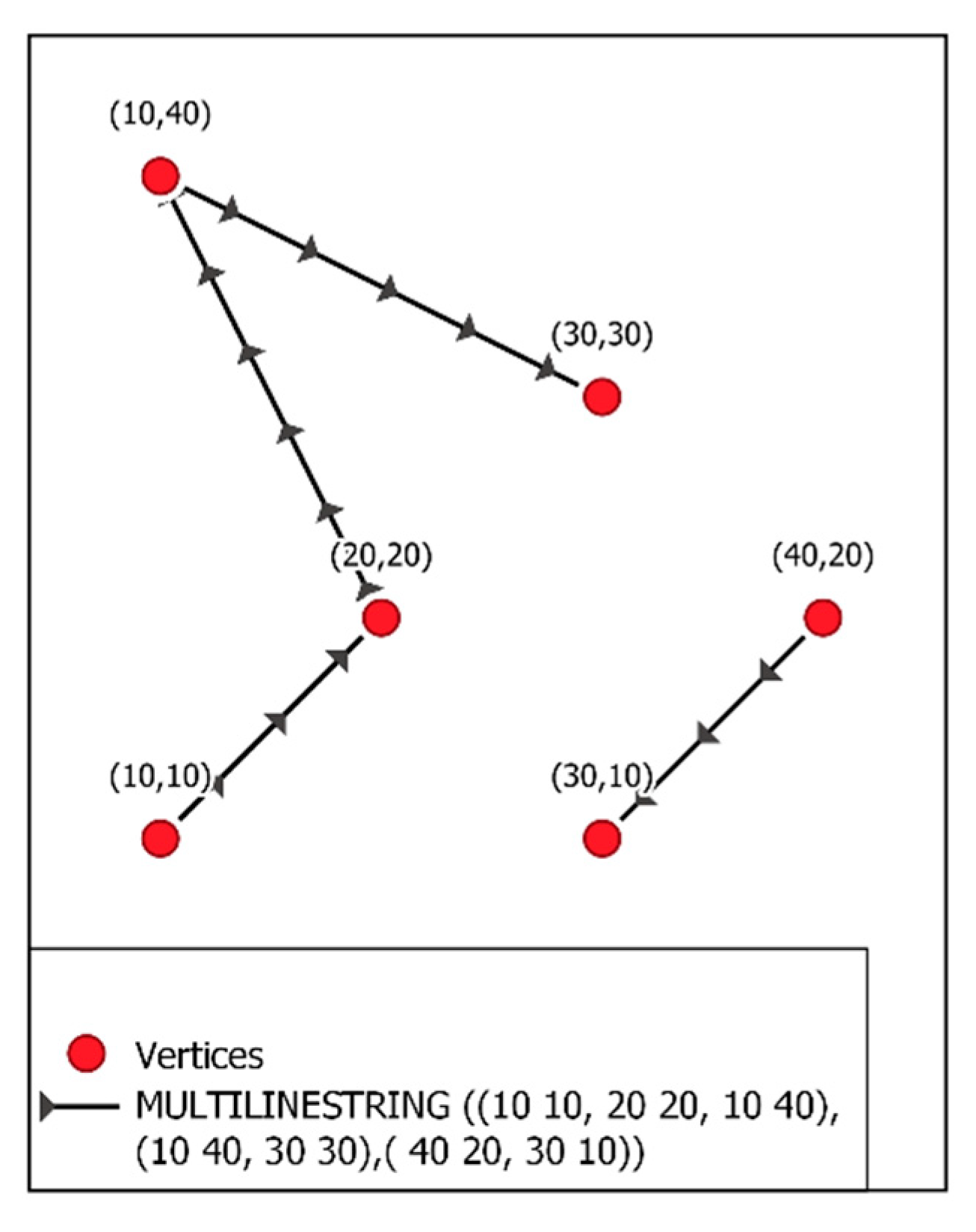
• MultiLineStrings need to be converted to LineStrings.
• LineString first or last vertex must snap (have identical coordinates) with the next object’s first or last vertex if they represent the same physical entity (river, lake…) or two physical entities that are connected. No error tolerance is built in the software.
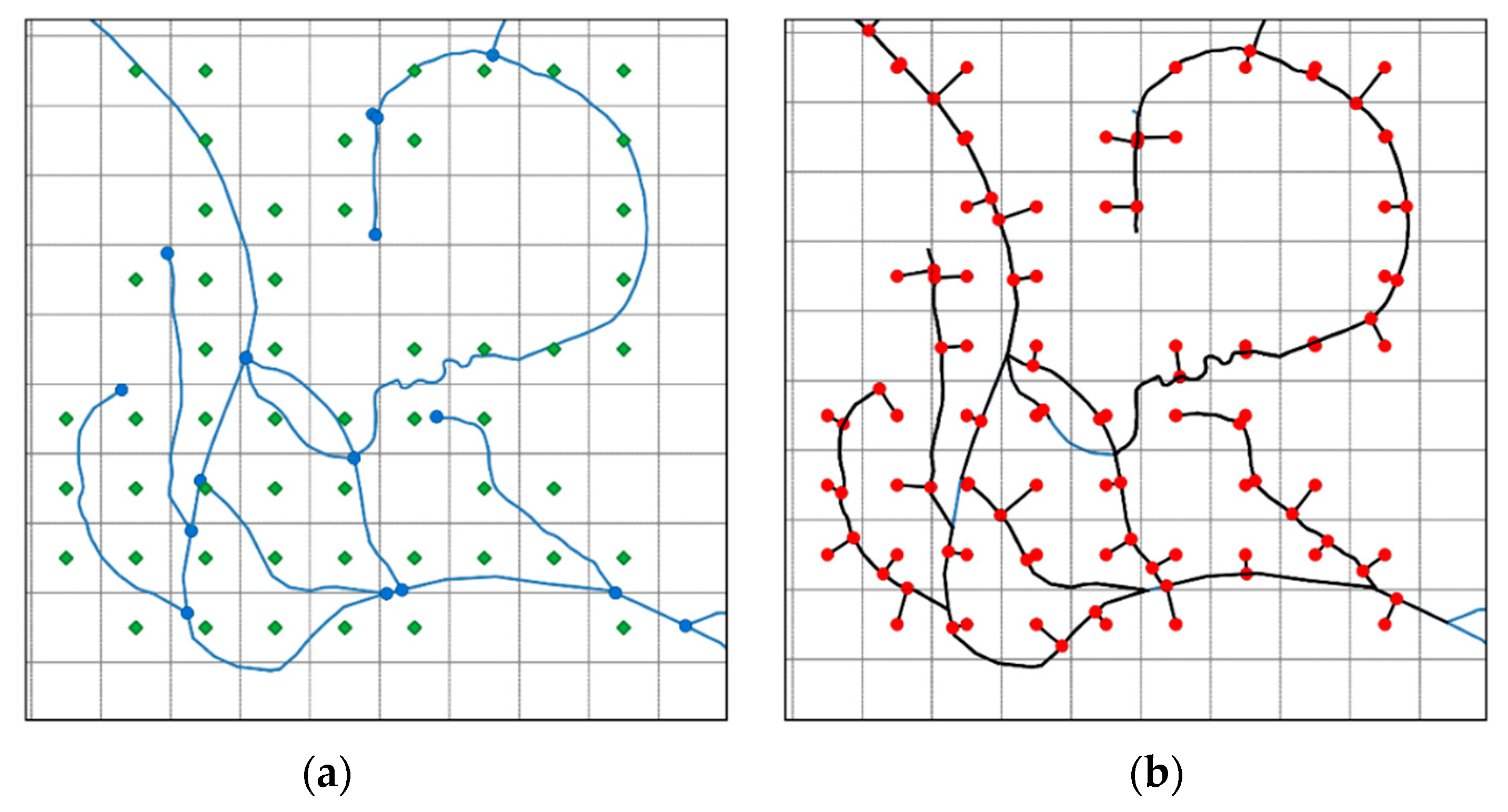
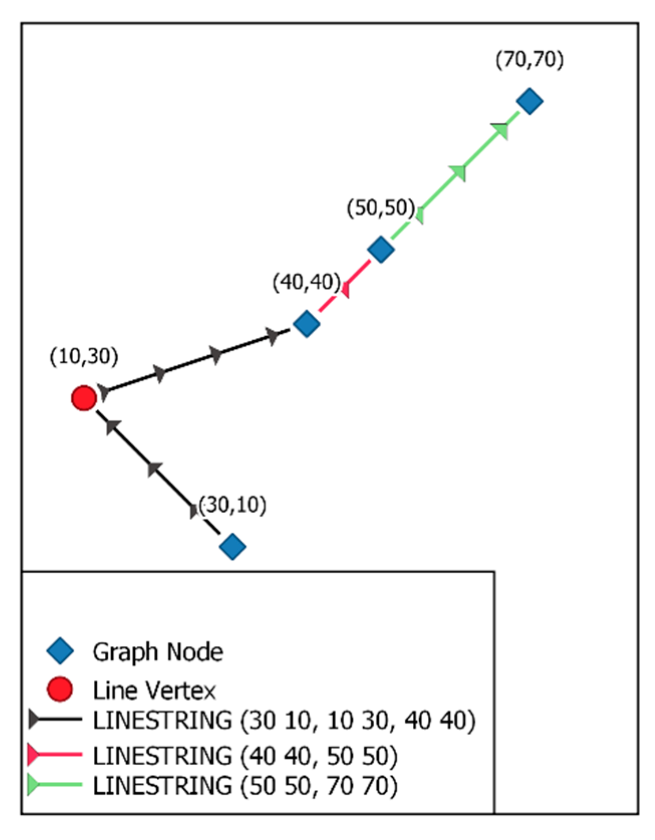
• Lines must all be vectorized from upstream to downstream. When topography is complex, this can be facilitated by draping the two-dimensional (2D) shapefile on a DEM, such as the NASA DEMs (latest SRTMs) [31]. This adds the altitude value to the Z value for each lineString vertex. LineStrings can be automatically flipped (or reversed) if the last vertex Z is higher than the first vertex Z (vectorized going upstream). All of the lines must still be manually checked for errors and most GIS packages offer lineString reversal tools. In most GIS software, line direction can be visualized by adding a simple marker (like a triangle) to the line style. The triangle can be pointed in the vectorized direction. Every line’s last vertex needs to be snapped to the next line’s first vertex. If this is not the case, then it is assumed that the end of a stream has been reached, the water flow is reversed, or there is an error in the vectorization direction.
• Most importantly, users have a tendency to vectorize single entities while using a single line object (one road = one line) (or polygon) and to snap lines using middle vertices. This simplifies the database and the drawings. However, for a graph network analysis, the lines must be broken (or split) at each intersection and snapped to all other lines in that intersection. Tools, like “planarized” in ESRI ArcGIS or “v.clean” (break, snap) in QGIS, can help. In some cases, network segment areas also split where there is no intersection. Manipulations, like dissolve and merge, followed by a multipart to single part transformation, will reduce unnecessary splitting, but will, in the process, destroy the database. These manipulations may, in return, reduce the processing time if the GIS network is unnecessarily complex.

3. Methods and Implementation

3.1. Program Overview

The following is a brief explanation of the steps that were performed by the upstream_downstream_shortests_path_dijkstra.py program. The program is downloaded as a Python source code without a graphic user interface (GUI). Functions (e.g., create_directory()) can, therefore, be directly inspected in the source code.

• Package are imported
• User Input variables are defined
• Functions are defined
• Output directories are created. See create_directory() function.
• GeoPandas reads the input network shapefile using the read_shape_file_to_gpd_df() function.
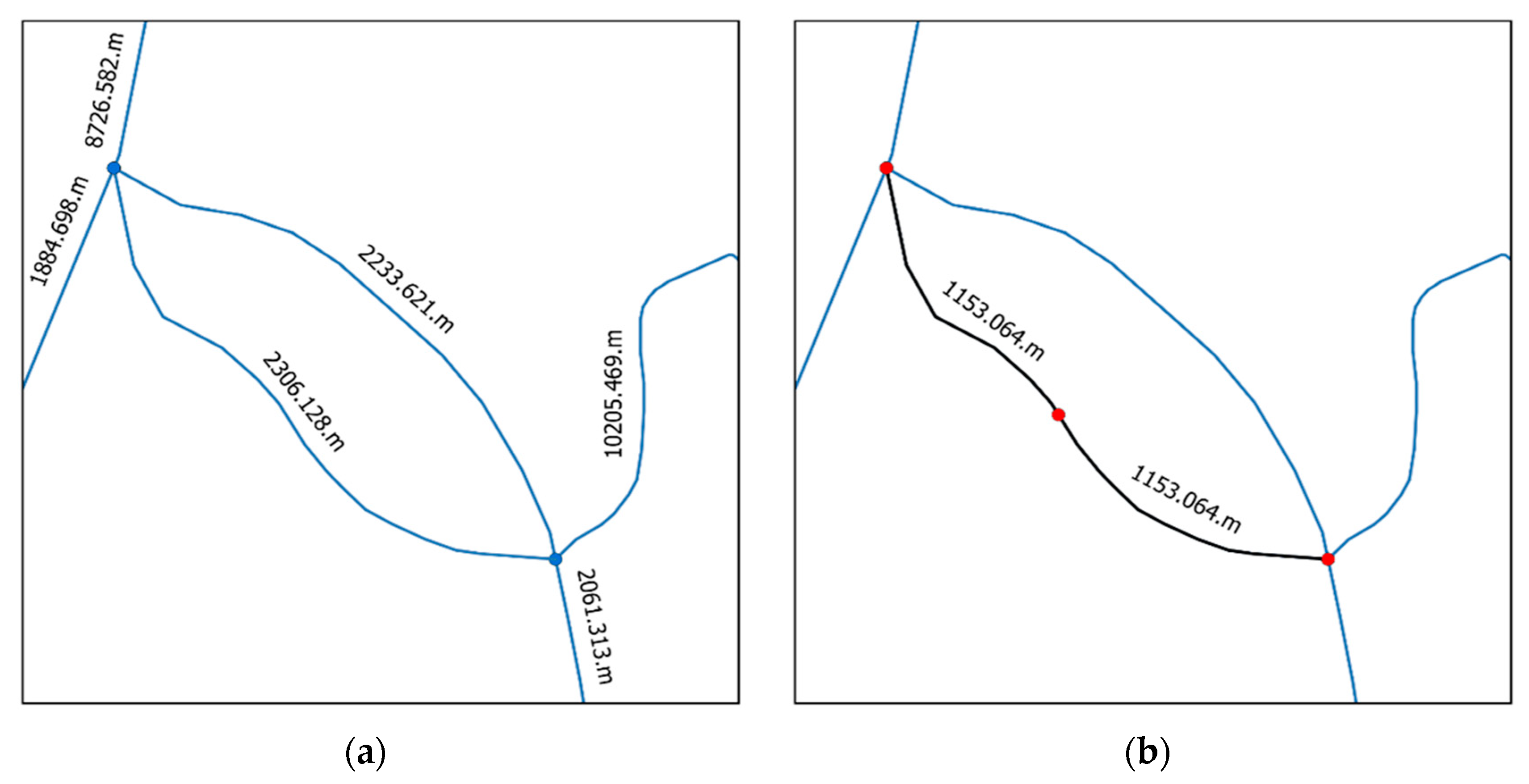
• NetworkX creates a DiGraph and the Graph with the GeoPandas DataFrame. See make_graph_from_gpd_df(). This function also creates a new GeoPandas DataFrame with parallel edges split in two as shown in Figure 2.
• Create a GeoPandas DataFrame for the input nodes using the read_shape_file_to_gpd_df() function.
• Create a Python dictionary called NEW_EDGES_DCT that contains the new nodes and the new edges that will be added on the fly to the graph (Figure 3). The cartesian length of the line geometry found in the edge attribute is used to determine the length ratio of each segment if a river lineString must be split by the algorithm. This measure is planimetric in the spatial reference system (SRS) of this geometry, but it does not consider the ellipsoid. This ratio is then applied to the user’s given unit. If river line ab is split in two segments, ab1 and ab2, the “user” length of ab1 will be calculated with the Equation (1):

  User length ab₁ = (planimetric length ab₁/(planimetric length ab₁ + planimetric length ab₂)) * user length ab

  (1)
  The tie_outside_node() function might take a long time to calculate, as it is not multithreaded. Python dictionaries can be saved to a file using the pickle_to_file() function.
• Checks the integrity between the network and graph and saves the graph to a file. Users can compare the Shapely python objects in a GIS: check_network_graph() function.
• Checks the integrity of the new nodes and new edges, saves these nodes and edges to a file. Users can compare in a GIS: save_new_edges_dct_to_csv() function.
• Makes an input list of all possible sources to target routes combinations (upper matrix only): upper_distance_matrix_route() function.
• List can be saved to file for inspection with pickle_to_file() function.
• The list from step 12 is split into chunks (according to the N_POINTS variable) and sent to the Python workers (threads)
• Sets up a pool of Python worker processes (multiprocessing threads).
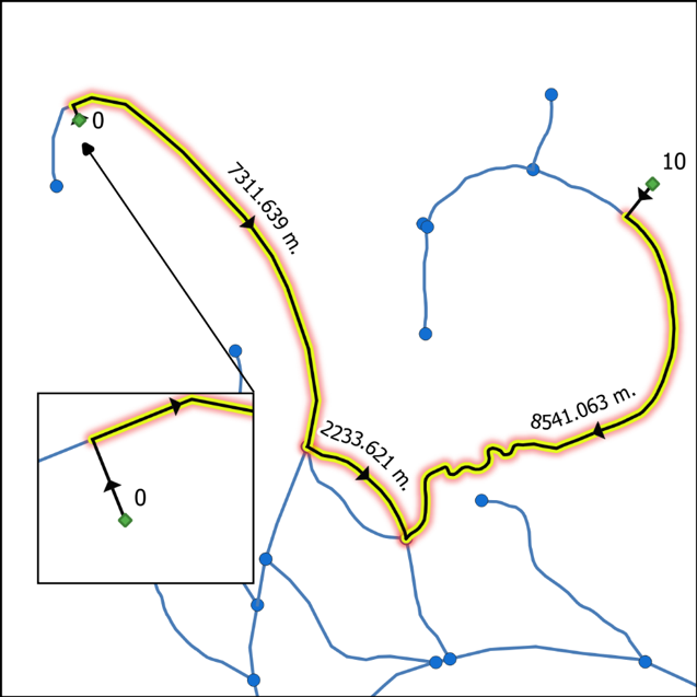
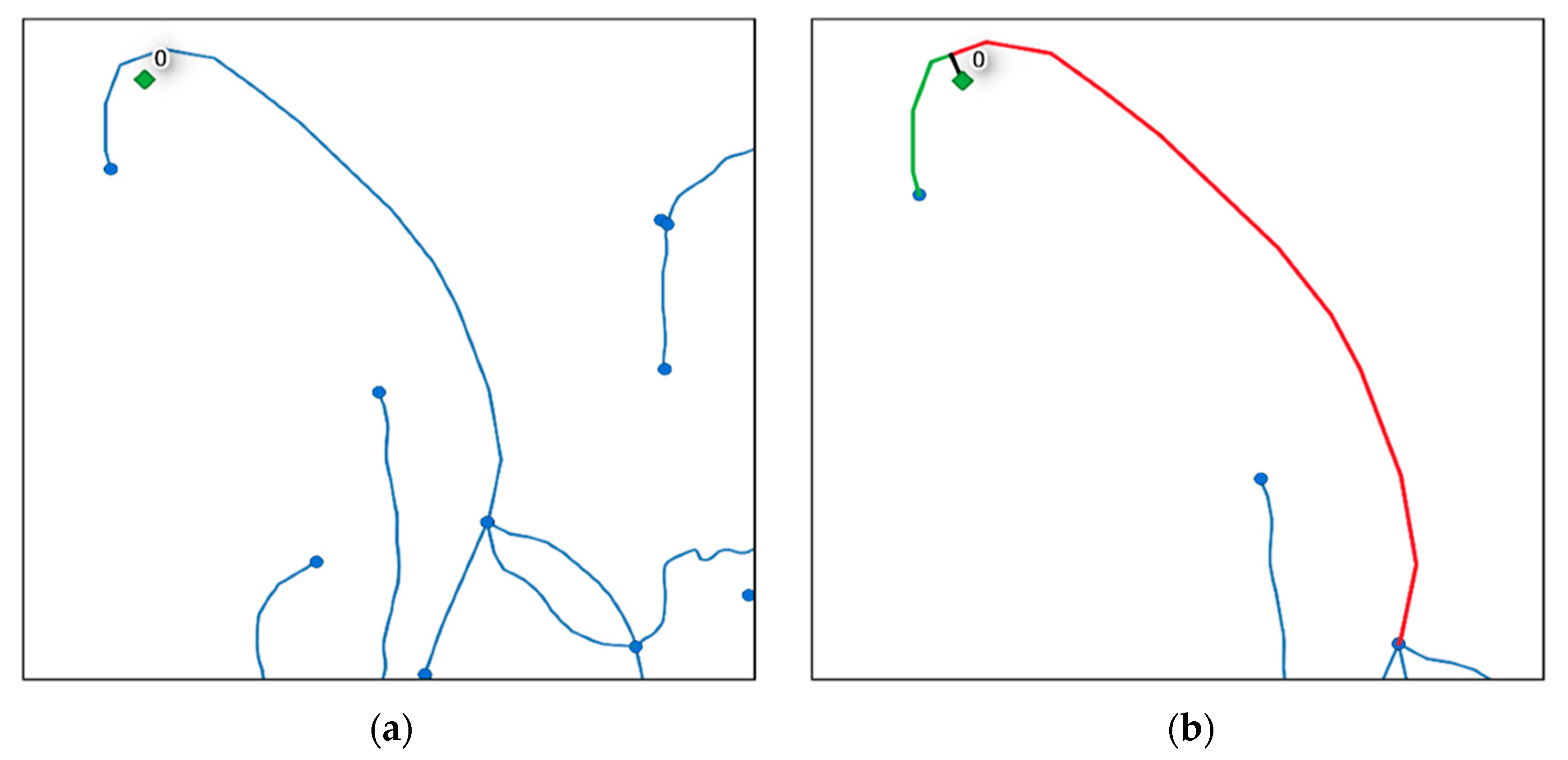
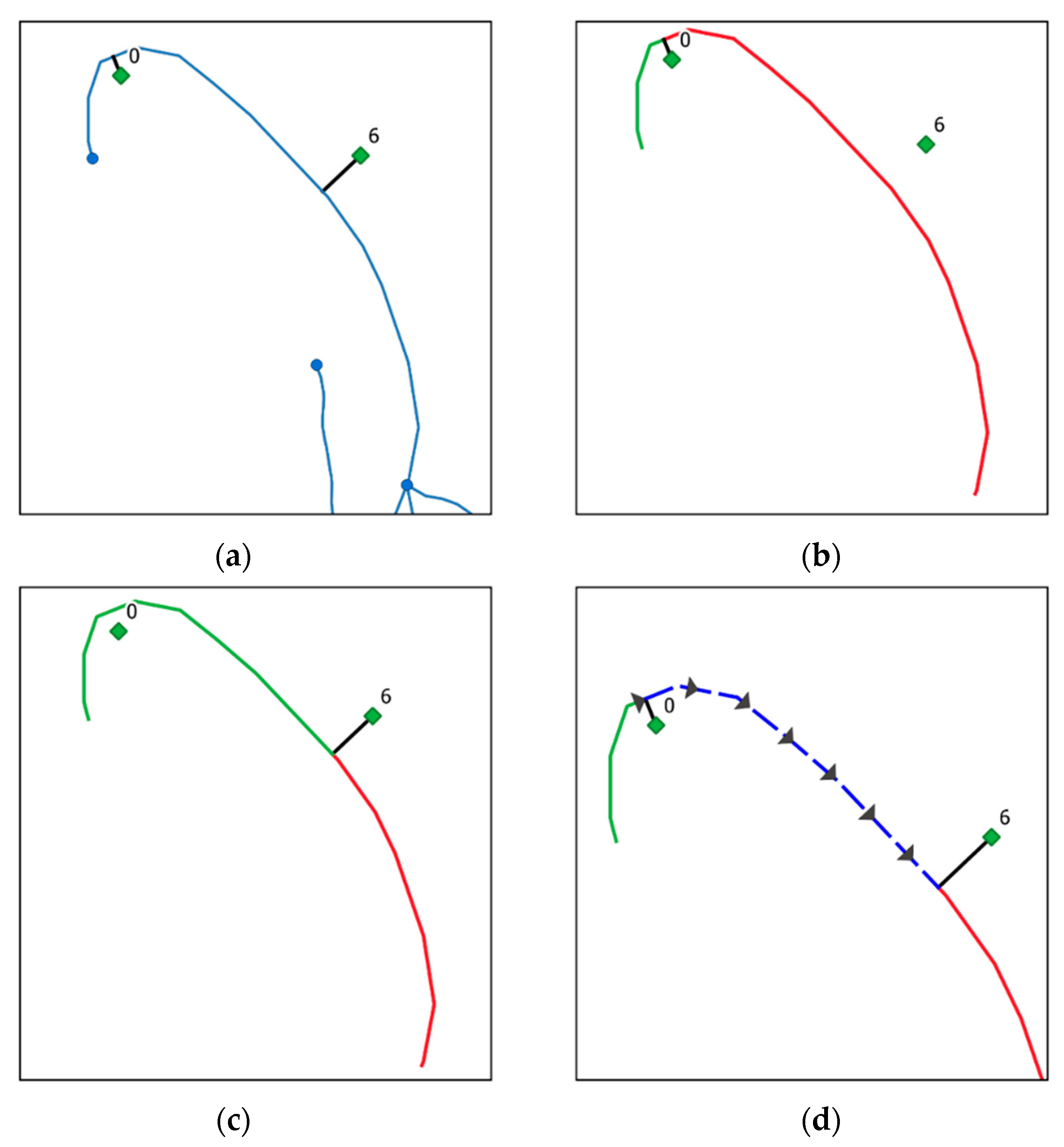
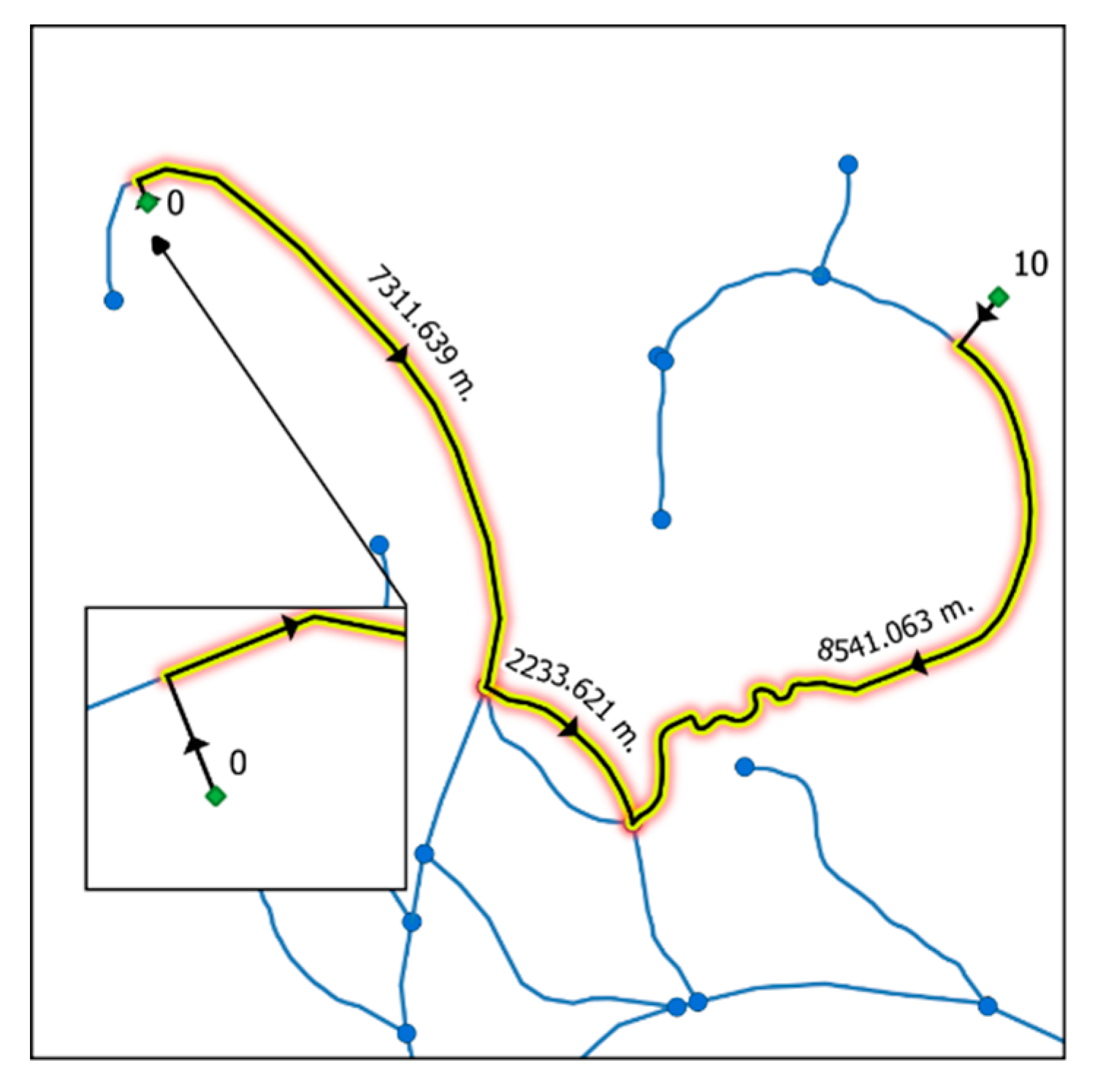
• Sends the list of routes to be calculated in chunks to a pool of workers while using the calculate_routes() function. When a route between a source node and target node is to be calculated, the first check to be done is to look up the NEW_EDGES_DCT dictionary to see if both CEs are connected to the same river segment (Figure 4a). A second verification is done to see whether the river segment is split twice by both CEs. If so, the river segment that is found between both CEs is re-split. Flow direction and total distance traveled are calculated without using the graphs (Figure 4). In all other cases, the source node and target node are inserted into the digraph and undirected graph along with accompanying edges (CEs and edges 0 and 1). The dijkstra_path (graph, source, target, [weight]) function is called and a shortest path is found. The algorithm returns a list of traveled nodes. The shortest path is calculated while using the undirected graph (Graph), while the directed graph (DiGraph) is only queried to see whether an edge is oriented downstream. As an example, if a river segment in edge (0,6) was vectorized from node 0 toward node 6, then edge (0,6) will be found in the DiGraph, but not edge (6,0). Therefore, if a route travels from node 6 to node 0, the traveler is moving upstream. Finally, each edge in the route is queried for its river flow direction and the distances are added to the upstream or downstream total distance. Before calculating the next route, all of the added edges and nodes are removed from the graphs.
  Optionally, the results can include the well-known-text geometry collection of the traveled route. As can be seen in Figure 5, this collection retains the vectorization directions of each line. Splitting the geometry from multiLineString to multiple lineStrings will permit a user to have access to individual features. The route contains the lines that are used to connect the source and target nodes to the GIS network. However, as can be seen in Figure 5, CEs are not used when calculating the distances. Only river distances are calculated.
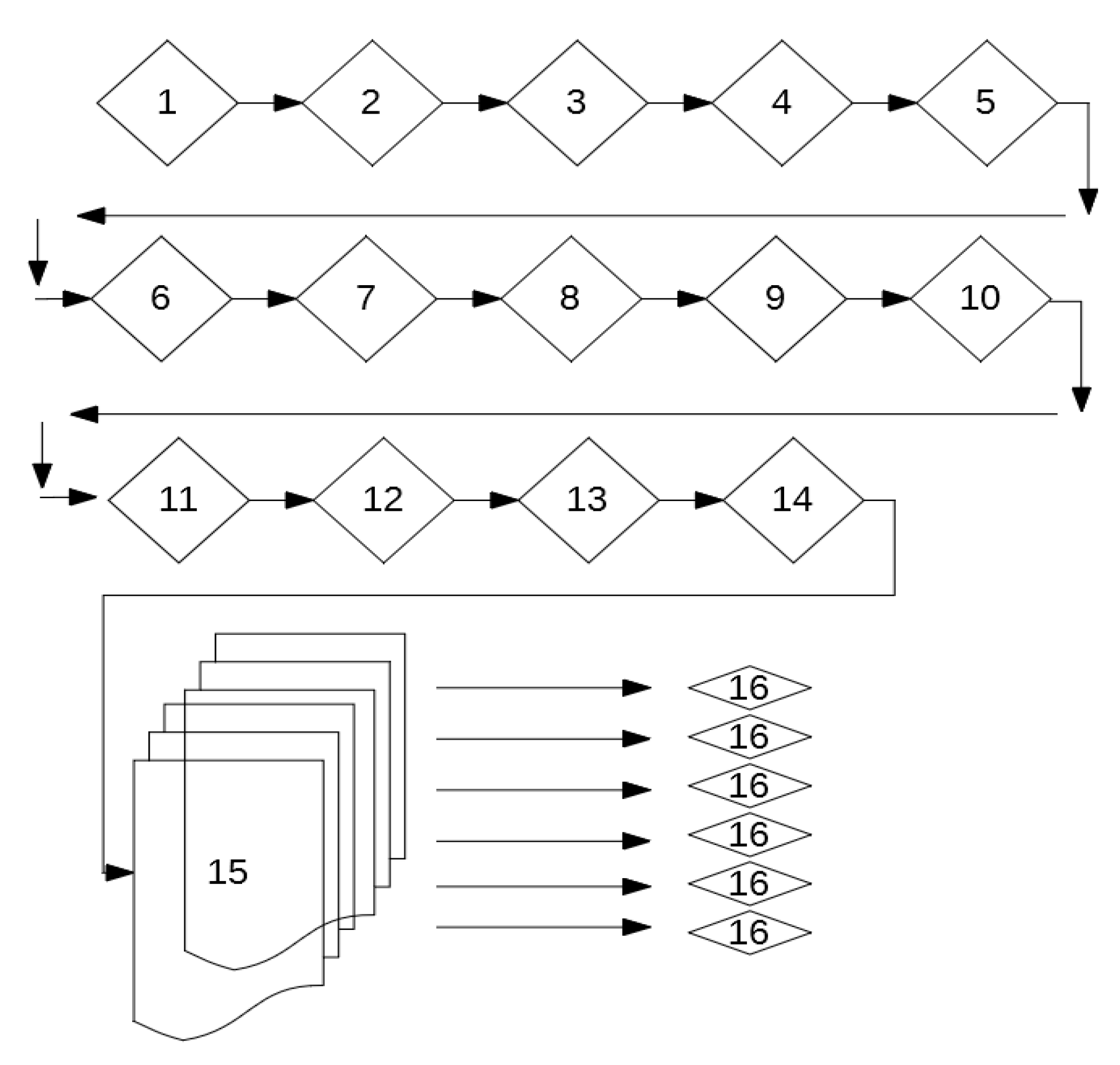
• Each worker (thread) independently saves its own file results. Steps 15 and 16 are multithreaded, as can be seen in Figure 6.

3.2. Implementation Example

Table 1. Summary of calculations carried out for four river basins in Peru. The program was implemented on a desktop system with a 6 core CPU (i7-6800K @ 3.4 GHz) (6 physical, 12 virtual cores), 64 GB of RAM and a M.2 solid state hard drive. User Input Variables were set to: THREADS = 10, N_POINTS = 1,000,000, ROUTE_RESULT_DCT_MAX_SIZE = 10,000 and INCLUDE_WKT_IN_ROUTES = False.

Basin Name	No. Graph Edges	No. Graph Nodes	No. Shortest Paths Calculated	Processing Time (min)	No. Shortest Paths/Minute
Napo	4413	3978	134,783,571	5272	25,566
Upper Ucayali	4025	3832	115,254,153	3686	31,268
Pastaza	2605	2279	28,346,685	646	43,880
Lower Ucayali	1470	1329	28,527,681	336	84,904

lists details regarding calculations that were carried out in four river basins in Peru. In contrast, attempting similar calculations with the standard QGIS options resulted in ~4 shortest paths calculated per minute.

4. User Notes

4.1. Important Vocabulary and Concepts

In a GIS, a lineString (or line) can be represented, as follows, while using the well-known text (wkt) convention for geometric objects [32] (Figure 7). The LINESTRING (30 10, 10 30, 40 40) has three vertices that are represented by coordinates (30,10), (10,30), and (40,40). The first vertex is situated at the coordinates (30,10) and the last vertex at coordinates (40,40). The river flow direction is assumed to be from the first vertex to the last vertex. Any vertex that is not a first or last vertex is referred to as a middle vertex. The first and last vertices will become nodes in graph theory. In NetworkX, nodes that are made from vector line files are named after the coordinates of the first or last nodes. A GIS vector network should be composed of lineStrings that represent physical entities, such as rivers and streams, or the centerline of river and lake polygons.

A lineString is distinct from a multiLineString (also referred to as line collection). A multiLineString might be represented, as follows (Figure 8): MULTILINESTRING ((10 10, 20 20, 10 40), (10 40, 30 30), (40 20, 30 10)). A multiLineString might (or may not) appear as a single line in a GIS. In Figure 8, it is a collection of three lines whose coordinates are grouped by the inner round brackets. multiLineStrings need to be converted to lineStrings for most GIS network analyses, because a multiLineString may represent multiple disconnected lines. These same concepts apply to points and multiPoints.

4.2. Creating a Graph with Geometric (Vector) Objects

The NetworkX python library uses graph theory in order to resolve the shortest path problem [25,33,34]. Therefore, the GIS vector network must be represented as a graph; a data structure intended to represent all of the possible connections between the objects (i.e., river segments). In a graph (G), nodes (N) will be the first or last vertex of a line and sets of nodes will become edges (E) (Figure 9).

When representing a river network in a graph, if one makes a graph with LINESTRING(30 10, 10 30, 40 40), then the graphs will be comprised of the edge E((30,10), (40,40)), named after the first and last vertices of the line. The graph will also have two nodes, N(30,10) and N(40,40) (Figure 9). All middle vertices (e.g., (10,30)) are dropped in the graph. If one adds LINESTRING(40 40, 50 50) to the graph, then E((30,10), (40,40)) will be connected to E((40,40), (50,50)) through N(40,40). N(50,50) will also be added to the graph automatically. One can add N(70, 70) to the graph without adding an edge. In this case, the node will not be connected, and no shortest path routes can be calculated to and from this node, unless it is tied to the graph with an edge. Adding a connection edge E((50,50), (70,70)) would connect the latest node to the graph.

Dijkstra’s shortest path algorithm might be implemented by finding the route that travels the fewest number of nodes. Here, the shortest path is calculated while using a weight (i.e., distance) that was attributed to the edge. In NetworkX, any python object can also be used as an edge attribute and we, therefore, take advantage of the Python Shapely library [35]. In this case, the river length and the Python Shapely object (the geometric line) are included in the edge attributes.

4.3. Setting Up the Python Environment

Users will need the following packages installed. The package versions indicate the development setup while using the Anaconda Python Distribution [10]. The packages may be installed via the Anaconda Navigator, conda install or pip commands.

• Pandas (0.24.2)
• Geopandas (0.4.1)
• NetworkX (2.3)
• Shapely (1.6.4)

4.4. Setting Up the User Input Variables

Users must add the following “User Input Variables” at the beginning of the script:

• INCLUDE_WKT_IN_ROUTES = False. If set to True, the program will add the nodes travelled list and well-known-text of routes in results. This will considerably slow down the program.
• BASIN = Name of the river basin. This will be used in the output file names.
• OUTPUT_FILE_MAIN_DIRECTORY = Complete path of the output file directory
• INPUT_NETWORK_FILE_SHP = Complete path for the input network.shp file
• INFILE_LENGTH = This is the name of length variable in the input network shapefile (network.shp).
• INPUT_ROUTES_SHP = Complete path to the node.shp file. This is the shapefile containing the source nodes that to be used as source and target nodes for the shortest path distances. If some of the nodes are already in the graph, they will need to be added to this file.
• THREADS = Number of Threads to be used to calculate routes (one per logical core). Keep one or two cores free.
• N_POINTS = The number of route calculations to send to each thread at a time. In order to speed up Python’s traditional slower speeds, the program is multithreaded with each thread solving a group of shortest paths (typically, one-million routes each). Output files are independently written by the threads and will contain the same number of routes.
• ROUTE_RESULT_DCT_MAX_SIZE = Number of shortest path results each thread must keep in memory before writing the results to the output files (typically 5000 to 10,000 results). A high number will increase memory usage, but decrease the number of disk writes.

5. Conclusions

Roads are often thought of as the modern topological equivalent of rivers. GIS approaches typically adhere to this over simplified view, as shortest path algorithms are designed with road networks in mind. Therefore, we have developed an OpenSource software (upstream_downstream_shortests_path_dijkstra.py) that implements an all-pairs shortest path (Dijkstra’s algorithm) on river networks that will return the total upstream and downstream distances travelled on each route. The algorithm could further be used for effectively calculating millions of routes, where traffic direction is no longer an issue (e.g., after a major disaster) or in situations where a geometric network is vectorized in a specific direction, but where bi-directional communication and circulation is allowed.

References

1. dos Santos, A.D.; Costa, L.; Braga, M.D.; Velloso, P.B.; Ghamri-Doudane, Y. Characterization of a delay and disruption tolerant network in the Amazon basin. Veh. Commun. 2016, 5, 35–43. [Google Scholar] [CrossRef]
2. Salonen, M.; Toivonen, T.; Cohalan, J.M.; Coomes, O.T. Critical distances: Comparing measures of spatial accessibility in the riverine landscapes of Peruvian Amazonia. Appl. Geogr. 2012, 32, 501–513. [Google Scholar] [CrossRef]
3. Tenkanen, H.; Salonen, M.; Lattu, M.; Toivonen, T. Seasonal fluctuation of riverine navigation and accessibility in Western Amazonia: An analysis combining a cost-efficient GPS-based observation system and interviews. Appl. Geogr. 2015, 63, 273–282. [Google Scholar] [CrossRef] [Green Version]
4. Coomes, O.T.; Takasaki, Y.; Abizaid, C.; Arroyo-Mora, J.P. Environmental and market determinants of economic orientation among rain forest communities: Evidence from a large-scale survey in western Amazonia. Ecol. Econ. 2016, 129, 260–271. [Google Scholar] [CrossRef]
5. Guagliardo, S.A.; Morrison, A.C.; Barboza, J.L.; Requena, E.; Astete, H.; Vazquez-Prokopec, G.; Kitron, U. River Boats Contribute to the Regional Spread of the Dengue Vector Aedes aegypti in the Peruvian Amazon. PLoS Negl. Trop. Dis. 2015, 9. [Google Scholar] [CrossRef] [PubMed]
6. Parry, L.; Peres, C.A. Evaluating the use of local ecological knowledge to monitor hunted tropical-forest wildlife over large spatial scales. Ecol. Soc. 2015, 20. [Google Scholar] [CrossRef] [Green Version]
7. Tregidgo, D.J.; Barlow, J.; Pompeu, P.S.; Rocha, M.D.; Parry, L. Rainforest metropolis casts 1,000-km defaunation shadow. Proc. Natl. Acad. Sci. USA 2017, 114, 8655–8659. [Google Scholar] [CrossRef] [Green Version]
8. Apolinaire, E.; Bastourre, L. Nets and canoes: A network approach to the pre-Hispanic settlement system in the Upper Delta of the Parana River (Argentina). J. Anthropol. Archaeol. 2016, 44, 56–68. [Google Scholar] [CrossRef]
9. Arias, L.; Barbieri, C.; Barreto, G.; Stoneking, M.; Pakendorf, B. High-resolution mitochondrial DNA analysis sheds light on human diversity, cultural interactions, and population mobility in Northwestern Amazonia. Am. J. Phys. Anthropol. 2018, 165, 238–255. [Google Scholar] [CrossRef]
10. Ranacher, P.; van Gijin, R.; Derungs, C. Identifying probable pathways of language diffusion in South America. In Proceedings of the AGILE conference Wageningen, Wageningen, The Netherlands, 9–12 May 2017. [Google Scholar]
11. Schillinger, K.; Lycett, S.J. The Flow of Culture: Assessing the Role of Rivers in the Inter-community Transmission of Material Traditions in the Upper Amazon. J. Archaeol. Method Theory 2019, 26, 135–154. [Google Scholar] [CrossRef]
12. Loidl, M.; Wallentin, G.; Cyganski, R.; Graser, A.; Scholz, J.; Haslauer, E. GIS and Transport Modeling-Strengthening the Spatial Perspective. ISPRS Int. J. Geo-Inf. 2016, 5, 84. [Google Scholar] [CrossRef] [Green Version]
13. Obe, R.O.; Hsu, L.S.; Sherman, G.E. PgRouting: A Practical Guide; Locate Press: Chugiak, AK, USA, 2017. [Google Scholar]
14. Yang, C.W.; Raskin, R.; Goodchild, M.; Gahegan, M. Geospatial Cyberinfrastructure: Past, present and future. Comput. Environ. Urban Syst. 2010, 34, 264–277. [Google Scholar] [CrossRef]
15. Nasri, M.I.; Bektas, T.; Laporte, G. Route and speed optimization for autonomous trucks. Comput. Oper. Res. 2018, 100, 89–101. [Google Scholar] [CrossRef] [Green Version]
16. Schroder, M.; Cabral, P. Eco-friendly 3D-Routing: A GIS based 3D-Routing-Model to estimate and reduce CO2-emissions of distribution transports. Comput. Environ. Urban Syst. 2019, 73, 40–55. [Google Scholar] [CrossRef] [Green Version]
17. Zeng, W.L.; Miwa, T.; Morikawa, T. Application of the support vector machine and heuristic k-shortest path algorithm to determine the most eco-friendly path with a travel time constraint. Transp. Res. Part D-Transp. Environ. 2017, 57, 458–473. [Google Scholar] [CrossRef]
18. NetworkX. Software for Complex Networks. Available online: https://networkx.github.io (accessed on 9 November 2019).
19. Dijkstra, E.W. A note on two problems in connection with graphs. Numer. Math. 1959, 1, 269–271. [Google Scholar] [CrossRef] [Green Version]
20. Gallo, G.; Pallottino, S. Shortest Path Algorithms. Ann. Oper. Res. 1988, 13, 1–79. [Google Scholar] [CrossRef]
21. Ford, L.R., Jr. Network Flow Theory; The RAND Corporation: Santa Monica, CA, USA, 1956. [Google Scholar]
22. Johnson, D.B. Efficient Algorithms for Shortest Paths in Sparse Networks. J. Assoc. Comput. Mach. 1977, 24, 1–13. [Google Scholar] [CrossRef]
23. Floyd, R.W. Algorithm 97: Shortest Path. Commun. ACM 1962, 5, 345. [Google Scholar] [CrossRef]
24. Ortega-Arranz, H.; Llanos, D.R.; Gonzalez-Escribano, A. The shortest-path problem. In Analysis and Comparison of Methods; Morgan&Claypool Publishers: San Rafael, CA, USA, 2015. [Google Scholar]
25. Hart, E.P.; Nilsson, N.J.; Raphael, B. A formal basis for the heuristic determination of minimum cost paths. IEEE Trans. Syst. Sci. Cybern. 1968, 4, 100–107. [Google Scholar] [CrossRef]
26. Telles, M. Python Power: The Comprehensive Guide; Thomson Course Technology: Boston, MA, USA, 2008. [Google Scholar]
27. Muller, M.; Bernard, L.; Kadner, D. Moving code—Sharing geoprocessing logic on the Web. ISPRS J. Photogramm. Remote Sens. 2013, 83, 193–203. [Google Scholar] [CrossRef]
28. Scheider, S.; Ballatore, A.; Lemmens, R. Finding and sharing GIS methods based on the questions they answer. Int. J. Digit. Earth 2019, 12, 594–613. [Google Scholar] [CrossRef] [Green Version]
29. GeoPandas. Available online: http://geopandas.org (accessed on 9 November 2019).
30. ESRI. ESRI Shapefile Technical Description an ESRI White Paper; ESRI: Redlands, CA, USA, 1998. [Google Scholar]
31. Crippen, R.; Buckley, S.; Agram, P.; Belz, E.; Gurrola, E.; Hensley, S.; Kobrick, M.; Lavalle, M.; Martin, J.; Neumann, M.; et al. NASADEM Global Elevation Model: Methods and Progress. In XXIII ISPRS Congress, Commission IV; International Archives of the Photogrammetry Remote Sensing and Spatial Information Sciences; Halounova, L., Safar, V., Jiang, J., Olesovska, H., Dvoracek, P., Holland, D., Seredovich, V.A., Eds.; Copernicus Gesellschaft Mbh: Gottingen, Germany, 2016; pp. 125–128. [Google Scholar]
32. Open Geospatial Consortium Inc. OpenGIS® Implementation Standard for Geographic Information—Simple Feature Access—Part 1: Common Architecture; Herring, J.R., Ed.; Open Geospatial Consortium Inc.: Wayland, MA, USA, 2011. [Google Scholar]
33. Boeing, G. OSMnx: New methods for acquiring, constructing, analyzing, and visualizing complex street networks. Comput. Environ. Urban Syst. 2017, 65, 126–139. [Google Scholar] [CrossRef] [Green Version]
34. Harary, F. Graph Theory; Addison-Wesley Publishing Co.: Reading, CA, USA, 1969. [Google Scholar]
35. Toblerity/Shapely. Available online: https://github.com/Toblerity/Shapely (accessed on 9 November 2019).
Figure 1. (a) The original simpler geographic information system (GIS) river network. Blue vertices will become nodes in the graph. Source and target nodes for the shortest path algorithm are in green. Here, source and target nodes are grid centroids situated at a maximum of 1000 m from the river. (b) New edges are in black and new nodes are in red. The few remaining blue edges in (b) (near the center and lower right portions of (b)) indicate the areas where new edges are not needed for the algorithm to work.
Data 05 00008 g001
Figure 2. (a) The original GIS network with two parallel channels. Both river channels are connected to the same nodes (blue points). In (b), the lower channel has been split in two segments (in black) in order to avoid parallel edges in the graph. Original user line length in (a) is 2306.128 m, in (b) the weight has been divided by 2 (1153.064 m).
Data 05 00008 g002
Figure 3. Adding a new node to the graph. (a) Node 0 (green square) is not connected to the graph. In (b), a connection edge (CE) (black line) is created by forming a line between a source or target node and the closest point found on the closest geometry. If this node is not already present in the graph network, and then the nearest river segment is split in two geometries (green and red lines). The new nodes, edges, edge length, or weight are recalculated. The Shapely geometries are then stored in the python dictionary. New nodes, edges, recalculated weights and geometries are stored in the NEW_EDGES_DCT variable (a Python dictionary).
Data 05 00008 g003
Figure 4. (a) Both nodes 0 and 6 are connected to the same river segment. Node 0, its CE (black) and the split river segments (red and green) are stored in the dictionary (b). Node 6, its CE (black) and the split river segments (red line and green line) are stored in the dictionary (c). Solution for the shortest path is found by re-splitting the red geometry from (b) with the CE geometry of node 6 (black line in c). The result is the blue dash line shown in (d). As no other path exists, there is no need to use the Dijkstra algorithm in this case.
Data 05 00008 g004
Figure 5. Optional output of the well-known-text multiLineString route of the shortest path between source node 0 and target node 10. Yellow highlight indicates what parts of the routes are used when measuring the total distances travelled (CE geometries are excluded). When converted to multiple LineStrings, the direction of the current (black triangles) and the length of each segment can be easily inspected in a GIS.
Data 05 00008 g005
Figure 6. Basic schema for the software. The numbers represent the steps described above.
Data 05 00008 g006
Figure 7. Well-known-text and geometric representation of a lineString. Arrows on the line represent the vectorization (river current) direction.
Data 05 00008 g007
Figure 8. Well-known-text and geometric representation of a multiLineString. Here it is composed of three lineStrings although we perceive only two objects. A multiLineString is considered as a single object by most GIS software and is generally linked to a single database entry. Arrows on the lines represent the vectorization (river current) direction.
Data 05 00008 g008
Figure 9. Adding nodes (N) and edges (E) to a graph. N(70,70) is connected to the graph with E((50,50),(70,70)).
Data 05 00008 g009