Information Loss Due to the Data Reduction of Sample Data from Discrete Distributions

Abstract

In this paper, we study the information lost when a real-valued statistic is used to reduce or summarize sample data from a discrete random variable with a one-dimensional parameter. We compare the probability that a random sample gives a particular data set to the probability of the statistic’s value for this data set. We focus on sufficient statistics for the parameter of interest and develop a general formula independent of the parameter for the Shannon information lost when a data sample is reduced to such a summary statistic. We also develop a measure of entropy for this lost information that depends only on the real-valued statistic but neither the parameter nor the data. Our approach would also work for non-sufficient statistics, but the lost information and associated entropy would involve the parameter. The method is applied to three well-known discrete distributions to illustrate its implementation.

1. Introduction

We consider the data sample $x=\left({\mathrm{x}}_1, \dots ,{ \mathrm{x}}_{\mathrm{n}}\right)$ from a random sample $X=\left({\mathrm{X}}_1, \dots ,{ \mathrm{X}}_{\mathrm{n}}\right)$ for a discrete random variable $\mathrm{X}$ with sample space $\mathrm{S}$ and one-dimensional parameter $\mathsf{\theta }.$ A statistic $\mathrm{T}\left(X\right)$ is a function of the random sample $X$ for any fixed but arbitrary value of a parameter $\mathsf{\theta }$ associated with the underlying $\mathrm{X}.$ Thus a statistic $\mathrm{T}\left(X\right)$ is a random variable itself. Here we consider only real-valued statistics that reduce the data sample $x$ to a number $\mathrm{T}\left(x\right)$ that might be used to summarize $X,$ to characteriz $\mathrm{X}$, $\mathrm{or} \mathrm{perhaps} \mathrm{to} \mathrm{estimate} \mathsf{\theta }.$ However, data reduction is an irreversible process [1] and always involves some information loss. For instance, if $\mathrm{T}\left(X\right)$ is the sample mean $\overline{\mathrm{X}},$ the original measurements $x$ cannot be reconstructed from $\overline{\mathrm{x}},$ and some information about $x$ is lost. Nonetheless, such data reduction is frequently used to make inferences.

More explicitly, our motivation for considering such situations is that $\mathrm{T}\left(x\right)$ is usually communicated in practice as a summary for the data $x$ but without the actual data. The question then naturally arises: how much information is lost to someone about a data sample $x$ when only the value of $\mathrm{T}$ is available for $x$, but not the data itself? To answer this question, we develop a theoretical framework for determining how much information is lost about a given data set $x$ by knowing only the value of $\mathrm{T}\left(x\right)$ but neither $x$ itself nor the parameter $\mathsf{\theta }$. Our information-theoretic approach to data reduction generalizes the observation in [2] that a binomial random variable loses all the information about the order of successes in the associated sequence of Bernoulli trials. In other words, for a series of n Bernoulli trials one cannot recreate the order of successes by only knowing the number that occurred.

For any real-valued statistic $\mathrm{T}$ and the given sample data $x,$ we decompose the total information about $X$ available in $x$ into the sum of (a) the information available in the reduced data $\mathrm{T}\left(x\right)=\overline{x}$ and (b) the information lost in the process of data reduction. When $\mathrm{T}$ is a sufficient statistic for $\mathsf{\theta },$ this lost information is independent of $\mathsf{\theta }$. Moreover, by taking the expected value of this lost information over all possible data sets, we define an associated entropy measure that depends on $\mathrm{T}$ but neither $x$ nor $\mathsf{\theta }$. Our approach also works for non-sufficient statistics, but the lost information and associated entropy would then involve $\mathsf{\theta }$. Thus $\mathsf{\theta }$ must be estimated before computing these quantities.

The paper is organized as follows. In Section 2, we present the necessary definitions, notation, and preliminary results. In Section 3, we decompose the total information available about $X$ in $x$ and give various expressions for the Shannon information lost by reducing $x$ to $\mathrm{T}\left(x\right).$ In Section 4, we develop an entropy measure associated with this lost information. In Section 5, we present examples of our results for some standard discrete distributions and several sufficient statistics for $\mathsf{\theta }.$ Conclusions are offered in Section 6.

2. Preliminaries

Standard definitions, notation, and results to be used in our development are now presented for completeness and accessibility. In addition, some new definitions and results are established for subsequent use. Definition 1, Result 1, Definition 2, and Definition 3 can be found in [3,4,5] and elsewhere. The notion of a sufficient statistic is first defined.

Definition 1 (Sufficient Statistic [3]).

A statistic$T\left(X\right)$is a sufficient statistic (SS) for the parameter$\theta$if the probability

$$\mathrm{P}[X=x|\mathrm{T}\left(X\right)=\mathrm{T}\left(x\right)]$$

(1)

is independent of$\theta$.

Note that $\mathrm{P}$ instead of ${\mathrm{P}}_{\mathsf{\theta }}$ is used in (1) since this probability is independent of $\mathsf{\theta }.$ In addition, observe that (1) is not a joint conditional probability distribution for $X$ since its condition changes with $x$. This observation is significant in Section 4. The fact that (1) does not involve $\mathsf{\theta }$ can be used to prove the Fisher Factorization Theorem (FFT) below, which is the usual method for determining if a statistic is an SS for $\mathsf{\theta }$. In the FFT, we use the notation $\mathrm{f}(x|\mathsf{\theta })$ to denote the joint probability mass function (pmf) of $X$ evaluated at the variable $x$ for a fixed value of $\mathsf{\theta }$.

Result 1 (FFT [3]).

The real-valued statistic$T\left(X\right)$is sufficient for$\theta$if and only if there exist functions$g:R^1\to R^1$and$h:S^n\to R^1$such that for any sample data$x$and for all values of$\theta$the joint pmf$f(x|\theta )$of$X$can be factored as

$$\mathrm{f}\left(x|\mathsf{\theta }\right)=\mathrm{g}\left[\mathrm{T}\left(x\right)|\mathsf{\theta }\right]\times \mathrm{h}\left(x\right)$$

(2)

for real-valued, nonnegative functions$g$on and$h$on$S^n.$The function$h$does not depend on$\theta ,$while$g$does depend on$x$but only through$T\left(x\right).$

We focus on a sufficient statistic $\mathrm{T}$ for $\mathsf{\theta }$ in Section 3, where we need the notion of a partition [5] defined next.

Definition 2 (Partition [3]).

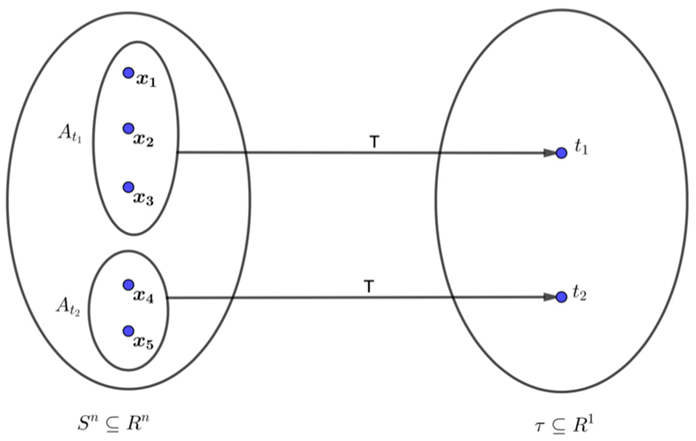
Let$S$be the denumerable sample space of the discrete random variable$X$so that$S^n$is the denumerable sample space of the random sample$X$. For any statistic$T:S^n\to R^1$, let${\tau }_T$be the denumerable set${\tau }_T=\left\{t\right|\exists x\in S^n$for which$t=T\left(x\right)\}$, which is the range of$T.$Then$T$partitions the sample space$S^n$into the mutually exclusive and collectively exhaustive partition sets$A_t=\left\{x\in S^n|T\left(x\right)=t\right\}, \forall t\in {\tau }_T$.

Figure 1 illustrates Definition 2.

We also use the well-known likelihood function.

Definition 3 (Likelihood Function [3,4,5]).

Let$x$be sample data from a random sample$X$from a discrete random variable$X$with sample space$S$and real-valued parameter$\theta ,$and let$f(x|\theta )$denote the joint pmf of the random sample$X$. For any sample data$x$, the likelihood function of$\theta$is defined as

$$\mathrm{L}\left(\mathsf{\theta }|x\right)=\mathrm{f}(x|\mathsf{\theta }).$$

(3)

The likelihood function $\mathrm{L}\left(\mathsf{\theta }|x\right)$ in (3) is a function of the variable $\mathsf{\theta }$ for given data $x$. However, the joint pmf $\mathrm{f}\left(x|\mathsf{\theta }\right)$ as a function of $x$ for fixed $\mathsf{\theta }$ is frequently called the likelihood function as well. In this case, we also write the joint pmf as $\mathrm{L}\left(x|\mathsf{\theta }\right).$ We distinguish the two cases since $\mathrm{L}\left(\mathsf{\theta }|x\right)$ is not a statistic but $\mathrm{L}\left(x|\mathsf{\theta }\right)$ is one that incorporates all available information about $X$. Moreover, $\mathrm{L}\left(x|\mathsf{\theta }\right)$ is an SS for $\mathsf{\theta }$ [4] and uniquely determines an associated SS called the likelihood kernel to be used in subsequent examples.

We next define a new concept called the likelihood kernel. As a function of $x$ for fixed $\mathsf{\theta }$, it is shown below to be a sufficient statistic for $\mathsf{\theta }$ and is used in Section 5 to facilitate the computation of lost information associated with other sufficient statistics T. As a function of $\mathsf{\theta }$ for fixed $x$, a possibility not considered here, the likelihood kernel may be useful in applying the likelihood principle [3,4] to make inferences about $\mathsf{\theta }$ without resorting to the notion of equivalence classes. It would be the “simplest” factor of $\mathrm{L}\left(\mathsf{\theta }|x\right)$ that can be used in a likelihood ratio comparing two values of $\mathsf{\theta }.$

Definition 4 (Likelihood kernel).

Let$S$be the sample space of$X$. For fixed but arbitrary$\theta ,$suppose that$L\left(x\right|\theta )$can be factored as

$$\mathrm{L}(x|\mathsf{\theta })=\mathrm{K}(x|\mathsf{\theta })\times \mathrm{R}\left(x\right), \forall x\in {\mathrm{S}}^{\mathrm{n}},$$

(4)

where$K:S^n\to R^1$and$R:S^n\to R^1$have the following properties.

 (a) 

Every nonnumerical factor of$K\left(\mathit{x}\right|\theta )$contains$\theta .$

 (b) 

$R\left(\mathit{x}\right)$does not contain$\theta .$

 (c) 

For$\forall \mathit{x}\in S^n,$both$K\left(\mathit{x}\right|\theta )\ge 0$and$R\left(\mathit{x}\right)\ge 0.$

 (d) 

$K\left(\mathit{x}\right|\theta )$is not divisible by any positive number except 1.

Then$K\left(\mathit{x}\right|\theta )$is defined as the likelihood kernel of$L\left(\mathit{x}\right|\theta )$and$R\left(\mathit{x}\right)$as the residue of$L\left(\mathit{x}\right|\theta ).$

Theorem 1.

The likelihood kernel$K\left(x\right|\theta )$has the following properties.

 (i) 

$K\left(\mathit{x}\right|\theta )$exists uniquely.

 (ii) 

$K\left(\mathit{x}\right|\theta )$is an SS for$\theta$.

 (iii) 

For any${\theta }_1$and${\theta }_2,$the likelihood ratio$\frac{L\left(\mathit{x}|{\theta }_1\right)}{L\left(\mathit{x}|{\theta }_2\right)}$equals$\frac{K\left(\mathit{x}|{\theta }_1\right)}{ K\left(\mathit{x}|{\theta }_2\right)}.$

 Proof. 

To prove (i), for fixed $\mathsf{\theta }$ we first show that the likelihood kernel $\mathrm{K}(x|\mathsf{\theta })$ of Definition 4 exists by construction. Since the formula for $\mathrm{L}\left(\mathsf{\theta }|x\right)=\mathrm{f}(x|\mathsf{\theta })$ must explicitly contain $\mathsf{\theta },$ the parameter $\mathsf{\theta }$ cannot appear only in the range of $x$. Hence $\mathrm{L}(x|\mathsf{\theta })$ as a function of $x$ can be factored into $\mathrm{K}(x|\mathsf{\theta })\times \mathrm{R}\left(x\right)$, satisfying (a) and (b) of Definition 4, where $\mathrm{K}(x|\mathsf{\theta })\ge 0, \forall x\in {\mathrm{S}}^{\mathrm{n}},$ and the numerical factor of $\mathrm{K}(x|\mathsf{\theta })$ is either $+1$ or $-1.$ Then $\mathrm{R}\left(x\right)\ge 0, \forall x\in {\mathrm{S}}^{\mathrm{n}}$ since $\mathrm{K}(x|\mathsf{\theta })\ge 0, \forall x\in {\mathrm{S}}^{\mathrm{n}},$ and $\mathrm{K}(x|\mathsf{\theta })\times \mathrm{R}\left(x\right)=\mathrm{f}(x|\mathsf{\theta })\ge 0.$ Thus (c) is satisfied. Finally, the only positive integer that evenly divides $+1$ or $-1$ is $1,$ so (d) holds. It follows that the $\mathrm{likelihood} \mathrm{kernel} \mathrm{K}(x|\mathsf{\theta })$ and its associated $\mathrm{R}\left(x\right)$ in Definition 4 are well defined and exist.

We next show that $\mathrm{K}(x|\mathsf{\theta })$ as constructed above is unique. Let ${\mathrm{K}}_1(x|\mathsf{\theta })$ with residue ${\mathrm{R}}_1\left(x\right)$ and ${\mathrm{K}}_2(x|\mathsf{\theta })$ with ${\mathrm{R}}_2\left(x\right)$ both satisfy Definition 4. Thus for $\mathrm{j}=1,2, { \mathrm{R}}_{\mathrm{j}}\left(x\right)$ does not contain $\mathsf{\theta }$, while every nonnumerical factor of ${\mathrm{K}}_{\mathrm{j}}(x|\mathsf{\theta })$ does contain $\mathsf{\theta }.$ It follows that ${\mathrm{K}}_1(x|\mathsf{\theta })\ge 0$ and ${\mathrm{K}}_2(x|\mathsf{\theta })\ge 0$ must be identical or else be a positive multiple of one another. Assume that ${\mathrm{K}}_2(x|\mathsf{\theta })={\mathsf{\lambda }\mathrm{K}}_1(x|\mathsf{\theta })$ for some $\mathsf{\lambda }>0.$ If $\mathsf{\lambda }\ne 1, {\mathrm{K}}_2(x|\mathsf{\theta })$ is divisible by a positive number other than $1$ to contradict (d). Thus $\mathrm{K}(x|\mathsf{\theta })$ is unique.

To prove (ii), we show that this unique $\mathrm{K}(x|\mathsf{\theta })$ is an SS for $\mathsf{\theta }.$ For $\mathrm{L}\left(\mathsf{\theta }|x\right)=\mathrm{f}(x|\mathsf{\theta }),$ let $\mathrm{g}\left[\mathrm{z}\right]=\mathrm{z}$ and $\mathrm{h}\left(x\right)=\mathrm{R}\left(x\right)$ in (2). Then, $\mathrm{L}\left(\mathsf{\theta }|x\right)=\mathrm{f}(x|\mathsf{\theta })=\mathrm{g}\left[\mathrm{K}(x|\mathsf{\theta }\right)]\times \mathrm{h}\left(x\right)$ =$\mathrm{K}(x|\mathsf{\theta })\times \mathrm{R}\left(x\right).$ Thus $\mathrm{K}(x|\mathsf{\theta })$ is an SS by the FFT of Result 1. Finally, (iii) follows from Definition 4 and the fact that the joint pmf $\mathrm{L}\left(x{|\mathsf{\theta }}_2\right)\ne 0$ for $x\in {\mathrm{S}}^{\mathrm{n}}.$ □

We next discuss the notion of information to be used. Actually, probability itself is a measure of information in the sense that it captures the surprise level of an event. An observer obtains more information, i.e., surprise, if an unlikely event occurs than if a likely one does. Instead of probability, however, we use the additive measure known as Shannon information [6,7], defined as follows.

Definition 5 (Shannon Information [6,7]).

Let$\mathit{x}$be sample data for the random sample$\mathit{X}$from the discrete random variable$X$with a one-dimensional parameter$\theta ,$and let$f\left(x|\theta \right)$be the joint pmf of$\mathit{X}$at$\mathit{x}.$The Shannon information obtained from the sample data$\mathit{x}$is defined as

$$\mathrm{I}\left(x|\mathsf{\theta }\right)=-\log \mathrm{f}\left(x|\mathsf{\theta }\right),$$

(5)

where the units of$I\left(\mathit{x}|\theta \right)$ is bits if the base of the logarithm is 2, which is to be used here.

Other definitions for information have been proposed. For example, Vigo [8,9] has defined a measure of representational information. Further details on different types of information can be found in [10,11,12,13,14,15,16]. For Shannon information, we use its expected value over $\forall x\in {\mathrm{S}}^{\mathrm{n}}$.

Definition 6 (Entropy [17,18,19,20]).

Under the conditions of Definition 5, the Shannon entropy$H\left(\mathit{X}|\theta \right)$is defined as the expected value of$I\left(\mathit{X}|\theta \right);$i.e.,

$$\mathrm{H}\left(X|\mathsf{\theta }\right)={\displaystyle \sum }_x\mathrm{f}\left(x|\mathsf{\theta }\right)\mathrm{I}\left(x|\mathsf{\theta }\right).$$

(6)

The general properties of Shannon entropy are given in [17,18,19,20], for example. Since entropy is the expected information over all possible random samples, it can be argued that entropy is a better measure of the available information about$\mathit{X}$than would the Shannon information for a single data set$x,$which might not be typical [18]. We next give a method to obtain the information loss about$\mathit{X}$that occurs when a data set$\mathit{x}$is reduced to$T\left(\mathit{x}\right).$In our approach, we focus on a sufficient statistic$T$so there will be no$\theta$in (5) for the lost information below.

3. Information Decomposition under Data Reduction by a Real-Valued Statistic

We now develop a procedure to determine how much information about $X$ contained in a data set $x$ is lost when the data is reduced to $\mathrm{T}\left(x\right)$ by the sufficient statistic $\mathrm{T}.$ Consider the joint conditional probability

$${\mathrm{P}}_{\mathsf{\theta }}\left[X=x | \mathrm{T}\left(X\right)=\mathrm{T}\left(x\right)\right],$$

(7)

which is identified with the probabilistic information lost about the event $X=x$ by the data reduction of $x$ to $\mathrm{T}\left(x\right).$ The notation ${\mathrm{P}}_{\mathsf{\theta }}$ refers to the fact that the discrete probability (7), in general, involves the parameter $\mathsf{\theta }.$ We next express (7) using the definition of conditional probability to obtain the basis of our development. Result 2 is given in ([3], p. 273) and proven below to illustrate the reasoning.

Result 2 [3].

Let$\mathit{x}$be sample data for a random sample$\mathit{X}$from a discrete random variable$X$with sample space$S$and real-valued parameter$\theta ,$and let$T\left(\mathit{X}\right)$be any real-valued statistic. Then

$${\mathrm{P}}_{\mathsf{\theta }}\left[X=x | \mathrm{T}\left(X\right)=\mathrm{T}\left(x\right)\right]=\frac{{\mathrm{P}}_{\mathsf{\theta }}\left[X=x\right]}{{\mathrm{P}}_{\mathsf{\theta }}\left[\mathrm{T}\left(X\right)=\mathrm{T}\left(x\right)\right]}.$$

(8)

 Proof. 

Using the definition of conditional probability, rewrite (7) as

$$\frac{{\mathrm{P}}_{\mathsf{\theta }}\left[X=x;\mathrm{T}\left(X\right)=\mathrm{T}\left(x\right)\right]}{{\mathrm{P}}_{\mathsf{\theta }}\left[\mathrm{T}\left(X\right)=\mathrm{T}\left(x\right)\right]}.$$

(9)

However, $\mathrm{T}\left(X\right)=\mathrm{T}\left(x\right)$ whenever $X=x,$ so (8) follows. □

Observe that if $\mathrm{T}$ is an SS for $\mathsf{\theta },$ the left side of (8) is independent of $\mathsf{\theta }$ by the FFT and hence so is the right. Taking the negative logarithm of (8) and rearranging terms gives

$$-\log {\mathrm{P}}_{\mathsf{\theta }}\left[X=x\right]=-\log {\mathrm{P}}_{\mathsf{\theta }}\left[\mathrm{T}\left(X\right)=\mathrm{T}\left(x\right)\right]-\log {\mathrm{P}}_{\mathsf{\theta }}\left[X=x | \mathrm{T}\left(X\right)=\mathrm{T}\left(x\right)\right].$$

(10)

From (8), note that ${\mathrm{P}}_{\mathsf{\theta }}\left[X=x | \mathrm{T}\left(X\right)=\mathrm{T}\left(x\right)\right]\ge {\mathrm{P}}_{\mathsf{\theta }}\left[X=x\right]$ since ${\mathrm{P}}_{\mathsf{\theta }}\left[\mathrm{T}\left(X\right)=\mathrm{T}\left(x\right)\right]\le 1,$ so $-\log {\mathrm{P}}_{\mathsf{\theta }}\left[X=x | \mathrm{T}\left(X\right)=\mathrm{T}\left(x\right)\right]\le -\log {\mathrm{P}}_{\mathsf{\theta }}\left[X=x\right].$ Similarly, $-\log {\mathrm{P}}_{\mathsf{\theta }}\left[\mathrm{T}\left(X\right)=\mathrm{T}\left(x\right)\right]\le -\log {\mathrm{P}}_{\mathsf{\theta }}\left[X=x\right].$ These facts suggest that the left side of (10) is the total Shannon information in bits about $X$ contained in the sample data $x$. On the right side of (10), the term $-\log {\mathrm{P}}_{\mathsf{\theta }}\left[\mathrm{T}\left(X\right)=\mathrm{T}\left(x\right)\right]$ is considered the information about $X$ contained in the reduced data summary $\mathrm{T}\left(x\right),$ and the term $-\log {\mathrm{P}}_{\mathsf{\theta }}\left[X=x | \mathrm{T}\left(X\right)=\mathrm{T}\left(x\right)\right]$ is identified as the information about $X$ that has been lost as the result of the data reduction by $\mathrm{T}\left(x\right).$

In particular, this lost information represents a combinatorial loss in the sense that multiple $x$’s may give the same value $\mathrm{T}\left(x\right)=\mathrm{t}$, as depicted in Figure 1 above. In other words, the lost information $-\log {\mathrm{P}}_{\mathsf{\theta }}\left[X=x | \mathrm{T}\left(X\right)=\mathrm{T}\left(x\right)\right]$ is a measure of the knowledge unavailable about the data sample $x$ when only the reduced data summary $\mathrm{T}\left(x\right)$ is known but not $x$ itself. For a sufficient statistic $\mathrm{T}\left(X\right)$ for $\mathsf{\theta }$, this lost information is independent of $\mathsf{\theta }$. It is a characteristic of $\mathrm{T}\left(X\right)$ for the given data sample $x.$

In terms of Figure 1, (10) may be described as follows. On the left of the figure is the sample space ${\mathrm{S}}^{\mathrm{n}}\subseteq {\mathrm{R}}^{\mathrm{n}}$ over which probabilities on $X$ are computed. On the right is the range ${\mathsf{\tau }}_{\mathrm{T}}\subseteq {\mathrm{R}}^1$ of $\mathrm{T}$ over which the probability of $\mathrm{T}\left(X\right)$ are computed. $\mathrm{T}$ reduces the data sample $x$ into $\mathrm{T}\left(x\right),$ where multiple $x$’s may give the same $\mathrm{T}\left(x\right)=\mathrm{t}$. In Figure 1, the distinct data samples $x_{1, } x_2,$ and $x_3$ are all reduced into the same value ${\mathrm{t}}_1.$ However, knowing that $\mathrm{T}\left(x\right)={\mathrm{t}}_1$ for some data sample $x$ does not provide sufficient information to know unequivocally, for example, that $x=x_1.$ Information is lost in the reduction. One can also say that the total information $-\log {\mathrm{P}}_{\mathsf{\theta }}\left[X=x\right]$ obtained from the left side of Figure 1 is reduced to $-\log {\mathrm{P}}_{\mathsf{\theta }}\left[\mathrm{T}\left(X\right)=\mathrm{T}\left(x\right)\right]$ obtained from the right. The reduction in information from the left to the right side is precisely the lost information $-\log {\mathrm{P}}_{\mathsf{\theta }}\left[X=x | \mathrm{T}\left(X\right)=\mathrm{T}\left(x\right)\right]$ of (10). For fixed $\mathrm{t},$ it is lost due to the ambiguity as to which data sample on the left actually gave $\mathrm{t}.$ There is no such ambiguity when $\mathrm{T}$ is one-to-one.

The general decomposition of information in (10) is next summarized in Definition 7, where $\mathrm{T}$ does not need to be sufficient for $\mathsf{\theta }.$

Definition 7 ($I_{total}, I_{ reduced}, I_{lost}$).

Let$\mathit{x}$be sample data for a random sample$\mathit{X}$from a discrete random variable$X$with sample space$S$and real-valued parameter$\theta .$For any real-valued statistic$T\left(\mathit{X}\right),$the Shannon information about$\mathit{X}$obtained from the sample data$\mathit{x}$can be decomposed as

$${\mathrm{I}}_{\mathrm{total}}\left(x|\mathsf{\theta }\right)={\mathrm{I}}_{\mathrm{reduced}}\left(x|\mathsf{\theta },\mathrm{T}\right)+{\mathrm{I}}_{\mathrm{lost}}\left(x|\mathsf{\theta },\mathrm{T}\right),$$

(11)

where

$${\mathrm{I}}_{\mathrm{total}}\left(x|\mathsf{\theta }\right)=-\log {\mathrm{P}}_{\mathsf{\theta }}\left[X=x\right]$$

(12)

$${\mathrm{I}}_{\mathrm{reduced}}\left(x|\mathsf{\theta },\mathrm{T}\right)=-\log {\mathrm{P}}_{\mathsf{\theta }}\left[\mathrm{T}\left(X\right)=\mathrm{T}\left(x\right)\right]$$

(13)

and

$${\mathrm{I}}_{\mathrm{lost}}\left(x|\mathsf{\theta },\mathrm{T}\right)=-\log {\mathrm{P}}_{\mathsf{\theta }}\left[X=x | \mathrm{T}\left(X\right)=\mathrm{T}\left(x\right)\right].$$

(14)

Definition 7generalizes the information decomposition of [2] for a data sample$\mathit{x}$of size n from a Bernoulli random variable$X. In terms of this paper, the parameter \theta$in [2] is the probability 0.5 of success on a single Bernoulli trial, and$T\left(\mathit{x}\right)={\displaystyle \sum }_{i=1}^n{x}_i.$It should be noted that the notation$I_{comp}$in [2], which refers to compressed information, corresponds to$I_{reduced}$in Equation (13). We use the term “data reduction” as described in [3] as opposed to “data compression” to prevent misinterpretation. In computer science, data compression refers to encoding information using fewer bits than the original representation and is often lossless.

Both Result 2 and Definition 7 are valid for any real-valued statistic for $X.$ The notation ${\mathrm{I}}_{\mathrm{total}}\left(x|\mathsf{\theta }\right)$ indicates that ${\mathrm{I}}_{\mathrm{total}}$ is a function of the sample data $x$ for a fixed but arbitrary parameter value $\mathsf{\theta }.$ Similarly, both ${\mathrm{I}}_{\mathrm{reduced}}\left(x|\mathsf{\theta },\mathrm{T}\right)$ and ${\mathrm{I}}_{\mathrm{lost}}\left(x|\mathsf{\theta },\mathrm{T}\right)$ are functions of $x$ for fixed $\mathsf{\theta }$ and $\mathrm{T}.$ However, in this paper we focus on sufficient statistics, which provide a simpler expression for ${\mathrm{I}}_{\mathrm{lost}}\left(x|\mathsf{\theta },\mathrm{T}\right)$ that does not involve $\mathsf{\theta }.$ For a sufficient statistic $\mathrm{T}$ for $\mathsf{\theta },$ we use the notation ${\mathrm{I}}_{\mathrm{lost}}\left(x|\mathrm{T}\right)$ for the lost information, though ${\mathrm{I}}_{\mathrm{total}}\left(x|\mathsf{\theta }\right)$ and ${\mathrm{I}}_{\mathrm{reduced}}\left(x|\mathsf{\theta },\mathrm{T}\right)$ still require $\mathsf{\theta }.$ The next result is an application of the FFT of Result 1.

Theorem 2 (Lost Information for an SS).

Let$\mathit{x}$be sample data for a random sample$\mathit{X}$from a discrete random variable$X$with sample space$S$and real-valued parameter$\theta .$Let$T$be an SS for$\theta ,$let$f\left(\mathit{x}|\theta \right)$be the joint pmf of$\mathit{X},$and write$f\left(\mathit{x}|\theta \right)=g\left[T\left(x\right)|\theta \right]\times h\left(x\right)$as in Result 1. Then for all$\mathit{x}\in S^n$

$${\mathrm{I}}_{\mathrm{lost}}\left(x|\mathrm{T}\right)=-\log \frac{\mathrm{h}\left(x\right)}{{{\displaystyle \sum }}_{yϵ{\mathrm{A}}_{\mathrm{T}\left(x\right)}}\mathrm{h}\left(y\right)},$$

(15)

where$A_{T\left(\mathit{x}\right)}$is defined in Definition 2 for$t=T\left(\mathit{x}\right).$

 Proof. 

Let $x\in {\mathrm{S}}^{\mathrm{n}}.$ Then $\mathrm{f}\left(x|\mathsf{\theta }\right)>0$ since $x$ is a realization of $X.$ Because $\mathrm{T}$ is an SS, we write (7) without $\mathsf{\theta }$. It now suffices to establish that

$$\mathrm{P}\left[X=x|\mathrm{T}\left(X\right)=\mathrm{T}\left(x\right)\right]=\frac{\mathrm{h}\left(x\right)}{{{\displaystyle \sum }}_{yϵ{\mathrm{A}}_{\mathrm{T}\left(x\right)}}\mathrm{h}\left(y\right)},$$

(16)

from which (15) immediately follows. Rewrite (8) as

$$\mathrm{P}\left[X=x|\mathrm{T}\left(X\right)=\mathrm{T}\left(x\right)\right]=\frac{{\mathrm{P}}_{\mathsf{\theta }}\left[X=x\right]}{{\mathrm{P}}_{\mathsf{\theta }}\left[\mathrm{T}\left(X\right)=\mathrm{T}\left(x\right)\right]}=\frac{\mathrm{f}(x|\mathsf{\theta })}{{{\displaystyle \sum }}_{yϵ{\mathrm{A}}_{\mathrm{T}\left(x\right)}}\mathrm{f}(y|\mathsf{\theta })},$$

(17)

so from (17) and (2), then

$$\mathrm{P}\left[X=x|\mathrm{T}\left(X\right)=\mathrm{T}\left(x\right)\right]=\frac{\mathrm{g}[\mathrm{T}\left(x\right)|\mathsf{\theta }]\times \mathrm{h}\left(x\right)}{{{\displaystyle \sum }}_{yϵ{\mathrm{A}}_{\mathrm{T}\left(x\right)}}\mathrm{g}[\mathrm{T}\left(y\right)|\mathsf{\theta }]\times \mathrm{h}\left(y\right)}.$$

(18)

However, $\mathrm{T}\left(y\right)=\mathrm{T}\left(x\right), \forall y\in {\mathrm{A}}_{\mathrm{T}\left(x\right)}$ in (18), so

$$\mathrm{P}\left[X=x|\mathrm{T}\left(X\right)=\mathrm{T}\left(x\right)\right]=\frac{\mathrm{g}[\mathrm{T}\left(x\right)|\mathsf{\theta }]\times \mathrm{h}\left(x\right)}{\mathrm{g}[\mathrm{T}\left(x\right)|\mathsf{\theta }]\times {{\displaystyle \sum }}_{yϵ{\mathrm{A}}_{\mathrm{T}\left(x\right)}}\mathrm{h}\left(y\right)}, \forall x\in {\mathrm{S}}^{\mathrm{n}}.$$

(19)

Since $\mathrm{f}\left(x|\mathsf{\theta }\right)>0$ and hence $\mathrm{g}[\mathrm{T}\left(x\right)|\mathsf{\theta }]\ne 0$, this term can be canceled on the right side of (19) to yield (16). Taking the $-\log$ of (16) completes the proof. □

Now consider Theorem 2 when each ${\mathrm{A}}_{\mathrm{t}}$ is a singleton in (16), i.e., when $\mathrm{T}$ is a one-to-one function. In this extreme case, $\mathrm{P}\left[X=x|\mathrm{T}\left(X\right)=\mathrm{T}\left(x\right)\right]=1$ since ${\displaystyle \sum }_{y\in {\mathrm{A}}_{\mathrm{T}\left(x\right)}}\mathrm{h}\left(y\right)=\mathrm{h}\left(x\right)$ in the denominator of the right side of (16). Thus ${\mathrm{I}}_{\mathrm{lost}}\left(x|\mathrm{T}\right)=0$ from which ${\mathrm{I}}_{\mathrm{comp}}\left(x|\mathsf{\theta },\mathrm{T}\right)={\mathrm{I}}_{\mathrm{total}}(x|\mathsf{\theta })$ for all $x$ in ${\mathrm{S}}^{\mathrm{n}}$. Thus, the special case of a one-to-one T justifies the identification of the lost information as ${\mathrm{I}}_{\mathrm{lost}}\left(x|\mathsf{\theta },\mathrm{T}\right)=-\log {\mathrm{P}}_{\mathsf{\theta }}[X=x|\mathrm{T}\left(X\right)=\mathrm{T}\left(x\right)]$. In other words, for all data samples $x, y\in {\mathrm{S}}^{\mathrm{n}},$ if $x\ne y$ whenever $\mathrm{T}\left(x\right)\ne \mathrm{T}\left(y\right),$ then $\mathrm{P}\left[X=x|\mathrm{T}\left(X\right)=\mathrm{T}\left(x\right)\right]$ is not diminished by the reduction of the singleton ${\mathrm{A}}_{\mathrm{T}\left(x\right)}$ to the number $\mathrm{T}\left(x\right)$.

More generally, it is also true that ${\mathrm{I}}_{\mathrm{lost}}\left(x|\mathsf{\theta },\mathrm{T}\right)=0$ when $\mathrm{T}$ is one-to-one but not sufficient for $\mathsf{\theta }.$ In this case, write ${\mathrm{P}}_{\mathsf{\theta }}\left[X=x|\mathrm{T}\left(X\right)=\mathrm{T}\left(x\right)\right]=\frac{{\mathrm{P}}_{\mathsf{\theta }}\left[X=x\right]}{{\mathrm{P}}_{\mathsf{\theta }}\left[\mathrm{T}\left(X\right)=\mathrm{T}\left(x\right)\right]}=\frac{\mathrm{f}(x|\mathsf{\theta })}{{{\displaystyle \sum }}_{yϵ{\mathrm{A}}_{\mathrm{T}\left(x\right)}}\mathrm{f}(y|\mathsf{\theta })}.$ However, since $\mathrm{T}$ is one-to-one, then ${\displaystyle \sum }_{yϵ{\mathrm{A}}_{\mathrm{T}\left(x\right)}}\mathrm{f}(y|\mathsf{\theta })=\mathrm{f}(x|\mathsf{\theta }),$ ${\mathrm{P}}_{\mathsf{\theta }}\left[X=x|\mathrm{T}\left(X\right)=\mathrm{T}\left(x\right)\right]=1$, and again ${\mathrm{I}}_{\mathrm{lost}}\left(x|\mathsf{\theta },\mathrm{T}\right)=0$.

Now consider the other extreme case where $\mathrm{T}\left(x\right)=\mathrm{c}$ is constant on ${\mathrm{S}}^{\mathrm{n}}.$ Thus ${\mathrm{P}}_{\mathsf{\theta }}\left[X=x|\mathrm{T}\left(X\right)=\mathrm{c}\right]=\frac{{\mathrm{P}}_{\mathsf{\theta }}\left[X=x\right]}{{\mathrm{P}}_{\mathsf{\theta }}\left[\mathrm{T}\left(X\right)=\mathrm{c}\right]}.$ However, ${\mathrm{P}}_{\mathsf{\theta }}\left[\mathrm{T}\left(X\right)=\mathrm{c}\right]=1,$ so ${\mathrm{P}}_{\mathsf{\theta }}\left[X=x|\mathrm{T}\left(X\right)=\mathrm{c}\right]={\mathrm{P}}_{\mathsf{\theta }}\left[X=x\right]$ and ${\mathrm{I}}_{\mathrm{lost}}\left(x|\mathsf{\theta },\mathrm{T}\right)={\mathrm{I}}_{\mathrm{total}}\left(x|\mathsf{\theta },\mathrm{T}\right)$ on ${\mathrm{S}}^{\mathrm{n}}.$ In this case, ${\mathrm{I}}_{\mathrm{reduced}}\left(x|\mathsf{\theta },\mathrm{T}\right)=0$ because the event $\mathrm{T}\left(x\right)=\mathrm{c}$ gives no information about $x.$

We also note that ${\mathrm{I}}_{\mathrm{lost}}\left(x|\mathrm{T}\right)$ could be used as a metric to compare sufficient statistics for a given data sample $x$. For example,${ \mathrm{T}}_1$ could be regarded as better than ${\mathrm{T}}_2$ for $x$ if ${\mathrm{I}}_{\mathrm{lost}}\left(x,{\mathrm{T}}_1\right)<{\mathrm{I}}_{\mathrm{lost}}\left(x,{\mathrm{T}}_2\right).$ However, this comparison would be limited to the given $x$. In Section 4, we propose but do not explore a metric based on entropy independent of a particular data sample. We next show that (16) can be simplified when $\mathrm{T}$ is the likelihood function.

Corollary 1 (Information Loss for Likelihood Function).

Under the assumptions of Theorem 2, if$T\left(\mathit{x}\right)=L\left(\mathit{x}|\theta \right),$ then

$${\mathrm{I}}_{\mathrm{lost}}\left(x|\mathrm{L}\right)=-\log \frac{1}{\left|{\mathrm{A}}_{\mathrm{L}\left(x|\mathsf{\theta }\right)}\right|},$$

(20)

where $\left|A_{L\left(\mathit{x}|\theta \right)}\right|$ is the cardinality of the partition set $A_t$ for $t=L\left(\mathit{x}|\theta \right).$

 Proof. 

For $\mathrm{T}\left(x\right)=\mathrm{L}\left(x|\mathsf{\theta }\right)=\mathrm{f}\left(x|\mathsf{\theta }\right)$ in (2), let $\mathrm{g}$ be the identity function and $\mathrm{h}\left(x\right)=1.$ Then substituting $\mathrm{h}\left(x\right)=1$ into (16) gives the denominator ${\displaystyle \sum }_{yϵ{\mathrm{A}}_{\mathrm{L}\left(x|\mathsf{\theta }\right)}}1=\left|{\mathrm{A}}_{\mathrm{L}\left(x|\mathsf{\theta }\right)}\right|$ to yield (20). □

We next state a reproductive property of a statistic ${\mathrm{T}}^{\prime }$ that is a one-to-one function of a sufficient statistic $\mathrm{T}$ for $\mathsf{\theta }.$

Theorem 3.

If there is a one-to-one function between a sufficient statistic$T$for$\theta$and an arbitrary real-valued statistic$T^{\prime }$on$S^n,$then the following hold.

 (i) 

$T^{\prime }$is also an SS.

 (ii) 

$T$and$T^{\prime }$partition the sample space$S$ into the same partition sets.

 (iii) 

$I_{lost}\left(x|T\right)=I_{lost}\left(x|T^{\prime }\right),\forall x\in S^n.$

 Proof. 

To prove (i), let $\mathrm{u}$ be a real-valued one-to-one function of ${\mathrm{T}}^{\prime }$ such that

$$\mathrm{T}\left(x\right)=\mathrm{u}\left[{\mathrm{T}}^{\prime }\left(x\right)\right].$$

(21)

Since $\mathrm{T}$ is an SS, by Equation (2) there are real-valued functions $\mathrm{g}$ on ${\mathrm{R}}^1$ and $\mathrm{h}$ on ${\mathrm{S}}^{\mathrm{n}}$ for which

$$\mathrm{f}\left(x|\mathsf{\theta }\right)=\mathrm{g}\left[\mathrm{T}\left(x\right)|\mathsf{\theta }\right]\times \mathrm{h}\left(x\right).$$

(22)

By substituting $\mathrm{T}\left(x\right)$ from (21) in (22), we get

$$\mathrm{f}\left(x|\mathsf{\theta }\right)=\mathrm{g}\left(\mathrm{u}\left[{\mathrm{T}}^{\prime }\left(x\right)\right]|\mathsf{\theta }\right)\times \mathrm{h}\left(x\right),$$

(23)

which can be rewritten as

$$\mathrm{f}\left(x|\mathsf{\theta }\right)=\left(\mathrm{g}\circ \mathrm{u}\right)\left[{\mathrm{T}}^{\prime }\left(x\right)|\mathsf{\theta }\right]\times \mathrm{h}\left(x\right).$$

(24)

Since ${\mathrm{T}}^{\prime }$ in (24) satisfies the condition of Result 1 for ${\mathrm{g}}^{\prime }=\mathrm{g}\circ \mathrm{u}$, ${\mathrm{T}}^{\prime }$ is an SS.

To prove (ii), we use Definition 2. Let $\mathrm{T}$ partition the sample space ${\mathrm{S}}^{\mathrm{n}}$ into the mutually exclusive and collectively exhaustive sets ${\mathrm{A}}_{\mathrm{t}}=\left\{x|\mathrm{T}\left(x\right)=\mathrm{t}\right\}, \forall \mathrm{t}\in {\mathsf{\tau }}_{\mathrm{T}}$. By Equation (21) we can also write ${\mathrm{A}}_{\mathrm{t}}$ as

$${\mathrm{A}}_{\mathrm{t}}=\left\{x|\mathrm{u}\left[{\mathrm{T}}^{\prime }\left(x\right)\right]=\mathrm{t}\right\}, \forall \mathrm{t}\in {\mathsf{\tau }}_{\mathrm{T}}.$$

(25)

Since $\mathrm{u}$ is a one-to-one function, it has an inverse ${\mathrm{u}}^{-1}$. Letting ${\mathrm{u}}^{-1}\left(\mathrm{t}\right)={\mathrm{t}}^{\prime },$ we apply ${\mathrm{u}}^{-1}$ to the right side of (25) and get

$${\mathrm{A}}_{\mathrm{t}}=\left\{x|{\mathrm{T}}^{\prime }\left(x\right)={\mathrm{t}}^{\prime }\right\},\forall {\mathrm{t}}^{\prime }\in \mathrm{u}({\mathsf{\tau }}_{\mathrm{T}}).$$

(26)

However, $\mathrm{u}({\mathsf{\tau }}_{\mathrm{T}})= {\mathsf{\tau }}_{{\mathrm{T}}^{\prime }}$ and the cardinalities satisfy $\left|{\mathsf{\tau }}_{\mathrm{T}}\right|=\left|{\mathsf{\tau }}_{{\mathrm{T}}^{\prime }}\right|,$ so the right side of (26) is ${\mathrm{A}}_{{\mathrm{t}}^{\prime }}$ and

$${\mathrm{A}}_{\mathrm{t}}={\mathrm{A}}_{{\mathrm{t}}^{\prime }}.$$

(27)

Finally, to get (iii) we use Theorem 2 to calculate information lost over two statistics $\mathrm{T}$ and ${\mathrm{T}}^{\prime }.$ Since $\mathrm{h}\left(x\right)$ is the same in (22) and (24) and since Equation (27) holds, we sum $\mathrm{h}\left(x\right)$ over the same sets in the denominator of Equation (16) for both $\mathrm{T}$ and ${\mathrm{T}}^{\prime }$ to give

$${\mathrm{I}}_{\mathrm{lost}}\left(x|\mathrm{T}\right)={\mathrm{I}}_{\mathrm{lost}}\left(x|{\mathrm{T}}^{\prime }\right)$$

(28)

and complete the proof. □

We next compare the information loss of the sufficient statistic $\mathrm{L}\left(x|\mathsf{\theta }\right)$ to other sufficient statistics. For the sufficient statistic $\mathrm{K}\left(x|\mathsf{\theta }\right),$ a lemma is needed.

Lemma 1.

Let$\mathit{x}$be any data sample for a random sample$\mathit{X}$from the discrete random variable$X$with real-valued parameter$\theta$. Then$K\left(\mathit{x}|\theta \right)$is a function of$L\left(\mathit{x}|\theta \right)$and${\tau }_L\ge {\tau }_K.$

 Proof. 

From ([3], p. 280), $\mathrm{K}\left(x|\mathsf{\theta }\right)$ is a function of $\mathrm{L}\left(x|\mathsf{\theta }\right)$ if and only if $\mathrm{K}\left(x|\mathsf{\theta }\right)=\mathrm{K}\left(y|\mathsf{\theta }\right)$ whenever $\mathrm{L}\left(x|\mathsf{\theta }\right)=\mathrm{L}\left(y|\mathsf{\theta }\right) .$ For all data samples $x$ and $y,$ we prove that if $\mathrm{L}\left(x|\mathsf{\theta }\right)=\mathrm{L}\left(y|\mathsf{\theta }\right),$ then $\mathrm{K}\left(x|\mathsf{\theta }\right)=\mathrm{K}\left(y|\mathsf{\theta }\right).$ Thus suppose that $\mathrm{L}\left(x|\mathsf{\theta }\right)=\mathrm{L}\left(y|\mathsf{\theta }\right).$ By Definition 4, we can decompose $\mathrm{L}\left(x|\mathsf{\theta }\right)$ and $\mathrm{L}\left(y|\mathsf{\theta }\right)$ into $\mathrm{K}\left(x|\mathsf{\theta }\right)\mathrm{R}\left(x\right)$ and $\mathrm{K}\left(y|\mathsf{\theta }\right)\mathrm{R}\left(y\right),$ respectively. Note that $\mathrm{K}\left(y|\mathsf{\theta }\right)\ne 0.$ Otherwise, $\mathrm{L}\left(y|\mathsf{\theta }\right)=0$ in contradiction to $y$ being sample data with a nonzero probability of occurring. Now write

$$\frac{\mathrm{K}\left(x|\mathsf{\theta }\right)}{\mathrm{K}\left(y|\mathsf{\theta }\right)}=\frac{\mathrm{R}\left(y\right)}{\mathrm{R}\left(x\right)}.$$

(29)

Suppose that $\mathrm{K}\left(x|\mathsf{\theta }\right)\ne \mathrm{K}\left(y|\mathsf{\theta }\right)$ so that $\frac{\mathrm{K}\left(x|\mathsf{\theta }\right)}{\mathrm{K}\left(y|\mathsf{\theta }\right)}=\frac{\mathrm{R}\left(y\right)}{\mathrm{R}\left(x\right)}\ne 1$ in (29). From Definition 4, every nonnumerical factor of $\mathrm{K}\left(x|\mathsf{\theta }\right)$ and $\mathrm{K}\left(y|\mathsf{\theta }\right)$ contains $\mathsf{\theta }.$ Moreover, neither $\mathrm{K}\left(x|\mathsf{\theta }\right)$ nor $\mathrm{K}\left(y|\mathsf{\theta }\right)$ is divisible by any positive number except the number 1. Hence, since $\frac{\mathrm{R}\left(y\right)}{\mathrm{R}\left(x\right)}$ does not contain $\mathsf{\theta },$ the nonnumerical factors of $\mathrm{K}\left(x|\mathsf{\theta }\right)$ and $\mathrm{K}\left(y|\mathsf{\theta }\right)$ must cancel in (29) and the remaining numerical factors could not be identical. Thus at least one of these factors would be divisible by a positive number other than 1 in contradiction to Definition 4. It now follows that $\mathrm{K}\left(x|\mathsf{\theta }\right)=\mathrm{K}\left(y|\mathsf{\theta }\right),$ so $\mathrm{K}\left(x|\mathsf{\theta }\right)$ is some function $\mathrm{u}$ of $\mathrm{L}\left(x|\mathsf{\theta }\right).$ Finally, ${\mathsf{\tau }}_{\mathrm{L}}\ge {\mathsf{\tau }}_{\mathrm{K}}$ since this function $\mathrm{u}$ is surjective from ${\mathrm{S}}^{\mathrm{n}}$ onto its image $\mathrm{u}({\mathrm{S}}^{\mathrm{n}})$. □

Lemma 2.

Under the conditions of Lemma 1, the sufficient statistics$L$and$K$satisfy

$${\mathrm{I}}_{\mathrm{reduced}}\left(x|\mathsf{\theta },\mathrm{L}\right)\ge {\mathrm{I}}_{\mathrm{reduced}}\left(x|\mathsf{\theta },\mathrm{K}\right), \forall x\in {\mathrm{S}}^{\mathrm{n}}.$$

(30)

 Proof. 

Let $x\in {\mathrm{S}}^{\mathrm{n}}$ and suppose that $y \in { \mathrm{A}}_{\mathrm{L}\left(x\right)}.$ Then $\mathrm{L}\left(y|\mathsf{\theta }\right)=\mathrm{L}\left(x|\mathsf{\theta }\right),$ so it follows from Lemma 1 that $\mathrm{K}\left(y|\mathsf{\theta }\right)=\mathrm{K}\left(x|\mathsf{\theta }\right)$ and thus $y \in { \mathrm{A}}_{\mathrm{K}\left(x\right)}.$ Hence ${\mathrm{A}}_{\mathrm{L}\left(x\right)}\subseteq {\mathrm{A}}_{\mathrm{K}\left(x\right)},$ and so

$${ \mathrm{P}}_{\mathsf{\theta }}\left[\mathrm{L}\left(X|\mathsf{\theta }\right)=\mathrm{L}\left(x|\mathsf{\theta }\right)\right]={\displaystyle \sum }_{yϵ{\mathrm{A}}_{\mathrm{L}\left(x\right)}}\mathrm{f}(x|\mathsf{\theta })\le {\displaystyle \sum }_{yϵ{\mathrm{A}}_{\mathrm{K}\left(x\right)}}\mathrm{f}(x|\mathsf{\theta })={\mathrm{P}}_{\mathsf{\theta }}\left[\mathrm{K}\left(X|\mathsf{\theta }\right)=\mathrm{K}\left(x|\mathsf{\theta }\right)\right],\forall x\in {\mathrm{S}}^{\mathrm{n}}.$$

(31)

Taking the negative log of both sides of the inequality in (31) and using (13) gives (30). □

Theorem 4.

Let$\mathit{x}$be sample data for a random sample$\mathit{X}$from a discrete random variable$X$with the real-valued parameter$\theta .$Then for all$\mathit{x}\in S^n,$

$${\mathrm{I}}_{\mathrm{lost}}\left(x|\mathrm{L}\right)\le {\mathrm{I}}_{\mathrm{lost}}\left(x|\mathrm{K}\right).$$

(32)

 Proof. 

Let $x\in {\mathrm{S}}^{\mathrm{n}}.$ Note that ${\mathrm{I}}_{\mathrm{total}}\left(x|\mathsf{\theta }\right)$ in (12) does not depend on the arbitrary sufficient statistic $\mathrm{T}$ of (11). Hence

$${\mathrm{I}}_{\mathrm{total}}\left(x|\mathsf{\theta }\right)={\mathrm{I}}_{\mathrm{reduced}}\left(x|\mathsf{\theta },\mathrm{L}\right)+{\mathrm{I}}_{\mathrm{lost}}\left(x|\mathrm{L}\right)={\mathrm{I}}_{\mathrm{reduced}}\left(x|\mathsf{\theta },\mathrm{K}\right)+{\mathrm{I}}_{\mathrm{lost}}\left(x|\mathrm{K}\right).$$

(33)

Then (32) follows immediately from (30) and (33). □

As a consequence of Theorem 3, Theorem 4 has an immediate corollary.

Corollary 2.

Under the conditions of Theorem 4, let$T$be a sufficient statistic for$\theta$for which there is a one-to-one function between$T$and$K$. Then for all$\mathit{x}\in S^n,$

$${\mathrm{I}}_{\mathrm{lost}}\left(x|\mathrm{L}\right)\le {\mathrm{I}}_{\mathrm{lost}}\left(x|\mathrm{T}\right).$$

(34)

The question remains open as to whether (34) holds for all sufficient statistics $\mathrm{T}$ for $\mathsf{\theta }$. Regardless, the proofs of Lemma 2 and Theorem 4 illustrate the fact that the relation between the lost information for two statistics $\mathrm{T}$ and ${\mathrm{T}}^{\prime }$ is determined by the relation between their partition sets ${\mathrm{A}}_{\mathrm{t}}=\left\{x|\mathrm{T}\left(x\right)=\mathrm{t}\right\}$ and ${\mathrm{B}}_{{\mathrm{t}}^{\prime }}=\left\{x|{\mathrm{T}}^{\prime }\left(x\right)={\mathrm{t}}^{\prime }\right\}.$ For example, if for every ${\mathrm{A}}_{\mathrm{t}}$ there exists a ${\mathrm{B}}_{{\mathrm{t}}^{\prime }}$ for which ${\mathrm{A}}_{\mathrm{t}}\subset {\mathrm{B}}_{{\mathrm{t}}^{\prime }}$, then the partition of ${\mathrm{S}}^{\mathrm{n}}$ by the ${\mathrm{B}}_{{\mathrm{t}}^{\prime }}$ of ${\mathrm{T}}^{\prime }$ is said to be coarser than the partition by the ${\mathrm{A}}_{\mathrm{t}}$ of $\mathrm{T}.$ In that case, ${\mathrm{I}}_{\mathrm{lost}}\left(x|\mathsf{\theta },\mathrm{T}\right)\le {\mathrm{I}}_{\mathrm{lost}}\left(x|\mathsf{\theta },{\mathrm{T}}^{\prime }\right)$ because each $x\in {\mathrm{S}}^{\mathrm{n}}$ has more $y\in {\mathrm{S}}^{\mathrm{n}}$ with ${\mathrm{T}}^{\prime }\left(y\right)={\mathrm{T}}^{\prime }\left(x\right)$ than there are with $\mathrm{T}\left(y\right)=\mathrm{T}\left(x\right).$ In other words, ${\mathrm{T}}^{\prime }\left(y\right)={\mathrm{t}}^{\prime }$ is at least as ambiguous as $\mathrm{T}\left(y\right)=\mathrm{t}$ in determining the data sample giving the value of the respective statistics.

4. Entropic Loss for an SS

For a sufficient statistic $\mathrm{T}$ for $\mathsf{\theta }$, we now propose an entropy measure to characterize $\mathrm{T}$ by the expected lost information incurred by the reduction of $X$ to $\mathrm{T}\left(X\right).$ This expectation is taken over all possible data sets $x.$ This nonstandard entropy measure is called entropic loss, and it depends on neither a particular data set $x$ nor the value of $\mathsf{\theta }.$ Before defining this measure, we need to determine the appropriate pmf to use in taking an expectation. The following results are used.

Result 3.

Under the assumptions of Theorem 2, for any data sample let$t=T\left(\mathit{x}\right)$and consider the partition set$A_t.$ Then

$${\displaystyle \sum }_{x\in {\mathrm{A}}_{\mathrm{t}}}\mathrm{P}\left[X=x | \mathrm{T}\left(X\right)=\mathrm{t}\right]=1.$$

(35)

 Proof. 

Summing (16) over $x\in {\mathrm{A}}_{\mathrm{t}}$ yields

$${\displaystyle \sum }_{x\in {\mathrm{A}}_{\mathrm{t}}}\mathrm{P}\left[X=x | \mathrm{T}\left(X\right)=\mathrm{t}\right]=\frac{{{\displaystyle \sum }}_{xϵ{\mathrm{A}}_{\mathrm{T}\left(x\right)}}\mathrm{h}\left(x\right)}{{{\displaystyle \sum }}_{yϵ{\mathrm{A}}_{\mathrm{T}\left(x\right)}}\mathrm{h}\left(y\right)}=1.$$

(36)

to give (35). □

Result 4.

Under the assumptions of Theorem 2, the sum

$${\displaystyle \sum }_{x\in {\mathrm{S}}^{\mathrm{n}}}\mathrm{P}\left[X=x | \mathrm{T}\left(X\right)=\mathrm{T}\left(x\right)\right]=\left|{\mathsf{\tau }}_{\mathrm{T}}\right|.$$

(37)

 Proof. 

We perform the sum on the left of (37) by first summing over $x\in {\mathrm{A}}_{\mathrm{t}}$ for fixed $\mathrm{t}$ and then summing over each $\mathrm{t}\in {\mathsf{\tau }}_{\mathrm{T}}$ to give

$${\displaystyle \sum }_{x\in {\mathrm{S}}^{\mathrm{n}}}\mathrm{P}\left[X=x | \mathrm{T}\left(X\right)=\mathrm{T}\left(x\right)\right]={\displaystyle \sum }_{{t}\in {\mathsf{\tau }}_{\mathrm{T}}}{\displaystyle \sum }_{x\in {\mathrm{A}}_{\mathrm{t}}}\mathrm{P}\left[X=x | \mathrm{T}\left(X\right)=\mathrm{t}\right].$$

(38)

The inner series on the right side of (38) sums to one by Result 3. Hence, the outer sum yields $\left|{\mathsf{\tau }}_{\mathrm{T}}\right|$ for ${\mathsf{\tau }}_{\mathrm{T}}=\left\{\mathrm{t}\right|\exists x\in {\mathrm{S}}^{\mathrm{n}}$ for which $\mathrm{t}=\mathrm{T}\left(x\right)\}.$□

From (37), it follows that the left side of (37) is not a probability distribution on ${\mathrm{S}}^{\mathrm{n}}$ unless $\left|{\mathsf{\tau }}_{\mathrm{T}}\right|=1.$ Moreover, $\mathrm{P}\left[X=x | \mathrm{T}\left(X\right)=\mathrm{T}\left(x\right)\right]$ is not a conditional probability distribution even if $\left|{\mathsf{\tau }}_{\mathrm{T}}\right|=1$ since the condition $\mathrm{T}\left(X\right)=\mathrm{T}\left(x\right)$ varies with $x.$ However, we use Result 4 to normalize $\mathrm{P}\left[X=x | \mathrm{T}\left(X\right)=\mathrm{T}\left(x\right)\right]$ and obtain the appropriate pmf for calculating the expectation of ${\mathrm{I}}_{\mathrm{lost}}\left(X|\mathrm{T}\right)$.

Definition 8 (Entropic Loss).

Under the assumptions of Theorem 2, the entropic loss resulting from the data reduction by$T$is defined as

$${\mathrm{H}}_{\mathrm{lost}}\left(X,\mathrm{T}\right)=\frac{-1}{\left|{\mathsf{\tau }}_{\mathrm{T}}\right|}{\displaystyle \sum }_{x\in {\mathrm{S}}^{\mathrm{n}}}\mathrm{P}\left[X=x|\mathrm{T}\left(X\right)=\mathrm{T}\left(x\right)\right]\log \mathrm{P}\left[X=x|\mathrm{T}\left(X\right)=\mathrm{T}\left(x\right)\right],$$

(39)

which from (15) and (16) can be rewritten as

$${\mathrm{H}}_{\mathrm{lost}}\left(X,\mathrm{T}\right)=\frac{-1}{\left|{\mathsf{\tau }}_{\mathrm{T}}\right|}{\displaystyle \sum }_{x\in {\mathrm{S}}^{\mathrm{n}}}\frac{\mathrm{h}\left(x\right)}{{{\displaystyle \sum }}_{yϵ{\mathrm{A}}_{\mathrm{T}\left(x\right)}}\mathrm{h}\left(y\right)}\log \frac{\mathrm{h}\left(x\right)}{{{\displaystyle \sum }}_{yϵ{\mathrm{A}}_{\mathrm{T}\left(x\right)}}\mathrm{h}\left(y\right)}.$$

(40)

Observe that (39) and (40) are independent of both $x$ and $\mathsf{\theta }.$ Indeed, for a given underlying random variable $\mathrm{X}$ and sample size n, ${\mathrm{H}}_{\mathrm{lost}}\left(X,\mathrm{T}\right)$ is a function only of $\mathrm{T}.$ Thus, ${\mathrm{H}}_{\mathrm{lost}}\left(X,\mathrm{T}\right)$ could be used as a metric to compare sufficient statistics independent of the data sample. In particular, ${\mathrm{T}}_1$ could be regarded as better than ${\mathrm{T}}_2$ if ${\mathrm{H}}_{\mathrm{lost}}\left(X,{\mathrm{T}}_1\right)<{\mathrm{H}}_{\mathrm{lost}}\left(X,{\mathrm{T}}_2\right),$ i.e., if the expected information loss associated with ${\mathrm{T}}_1$ is less than that for ${\mathrm{T}}_2.$ Moreover, for a given underlying random variable $\mathrm{X}$ and sample size n, Definition 8 could be extended to non-sufficient statistics. In that case, the entropic loss ${\mathrm{H}}_{\mathrm{lost}}\left(X,\mathrm{T},\mathsf{\theta }\right)$ would be a function of both $\mathrm{T}$ and $\mathsf{\theta }.$ For a fixed $\mathsf{\theta },$ a non-sufficient statistic ${\mathrm{T}}_1$ could again be considered as better than a non-sufficient ${\mathrm{T}}_2$ if ${\mathrm{H}}_{\mathrm{lost}}\left(X,{\mathrm{T}}_1,\mathsf{\theta } \right)$ < ${\mathrm{H}}_{\mathrm{lost}}\left(X,\mathrm{T},\mathsf{\theta } \right). \mathrm{Furthermore},$ for a given statistic $\mathrm{T},$ the numerical value ${\mathsf{\theta }}_1$ could be considered as a better numerical point estimate for $\mathsf{\theta }$ than the value ${\mathsf{\theta }}_2$ if ${\mathrm{H}}_{\mathrm{lost}}\left(X,\mathrm{T},{\mathsf{\theta }}_1 \right)$< ${\mathrm{H}}_{\mathrm{lost}}\left(X,\mathrm{T},{\mathsf{\theta }}_2 \right).$ Similarly, ${ \mathrm{H}}_{\mathrm{lost}}\left(X,\mathrm{T},\mathsf{\theta }\right)$ could be minimized over $\mathsf{\theta }$ to give a best numerical point estimate for $\mathsf{\theta }$ based on the entropic loss criterion. However, we do not pursue these possibilities here. We next compute ${\mathrm{H}}_{\mathrm{lost}}\left(\mathrm{T}\right)$ for the sufficient statistic $\mathrm{T}\left(X\right)=\mathrm{L}\left(X|\mathsf{\theta }\right).$

Theorem 5 (Entropic Loss for Likelihood Function).

Under the assumptions of Theorem 2, the entropic loss resulting from the data reduction by$T\left(x\right)=L\left(x|\theta \right)$ is

$${\mathrm{H}}_{\mathrm{lost}}\left(X,\mathrm{L}\right)=\frac{-1}{\left|{\mathsf{\tau }}_{\mathrm{L}}\right|}{\displaystyle \sum }_{\mathrm{t}\in {\mathsf{\tau }}_{\mathrm{L}}}\log \frac{1}{\left|{\mathrm{A}}_{\mathrm{t}}\right|}.$$

(41)

 Proof. 

From (20), write

$${\mathrm{H}}_{\mathrm{lost}}\left(X,\mathrm{L}\right)=\frac{-1}{\left|{\mathsf{\tau }}_{\mathrm{L}}\right|}{\displaystyle \sum }_{x\in {\mathrm{S}}^{\mathrm{n}}}\frac{1}{\left|{\mathrm{A}}_{\mathrm{L}\left(x\right)}\right|}\log \frac{1}{\left|{\mathrm{A}}_{\mathrm{L}\left(x\right)}\right|}.$$

(42)

We decompose the sum over x ∈ Sⁿ in (42) to consecutive sums over $x\in {\mathrm{A}}_{\mathrm{t}}$ and then $\mathrm{t}\in {\mathsf{\tau }}_{\mathrm{T}}$ to get

$${\mathrm{H}}_{\mathrm{lost}}\left(X,\mathrm{L}\right)=\frac{-1}{\left|{\mathsf{\tau }}_{\mathrm{L}}\right|}{\displaystyle \sum }_{\mathrm{t}\in {\mathsf{\tau }}_L}{\displaystyle \sum }_{x\in {\mathrm{A}}_{\mathrm{t}}}\frac{1}{\left|{\mathrm{A}}_{\mathrm{t}}\right|}\log \frac{1}{\left|{\mathrm{A}}_{\mathrm{t}}\right|}=\frac{-1}{\left|{\mathsf{\tau }}_{\mathrm{L}}\right|}{\displaystyle \sum }_{\mathrm{t}\in {\mathsf{\tau }}_{\mathrm{L}}}\frac{\left|{\mathrm{A}}_{\mathrm{t}}\right|}{\left|{\mathrm{A}}_{\mathrm{t}}\right|}\log \frac{1}{\left|{\mathrm{A}}_{\mathrm{t}}\right|}.$$

(43)

Equation (41) now follows from (43). □

Result 5.

Suppose there is a one-to-one function between two sufficient statistics$T$and$T^{\prime }$for$\theta$. Then

$${\mathrm{H}}_{\mathrm{lost}}\left(X,\mathrm{T}\right)={\mathrm{H}}_{\mathrm{lost}}\left(X,T^{\prime }\right).$$

(44)

 Proof. 

For all $x\in {\mathrm{S}}^{\mathrm{n}},$ ${\mathrm{I}}_{\mathrm{lost}}\left(x|\mathrm{T}\right)={\mathrm{I}}_{\mathrm{lost}}\left(x|T^{\prime }\right)$ from Theorem 3, so

$$-\log \frac{\mathrm{h}\left(x\right)}{{{\displaystyle \sum }}_{yϵ{\mathrm{A}}_{\mathrm{T}\left(x\right)}}\mathrm{h}\left(y\right)}=-\log \frac{\mathrm{h}\left(x\right)}{{{\displaystyle \sum }}_{yϵ{\mathrm{A}}_{{\mathrm{T}}^{\prime }\left(x\right)}}\mathrm{h}\left(y\right)},$$

(45)

from which

$$\frac{\mathrm{h}\left(x\right)}{{{\displaystyle \sum }}_{yϵ{\mathrm{A}}_{\mathrm{T}\left(x\right)}}\mathrm{h}\left(y\right)}=\frac{\mathrm{h}\left(x\right)}{{{\displaystyle \sum }}_{yϵ{\mathrm{A}}_{{\mathrm{T}}^{\prime }\left(x\right)}}\mathrm{h}\left(y\right)}.$$

(46)

Thus from (45) and (46),

$$\frac{\mathrm{h}\left(x\right)}{{{\displaystyle \sum }}_{yϵ{\mathrm{A}}_{\mathrm{T}\left(x\right)}}\mathrm{h}\left(y\right)}\log \frac{\mathrm{h}\left(x\right)}{{{\displaystyle \sum }}_{yϵ{\mathrm{A}}_{\mathrm{T}\left(x\right)}}\mathrm{h}\left(y\right)}=\frac{\mathrm{h}\left(x\right)}{{{\displaystyle \sum }}_{yϵ{\mathrm{A}}_{{\mathrm{T}}^{\prime }\left(x\right)}}\mathrm{h}\left(y\right)}\log \frac{\mathrm{h}\left(x\right)}{{{\displaystyle \sum }}_{yϵ{\mathrm{A}}_{{\mathrm{T}}^{\prime }\left(x\right)}}\mathrm{h}\left(y\right)}.$$

(47)

Now summing (47) over $x\in {\mathrm{S}}^{\mathrm{n}}$ yields

$${\displaystyle \sum }_{x\in {\mathrm{S}}^{\mathrm{n}}}\frac{\mathrm{h}\left(x\right)}{{{\displaystyle \sum }}_{yϵ{\mathrm{A}}_{\mathrm{T}\left(x\right)}}\mathrm{h}\left(y\right)}\log \frac{\mathrm{h}\left(x\right)}{{{\displaystyle \sum }}_{yϵ{\mathrm{A}}_{\mathrm{T}\left(x\right)}}\mathrm{h}\left(y\right)}={\displaystyle \sum }_{x\in {\mathrm{S}}^{\mathrm{n}}}\frac{\mathrm{h}\left(x\right)}{{{\displaystyle \sum }}_{yϵ{\mathrm{T}}^{\prime }\left(x\right)}\mathrm{h}\left(y\right)}\log \frac{\mathrm{h}\left(x\right)}{{{\displaystyle \sum }}_{yϵ{\mathrm{A}}_{{\mathrm{T}}^{\prime }\left(x\right)}}\mathrm{h}\left(y\right)} .$$

(48)

However, from Theorem 3, $\left|{\mathsf{\tau }}_{\mathrm{T}}\right|=\left|{\mathsf{\tau }}_{T^{\prime }}\right|.$ Thus dividing the left side of (48) by $-\left|{\mathsf{\tau }}_{\mathrm{T}}\right|$ and the right side by $-\left|{\mathsf{\tau }}_{T^{\prime }}\right|$ yields (44). □

5. Examples and Computational Issues

In this section, we present examples involving the discrete Poisson, binomial, and geometric distributions [21]. For each distribution, three sufficient statistics for a parameter $\mathsf{\theta }$ are analyzed. For each such $\mathrm{T}$, ${\mathrm{the} \mathrm{quantity} \mathrm{I}}_{\mathrm{lost}}\left(x|\mathrm{T}\right)$ does not involve $\mathsf{\theta }$. However, calculating ${\mathrm{I}}_{\mathrm{lost}}\left(x|\mathrm{T}\right)$ can still present computational issues, some of which are discussed below. Our examples are simple in order to focus on the definitions and results of Section 3 and Section 4.

Example 1 (Poisson Distribution).

Consider the random sample$\mathit{X}=\left(X_1, \dots , X_n\right)$with the data sample$\mathit{x}=\left(x_1, \dots , x_n\right)$from a Poisson random variable$X$. We consider three sufficient statistics for the parameter$\theta >0.$These sufficient statistics are$T_1\left(\mathit{X}\right)={\displaystyle \sum }_{i=1}^n{X}_i,$the likelihood kernel$T_2\left(\mathit{X}\right)=K\left(\mathit{X}|\theta \right)$for fixed but arbitrary$\theta ,$and the likelihood function$T_3\left(\mathit{X}\right)=L\left(\mathit{X}|\theta \right) for fixed but arbitrary \theta$. We use$T_1\left(\mathit{X}\right)$as a surrogate for$T_1^{\prime }\left(\mathit{X}\right)= \frac{{{\displaystyle \sum }}_{i=1}^n{X}_i}{n}.$Neither$T_1\left(\mathit{X}\right)$or$T_1^{\prime }\left(\mathit{X}\right)$involves$\theta$and can thus be used either to characterize$\mathit{X}$or to estimate$\theta .$Moreover, there is an obvious one-to-one function relating$\frac{{{\displaystyle \sum }}_{i=1}^n{X}_i}{n}$and${\displaystyle \sum }_{i=1}^n{X}_i,$so Theorems 3 and 5 establish that$I_{lost}\left(\mathit{x}|T_1^{\prime }\right)=I_{lost}\left(\mathit{x}|T_1\right)$and$H_{lost}\left(\mathit{X},T_1^{\prime }\right)= H_{lost}\left(\mathit{X},T_1\right),$respectively. We analyze$T_1\left(\mathit{X}\right)$because it is also Poisson, whereas$T_1^{\prime }\left(\mathit{X}\right)$is not Poisson since$\frac{{{\displaystyle \sum }}_{i=1}^n{X}_i}{n}$is notnecessarily a nonnegative integer. In contrast to$T_1\left(\mathit{X}\right),$both$T_2\left(\mathit{X}\right)$and$T_3\left(\mathit{X}\right)$contain$\theta$and can only be used to characterize$\mathit{X}.$For each of these three sufficient statistics, we develop an expression for$I_{lost}\left(\mathit{x}|T\right)$and describe how to obtain a numerical value. We then illustrate previous results with a realistic Poisson data sample. We present further computational results in

Table 1. Poisson Example.

$\mathbf{x}=\left({\mathbf{x}}_1,{\mathbf{x}}_2,{\mathbf{x}}_3\right)$	T1(x)	${\mathbf{I}}_{\mathbf{l}\mathbf{o}\mathbf{s}\mathbf{t}}\left(\mathbf{x}|{\mathbf{T}}_1\right)$	${\mathbf{T}}_2\left(\mathbf{x}\right)$	${\mathbf{I}}_{\mathbf{l}\mathbf{o}\mathbf{s}\mathbf{t}}\left(\mathbf{x}|{\mathbf{T}}_2\right)$	${\mathbf{T}}_3\left(\mathbf{x}\right)$	${\mathbf{I}}_{\mathbf{l}\mathbf{o}\mathbf{s}\mathbf{t}}\left(\mathbf{x}|{\mathbf{T}}_3\right)$
(0,0,0)	0	0	${\mathrm{e}}^{-3\mathsf{\theta }}$	0	${\mathrm{e}}^{-3\mathsf{\theta }}$	0
(0,0,1)	1	$\log 3$	${\mathsf{\theta }\mathrm{e}}^{-3\mathsf{\theta }}$	$\log 3$	${\mathsf{\theta }\mathrm{e}}^{-3\mathsf{\theta }}$	$\log 3$
(0,1,0)
(1,0,0)
(1,1,0)	2	$\log \frac{9}{2}$	${\mathsf{\theta }}^2{\mathrm{e}}^{-3\mathsf{\theta }}$	$\log \frac{9}{2}$	${\mathsf{\theta }}^2{\mathrm{e}}^{-3\mathsf{\theta }}$	$\log 3$
(1,0,1)
(0,1,1)
(2,0,0)	2	$\log 9$	${\mathsf{\theta }}^2{\mathrm{e}}^{-3\mathsf{\theta }}$	$\log 9$	$\frac{{\mathsf{\theta }}^2{\mathrm{e}}^{-3\mathsf{\theta }}}{2}$	$\log 3$
(0,2,0)
(0,0,2)

.

Case 1: Let ${\mathrm{T}}_1\left(X\right)={\displaystyle \sum }_{\mathrm{i}=1}^{\mathrm{n}}{\mathrm{X}}_{\mathrm{i}}. {\mathrm{Observe} \mathrm{that} \mathrm{T}}_1\left(X\right)$ is a sufficient statistic for $\mathsf{\theta }$ from Result 1 since $\mathrm{f}\left(x|\mathsf{\theta }\right)={\mathrm{P}}_{\mathsf{\theta }}\left[X=x\right]=\frac{{\mathsf{\theta }}^{{{\displaystyle \sum }}_{\mathrm{i}=1}^{\mathrm{n}}{\mathrm{x}}_{\mathrm{i}}}{ \mathrm{e}}^{-\mathrm{n}\mathsf{\theta }}}{{{\displaystyle \prod }}_{\mathrm{i}=1}^{\mathrm{n}}{\mathrm{x}}_{\mathrm{i}}!}$ can be factored in (2) into the functions $\mathrm{g}\left[{\mathrm{T}}_1\left(x\right)|\mathsf{\theta }\right]={\mathsf{\theta }}^{{\displaystyle \sum }_{\mathrm{i}=1}^{\mathrm{n}}{\mathrm{x}}_{\mathrm{i}}}{ \mathrm{e}}^{-\mathrm{n}\mathsf{\theta }}$ and $\mathrm{h}\left(x\right)=\frac{1}{{{\displaystyle \prod }}_{\mathrm{i}=1}^{\mathrm{n}}{\mathrm{x}}_{\mathrm{i}}!}.$ Next recall that the statistic ${\displaystyle \sum }_{\mathrm{i}=1}^{\mathrm{n}}{\mathrm{X}}_{\mathrm{i}}$ has a Poisson distribution with parameter $\mathrm{n}\mathsf{\theta }$ [21]. Thus, ${\mathrm{P}}_{\mathsf{\theta }}\left[{\displaystyle \sum }_{\mathrm{i}=1}^{\mathrm{n}}{\mathrm{X}}_{\mathrm{i}}={\displaystyle \sum }_{\mathrm{i}=1}^{\mathrm{n}}{\mathrm{x}}_{\mathrm{i}}\right]=\frac{{\left(\mathrm{n}\mathsf{\theta }\right)}^{{{\displaystyle \sum }}_{\mathrm{i}=1}^{\mathrm{n}}{\mathrm{x}}_{\mathrm{i}}}{ \mathrm{e}}^{-\mathrm{n}\mathsf{\theta }}}{\left({{\displaystyle \sum }}_{\mathrm{i}=1}^{\mathrm{n}}{\mathrm{x}}_{\mathrm{i}}\right)!},$ and so (8) becomes

$$\mathrm{P}[X=x|{{\displaystyle \sum }}_{\mathrm{i}=1}^{\mathrm{n}}{\mathrm{X}}_{\mathrm{i}}={{\displaystyle \sum }}_{\mathrm{i}=1}^{\mathrm{n}}{\mathrm{x}}_{\mathrm{i}}]=\frac{1}{{\mathrm{n}}^{{{\displaystyle \sum }}_{\mathrm{i}=1}^{\mathrm{n}}{\mathrm{x}}_{\mathrm{i}}}}\left(\begin{array}{c}{{\displaystyle \sum }}_{\mathrm{i}=1}^{\mathrm{n}}{\mathrm{x}}_{\mathrm{i}}\\ {\mathrm{x}}_1,\dots ,{\mathrm{x}}_{\mathrm{n}}\end{array}\right),$$

(49)

where the multinomial coefficient $\left(\begin{array}{c}{{\displaystyle \sum }}_{\mathrm{i}=1}^{\mathrm{n}}{\mathrm{x}}_{\mathrm{i}}\\ {\mathrm{x}}_1,\dots ,{\mathrm{x}}_{\mathrm{n}}\end{array}\right)=\frac{({{\displaystyle \sum }}_{\mathrm{i}=1}^{\mathrm{n}}{\mathrm{x}}_{\mathrm{i}})!}{{{\displaystyle \prod }}_{\mathrm{i}=1}^{\mathrm{n}}{\mathrm{x}}_{\mathrm{i}}!}.$ It follows from (49) and (10) that

$${\mathrm{I}}_{\mathrm{lost}}\left(x{|\mathrm{T}}_1\right)=-\log \left(\begin{array}{c}{{\displaystyle \sum }}_{\mathrm{i}=1}^{\mathrm{n}}{\mathrm{x}}_{\mathrm{i}}\\ {\mathrm{x}}_1,\dots ,{\mathrm{x}}_{\mathrm{n}}\end{array}\right)+ \left(\log \mathrm{n}\right){\displaystyle \sum }_{\mathrm{i}=1}^{\mathrm{n}}{\mathrm{x}}_{\mathrm{i}},$$

(50)

which is also ${\mathrm{I}}_{\mathrm{lost}}\left(x|{\mathrm{T}}_1^{\prime }\right)$, as noted above.

For a data sample $\left({\mathrm{x}}_1, \dots ,{ \mathrm{x}}_{\mathrm{n}}\right),$ the evaluation of ${\mathrm{I}}_{\mathrm{lost}}\left(x{|\mathrm{T}}_1\right)$ in (50) involves computing factorials [22]. For realistic data, the principal limitation to calculating them by direct multiplication is their magnitude. See [23] for a discussion. However, (50) can be approximated using either the well-known Stirling formula or the more accurate Ramanujan approximation [24]. The online multinomial coefficient calculator [25] can evaluate multinomial coefficients for when all ${\mathrm{x}}_{\mathrm{i}}$ as well as $\mathrm{n}$ are less than approximately 50 if any ${\mathrm{x}}_{\mathrm{i}}=0$ is removed from $\left(\begin{array}{c}{{\displaystyle \sum }}_{\mathrm{i}=1}^{\mathrm{n}}{\mathrm{x}}_{\mathrm{i}}\\ {\mathrm{x}}_1,\dots ,{\mathrm{x}}_{\mathrm{n}}\end{array}\right).$ Such deletions do not affect the calculation since $0!=1$.

As a numerical example, consider a data sample $x$ of size $\mathrm{n}=34$ from a Poisson random variable $\mathrm{X}$ with $\mathsf{\theta }=3$, where

$$x=\left(4, 7, 1, 3, 4, 2, 5, 0, 1, 2, 3, 6, 8, 0, 1, 2, 4, 9, 0, 2, 3, 1, 4, 2, 0, 1, 5, 6, 2, 7, 0, 1, 4, 2\right).$$

(51)

Then, ${\mathrm{T}}_1\left(x\right)={\displaystyle \sum }_{\mathrm{i}=1}^{\mathrm{n}}{\mathrm{x}}_{\mathrm{i}}=102 \mathrm{from} \left(51\right),$ and the calculator at [25] gives $\left(\begin{array}{c}{{\displaystyle \sum }}_{\mathrm{i}=1}^{\mathrm{n}}{\mathrm{x}}_{\mathrm{i}}\\ {\mathrm{x}}_1,\dots ,{\mathrm{x}}_{\mathrm{n}}\end{array}\right)\approx 1.574 \times$ 10¹²³ in (49) and (50). Moreover, $\left(\log \mathrm{n}\right){\displaystyle \sum }_{\mathrm{i}=1}^{\mathrm{n}}{\mathrm{x}}_{\mathrm{i}}=$ 518.915. Hence, from (50), ${\mathrm{I}}_{\mathrm{lost}}\left(x{|\mathrm{T}}_1\right)={\mathrm{I}}_{\mathrm{lost}}(x|{\mathrm{T}}_1^{\prime })\approx 109.667$ bits. This value corresponds to 13.708 bytes at 8 bits per byte or to 0.013 kilobytes (KB) at 1024 bytes per KB. It follows from previous discussion in this example that the Shannon information lost by using the sample mean ${\mathrm{T}}_1^{\prime }$ as a surrogate for $x$ itself is ${\mathrm{I}}_{\mathrm{lost}}(x|{\mathrm{T}}_1^{\prime })={\mathrm{I}}_{\mathrm{lost}}\left(x{|\mathrm{T}}_1\right)\approx 0.013$ KB, which seems surprisingly small. Perhaps the small loss results partially from the fact that $T_1^{\prime }\left(x\right)=\overline{x}=\mathsf{\theta }=3 \mathrm{exactly}.$

Case 2: Let ${\mathrm{T}}_2\left(X\right)=\mathrm{K}\left(X|\mathsf{\theta }\right)$ for fixed but arbitrary $\mathsf{\theta }>0.$ For a data sample $\left({\mathrm{x}}_1, \dots ,{ \mathrm{x}}_{\mathrm{n}}\right)$, write

$$\mathrm{L}\left(x|\mathsf{\theta }\right)=\mathrm{f}\left(x|\mathsf{\theta }\right)=\frac{{\mathsf{\theta }}^{{{\displaystyle \sum }}_{\mathrm{i}=1}^{\mathrm{n}}{\mathrm{x}}_{\mathrm{i}}}{ \mathrm{e}}^{-\mathrm{n}\mathsf{\theta }}}{{{\displaystyle \prod }}_{\mathrm{i}=1}^{\mathrm{n}}{\mathrm{x}}_{\mathrm{i}}!},$$

(52)

from which

$$\mathrm{K}\left(x|\mathsf{\theta }\right)={\mathsf{\theta }}^{{\displaystyle \sum }_{\mathrm{i}=1}^{\mathrm{n}}{\mathrm{x}}_{\mathrm{i}}}{ \mathrm{e}}^{-\mathrm{n}\mathsf{\theta }}$$

(53)

and $\mathrm{R}\left(x\right)=\frac{1}{{{\displaystyle \prod }}_{\mathrm{i}=1}^{\mathrm{n}}{\mathrm{x}}_{\mathrm{i}}!}$ in (4). Note that for all fixed $\mathsf{\theta }>0 \mathrm{except}$ $\mathsf{\theta }=1,$ there is an obvious one-to-one function between ${\mathrm{T}}_1\left(x\right)={\displaystyle \sum }_{\mathrm{i}=1}^{\mathrm{n}}{\mathrm{x}}_{\mathrm{i}}$ and (53). Hence, from Case 1, ${\mathrm{I}}_{\mathrm{lost}}\left(x|\mathrm{K}\left(x|\mathsf{\theta }\right)\right)={\mathrm{I}}_{\mathrm{lost}}\left(x{|\mathrm{T}}_1\right)\approx 0.013$ KB from Theorem 3 for all $\mathsf{\theta }>0 \mathrm{except} \mathsf{\theta }=1.$ For $\mathsf{\theta }=1, \mathrm{K}\left(x|\mathsf{\theta }\right)={ \mathrm{e}}^{-\mathrm{n}}$ from (53) and is constant with respect to any data sample $x.$ Thus, ${\mathrm{I}}_{\mathrm{reduced}}\left(x|1,\mathrm{K}\right)=0$ and ${\mathrm{I}}_{\mathrm{lost}}\left(x|\mathrm{K}\left(x|1\right)\right)={\mathrm{I}}_{\mathrm{total}}\left(x|1,\mathrm{K}\right).$ It follows that $\mathrm{K}\left(x|1\right)$ provides no information about $X.$

Case 3: Let ${\mathrm{T}}_3\left(X\right)=\mathrm{L}\left(X|\mathsf{\theta }\right)$ for fixed but arbitrary $\mathsf{\theta }>0.$ We attempt to obtain ${\mathrm{I}}_{\mathrm{lost}}\left(x|\mathrm{L}\left(x|\mathsf{\theta }\right)\right)$ for a data sample $x=\left({\mathrm{x}}_1, \dots ,{ \mathrm{x}}_{\mathrm{n}}\right)$ by determining $\left|{\mathrm{A}}_{\mathrm{L}\left(x|\mathsf{\theta }\right)}\right|$ and using (20). From (52), note that for all fixed $\mathsf{\theta }>0 \mathrm{except} \mathsf{\theta }=1,$ $y\in {\mathrm{A}}_{\mathrm{L}\left(x|\mathsf{\theta }\right)}$ if and only if

$$\frac{{\mathsf{\theta }}^{{{\displaystyle \sum }}_{\mathrm{i}=1}^{\mathrm{n}}{\mathrm{y}}_{\mathrm{i}}} }{{{\displaystyle \prod }}_{\mathrm{i}=1}^{\mathrm{n}}{\mathrm{y}}_{\mathrm{i}}!}= \frac{{\mathsf{\theta }}^{{{\displaystyle \sum }}_{\mathrm{i}=1}^{\mathrm{n}}{\mathrm{x}}_{\mathrm{i}}} }{{{\displaystyle \prod }}_{\mathrm{i}=1}^{\mathrm{n}}{\mathrm{x}}_{\mathrm{i}}!}.$$

(54)

Thus, for any fixed $\mathsf{\theta }$ satisfying $\mathsf{\theta }>0 \mathrm{and} \mathsf{\theta }\ne 1,$ $y\in {\mathrm{A}}_{\mathrm{L}\left(x|\mathsf{\theta }\right)}$ if both ${\displaystyle \sum }_{\mathrm{i}=1}^{\mathrm{n}}{\mathrm{y}}_{\mathrm{i}}={\displaystyle \sum }_{\mathrm{i}=1}^{\mathrm{n}}{\mathrm{x}}_{\mathrm{i}}$ and ${\displaystyle \prod }_{\mathrm{i}=1}^{\mathrm{n}}{\mathrm{y}}_{\mathrm{i}}!={\displaystyle \prod }_{\mathrm{i}=1}^{\mathrm{n}}{\mathrm{x}}_{\mathrm{i}}!.$ However, for some $\mathsf{\theta }>0 \mathrm{and} \mathsf{\theta }\ne 1,$ it is possible that $y\in {\mathrm{A}}_{\mathrm{L}\left(x|\mathsf{\theta }\right)}$ when neither ${\displaystyle \sum }_{\mathrm{i}=1}^{\mathrm{n}}{\mathrm{y}}_{\mathrm{i}}={\displaystyle \sum }_{\mathrm{i}=1}^{\mathrm{n}}{\mathrm{x}}_{\mathrm{i}}$ nor ${\displaystyle \prod }_{\mathrm{i}=1}^{\mathrm{n}}{\mathrm{y}}_{\mathrm{i}}!={\displaystyle \prod }_{\mathrm{i}=1}^{\mathrm{n}}{\mathrm{x}}_{\mathrm{i}}!.$ For example, let $\mathsf{\theta }=2, x=\left(4,1,1,0\right),$ and $y=\left(3,2,0,0\right).$ Then, ${\displaystyle \sum }_{\mathrm{i}=1}^{\mathrm{n}}{\mathrm{x}}_{\mathrm{i}}=6, {\displaystyle \sum }_{\mathrm{i}=1}^{\mathrm{n}}{\mathrm{y}}_{\mathrm{i}}=$5, ${\displaystyle \prod }_{\mathrm{i}=1}^{\mathrm{n}}{\mathrm{x}}_{\mathrm{i}}!=24,$ and ${\displaystyle \prod }_{\mathrm{i}=1}^{\mathrm{n}}{\mathrm{y}}_{\mathrm{i}}!=12.$ However, (54) is satisfied.

This complication suggests that an efficient implicit enumeration of the $y$ satisfying (54) would be required to obtain $\left|{\mathrm{A}}_{\mathrm{L}\left(x|\mathsf{\theta }\right)}\right|$ for calculating ${\mathrm{I}}_{\mathrm{lost}}\left(x|\mathrm{L}\left(x|\mathsf{\theta }\right)\right)$ from (20). Using such an algorithm, a conventional computer could possibly compute ${\mathrm{I}}_{\mathrm{lost}}\left(x|\mathrm{L}\left(x|\mathsf{\theta }\right)\right)$ for the numerical data and value of $\mathsf{\theta }$ in Case 1, since there is now a 250 petabyte, 200 petaflop conventional computer [26]. Substantially larger problems, if not already tractable, will likely be so in the foreseeable future on quantum computers. Recently, the milestone of quantum supremacy was achieved where the various possible combinations of a certain randomly generated output were obtained in 110 s, whereas this task would have taken the above conventional supercomputer 10,000 years [27]. Regardless, for the data of Case 1, we have the upper bound ${\mathrm{I}}_{\mathrm{lost}}\left(x|\mathrm{L}\left(x|\mathsf{\theta }\right)\right)\le 0.013$ KB from (32).

Finally, we present some simple computational results to illustrate the relationships among ${\mathrm{T}}_1, {\mathrm{T}}_2,{\mathrm{T}}_3$ with regard to the Poisson distribution. Table 1 below summarizes the results for sample data $\left({\mathrm{x}}_1,{\mathrm{x}}_2,{ \mathrm{x}}_3\right)$ with ${\displaystyle \sum }_{\mathrm{i}=1}^3{\mathrm{x}}_{\mathrm{i}}\le 2.$ In particular, a complete enumeration of ${\mathrm{A}}_{\mathrm{L}\left(x|\mathsf{\theta }\right)}$ in (20) gives ${\mathrm{I}}_{\mathrm{lost}}\left(x|\mathrm{L}\left(x|\mathsf{\theta }\right)\right)$.

Example 2 (Binomial Distribution).

Consider a random sample$\mathit{X}=\left(X_1, \dots , X_n\right)$from a binomial random variable$X$withparameters$m$and$\theta ,$where$\theta$is the probability of success on any of the$m$Bernoulli trials associated with the$X_i, i=1,\dots ,n.$Let$m$be fixed, so the only parameter is$\theta .$Moreover, the sample space of the underlying random variable$X$ is now finite.

Case 1:${\mathrm{T}}_1\left(X\right)={\displaystyle \sum }_{\mathrm{i}=1}^{\mathrm{n}}{\mathrm{X}}_{\mathrm{i}}$. Again, ${\displaystyle \sum }_{\mathrm{i}=1}^{\mathrm{n}}{\mathrm{X}}_{\mathrm{i}}$ is an SS for $\mathsf{\theta }.$ From [21], ${\displaystyle \sum }_{\mathrm{i}=1}^{\mathrm{n}}{\mathrm{X}}_{\mathrm{i}}$ has a binomial distribution with parameter $\mathsf{\theta }$ for fixed $\mathrm{nm}.$ Hence,

$${\mathrm{P}}_{\mathsf{\theta }}\left[{\displaystyle \sum }_{\mathrm{i}=1}^{\mathrm{n}}{\mathrm{X}}_{\mathrm{i}}={\displaystyle \sum }_{\mathrm{i}=1}^{\mathrm{n}}{\mathrm{x}}_{\mathrm{i}}\right]={\mathsf{\theta }}^{{\displaystyle \sum }_{\mathrm{i}=1}^{\mathrm{n}}{\mathrm{x}}_{\mathrm{i}}} {\mathsf{\theta }}^{\mathrm{mn}-{\displaystyle \sum }_{\mathrm{i}=1}^{\mathrm{n}}{\mathrm{x}}_{\mathrm{i}}}\left(\begin{array}{c}\mathrm{mn}\\ {{\displaystyle \sum }}_{\mathrm{i}=1}^{\mathrm{n}}{\mathrm{x}}_{\mathrm{i}}\end{array}\right)$$

(55)

and

$${\mathrm{P}}_{\mathsf{\theta }}\left[X=x\right]={\mathsf{\theta }}^{{\displaystyle \sum }_{\mathrm{i}=1}^{\mathrm{n}}{\mathrm{x}}_{\mathrm{i}}} {\mathsf{\theta }}^{\mathrm{mn}-{\displaystyle \sum }_{\mathrm{i}=1}^{\mathrm{n}}{\mathrm{x}}_{\mathrm{i}}}{\displaystyle \prod }_{\mathrm{i}=1}^{\mathrm{n}}\left(\begin{array}{c}\mathrm{m}\\ {\mathrm{x}}_{\mathrm{i}}\end{array}\right).$$

(56)

From (1), dividing (56) by (55) gives

$$\mathrm{P}\left[X=x|{{\displaystyle \sum }}_{\mathrm{i}=1}^{\mathrm{n}}{\mathrm{X}}_{\mathrm{i}}=\mathrm{t}\right]=\frac{{{\displaystyle \prod }}_{\mathrm{i}=1}^{\mathrm{n}}\left(\begin{array}{c}\mathrm{m}\\ {\mathrm{x}}_{\mathrm{i}}\end{array}\right)}{\left(\begin{array}{c}\mathrm{mn}\\ \mathrm{t}\end{array}\right)}.$$

(57)

By taking the $-\log$ of (57), the lost information is given as

$${\mathrm{I}}_{\mathrm{lost}}\left(x{|\mathrm{T}}_1\right)=-\log \frac{{{\displaystyle \prod }}_{\mathrm{i}=1}^{\mathrm{n}}\left(\begin{array}{c}\mathrm{m}\\ {\mathrm{x}}_{\mathrm{i}}\end{array}\right)}{\left(\begin{array}{c}\mathrm{mn}\\ \mathrm{t}\end{array}\right)}=-{\displaystyle \sum }_{\mathrm{i}=1}^{\mathrm{n}}\log \left(\begin{array}{c}\mathrm{m}\\ {\mathrm{x}}_{\mathrm{i}}\end{array}\right)+\log \left(\begin{array}{c}\mathrm{mn}\\ \mathrm{t}\end{array}\right).$$

(58)

Case 2:${\mathrm{T}}_2\left(X\right)=\mathrm{K}\left(X|\mathsf{\theta }\right).$ In this case, we use (16) as in Example 1. Write

$$\mathrm{L}\left(x|\mathsf{\theta }\right)=\mathrm{f}\left(x|\mathsf{\theta }\right)={\mathsf{\theta }}^{{\displaystyle \sum }_{\mathrm{i}=1}^{\mathrm{n}}{\mathrm{x}}_{\mathrm{i}}} {\left(1-\mathsf{\theta }\right)}^{\mathrm{mn}-{\displaystyle \sum }_{\mathrm{i}=1}^{\mathrm{n}}{\mathrm{x}}_{\mathrm{i}}}{\displaystyle \prod }_{\mathrm{i}=1}^{\mathrm{n}}\left(\begin{array}{c}\mathrm{m}\\ {\mathrm{x}}_{\mathrm{i}}\end{array}\right),$$

(59)

from which $\mathrm{K}\left(x|\mathsf{\theta }\right)={\mathsf{\theta }}^{{\displaystyle \sum }_{\mathrm{i}=1}^{\mathrm{n}}{\mathrm{x}}_{\mathrm{i}}} {\left(1-\mathsf{\theta }\right)}^{\mathrm{mn}-{\displaystyle \sum }_{\mathrm{i}=1}^{\mathrm{n}}{\mathrm{x}}_{\mathrm{i}}}$ and $\mathrm{R}\left(x\right)={\displaystyle \prod }_{\mathrm{i}=1}^{\mathrm{n}}\left(\begin{array}{c}\mathrm{m}\\ {\mathrm{x}}_{\mathrm{i}}\end{array}\right)$ in (4). To factor the right side of (60) as in (2), let $\mathrm{g}$ be the identity function and $\mathrm{h}\left(x\right)={\displaystyle \prod }_{\mathrm{i}=1}^{\mathrm{n}}\left(\begin{array}{c}\mathrm{m}\\ {\mathrm{x}}_{\mathrm{i}}\end{array}\right)$. Hence,

$${\mathrm{I}}_{\mathrm{lost}}\left(x{|\mathrm{T}}_2\right)=-\log \frac{{{\displaystyle \prod }}_{\mathrm{i}=1}^{\mathrm{n}}\left(\begin{array}{c}\mathrm{m}\\ {\mathrm{x}}_{\mathrm{i}}\end{array}\right)}{{{\displaystyle \sum }}_{y\in {\mathrm{A}}_{\mathrm{K}\left(x|\mathsf{\theta }\right)}}{{\displaystyle \prod }}_{\mathrm{i}=1}^{\mathrm{n}}\left(\begin{array}{c}\mathrm{m}\\ {\mathrm{y}}_{\mathrm{i}}\end{array}\right)},$$

(60)

and (60) gives

$${\mathrm{I}}_{\mathrm{lost}}\left(x{|\mathrm{T}}_2\right)=-{\displaystyle \sum }_{\mathrm{i}=1}^{\mathrm{n}}\log \left(\begin{array}{c}\mathrm{m}\\ {\mathrm{x}}_{\mathrm{i}}\end{array}\right)+\log {\displaystyle \sum }_{y\in {\mathrm{A}}_{\mathrm{K}\left(x|\mathsf{\theta }\right)}}{\displaystyle \prod }_{\mathrm{i}=1}^{\mathrm{n}}\left(\begin{array}{c}\mathrm{m}\\ {\mathrm{y}}_{\mathrm{i}}\end{array}\right),$$

(61)

where

$${\mathrm{A}}_{\mathrm{K}\left(x|\mathsf{\theta }\right)}=\left\{y\in {\mathrm{S}}^{\mathrm{n}}{|\mathsf{\theta }}^{{\displaystyle \sum }_{\mathrm{i}=1}^{\mathrm{n}}{\mathrm{y}}_{\mathrm{i}}} {\left(1-\mathsf{\theta }\right)}^{\mathrm{mn}-{\displaystyle \sum }_{\mathrm{i}=1}^{\mathrm{n}}{\mathrm{y}}_{\mathrm{i}}}={\mathsf{\theta }}^{{\displaystyle \sum }_{\mathrm{i}=1}^{\mathrm{n}}{\mathrm{x}}_{\mathrm{i}}} {\left(1-\mathsf{\theta }\right)}^{\mathrm{mn}-{\displaystyle \sum }_{\mathrm{i}=1}^{\mathrm{n}}{\mathrm{x}}_{\mathrm{i}}}\right\}.$$

(62)

From (62), for any fixed $\mathsf{\theta }$ satisfying $0<\mathsf{\theta }<1 \mathrm{and} \mathsf{\theta }\ne 1/2,$ it can easily be shown that $y\in {\mathrm{A}}_{\mathrm{K}\left(x|\mathsf{\theta }\right)}$ if and only if ${\displaystyle \sum }_{\mathrm{i}=1}^{\mathrm{n}}{\mathrm{y}}_{\mathrm{i}}={\displaystyle \sum }_{\mathrm{i}=1}^{\mathrm{n}}{\mathrm{x}}_{\mathrm{i}}.$ Thus, in general, for a given $x$ and fixed $\mathsf{\theta },$ determining ${\mathrm{A}}_{\mathrm{K}\left(x|\mathsf{\theta }\right)}$ in Case 2 would require an enumeration of the $y$ satisfying (62) to compute (61). We perform such an enumeration below for a simple example.

Case 3:${\mathrm{T}}_3\left(X\right)=\mathrm{L}\left(X|\mathsf{\theta }\right).$ For a data sample $x=\left({\mathrm{x}}_1, \dots ,{ \mathrm{x}}_{\mathrm{n}}\right)$, we now have

$$\mathrm{L}\left(x|\mathsf{\theta }\right)={(\frac{\mathsf{\theta } }{1-\mathsf{\theta }})}^{{\displaystyle \sum }_{\mathrm{i}=1}^{\mathrm{n}}{\mathrm{x}}_{\mathrm{i}}}{\left(1-\mathsf{\theta }\right)}^{\mathrm{mn}} {\displaystyle \prod }_{\mathrm{i}=1}^{\mathrm{n}}\left(\begin{array}{c}\mathrm{m}\\ {\mathrm{x}}_{\mathrm{i}}\end{array}\right)$$

(63)

with $\mathrm{g}$ being the identity function and $\mathrm{h}\left(x\right)=1$ in (2). For fixed $\mathsf{\theta }$ satisfying $0< \mathsf{\theta }<1 \mathrm{and} \mathsf{\theta }\ne 1/2,$ from (63) we obtain that $y\in {\mathrm{A}}_{\mathrm{L}\left(x|\mathsf{\theta }\right)}$ if and only if

$${(\frac{\mathsf{\theta } }{1-\mathsf{\theta }})}^{{\displaystyle \sum }_{\mathrm{i}=1}^{\mathrm{n}}{\mathrm{y}}_{\mathrm{i}}}{\displaystyle \prod }_{\mathrm{i}=1}^{\mathrm{n}}\left(\begin{array}{c}\mathrm{m}\\ {\mathrm{y}}_{\mathrm{i}}\end{array}\right)={(\frac{\mathsf{\theta } }{1-\mathsf{\theta }})}^{{\displaystyle \sum }_{\mathrm{i}=1}^{\mathrm{n}}{\mathrm{x}}_{\mathrm{i}}}{\displaystyle \prod }_{\mathrm{i}=1}^{\mathrm{n}}\left(\begin{array}{c}\mathrm{m}\\ {\mathrm{x}}_{\mathrm{i}}\end{array}\right).$$

(64)

As in Case 3 of Example 1, developing an algorithm to use (64) and determine $\left|{\mathrm{A}}_{\mathrm{L}\left(x|\mathsf{\theta }\right)}\right|$ for calculating ${\mathrm{I}}_{\mathrm{lost}}\left(x|\mathrm{L}\left(x|\mathsf{\theta }\right)\right)$ from (20) is beyond the scope of this paper.

As a simple example, consider the experiment of flipping a possibly biased coin twice ($\mathrm{m}=2$). The total number of heads follows a binomial distribution with the parameter $\mathsf{\theta }$, which is the probability of getting a head on any flip. By doing this experiment three times, we generate the random variables ${\mathrm{X}}_1,{\mathrm{X}}_2,{\mathrm{X}}_3$ with possible values 0, 1, 2.

Table 2. Binomial Example.

$\mathbf{x}=\left({\mathbf{x}}_1,{\mathbf{x}}_2,{\mathbf{x}}_3\right)$	${\mathbf{T}}_1\left(\mathbf{x}\right)$	${\mathbf{I}}_{\mathbf{l}\mathbf{o}\mathbf{s}\mathbf{t}}\left(\mathbf{x}|{\mathbf{T}}_1\right)$	${\mathbf{T}}_2\left(\mathbf{x}\right)$	${\mathbf{I}}_{\mathbf{l}\mathbf{o}\mathbf{s}\mathbf{t}}\left(\mathbf{x}|{\mathbf{T}}_2\right)$	${\mathbf{T}}_3\left(\mathbf{x}\right)$	${\mathbf{I}}_{\mathbf{l}\mathbf{o}\mathbf{s}\mathbf{t}}\left(\mathbf{x}|{\mathbf{T}}_3\right)$
(0,0,0)	0	$0$	${\left(1-\mathsf{\theta }\right)}^6$	$0$	${\left(1-\mathsf{\theta }\right)}^6$	$0$
(0,0,1)	1	$\log 3$	(1 − θ)5θ1	$\log 3$	$2{\left(1-\mathsf{\theta }\right)}^5{\mathsf{\theta }}^1$	$\log 3$
(0,1,0)
(1,0,0)
(1,1,0)	2	$\log \frac{15}{4}$	${\left(1-\mathsf{\theta }\right)}^4{\mathsf{\theta }}^2$	$\log \frac{15}{4}$	$4{\left(1-\mathsf{\theta }\right)}^4{\mathsf{\theta }}^2$	$\log 3$
(1,0,1)
(0,1,1)
(2,0,0)	2	$\log 15$	${\left(1-\mathsf{\theta }\right)}^4{\mathsf{\theta }}^2$	$\log 15$	${\left(1-\mathsf{\theta }\right)}^4{\mathsf{\theta }}^2$	$\log 3$
(0,2,0)
(0,0,2)
(1,1,1)	3	$\log \frac{5}{2}$	${\left(1-\mathsf{\theta }\right)}^3{\mathsf{\theta }}^3$	$\log \frac{5}{2}$	$8{\left(1-\mathsf{\theta }\right)}^3{\mathsf{\theta }}^3$	$0$
(2,1,0)	3	$\log 10$	${\left(1-\mathsf{\theta }\right)}^3{\mathsf{\theta }}^3$	$\log 10$	$2{\left(1-\mathsf{\theta }\right)}^3{\mathsf{\theta }}^3$	$\log 6$
(2,0,1)
(1,0,2)
(1,2,0)
(0,1,2)
(0,2,1)
(2,1,1)	4	$\log \frac{15}{4}$	${\left(1-\mathsf{\theta }\right)}^2{\mathsf{\theta }}^4$	$\log \frac{15}{4}$	$4{\left(1-\mathsf{\theta }\right)}^2{\mathsf{\theta }}^4$	$\log 3$
(1,2,1)
(1,1,2)
(2,2,0)	4	$\log 15$	${\left(1-\mathsf{\theta }\right)}^2{\mathsf{\theta }}^4$	$\log 15$	${\left(1-\mathsf{\theta }\right)}^2{\mathsf{\theta }}^4$	$\log 3$
(2,0,2)
(0,2,2)
(2,2,1)	5	$\log 3$	${\left(1-\mathsf{\theta }\right)}^1{\mathsf{\theta }}^5$	$\log 3$	$2{\left(1-\mathsf{\theta }\right)}^1{\mathsf{\theta }}^5$	$\log 3$
(2,1,2)
(1,2,2)
(2,2,2)	6	$0$	${\mathsf{\theta }}^6$	$0$	${\mathsf{\theta }}^6$	$0$

shows all the possibilities and the lost information for the statistics. The small size of this example allows the computation of ${\mathrm{I}}_{\mathrm{lost}}$ in Cases 2 and 3 via total enumeration.

Now, using (40), we give in

Table 3. Entropic loss over different statistics for a binomial distribution.

${\mathbf{H}}_{\mathbf{l}\mathbf{o}\mathbf{s}\mathbf{t}}\left(\mathbf{X},{\mathbf{T}}_1\right)$	${\mathbf{H}}_{\mathbf{l}\mathbf{o}\mathbf{s}\mathbf{t}}\left(\mathbf{X},{\mathbf{T}}_2\right)$	${\mathbf{H}}_{\mathbf{l}\mathbf{o}\mathbf{s}\mathbf{t}}\left(\mathbf{X},{\mathbf{T}}_3\right)$
1.4722	1.4722	1.2095

the entropic losses of Example 2 for ${\mathrm{T}}_1,{\mathrm{T}}_2,{\mathrm{T}}_3.$ Note that ${\mathrm{H}}_{\mathrm{lost}}\left(X,\mathrm{T}\right)$ is the same for the sum ${\mathrm{T}}_1$ and the likelihood kernel ${\mathrm{T}}_2,$ which are related by a one-to-one function. Hence, Result 5 is corroborated. In addition, observe that ${\mathrm{H}}_{\mathrm{lost}}\left(X,\mathrm{T}\right)$ is smallest for the likelihood function ${\mathrm{T}}_3$.

Example 3 (Geometric Distribution).

Consider a random sample$\mathit{X}=\left(X_1, \dots , X_n\right)$with sample data$x=\left(x_1, \dots , x_n\right)$from a geometric random variable$X,$where the parameter$\theta$is the probability of success on any of the series of independent Bernoulli trials for which$X$is the trial number on which the first success is obtained. It readily follows from [5] that

$$\mathrm{P}\left[X=x\right]={\mathsf{\theta }}^{\mathrm{n}}{\left(1-\mathsf{\theta }\right)}^{{\displaystyle \sum }_{\mathrm{i}=1}^{\mathrm{n}}{\mathrm{x}}_{\mathrm{i}}-\mathrm{n}}.$$

(65)

Case 1:${\mathrm{T}}_1\left(X\right)={\displaystyle \sum }_{\mathrm{i}=1}^{\mathrm{n}}{\mathrm{X}}_{\mathrm{i}}$. For fixed $\mathrm{n}, {\displaystyle \sum }_{\mathrm{i}=1}^{\mathrm{n}}{\mathrm{X}}_{\mathrm{i}}$ has a negative binomial distribution with parameter $\mathsf{\theta }$ [21]. Hence,

$$\mathrm{P}\left[{\displaystyle \sum }_{\mathrm{i}=1}^{\mathrm{n}}{\mathrm{X}}_{\mathrm{i}}={\displaystyle \sum }_{\mathrm{i}=1}^{\mathrm{n}}{\mathrm{x}}_{\mathrm{i}}\right]=\left(\begin{array}{c}{{\displaystyle \sum }}_{\mathrm{i}=1}^{\mathrm{n}}{\mathrm{x}}_{\mathrm{i}}-1\\ \mathrm{n}-1\end{array}\right){\mathsf{\theta }}^{\mathrm{n}}{\left(1-\mathsf{\theta }\right)}^{{\displaystyle \sum }_{\mathrm{i}=1}^{\mathrm{n}}{\mathrm{x}}_{\mathrm{i}}-\mathrm{n}}.$$

(66)

Thus ${\mathrm{T}}_1\left(X\right)={\displaystyle \sum }_{\mathrm{i}=1}^{\mathrm{n}}{\mathrm{X}}_{\mathrm{i}}$ is an SS for $\mathsf{\theta }$ since it satisfies (2) with $\mathrm{g}\left[{\mathrm{T}}_1\left(x\right)|\mathsf{\theta }\right]={\mathsf{\theta }}^{\mathrm{n}}{\left(1-\mathsf{\theta }\right)}^{{\mathrm{T}}_1\left(x\right)-\mathrm{n}}$ and $\mathrm{h}\left({\mathrm{x}}_1, \dots ,{\mathrm{x}}_{\mathrm{n}}\right)=\left(\begin{array}{c}{{\displaystyle \sum }}_{\mathrm{i}=1}^{\mathrm{n}}{\mathrm{x}}_{\mathrm{i}}-1\\ \mathrm{n}-1\end{array}\right)$. Moreover, substitution of (65) and (66) into (8) gives

$$\mathrm{P}\left[X=x|{\displaystyle \sum }_{\mathrm{i}=1}^{\mathrm{n}}{\mathrm{X}}_{\mathrm{i}}={\displaystyle \sum }_{\mathrm{i}=1}^{\mathrm{n}}{\mathrm{x}}_{\mathrm{i}}\right]=\frac{1}{\left(\begin{array}{c}{{\displaystyle \sum }}_{\mathrm{i}=1}^{\mathrm{n}}{\mathrm{x}}_{\mathrm{i}}-1\\ \mathrm{n}-1\end{array}\right)}.$$

(67)

Then from (14) and (67) we obtain that

$${\mathrm{I}}_{\mathrm{lost}}\left(x{|\mathrm{T}}_1\right)=\log \left(\begin{array}{c}{{\displaystyle \sum }}_{\mathrm{i}=1}^{\mathrm{n}}{\mathrm{x}}_{\mathrm{i}}-1\\ \mathrm{n}-1\end{array}\right).$$

(68)

Case 2:${\mathrm{T}}_2\left(X\right)=\mathrm{K}(X|\mathsf{\theta })$. From (66), for all $x\in {\mathrm{S}}^{\mathrm{n}},$$\mathrm{R}\left(x\right)=1$ and

$$\mathrm{K}\left(x|\mathsf{\theta }\right)=\mathrm{L}\left(x|\mathsf{\theta }\right)={\left(\frac{\mathsf{\theta }}{1-\mathsf{\theta }}\right)}^{\mathrm{n}}{\left(1-\mathsf{\theta }\right)}^{{\displaystyle \sum }_{\mathrm{i}=1}^{\mathrm{n}}{\mathrm{x}}_{\mathrm{i}}}.$$

(69)

Thus, for 0$<\mathsf{\theta }<1,$ there is an obvious one-to-one function between ${\mathrm{T}}_1\left(x\right)={\displaystyle \sum }_{\mathrm{i}=1}^{\mathrm{n}}{\mathrm{x}}_{\mathrm{i}}$ and ${\mathrm{T}}_2\left(x\right)=$ $\mathrm{K}\left(x|\mathsf{\theta }\right)$ in (69). Thus, from Theorem 3, ${\mathrm{I}}_{\mathrm{lost}}\left(x{|\mathrm{T}}_2\left(x\right)\right)={\mathrm{I}}_{\mathrm{lost}}\left(x{|\mathrm{T}}_1\right)$ as given in (68).

Case 3:${\mathrm{T}}_3\left(X\right)=\mathrm{L}(X|\mathsf{\theta })$. Since $\mathrm{K}\left(X|\mathsf{\theta }\right)=\mathrm{L}(X|\mathsf{\theta })$ from (69), then

$${\mathrm{I}}_{\mathrm{lost}}\left(x{|\mathrm{T}}_3\right)=\log \left(\begin{array}{c}{{\displaystyle \sum }}_{\mathrm{i}=1}^{\mathrm{n}}{\mathrm{x}}_{\mathrm{i}}-1\\ \mathrm{n}-1\end{array}\right)$$

(70)

from (68). However, there is an alternate derivation of (70). For 0 $<\mathsf{\theta }<1$ it follows from (69) that then $y\in {\mathrm{A}}_{\mathrm{L}\left(x|\mathsf{\theta }\right)}$ if and only if

$${\displaystyle \sum }_{\mathrm{i}=1}^{\mathrm{n}}{\mathrm{y}}_{\mathrm{i}}={\displaystyle \sum }_{\mathrm{i}=1}^{\mathrm{n}}{\mathrm{x}}_{\mathrm{i}}.$$

(71)

But for fixed positive integers ${\mathrm{x}}_1,\dots , {\mathrm{x}}_{\mathrm{n}}$ we have from [28] that the number of solutions $\left|{\mathrm{A}}_{\mathrm{L}\left(x|\mathsf{\theta }\right)}\right|$ to (71) in positive integers ${\mathrm{y}}_1,\dots , {\mathrm{y}}_{\mathrm{n}}$ is

$$\left(\begin{array}{c}{{\displaystyle \sum }}_{\mathrm{i}=1}^{\mathrm{n}}{\mathrm{x}}_{\mathrm{i}}-1\\ \mathrm{n}-1\end{array}\right).$$

(72)

Thus, (70) follows for $\mathrm{L}\left(X|\mathsf{\theta }\right)$ from (72) and (20), so ${\mathrm{I}}_{\mathrm{lost}}\left(x{|\mathrm{T}}_1\right)={\mathrm{I}}_{\mathrm{lost}}\left(x{|\mathrm{T}}_2\right)={\mathrm{I}}_{\mathrm{lost}}\left(x{|\mathrm{T}}_3\right)$ from Theorem 3.

As a numerical illustration, let the random variable $\mathrm{X}$ denote the number of flips of a possibly biased coin until a head is obtained. Then, $\mathrm{X}$ has a geometric distribution, where the parameter $\mathsf{\theta }$ is now the probability of getting a head on any flip. Suppose this experiment is performed three times yielding the sample data $x=\left({\mathrm{x}}_1,{\mathrm{x}}_2,{\mathrm{x}}_3\right)$ shown in

Table 4. Geometric Example.

$\mathbf{x}=\left({\mathbf{x}}_1,{\mathbf{x}}_2,{\mathbf{x}}_3\right)$	T1(x)	${\mathbf{I}}_{\mathbf{l}\mathbf{o}\mathbf{s}\mathbf{t}}\left(\mathbf{x}|{\mathbf{T}}_1\right)$	${\mathbf{T}}_2\left(\mathbf{x}\right)$	${\mathbf{I}}_{\mathbf{l}\mathbf{o}\mathbf{s}\mathbf{t}}\left(\mathbf{x}|{\mathbf{T}}_2\right)$	${\mathbf{T}}_3\left(\mathbf{x}\right)$	${\mathbf{I}}_{\mathbf{l}\mathbf{o}\mathbf{s}\mathbf{t}}\left(\mathbf{x}|{\mathbf{T}}_3\right)$
(1,1,1)	3	$0$	${\mathsf{\theta }}^3$	$0$	${\mathsf{\theta }}^3$	$0$
(2,1,1)	4	$\log 3$	${\mathsf{\theta }}^3\left(1-\mathsf{\theta }\right)$	$\log 3$	${\mathsf{\theta }}^3\left(1-\mathsf{\theta }\right)$	$\log 3$
(1,2,1)
(1,1,2)
(2,2,1)	5	$\log 6$	${\mathsf{\theta }}^3{\left(1-\mathsf{\theta }\right)}^2$	$\log 6$	${\mathsf{\theta }}^3{\left(1-\mathsf{\theta }\right)}^2$	$\log 6$
(2,1,2)
(1,2,2)
(2,2,2)	6	$\log 10$	${\mathsf{\theta }}^3{\left(1-\mathsf{\theta }\right)}^3$	$\log 10$	${\mathsf{\theta }}^3{\left(1-\mathsf{\theta }\right)}^3$	$\log 10$

. ${\mathrm{I}}_{\mathrm{lost}}\left(x|\mathrm{T}\right)$ is then calculated for each of the sufficient statistics for $\mathsf{\theta }$ of Example 3. Observe that the individual statistics depend on $\mathsf{\theta }$ while the lost information does not. Moreover, ${\mathrm{I}}_{\mathrm{lost}}\left(x{|\mathrm{T}}_1\right)={\mathrm{I}}_{\mathrm{lost}}\left(x{|\mathrm{T}}_2\right)={\mathrm{I}}_{\mathrm{lost}}\left(x{|\mathrm{T}}_3\right)$ for all data samples, as established above.

6. Conclusions

In this paper, the Shannon information obtained for a random sample $X$ taken from a discrete random variable $\mathrm{X}$ with a single parameter $\mathsf{\theta }$ was decomposed into two components: (i) the reduced information associated with the value of a real-valued statistic $\mathrm{T}\left(X\right)$ evaluated at the data sample $x$, and (ii) the information lost by using this value as a surrogate for $x.$ Information is lost because multiple data sets can give the same value of the statistic. In data analysis, the data uniquely determines the value of a statistic, but typically the value of the statistic does not uniquely determine the data yielding it. The lost information thus measures the knowledge unavailable about the data sample $x$ when only the reduced data summary $\mathrm{T}\left(x\right)$ is known, but not $x$ itself. To eliminate the effect of $\mathsf{\theta }$, we focused on sufficient statistics for $\mathsf{\theta }$ such as the sample mean. We then answered the question: how much Shannon information is lost to someone about a data sample $x$ when only the value of $\mathrm{T}\left(x\right)$ is available but not the data $x$ itself? Our answer is independent of the parameter $\mathsf{\theta }$ and does not require that $\mathsf{\theta }$ be known. Our method generalizes the approach of [2] for analyzing the information contained in a sequence of Bernoulli trials.

More generally, we developed a metric associated with the value $\mathrm{T}\left(x\right)$ used to summarize, represent, or characterize a given data set. Our approach and results are significant because such statistics are often communicated without the original data. One could argue that ${\mathrm{I}}_{\mathrm{lost}}\left(x|\mathrm{T}\right)$ should be communicated along with $\mathrm{T}\left(x\right)$ in a manner similar to providing the margin of error associated with the results of a poll. A small ${\mathrm{I}}_{\mathrm{lost}}\left(x|\mathrm{T}\right)$ would signify that $\mathrm{T}\left(x\right)$ is more informative than if ${ \mathrm{I}}_{\mathrm{lost}}\left(x|\mathrm{T}\right)$ were large.

In addition, we defined the entropic loss associated with a sufficient statistic $\mathrm{T}$ under consideration as the expected lost information over all possible samples, to give a value dependent only on $\mathrm{T}$. We noted but did not explore the possibility that entropic loss could be used as a metric to compare different sufficient statistics. Moreover, if sufficient statistics were not required, entropic loss could provide metrics on either $\mathsf{\theta }$ or $\mathrm{T}$ if the other of these variables is fixed. Finally, numerical examples of our results were presented and some computational issues noted.

References

- Landauer, R. Irreversibility and heat generation in the computing process. IBM J. Res. Dev. 1961, 5, 183–191. [Google Scholar] [CrossRef]
- Hodge, S.E.; Vieland, V.J. Information loss in binomial data due to data compression. Entropy 2017, 19, 75. [Google Scholar] [CrossRef] [Green Version]
- Casella, G.; Berger, R.L. Statistical Inference, 2nd ed.; Cengage Learning: Delhi, India, 2002. [Google Scholar]
- Pawitan, Y. All Likelihood: Statistical Modeling and Inference Using Likelihood, 1st ed.; The Clarendon Press: Oxford, UK, 2013. [Google Scholar]
- Rohatgi, V.K.; Saleh, A.K.E. An Introduction to Probability and Statistics, 2nd ed.; John Wiley & Sons, Inc.: New York, NY, USA, 2001. [Google Scholar]
- Shannon, C.E.; Weaver, W. The Mathematical Theory of Communication, 1st ed.; The University of Illinois Press: Urbana, IL, USA, 1964. [Google Scholar]
- Shannon, C. A mathematical theory of communication. Bell. Syst. Tech. J. 1948, 27, 379–423. [Google Scholar] [CrossRef] [Green Version]
- Vigo, R. Representational information: A new general notion and measure of information. Inf. Sci. 2011, 181, 4847–4859. [Google Scholar] [CrossRef] [Green Version]
- Vigo, R. Complexity over uncertainty in generalized representational information theory (GRIT): A structure-sensitive general theory of information. Information 2013, 4, 1–30. [Google Scholar] [CrossRef] [Green Version]
- Klir, G.J. Uncertainty and Information: Foundations of Generalized Information Theory, 1st ed.; John Wiley & Sons, Inc.: Hoboken, NJ, USA, 2006. [Google Scholar]
- Devlin, K. Logic and Information, 1st ed.; Cambridge University Press: Cambridge, UK, 1991. [Google Scholar]
- Luce, R.D. Whatever happened to information theory in psychology? Rev. Gen. Psychol. 2003, 7, 183–188. [Google Scholar] [CrossRef] [Green Version]
- Floridi, L. The Philosophy of Information, 1st ed.; Oxford University Press: Oxford, UK, 2011. [Google Scholar]
- Garner, W.R. The Processing of Information and Structure, 1st ed.; Wiley: New York, NY, USA, 1974. [Google Scholar]
- Spellerberg, I.F.; Fedor, P.J. A tribute to Claude-Shannon (1916–2001) and a plea for more rigorous use of species richness, species diversity and the “Shannon-Wiener” index. Glob. Ecol. Biogeogr. 2003, 12, 177–179. [Google Scholar] [CrossRef] [Green Version]
- Shamir, O.; Sabato, S.; Tishby, N. Learning and generalization with the information bottleneck. Theor. Comput. Sci. 2010, 411, 2696–2711. [Google Scholar] [CrossRef] [Green Version]
- Csiszár, I. Axiomatic characterizations of information measures. Entropy 2008, 10, 261–273. [Google Scholar] [CrossRef] [Green Version]
- Kapur, J.N.; Kesavan, H.K. Entropy Optimization Principles and Their Applications, 1st ed.; Water Science and Technology Library, Springer: Dordrecht, The Netherlands, 1992; Volume 9. [Google Scholar]
- Cover, T.M.; Thomas, J.A. Elements of Information Theory, 2nd ed.; John Wiley & Sons, Inc.: Hoboken, NJ, USA, 2006. [Google Scholar]
- Ibekwe-SanJuan, F.; Dousa, T. Theories of Information, Communication and Knowledge: A Multidisciplinary Approach, 1st ed.; Springer: Dordrecht, The Netherlands, 2014. [Google Scholar]
- Johnson, J.L. Probability and Statistics for Computer Science, 1st ed.; John Wiley & Sons, Inc.: Hoboken, NJ, USA, 2008. [Google Scholar]
- Beeler, R.A. How to Count: An Introduction to Combinatorics and Its Applications, 1st ed.; Springer: Cham, Switzerland, 2015. [Google Scholar]
- Sridharan, S.; Balakrishnan, R. Foundations of Discrete Mathematics with Algorithms and Programming, 1st ed.; Chapman and Hall/CRC: New York, NY, USA, 2018. [Google Scholar]
- Mortici, C. Ramanujan formula for the generalized Stirling approximation. Appl. Math. Comput. 2010, 19, 2579–2585. [Google Scholar] [CrossRef]
- Multinomial Coefficient Calculator. Available online: https://mathcracker.com/multinomial-coefficient-calculator.php (accessed on 27 July 2019).
- Wan, L.; Mehta, K.V.; Klasky, S.A.; Wolf, M.; Wang, H.Y.; Wang, W.H.; Li, J.C.; Lin, Z. Data management challenges of exascale scientific simulations: A case study with the Gyrokinetic Toroidal Code and ADIOS. In Proceedings of the 10th International Conference on Computational Methods, ICCM’19, Singapore, 9–13 July 2019. [Google Scholar]
- Arute, F.; Arya, K.; Martinis, J.M. Quantum supremacy using a programmable superconducting processor. Nature 2019, 574, 505–510. [Google Scholar] [CrossRef] [PubMed] [Green Version]
- Mahmoudvand, R.; Hassani, H.; Farzaneh, A.; Howell, G. The exact number of nonnegative integer solutions for a linear Diophantine inequality. IAENG Int. J. Appl. Math. 2010, 40, 5. [Google Scholar]
Figure 1.
Partition Sets.