Comparison of 3D Point Clouds Obtained by Terrestrial Laser Scanning and Personal Laser Scanning on Forest Inventory Sample Plots


Department of Forest and Soil Sciences, Institute of Forest Growth, University of Natural Resources and Life Sciences, Vienna (BOKU), Vienna 1180, Austria
*
Author to whom correspondence should be addressed.
Data 2020, 5(4), 103; https://0-doi-org.brum.beds.ac.uk/10.3390/data5040103
Submission received: 31 August 2020
/
Revised: 29 October 2020
/
Accepted: 29 October 2020
/
Published: 31 October 2020
(This article belongs to the Section Spatial Data Science and Digital Earth)
Abstract
:In forest inventory, trees are usually measured using handheld instruments; among the most relevant are calipers, inclinometers, ultrasonic devices, and laser range finders. Traditional forest inventory has been redesigned since modern laser scanner technology became available. Laser scanners generate massive data in the form of 3D point clouds. We have developed a novel methodology to provide estimates of the tree positions, stem diameters, and tree heights from these 3D point clouds. This dataset was made publicly accessible to test new software routines for the automatic measurement of forest trees using laser scanner data. Benchmark studies with performance tests of different algorithms are welcome. The dataset contains co-registered raw 3D point-cloud data collected on 20 forest inventory sample plots in Austria. The data were collected by two different laser scanning systems: (1) A mobile personal laser scanner (PLS) (ZEB Horizon, GeoSLAM Ltd., Nottingham, UK) and (2) a static terrestrial laser scanner (TLS) (Focus3D X330, Faro Technologies Inc., Lake Mary, FL, USA). The data also contain digital terrain models (DTMs), field measurements as reference data (ground-truth), and the output of recent software routines for the automatic tree detection and the automatic stem diameter measurement.
Dataset: doi:10.5281/zenodo.3698956 (version 1.0)
Dataset License: Creative Commons Attribution 4.0 International License (CC BY 4.0).
1. Summary
The sustainable management of forest ecosystems requires the regular monitoring of the status and changes in renewable natural resources. Data for these criteria are usually provided by forest inventories. The forest inventory data are not only used for decision making in forest management practice, but often serve as an empirical platform for various research activities. In traditional forest inventories with multiple sample plots, tree attributes are manually measured using mechanical or optical instruments, such as calipers, hypsometers, compasses, and measuring tapes [1,2,3,4]. The most relevant outcome from a forest inventory is the estimate of the growing stock timber volume. For this purpose, average per-area-unit values from the multiple sample plots are up-scaled to the entire survey region. The calculation of the per-area-unit values of the growing stock requires diameter and height measurements of single trees in each sample plot. These diameter and height measurements are used as input variables in stem taper models providing single-tree volume estimates that are subsequently summed to produce the intended per-area-unit values. Besides measuring the tree heights and diameters, forest inventory fieldwork also involves the registration of the tree positions to determine whether a particular tree lies within the boundaries of a sample plot area. In conclusion, measurement of diameter, height, and stem position is mandatory when forest inventory must provide total estimates of growing stock.
Since the beginning of forest inventory practice, the instruments, measurement techniques, and sampling protocols have been continuously enhanced [5]. Only recently has the precise registration of the complete forest structure in 3D become possible with light detection and ranging (LiDAR) technology. Since terrestrial laser scanners became available about 20 years ago, studies were initiated to determine their possible usage in the forestry context and in forest inventory applications in particular (e.g., References [6,7,8,9,10]). The first-generation terrestrial laser scanners required static positioning, which necessitated relocating the scanner and conducting multiple scans from different positions (multi-scan approach (MSA)). Besides the standstill time during the scan process, the MSA consumes extra time and incurs additional labor costs for the repeated transportation and set-up of the scanner. However, even under the MSA, shadowing effects are likely, and non-detections of trees easily occur [6,9,11]. Airborne laser scanning (ALS) (e.g., References [12,13,14,15,16]) is able to cover large areas (up to regional level) and provides an opportunity to complement ground-based inventories, which provide more detailed information, but sample only limited areas. However, ALS systems are generally unsuitable for deriving accurate and detailed information of individual trees (tree position at breast height and dbh). Three-dimensional (3D) ALS point clouds represent tree stems too sparsely, and the derived information largely depends on the quality and quantity of field reference data [17,18]. Recently, mobile laser scanning (MLS) systems have become available, which circumvent the high standstill costs and the incomplete coverage associated with the static positioning of the terrestrial laser scanning TLS systems (e.g., References [17,19,20,21,22,23]). Hence, as reported by Liang et al. [17], MLS enables the survey of a larger forest site within a given time budget. However, the 3D point cloud data acquired by MLS are often less precise and much noisier than the TLS point cloud data because the positioning errors of the MLS point cloud data propagate along the walking path [17,22,24]. In modern MLS systems, especially in those constructed as handheld devices, the laser distance measurements in the 3D space are referenced during the travel with the laser sensor using a simultaneous localization and mapping (SLAM) algorithm. Laser scanning systems that provide such SLAM technology are hereafter termed personal laser scanning (PLS) systems in this article.
Much effort is being dedicated to developing novel software routines through which the relevant single-tree characteristics, including diameter, height, and position, are automatically derived from 3D point cloud data, which were collected by LiDAR sensors. The major goal of these approaches is to present more efficient and more precise measurements than the traditional forest measurement techniques that have, thus far, been used in forest inventory. However, in most of the recent research applications, each study uses its own data for training and performance tests, and the respective data are often not made publicly available, which makes it hard to compare the performance of the different algorithms under standardized conditions. Besides these circumstances, fair comparisons are also hindered as the various studies have used different hardware properties, scanning set-ups, and performance criteria.
In Liang et al. [5], an international benchmark study was conducted with TLS data collected by MSA, showing that the single-tree detection rate of different software algorithms ranged from 20 to 100%. A major conclusion of that study was that a fair benchmark test requires three preconditions to be met: (1) Identical TLS data are used by all candidate approaches, (2) a catalog of the unique plot- and tree-level target variables are defined; and (3) the results from the different algorithms are evaluated in comparison with reliable reference information that is independently measured.
The dataset (doi:10.5281/zenodo.3698956 (version 1.0) [25]) presented in this data descriptor contains co-registered raw 3D point-cloud data collected from 20 forest inventory sample plots in Austria. The point cloud data were measured using two different laser scanning systems: (1) A PLS system (ZEB Horizon, GeoSLAM Ltd., Nottingham, UK [26]) and (2) a static TLS system (Focus3D X330, Faro Technologies Inc., Lake Mary, FL, USA [27]). The dataset also includes digital terrain models (DTMs) and reference data. The latter was obtained by field measurements and can serve as ground truth data. The reference data are comprised of tree positions, tree species information, and measurements of diameter at breast height (dbh), crown base height, and tree height. Finally, we also included the results of our software routines for automatic tree detection and automatic stem diameter measurement, which were recently published in Gollob et al. [28].
The entire dataset will enable fair comparisons of different algorithms using both PLS and TLS data collected from the same sample plots. The PLS device (ZEB Horizon, GeoSLAM Ltd., Nottingham, UK [26]) is a new technology that, to the best of our knowledge, has so far only been used by Gollob et al. [28] in a forest inventory context. The publication of the PLS point cloud data will help others to enhance their software routines using these novel data.
2. Data Description
The provided dataset includes PLS and TLS point clouds of forest inventory sample plots, digital terrain models (DTMs) for PLS/TLS, reference data of single trees standing at the sample plots, and a plot-wise and an overall evaluation of the algorithms presented in Gollob et al. [28] based on the reference data. The different data subsets are described in detail below.
2.1. PLS/TLS Point Clouds
Point clouds from 20 PLS scans and 17 TLS scans are provided in LAZ format, which is an optimized compression of the common LAS format. The 17 TLS point clouds have corresponding counterparts among the PLS clouds, meaning that they were collected in the same sample plots. Three TLS scans could not be used for the comparison with PLS, due to harvest-related differences in the stand structure. The individual files are labeled with numeric sample plot IDs ranging from 1 to 20. The LAS format is commonly intended for the exchange and archiving of the LiDAR point cloud data. It is an open, binary format specified by the American Society for Photogrammetry and Remote Sensing (ASPRS). According to standard conventions, a LAS file contains a header block, variable-length records, and the point cloud data. LAS files can be read, visualized, and processed with common software programs for point cloud processing (e.g., CloudCompare [29]), and they can also be handled with the free statistical software R (R Foundation for Statistical Computing, Vienna, Austria) [30], using the lidR [31] and rlas [32] packages in particular. Table 1 describes the number of 3D points and the required scan time for the PLS/TLS point clouds. Table 2 describes the point data header fields.
2.2. Digital Terrain Models (DTMs)
The DTMs from the 20 PLS and 17 TLS 3D point clouds are provided in TIF format and have the same local reference system as the LAZ and LAS files of the point clouds. The individual files are named according to the sample plot IDs ranging from 1 to 20. The DTMs were generated using the grid_terrain() function in the R package lidR [31] with a 20 × 20 cm pixel resolution. The pixel values of the TIF files represent the estimated ground height in m units. Table 3 summarizes the DTMs in the 20 sample plots.
2.3. Reference Data and Results of an Automatic Tree Detection and dbh Estimation Algorithm
The reference dataset is provided in a comma-separated values (CSV) file (reference_data.csv) and contains the manual measurements of the single-tree attributes. This CSV file also contains binary (true/false) variables that indicate the automatic detection in the TLS and PLS point clouds, providing the dbh estimates from various approaches; both were achieved with the methodology presented in Gollob et al. [28]. Missing values are represented by “NA” entries. Each row represents a single tree. Table 4 summarizes the reference measurements in the 20 sample plots using a lower dbh threshold of 5 cm. Table 5 describes the CSV header fields.
2.4. Evaluation of Automatic Tree Detection and dbh Estimation
The detailed results of the automatic tree detection and diameter estimation presented in Gollob et al. [28] are provided as three comma-separated value (CSV) files. The plot-wise evaluations with the PLS and the TLS data are contained in two separate files, PLS_plotwise.csv and TLS_plotwise.csv, respectively. An extra file, PLS_TLS_overall.csv, contains overall performance measures that were evaluated across the entire set of sample plots. The performance of the algorithms was assessed in comparison with the reference data (see Section 3.3.) and in terms of the following characteristics: Detection rate, commission rate, overall accuracy, root-mean-square error (RMSE), and bias. Table 6 describes the CSV header fields.
3. Methods
3.1. Study Area, Sample Plots, and Reference Data
The data were collected in the training areal of the University of Natural Resources and Life Sciences Vienna, Austria (BOKU) located in the forest district Ofenbach near Forchtenstein village. Throughout the entire forest area, the BOKU Institute of Forest Growth maintains a permanently repeated measures forest inventory. The measurements of the total of 554 sample plots started in 1989, and each year, one-fifth (approx. 111 plots) of the total sample size is regularly remeasured. The sample plots were systematically aligned on a regular grid with a mesh width of 141.4 141.4 m. As a standard inventory method, Bitterlich relascope sampling [36,37,38] was conducted at each sample plot using a constant basal area factor of 4 m2/ha coupled with a lower dbh threshold of 5 cm.
The provided dataset contains a subsample of 20 plots representing all possible variations with respect to forest type (broadleaved, coniferous, and mixed), forest structure (from even-aged and mono-layered to uneven-aged and multi-layered stands), and the inclination of the terrain (flat to steep). As the Bitterlich method yields incomplete tree patterns resulting from the size-related and distance-dependent sampling strategy, extra measurements were recorded in March 2019 to provide complete reference data for 20 m radius fixed-area sample plots. At each of these fixed-area plots, the position and dbh were measured of all trees having a dbh of 5 cm or greater. In addition, relevant extra trees were mapped that had a dbh of slightly less than 5 cm to enable the precise discrimination of false-positive interpretations with the automatic stem-finding software routines.
Tree height and crown-base height were measured on a subsample of 422 randomly selected trees using a Vertex IV (© Haglöf Sweden AB, Långsele, Sweden). This sample represents the complete set of existing tree species and the entire range of occurring dbhs.
3.2. Instrumentation and Data Collection
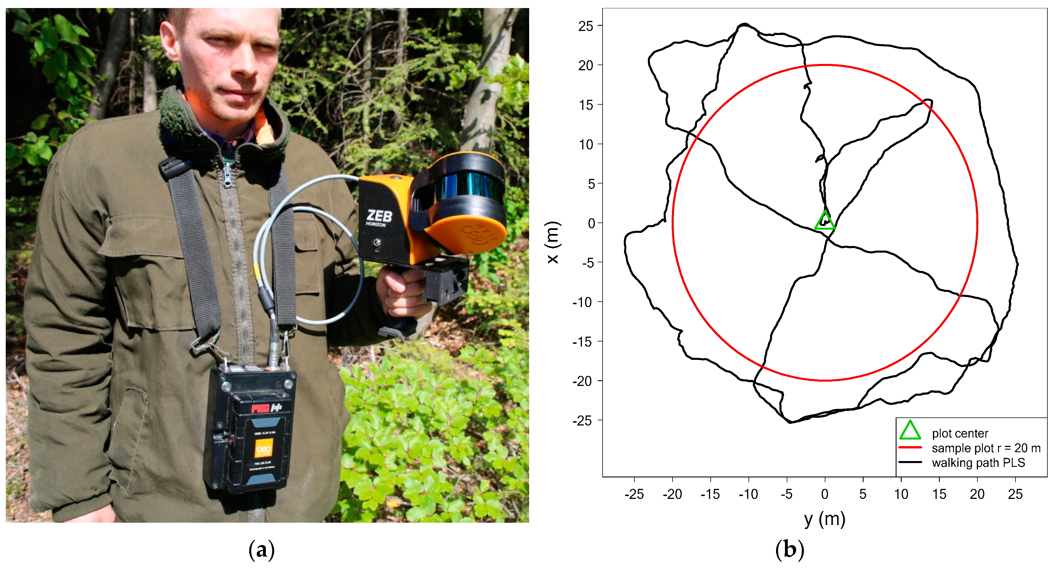
The 20 sample plots were scanned in March 2019 using a GeoSLAM ZEB HORIZON [26] (see Figure 1a) personal mobile laser scanner (PLS) (GeoSLAM Ltd., Nottingham, UK); for further technical information on the scanner, the reader is referred to Gollob et al. [28].
The data acquisition with ZEB HORIZON started with the initialization of the inertial measurement unit (IMU) to establish the coordinate reference system. For this purpose, the scanner was mounted on a tripod, which was positioned at the sample point. When the initialization was accomplished, usually after approximately 15 s, the scanner was demounted from the tripod, and was carried single-handedly along the walking path. During the scan process, the 3D measurement data were stored on the hard drive of the portable data logger in a highly compressed data format. After some initial trials, an optimum solution was determined for the walking path: The SLAM algorithm achieved both a relatively low scanner range noise and a low drift. By using this optimum walking path, the surveyor started at the sample point and moved northwards to the sample plot boundary. Afterward, the sample plot was completely circumvented once plus an extra quarter of the circumference. Then, the surveyor crossed the sample plot through the center to reach the opposite boundary. Subsequently, the surveyor walked along an additional quarter on the boundary, and moved afterward toward the center, where the scanner was finally fixed on the tripod again. A record of the walking path coordinates is shown in Figure 1b.
The entire walk, including the scan process and the data recording, consumed approximately 7–15 min. As a major advantage compared with the static terrestrial laser variant, the survey with the portable laser scanner does not require any target marks. These target marks are mandatory for a precise co-registration of multiple scans with a static TLS system; here, the spatial referencing of PLS data is performed on-the-fly using the SLAM algorithm.
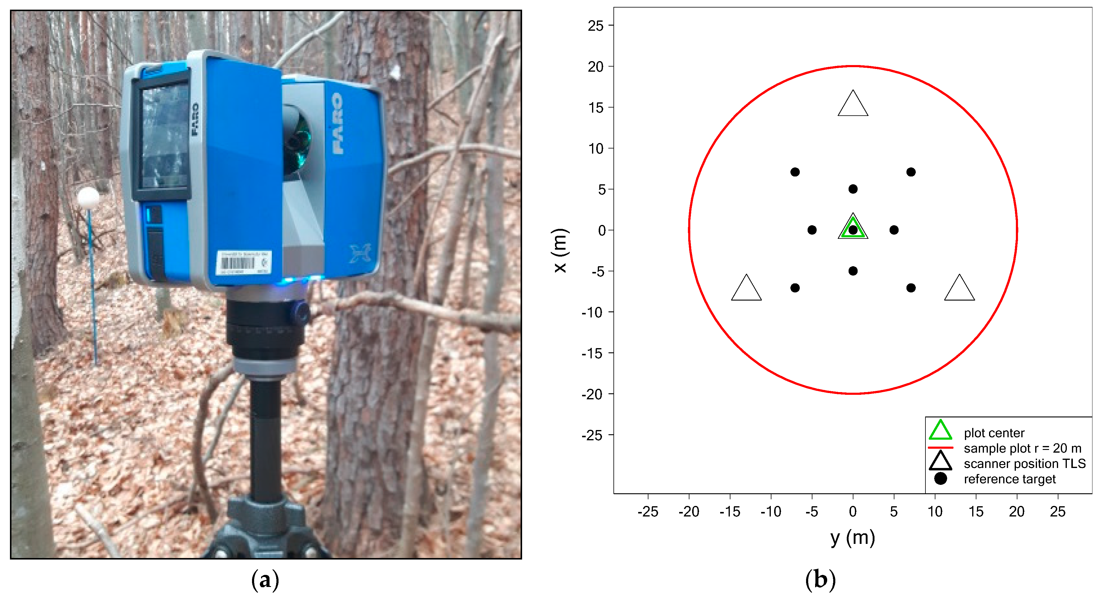
In February and March 2018, 17 out of the 20 sample plots surveyed with the PLS system were also scanned with the static FARO Focus3D X330 TLS system (Figure 2a) using MSA; for further information on the scanner and the hardware parameter settings, the reader is referred to Gollob et al. [6]. In our MSA setting, a single scan was conducted from the sample point position, and for three additional scans, the scanner was positioned at the corners of a triangle at a distance of 15 m from the center (Figure 2b). We found that this alignment provided the best compromise between labor cost and data quality. As the co-registration of the multiple scans required the extra positioning of target marks, nine Styrofoam spheres were placed on the sample plot. With static TLS and MSA, the total workload per sample plot was 49.6 min, out of which 32.6 min were consumed by the pure scan time plus photography, 12 min by the scanner installation, and 5 min by the installation of the target marks.
When data collection was accomplished with the portable laser scanner, the measurement data were transferred from the data logger onto a desktop computer using a USB flash drive. GeoSLAM Hub 5.2.0 software [39] was used for data pre-processing. The implemented SLAM algorithm performs the geo-tracking of the scanner in an unknown environment and the generation of the 3D point cloud raw data using both IMU data and feature detection algorithms. In so doing, the scanner position is registered using a moving time window across the raw data [21]. Since new data are added, the algorithm uses a linearized model to minimize the error of the IMU measurements together with the minimum search for the discrepancy between the 3D data points for each respective time segment [21]. For further details on the SLAM algorithm, the reader is referred to the manufacturer’s website: https://geoslam.com/slam/. According to the manufacturer, the accuracy of the measured points of the registered point cloud is 1–3 cm under normal sunlight conditions. The coordinates of the registered point cloud are represented by a local reference system with the start position of the walking path (sample point) being fixed at triple zero for the x, y, and z coordinates. The PLS data for each of the 20 sample plots were exported in LAS format, which is compatible with various point cloud software. For data export, the parameter settings “100% of points”, “time stamp: scan”, and “point color: none” were selected in GeoSLAM Hub 5.2.0.
The raw TLS scan data were co-registered with the FARO SCENE 6.2 program [40] and by using the coordinates of the Styrofoam spheres as reference points to merge the multiple scans into a single comprehensive point cloud. A constant cutoff distance of 30 m was chosen for each of the four scanner positions. The registered point cloud was represented by a local coordinate system using the first scan position (reference scan) at the plot center as zero references. The point cloud data were separately exported as CSV files for each of the 17 sample plots. The CSV TLS point clouds were then imported, transformed, and exported as LAS files using the functions fread() and write.las() in the R-packages data.table [41] and rlas [32].
The PLS and TLS point clouds were imported and clipped by an upright-oriented cylinder with a radius of 21 m and centered at the sample plot using the readLAS() function of the lidR package [31]. Hence, a 1-m-wide outer buffer was constructed around 20 radius plots. The lasground() function in the lidR package was then used to classify the data into ground points and vegetation points. The methodology of the classification implemented in lasground() uses a cloth simulation filter algorithm introduced by Zhang et al. [42]. Finally, the classified ground points were interpolated with the k-nearest neighbor method using grid_terrain() function implemented in the lidR package.
3.3. Accuracy of Tree Detection and dbh Measurement
In Gollob et al. [28], the quality of tree detection and dbh measurement was assessed in terms of three criteria: The detection rate , the commission error , and the overall accuracy :
where is the number of correctly found reference trees, is the total number of reference trees, is the number of tree positions that could not be assigned to an existing tree in the reference data, is the number of automatically detected tree positions (), and is the omission error, defined as . The detection rate measures the proportion of the correctly detected tree locations, the commission error evaluates the proportion of falsely detected tree locations, and the overall accuracy is a combination of the latter two metrics and represents a global quality criterion.
The precision of the automatic dbh measurements was assessed by means of root-mean-square error (RMSE) calculated as the square root of the average quadratic distance between the automatic measurement and the corresponding reference measurement :
The accuracy of the automatic dbh measurements was assessed in terms of bias:
The latter two criteria were also calculated as relative measures, that is, as percentage RMSE (RMSE%) and percentage bias (bias%):
with
being the average dbh of the reference data.
To guarantee meaningful comparisons with the results presented in Gollob et al. [28], future users of this dataset are likewise encouraged to evaluate their results using these performance measures. In this dataset, we provide the above-described performance measures on two different aggregation levels. Thus, besides the overall performance measures evaluated across the complete sample, these measures are also separately reported per sample plot (Section 2.4.).
4. User Notes
The chosen data repository supports versioning of datasets; this data descriptor refers to version 1.0. The dataset will be updated in the future when new 3D data and reference measurements are collected on this or other sample plots. Users can find updated and original versions of the dataset under the same doi:10.5281/zenodo.3698956 [25].
5. Discussion
Providing datasets is regarded as essential for benchmarking and comparative performance tests of the different algorithms, especially in the field of forest inventory, where novel measurement technology for LiDAR-based sensors is currently being introduced. Only if the same data basis and the same criteria are used, it is possible to reveal the true potential of PLS compared with TLS in particular. Beyond the approaches for tree detection and dbh measurement that were presented in Gollob et al. [28], the dataset also offers the possibility of automatically estimating tree heights and crown bases from PLS and TLS data, and it also enables the comparison of the achieved results with the provided reference data. Besides creating new DTMs, other developers can alternatively access the DTMs provided with this dataset. This will probably help to avoid possible confounding effects that may occur when different routines are used for vegetation/ground classification or for the spatial interpolations of DTM grids. However, a direct comparison of the DTMs from both sensors (static TLS and portable PLS) is not possible because the DTMs derived from both sensors differ in an offset, which varies per plot. It should be noted that the created DTMs were only valid locally. If DTMs were required for larger areas, it would be beneficial to use ALS data. In addition to the abovementioned possible use cases of the dataset, it is also worth noting that, to the best of our knowledge, it is the first publicly available dataset of the GeoSLAM ZEB HORIZON in a forest inventory context. This enables the reader to assess the data quality provided by the novel device.
Regarding the reference dataset, it is worth noting that these field measurements were recorded with pencils on paper and thereafter manually transcribed into an electronic database. Thus, the existence of possible entry errors cannot be excluded. Other possible errors in the manual measurements may result from imprecise height, diameter, and position measuring, or tilted trees. For the comparison of algorithms, however, this is only a minor problem, since all algorithms are evaluated against the same reference data. Regarding the point cloud quality, it is worth noting that in the presented dataset, instrumental drift and registration inaccuracies were neither a problem for PLS nor TLS.
Initial tests on large experimental stands showed that for PLS, longer recording times (greater than 30 min) yielded instrumental drift and registration problems, while for TLS, an increasing number of scans complicates co-registration and adds additional noise. However, a list of tree positions and dimensions could be created more completely and efficiently with PLS. With TLS, the tree dimensions (especially the diameters) were more precise.
Author Contributions
Conceptualization, C.G., T.R., and A.N.; data curation, C.G. and T.R.; investigation, C.G. and T.R.; formal analysis, C.G., T.R., and A.N.; methodology, C.G., T.R., and A.N.; software, C.G., T.R., and A.N.; supervision, A.N.; validation, G.G. and T.R.; writing—original draft, C.G., T.R., and A.N.; writing—review and editing, C.G., T.R., and A.N. All authors have read and agreed to the published version of the manuscript.
Funding
The open access publishing was supported by BOKU Vienna Open Access Publishing Fund.
Acknowledgments
The authors appreciate the careful point cloud measurement and support during the fieldwork provided by Stefan Ebner, Tobias Ofner, Valentin Sarkleti, Stefan Stulik, Philip Svazek and Clemens Wassermann. The authors would like to thank the anonymous reviewers for their thoughtful comments and suggestions on the original manuscript.
Conflicts of Interest
The authors declare no conflict of interest.
References
- Kershaw, J.A.; Ducey, M.J.; Beers, T.W.; Husch, B. Forest Mensuration; John Wiley & Sons, Ltd.: Chichester, UK, 2016; ISBN 9781118902028. [Google Scholar]
- Köhl, M.; Magnussen, S.; Marchetti, M. Sampling Methods, Remote Sensing and GIS Multiresource Forest Inventory; Tropical Forestry; Springer: Berlin/Heidelberg, Germany, 2006; ISBN 978-3-540-32571-0. [Google Scholar]
- Kauffman, J.B.; Arifanti, V.B.; Basuki, I.; Kurnianto, S.; Novita, N.; Murdiyarso, D.; Donato, D.C.; Warren, M.W. Protocols for the Measurement, Monitoring, and Reporting of Structure, Biomass, Carbon Stocks and Greenhouse Gas Emissions in Tropical Peat Swamp Forests; Center for International Forestry Research (CIFOR): Bogor, Indonesia, 2017. [Google Scholar]
- Kramer, H.; Akça, A. Leitfaden zur Waldmesslehre, 5th ed.; Sauerländer, J D: Frankfurt/Main, Germany, 2008; ISBN 3793908305. [Google Scholar]
- Liang, X.; Hyyppä, J.; Kaartinen, H.; Lehtomäki, M.; Pyörälä, J.; Pfeifer, N.; Holopainen, M.; Brolly, G.; Francesco, P.; Hackenberg, J.; et al. International benchmarking of terrestrial laser scanning approaches for forest inventories. ISPRS J. Photogramm. Remote Sens. 2018, 144, 137–179. [Google Scholar] [CrossRef]
- Gollob, C.; Ritter, T.; Wassermann, C.; Nothdurft, A. Influence of Scanner Position and Plot Size on the Accuracy of Tree Detection and Diameter Estimation Using Terrestrial Laser Scanning on Forest Inventory Plots. Remote Sens. 2019, 11, 1602. [Google Scholar] [CrossRef] [Green Version]
- Ritter, T.; Nothdurft, A. Automatic assessment of crown projection area on single trees and stand-level, based on three-dimensional point clouds derived from terrestrial laser-scanning. Forests 2018, 9, 237. [Google Scholar] [CrossRef] [Green Version]
- Ritter, T.; Schwarz, M.; Tockner, A.; Leisch, F.; Nothdurft, A. Automatic mapping of forest stands based on three-dimensional point clouds derived from terrestrial laser-scanning. Forests 2017, 8, 265. [Google Scholar] [CrossRef]
- Liang, X.; Kankare, V.; Hyyppä, J.; Wang, Y.; Kukko, A.; Haggrén, H.; Yu, X.; Kaartinen, H.; Jaakkola, A.; Guan, F.; et al. Terrestrial laser scanning in forest inventories. ISPRS J. Photogramm. Remote Sens. 2016, 115, 63–77. [Google Scholar] [CrossRef]
- Tang, J.; Chen, Y.; Chen, L.; Liu, J.; Hyyppä, J.; Kukko, A.; Kaartinen, H.; Hyyppä, H.; Chen, R.; Khoshelham, K.; et al. Fast Fingerprint Database Maintenance for Indoor Positioning Based on UGV SLAM. Sensors 2015, 15, 5311–5330. [Google Scholar] [CrossRef] [Green Version]
- Pueschel, P.; Newnham, G.; Rock, G.; Udelhoven, T.; Werner, W.; Hill, J. The influence of scan mode and circle fitting on tree stem detection, stem diameter and volume extraction from terrestrial laser scans. ISPRS J. Photogramm. Remote Sens. 2013, 77, 44–56. [Google Scholar] [CrossRef]
- Maltamo, M.; Næsset, E.; Vauhkonen, J. Forestry Applications of Airborne Laser Scanning: Concepts and Case Studies. Manag. Ecosyst. 2014, 27, 3–41. [Google Scholar]
- Lindberg, E.; Hollaus, M. Comparison of methods for estimation of stem volume, stem number and basal area from airborne laser scanning data in a hemi-boreal forest. Remote Sens. 2012, 4, 1004–1023. [Google Scholar] [CrossRef] [Green Version]
- Korhonen, L.; Vauhkonen, J.; Virolainen, A.; Hovi, A.; Korpela, I. Estimation of tree crown volume from airborne lidar data using computational geometry. Int. J. Remote Sens. 2013, 34, 7236–7248. [Google Scholar] [CrossRef]
- Vauhkonen, J.; Næsset, E.; Gobakken, T. Deriving airborne laser scanning based computational canopy volume for forest biomass and allometry studies. ISPRS J. Photogramm. Remote Sens. 2014, 96, 57–66. [Google Scholar] [CrossRef]
- Yu, X.; Hyyppä, J.; Kaartinen, H.; Maltamo, M. Automatic detection of harvested trees and determination of forest growth using airborne laser scanning. Remote Sens. Environ. 2004, 90, 451–462. [Google Scholar] [CrossRef]
- Liang, X.; Kukko, A.; Kaartinen, H.; Hyyppä, J.; Yu, X.; Jaakkola, A.; Wang, Y. Possibilities of a Personal Laser Scanning System for Forest Mapping and Ecosystem Services. Sensors 2014, 14, 1228–1248. [Google Scholar] [CrossRef] [PubMed]
- Maltamo, M.; Bollandsas, O.M.; Naesset, E.; Gobakken, T.; Packalen, P. Different plot selection strategies for field training data in ALS-assisted forest inventory. Forestry 2011, 84, 23–31. [Google Scholar] [CrossRef] [Green Version]
- Holopainen, M.; Kankare, V.; Vastaranta, M.; Liang, X.; Lin, Y.; Vaaja, M.; Yu, X.; Hyyppä, J.; Hyyppä, H.; Kaartinen, H.; et al. Tree mapping using airborne, terrestrial and mobile laser scanning – A case study in a heterogeneous urban forest. Urban For. Urban Green. 2013, 12, 546–553. [Google Scholar] [CrossRef]
- Liang, X.; Hyyppä, J.; Kukko, A.; Kaartinen, H.; Jaakkola, A.; Yu, X. The Use of a Mobile Laser Scanning System for Mapping Large Forest Plots. IEEE Geosci. Remote Sens. Lett. 2014, 11, 1504–1508. [Google Scholar] [CrossRef]
- Ryding, J.; Williams, E.; Smith, M.; Eichhorn, M. Assessing Handheld Mobile Laser Scanners for Forest Surveys. Remote Sens. 2015, 7, 1095–1111. [Google Scholar] [CrossRef] [Green Version]
- Chen, S.; Liu, H.; Feng, Z.; Shen, C.; Chen, P. Applicability of personal laser scanning in forestry inventory. PLoS ONE 2019, 14, e0211392. [Google Scholar] [CrossRef]
- Liang, X.; Kukko, A.; Hyyppä, J.; Lehtomäki, M.; Pyörälä, J.; Yu, X.; Kaartinen, H.; Jaakkola, A.; Wang, Y. In-situ measurements from mobile platforms: An emerging approach to address the old challenges associated with forest inventories. ISPRS J. Photogramm. Remote Sens. 2018, 143, 97–107. [Google Scholar] [CrossRef]
- Bauwens, S.; Bartholomeus, H.; Calders, K.; Lejeune, P. Forest Inventory with Terrestrial LiDAR: A Comparison of Static and Hand-Held Mobile Laser Scanning. Forests 2016, 7, 127. [Google Scholar] [CrossRef] [Green Version]
- Gollob, C.; Ritter, T.; Nothdurft, A. LAUT - Terrestrial and Personal laser scanner data from Austrian forest Inventory plots. Zenodo 2020. [Google Scholar] [CrossRef]
- ZEB Horizon - GeoSLAM. Available online: https://geoslam.com/solutions/zeb-horizon/ (accessed on 13 January 2020).
- FARO Laser Scanner Focus3D X 330 Features, Benefits & Technical Specifications. Available online: https://faro.app.box.com/s/8ilpeyxcuitnczqgsrgp5rx4a9lb3skq/file/441668110322 (accessed on 29 April 2020).
- Gollob, C.; Ritter, T.; Nothdurft, A. Forest Inventory with Long Range and High-Speed Personal Laser Scanning (PLS) and Simultaneous Localization and Mapping (SLAM) Technology. Remote Sens. 2020, 12, 1509. [Google Scholar] [CrossRef]
- Girardeau-Montaut, D.C. 3D Point Cloud and Mesh Processing Software; Telecom ParisTechs: Palaiseau, France, 2017. [Google Scholar]
- R Core Team. R: A Language and Environment for Statistical Computing, R Version 3.5.1; R Foundation for Statistical Computing: Vienna, Austria, 2018. [Google Scholar]
- Roussel, J.-R.; Auty, D.; Romain, J.-R.; Auty, D.; De Boissieu, F.; Meador Sánchez, A. lidR: Airborne LiDAR Data Manipulation and Visualization for Forestry Applications 2019; R Foundation for Statistical Computing: Vienna, Austria, 2019. [Google Scholar]
- Roussel, J.-R.; De Boissieu, F. rlas: Read and Write “las” and “laz” Binary File Formats Used for Remote Sensing Data 2019; R Foundation for Statistical Computing: Vienna, Austria, 2019. [Google Scholar]
- Müller, C.H.; Garlipp, T. Simple consistent cluster methods based on redescending M-estimators with an application to edge identification in images. J. Multivar. Anal. 2005, 92, 359–385. [Google Scholar] [CrossRef] [Green Version]
- Chernov, N. Circular and Linear Regression: Fitting Circles and Lines by Least Squares; Taylor & Francis: Boca Raton, FL, USA, 2011; ISBN 9781439835906. [Google Scholar]
- Fitzgibbon, A.W.; Pilu, M.; Fisher, R.B. Direct least squares fitting of ellipses. In Proceedings of the International Conference on Pattern Recognition, Vienna, Austria, 25–29 August 1996; Institute of Electrical and Electronics Engineers Inc.: New York, NY, USA, 1996; Volume 1, pp. 253–257. [Google Scholar]
- Bitterlich, W. Die Winkelzählprobe. Allg. forst- und holzwirtschaftliche Zeitung 1948, 59, 4–5. [Google Scholar] [CrossRef]
- Bitterlich, W. Die Winkelzählprobe. Forstwissenschaftliches Cent. 1952, 71, 215–225. [Google Scholar] [CrossRef]
- Bitterlich, W. The Relascope Idea. Relative Measurements in Forestry; Commonwealth Agricultural Bureau: Oxfordshire, UK, 1984; ISBN 0851985394. [Google Scholar]
- Hub—GeoSLAM. Available online: https://geoslam.com/solutions/geoslam-hub/ (accessed on 13 January 2020).
- FARO SCENE FARO Technologies. Available online: https://www.faro.com/products/construction-bim-cim/faro-scene/ (accessed on 23 February 2019).
- Dowle, M.; Srinivasan, A.; Gorecki, J.; Chirico, M.; Stetsenko, P.; Short, T.; Lianoglou, S.; Antonyan, E.; Bonsch, M.; Parsonage, H.; et al. Data.Table: Extension of “Data.Frame”, version 1.12.8; CRAN, 2019. Available online: https://cran.r-project.org/package=data.table (accessed on 30 June 2020).
- Zhang, W.; Qi, J.; Wan, P.; Wang, H.; Xie, D.; Wang, X.; Yan, G. An Easy-to-Use Airborne LiDAR Data Filtering Method Based on Cloth Simulation. Remote Sens. 2016, 8, 501. [Google Scholar] [CrossRef]
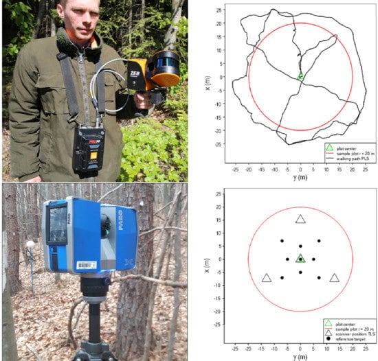
Figure 1.
(a) ZEB HORIZON PLS in operation. (b) Walking path for the PLS data acquisitions (starting and ending in plot center) and sample plot.
Figure 1.
(a) ZEB HORIZON PLS in operation. (b) Walking path for the PLS data acquisitions (starting and ending in plot center) and sample plot.

Figure 2.
(a) FARO Focus3D X330. (b) TLS scan setting with reference targets.


Table 1.
A number of 3D points and scanning time for personal laser scanner (PLS) and terrestrial laser scanner (TLS) point cloud data.
Table 1.
A number of 3D points and scanning time for personal laser scanner (PLS) and terrestrial laser scanner (TLS) point cloud data.
| Plot_Id | PLS | TLS | ||
|---|---|---|---|---|
| No. of 3D Points | Scan Time (Min) | No. of 3D Points | Scan Time (Min) | |
| 1 | 56,611,058 | 9.1 | 54,200,866 | 32.6 |
| 2 | 39,561,515 | 7.3 | NA | NA |
| 3 | 65,376,686 | 11.7 | 51,758,722 | 32.6 |
| 4 | 84,874,023 | 12.0 | 54,241,249 | 32.6 |
| 5 | 84,776,235 | 13.4 | 60,538,323 | 32.6 |
| 6 | 61,947,561 | 10.7 | 56,786,129 | 32.6 |
| 7 | 68,107,655 | 13.9 | 48,311,934 | 32.6 |
| 8 | 89,301,650 | 13.5 | 50,517,017 | 32.6 |
| 9 | 87,808,373 | 15.5 | 73,871,487 | 32.6 |
| 10 | 44,758,685 | 8.5 | 67,626,474 | 32.6 |
| 11 | 68,386,176 | 11.4 | 52,367,494 | 32.6 |
| 12 | 48,101,125 | 10.6 | 55,318,186 | 32.6 |
| 13 | 76,584,233 | 13.1 | 60,120,291 | 32.6 |
| 14 | 32,588,141 | 8.6 | 59,840,384 | 32.6 |
| 15 | 65,827,042 | 10.6 | 61,178,842 | 32.6 |
| 16 | 66,709,730 | 12.1 | 61,928,447 | 32.6 |
| 17 | 57,766,481 | 9.8 | 57,557,937 | 32.6 |
| 18 | 61,846,976 | 11.0 | 61,994,593 | 32.6 |
| 19 | 36,971,082 | 8.0 | NA | NA |
| 20 | 45,658,647 | 8.3 | NA | NA |
Table 2.
Dataset fields describing PLS and TLS point clouds. ALS, Airborne laser scanning.
| Header | Description | Unit |
|---|---|---|
| X | X coordinate in local coordinate reference system | m |
| Y | Y coordinate in local coordinate reference system | m |
| Z | Z coordinate in local coordinate reference system | m |
| gpstime | Time at which the point was recorded; always 0 for TLS; starts from 0 for PLS | s |
| Intensity | Intensity of the returned pulse; always 0 for TLS | - |
| ReturnNumber | Pulse return number for a given output pulse; created for ALS, not meaningful for PLS/TLS; always 0 | - |
| NumberOfReturns | Total number of returns for a given pulse; created for ALS, not meaningful for PLS/TLS | - |
| ScanDirectionFlag | Direction at which the scanner mirror was traveling at the time of the output pulse; created for ALS, not meaningful for PLS/TLS; always 0 | - |
| EdgeOfFlightline | A value of 1 only when the point is at the end of a scan; created for ALS, not meaningful for PLS/TLS; always 0 | - |
| Classification | 1: Vegetation point; 2: Ground point | - |
| Synthetic_flag | If set, this point was created by a technique other than LiDAR collection; always FALSE | - |
| Keypoint_flag | If set, this point is considered to be a model key-point; always FALSE | - |
| Withheld_flag | If set, this point should not be included in processing; always FALSE | - |
| ScanAngleRank | The angle at which the laser point was output from the laser system, including the roll of the aircraft; created for ALS, not meaningful for PLS/TLS; always 0 | degrees |
| UserData | Can be used at the user’s discretion; always 0 | - |
| PointSourceID | Value of 0 implies that this point originated in this file; always 0 | - |
Table 3.
Summary statistics of digital terrain models (DTMs).
| # of sample plots | 20 | ||||
| pixel resolution | 20 × 20 cm | ||||
| Mean | SD | Min | Max | ||
| PLS | minimum height (m) | −7.7 | 2.0 | −12.0 | −3.9 |
| maximum height (m) | 5.0 | 2.4 | 0.3 | 8.7 | |
| mean height (m) | −1.1 | 0.5 | −1.9 | 0.1 | |
| height difference (m) | 12.7 | 4.1 | 4.2 | 20.5 | |
| SD height (m) | 3.2 | 1.1 | 0.8 | 5.3 | |
| TLS | minimum height (m) | −6.1 | 2.1 | −10.6 | −2.4 |
| maximum height (m) | 5.6 | 2.3 | 1.7 | 9.2 | |
| mean height (m) | 0.0 | 0.5 | −1.0 | 1.2 | |
| height difference (m) | 11.7 | 4.2 | 4.1 | 19.5 | |
| SD height (m) | 3.0 | 1.1 | 0.8 | 5.1 | |
Note: Minimum height, minimum pixel value per sample plot; maximum height, maximum pixel value per sample plot; mean height, average pixel value per sample plot; height difference, maximum difference in pixel values per sample plot; SD height, standard deviation of pixel values per sample plot.
Table 4.
Summary statistics of reference measurements on sample plots.
| # of sample plots | 20 | |||
| # of trees | 2524 | |||
| # of trees/sample plot | 126.2 | |||
| Mean | SD | Min | Max | |
| slope (%) | 29.4 | 10.2 | 10.5 | 51.0 |
| dbh (cm) | 18.7 | 13.0 | 5.0 | 74.0 |
| h (m) | 21.9 | 9.9 | 4.0 | 44.4 |
| cb (m) | 11.4 | 7.2 | 0.0 | 29.9 |
Note: Slope, terrain slope of sample plot; dbh, diameter at breast height; h, tree height; cb, height of crown base.
Table 5.
Dataset fields describing reference data and automatic tree detection and dbh estimation results.
Table 5.
Dataset fields describing reference data and automatic tree detection and dbh estimation results.
| Header | Description | Unit |
|---|---|---|
| plot_id | Sample plot ID | - |
| slope | Terrain slope of sample plot | m |
| tree_id | Z coordinate | m |
| X | X coordinate of the tree | m |
| Y | Y coordinate of the tree | m |
| tree_spec | Tree species: be, beech (Fagus silvatica); sp, spruce (Picea abies); fir, fir (Abies alba); la, larch (Larix decidua); oak, oak (Quercus petraea, Q. robur); pin, pine (Pinus silvestris, P. nigra, P. strobus); pop, poplar (Populus nigra, P. x hybrida); sall; sallow (Salix spec.); bir, birch (Betula pendula, B. pubescens); hb, hornbeam (Caprinus betulus); cher, cherry (Prunus avium); map; maple (Acer pseudoplatanus, A. platanoides, A. campestre); elm, elm (Ulmus glabra, U. minor); ash, ash (Fraxinus excelsior) | - |
| dbh | Diameter at breast height (1.3 m above ground) | cm |
| h | Tree height | m |
| cb | Height of crown base | m |
| scanner | Used scanner device: PLS/TLS, PLS, TLS | - |
| detection_PLS | Tree was detected: correct, non, false; using the algorithm of Gollob et al. [28] | - |
| detection_TLS | Tree was detected: correct, non, false; using the algorithm of Gollob et al. [28] | - |
| d_circ_PLS | Estimated dbh with circle fit to the PLS data, using the circular cluster method of Müller and Garlipp [33] | cm |
| d_circ_TLS | Estimated dbh with circle fit to the TLS data, using the circular cluster method of Müller and Garlipp [33] | cm |
| d_circ2_PLS | Estimated dbh with circle fit to the PLS data, using the least-squares-based algorithm of Chernov [34] | cm |
| d_circ2_TLS | Estimated dbh with circle fit to the TLS data, using the least-squares-based algorithm of Chernov [34] | cm |
| d_ell_PLS | Estimated dbh with ellipse fit to the PLS data, using the least-squares-based algorithm of Fitzgibbon et al. [35] | cm |
| d_ell_TLS | Estimated dbh with ellipse fit to the TLS data, using the least-squares-based algorithm of Fitzgibbon et al. [35] | cm |
| d_gam_PLS | Estimated dbh with spline fit to the PLS data, using the algorithm of Gollob et al. [28] | cm |
| d_gam_TLS | Estimated dbh with spline fit to the TLS data, using the algorithm of Gollob et al. [28] | cm |
| d_tegam_PLS | Estimated dbh with tensor spline fit to the PLS data, using the algorithm of Gollob et al. [28] | cm |
| d_tegam_TLS | Estimated dbh with tensor spline fit to the TLS data, using the algorithm of Gollob et al. [28] | cm |
Table 6.
Dataset fields describing the evaluation of automatic tree detection and dbh estimation.
| Header | Description | Unit |
|---|---|---|
| plot_id | Sample plot ID | - |
| scanner | Used scanner device: PLS (ZEB Horizon, GeoSLAM Ltd., Nottingham, UK [26]), TLS (Focus3D X330, Faro Technologies Inc., Lake Mary, FL, USA [27]) | - |
| dr | Detection rate | % |
| c | Commission rate | % |
| acc | Overall accuracy | % |
| RMSE_d_circ | RMSE of dbh estimated by circle fit using the circular cluster method of Müller and Garlipp [33] | cm |
| RMSE_d_circ2 | RMSE of dbh estimated by circle fit using the least-squares-based algorithm of Chernov [34] | cm |
| RMSE_d_ell | RMSE of dbh estimated by ellipse fit using the least-squares-based algorithm of Fitzgibbon et al. [35] | cm |
| RMSE_d_gam | RMSE of dbh estimated by spline fit using the algorithm of Gollob et al. [28] | cm |
| RMSE_d_tegam | RMSE of dbh estimated by tensor spline fit using the algorithm of Gollob et al. [28] | cm |
| RMSErel_d_circ | Relative RMSE of dbh estimated by circle fit using the circular cluster method of Müller and Garlipp [33] | % |
| RMSErel_d_circ2 | Relative RMSE of dbh estimated by circle fit using the least-squares-based algorithm of Chernov [34] | % |
| RMSErel_d_ell | Relative RMSE of dbh estimated by ellipse fit using the least-squares-based algorithm of Fitzgibbon et al. [35] | % |
| RMSErel_d_gam | Relative RMSE of dbh estimated by spline fit using the algorithm of Gollob et al. [28] | % |
| RMSErel_d_tegam | Relative RMSE of dbh estimated by tensor spline fit using the algorithm of Gollob et al. [28] | % |
| bias_d_circ | Bias of dbh estimated by circle fit using the circular cluster method of Müller and Garlipp [33] | cm |
| bias_d_circ2 | Bias of dbh estimated by circle fit using the least-squares-based algorithm of Chernov [34] | cm |
| bias_d_ell | Bias of dbh estimated by ellipse fit using the least-squares-based algorithm of Fitzgibbon et al. [35] | cm |
| bias_d_gam | Bias of dbh estimated by spline fit using the algorithm of Gollob et al. [28] | cm |
| bias_d_tegam | Bias of dbh estimated by tensor spline fit using the algorithm of Gollob et al. [28] | cm |
| biasrel_d_circ | Relative bias of dbh estimated by circle fit using the circular cluster method of Müller and Garlipp [33] | % |
| biasrel_d_circ2 | Relative bias of dbh estimated by circle fit using the least-squares-based algorithm of Chernov [34] | % |
| biasrel_d_ell | Relative bias of dbh estimated by ellipse fit using the least-squares-based algorithm of Fitzgibbon et al. [35] | % |
| biasrel_d_gam | Relative bias of dbh estimated by spline fit using the algorithm of Gollob et al. [28] | % |
| biasrel_d_tegam | Relative bias of dbh estimated by tensor spline fit using the algorithm of Gollob et al. [28] | % |
Publisher’s Note: MDPI stays neutral with regard to jurisdictional claims in published maps and institutional affiliations. |
© 2020 by the authors. Licensee MDPI, Basel, Switzerland. This article is an open access article distributed under the terms and conditions of the Creative Commons Attribution (CC BY) license (http://creativecommons.org/licenses/by/4.0/).
Share and Cite
MDPI and ACS Style
Gollob, C.; Ritter, T.; Nothdurft, A. Comparison of 3D Point Clouds Obtained by Terrestrial Laser Scanning and Personal Laser Scanning on Forest Inventory Sample Plots. Data 2020, 5, 103. https://0-doi-org.brum.beds.ac.uk/10.3390/data5040103
AMA Style
Gollob C, Ritter T, Nothdurft A. Comparison of 3D Point Clouds Obtained by Terrestrial Laser Scanning and Personal Laser Scanning on Forest Inventory Sample Plots. Data. 2020; 5(4):103. https://0-doi-org.brum.beds.ac.uk/10.3390/data5040103
Chicago/Turabian StyleGollob, Christoph, Tim Ritter, and Arne Nothdurft. 2020. "Comparison of 3D Point Clouds Obtained by Terrestrial Laser Scanning and Personal Laser Scanning on Forest Inventory Sample Plots" Data 5, no. 4: 103. https://0-doi-org.brum.beds.ac.uk/10.3390/data5040103