First 1-M Resolution Land Cover Map Labeling the Overlap in the 3rd Dimension: The 2018 Map for Wallonia


 , , ,
, , ,
Abstract
:1. Summary
2. Data Description
2.1. Data Format
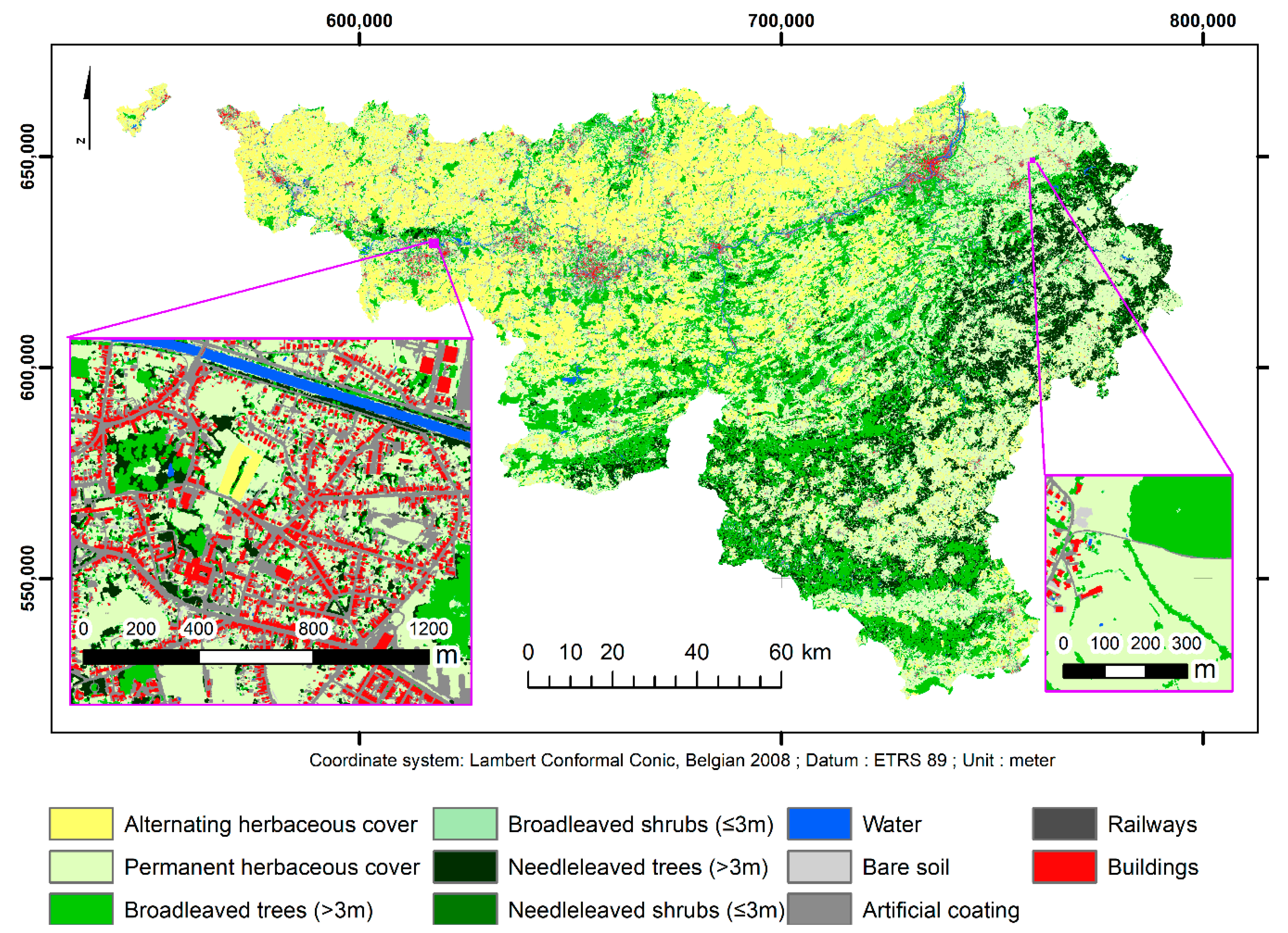
2.2. Land Cover Legend
2.3. Strengths of the LC Map
2.4. Accuracy Assessment
3. Methods
3.1. Data Design
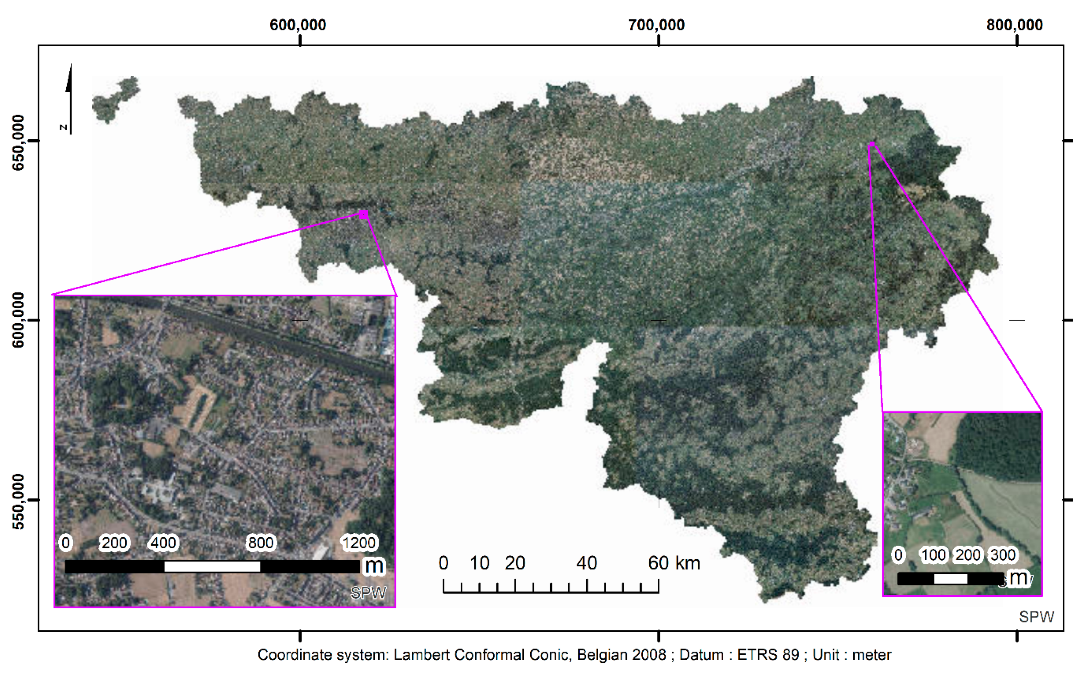
3.2. Input Data
3.3. Image Classification
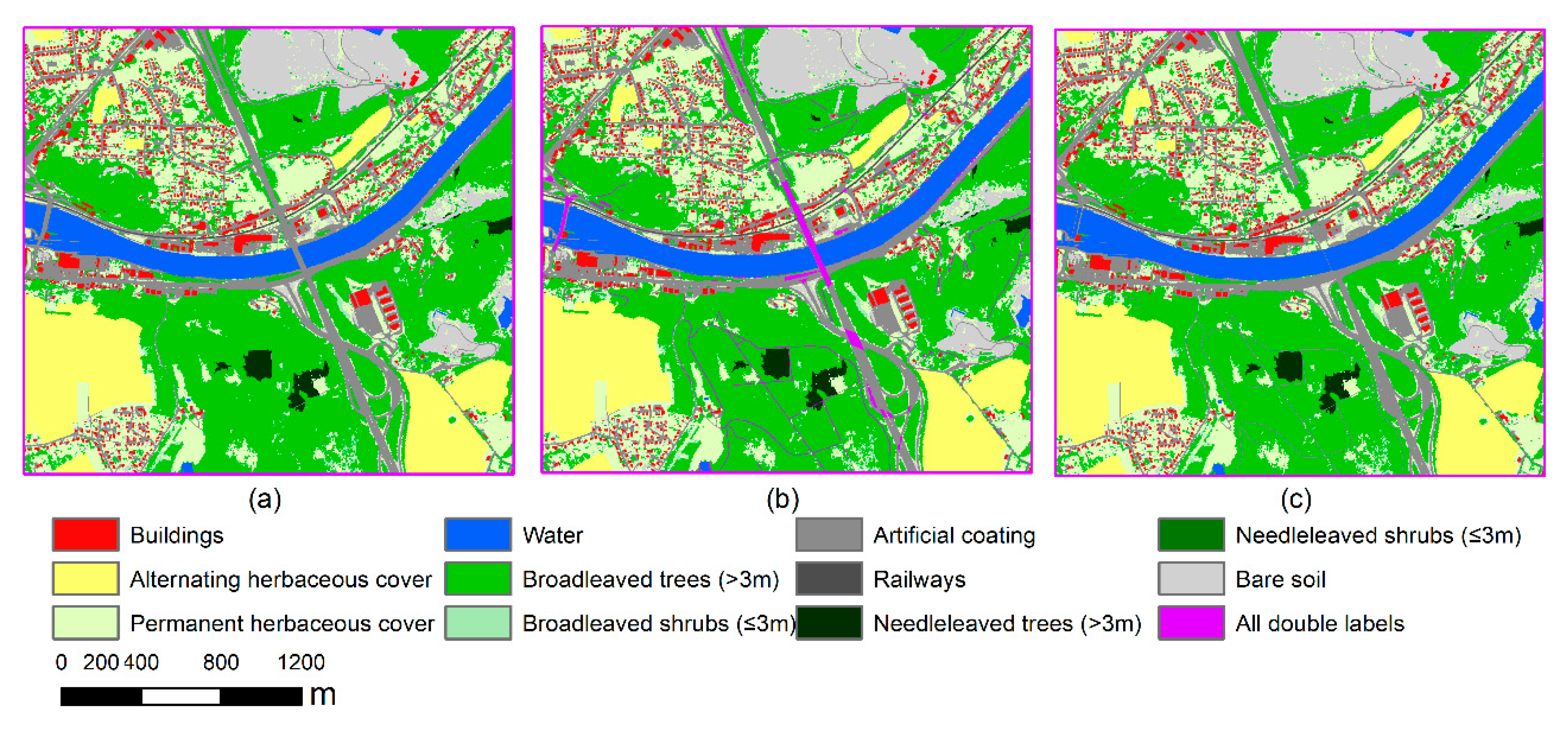
3.4. Data Fusion
3.5. Post-Processing
4. User Notes
Author Contributions
Funding
Acknowledgments
Conflicts of Interest
References
- Beaumont, B.; Stephenne, N.; Wyard, C.; Hallot, E. Users’ consultation process in building a land cover and land use database for the official Walloon Georeferential. In Proceedings of the 2019 Joint Urban, Remote Sensing Event (JURSE), Vannes, France, 22–24 May 2019; pp. 1–4. [Google Scholar]
- Beaumont, B.; Grippa, T.; Lennert, M. A user-driven process for INSPIRE compliant Land Use database: Example from Wallonia, Belgium. Ann. GIS 2021, accepted. [Google Scholar]
- Bourdouxhe, A.; Duflot, R.; Radoux, J.; Dufrêne, M. Comparison of methods to model species habitat networks for decision-making in nature conservation: The case of the wildcat in southern Belgium. J. Nat. Conserv. 2020, 58, 125901. [Google Scholar] [CrossRef]
- Olofsson, P.; Foody, G.; Herold, M.; Stehman, S.; Woodcock, C.; Wulder, M. Good Practices for Assessing Accuracy and Estimating Area of Land Change. Remote Sens. Environ. 2013, 148, 42–57. [Google Scholar] [CrossRef]
- Stehman, S.V. Estimating area from an accuracy assessment error matrix. Remote Sens. Environ. 2013, 132, 202–211. [Google Scholar] [CrossRef]
- INSPIRE Thematic Working Group Land Cover. INSPIRE Data Specification for the Spatial Data Theme Land Cover; D2.8.II.2_v3.0rc3, 4.2.2013; INSPIRE Thematic Working Group: London, UK, 2013. [Google Scholar]
- Radoux, J.; Bourdouxhe, A.; Coos, W.; Dufrêne, M.; Defourny, P. Improving ecotope segmentation by combining topographic and spectral data. Remote Sens. 2019, 11, 354. [Google Scholar] [CrossRef] [Green Version]
- Lennert, M.; Grippa, T.; Radoux, J.; Bassine, C.; Beaumont, B.; Defourny, P.; Wolff, E. Creating wallonia’s new very high resolution land cover maps: Combining grass gis obia and otb pixel-based results. Int. Arch. Photogramm. Remote Sens. Spat. Inf. Sci. 2019, XLII-4/W14, 151–157. [Google Scholar] [CrossRef] [Green Version]
- Grizonnet, M.; Michel, J.; Poughon, V.; Inglada, J.; Savinaud, M.; Cresson, R. Orfeo ToolBox: Open source processing of remote sensing images. Open Geospat. Data Softw. Stand. 2017, 2, 1–8. [Google Scholar] [CrossRef] [Green Version]
- Radoux, J.; Lamarche, C.; Van Bogaert, E.; Bontemps, S.; Brockmann, C.; Defourny, P. Automated training sample extraction for global land cover mapping. Remote Sens. 2014, 6, 3965–3987. [Google Scholar] [CrossRef] [Green Version]
- Comaniciu, D.; Meer, P. Mean shift: A robust approach toward feature space analysis. IEEE Trans. Pattern Anal. Mach. Intell. 2002, 24, 603–619. [Google Scholar] [CrossRef] [Green Version]
- Ng, V.; Hofmann, D. Scalable Feature Extraction with aerial and Satellite Imagery. In Proceedings of the 17th Python in Science Conference (SCIPY 2018), Austin, TX, USA, 9–15 July 2018; pp. 145–151. [Google Scholar]
- Neteler, M.; Bowman, M.H.; Landa, M.; Metz, M. GRASS GIS: A multi-purpose open source GIS. Environ. Model. Softw. 2012, 31, 124–130. [Google Scholar] [CrossRef] [Green Version]
- Grippa, T.; Lennert, M.; Beaumont, B.; Vanhuysse, S.; Stephenne, N.; Wolff, E. An open-source semi-automated processing chain for urban object-based classification. Remote Sens. 2017, 9, 358. [Google Scholar] [CrossRef] [Green Version]
- Beaumont, B.; Grippa, T.; Lennert, M.; Vanhuysse, S.G.; Stephenne, N.R.; Wolff, E. Toward an operational framework for fine-scale urban land-cover mapping in Wallonia using submeter remote sensing and ancillary vector data. J. Appl. Remote Sens. 2017, 11, 036011. [Google Scholar] [CrossRef] [Green Version]
- Grippa, T.; Georganos, S.; Lennert, M.; Vanhuysse, S.; Wolff, E. A local segmentation parameter optimization approach for mapping heterogeneous urban environments using VHR imagery. In Proceedings of the Remote Sensing Technologies and Applications in Urban Environments II, International Society for Optics and Photonics, Warsaw, Poland, 4 October 2017; Volume 10431, p. 104310G. [Google Scholar]
- Georganos, S.; Grippa, T.; Lennert, M.; Vanhuysse, S.; Johnson, B.A.; Wolff, E. Scale matters: Spatially partitioned unsupervised segmentation parameter optimization for large and heterogeneous satellite images. Remote Sens. 2018, 10, 1440. [Google Scholar] [CrossRef] [Green Version]
- Drăguţ, L.; Belgiu, M.; Popescu, G.; Bandura, P. Sensitivity of multiresolution segmentation to spatial extent. Int. J. Appl. Earth Obs. Geoinf. 2019, 81, 146–153. [Google Scholar] [CrossRef]
- Soares, A.R.; Körting, T.S.; Fonseca, L.M.G. Improvements of the divide and segment method for parallel image segmentation. Rev. Bras. Cartogr. 2016, 68, 222–232. [Google Scholar]
- Achanta, R.; Shaji, A.; Smith, K.; Lucchi, A.; Fua, P.; Süsstrunk, S. SLIC superpixels compared to state-of-the-art superpixel methods. IEEE Trans. Pattern Anal. Mach. Intell. 2012, 34, 2274–2282. [Google Scholar] [CrossRef] [PubMed] [Green Version]
- Defourny, P.; Bontemps, S.; Bellemans, N.; Cara, C.; Dedieu, G.; Guzzonato, E.; Hagolle, O.; Inglada, J.; Nicola, L.; Rabaute, T.; et al. Near real-time agriculture monitoring at national scale at parcel resolution: Performance assessment of the Sen2-Agri automated system in various cropping systems around the world. Remote Sens. Environ. 2019, 221, 551–568. [Google Scholar] [CrossRef]
- Moritz, L.; GRASS GIS Development Team. I.Cutlines. Geographic Resources Analysis Support System (GRASS) Software; Open Source Geospatial Foundation: Chicago, FL, USA, 2018. [Google Scholar]
- Bogaert, P.; Waldner, F.; Defourny, P. An information-based criterion to measure pixel-level thematic uncertainty in land cover classifications. Stoch. Environ. Res. Risk Assess. 2017, 31, 2297–2312. [Google Scholar] [CrossRef] [Green Version]
- Radoux, J.; Waldner, F.; Bogaert, P. How response designs and class proportions affect the accuracy of validation data. Remote Sens. 2020, 12, 257. [Google Scholar] [CrossRef] [Green Version]


| Map Class | Code | Percentage of Land Area (%) |
|---|---|---|
| Artificial coating | 1 | 5.7 |
| Artificial building | 2 | 2.0 |
| Railways * | 3 | 0.1 |
| Bare soils | 4 | 0.6 |
| Water bodies | 5 | 0.8 |
| Grassland in rotation during the year (e.g., crop fields) | 6 | 23.8 |
| Permanent grassland | 7 | 33.4 |
| Coniferous trees (≥3 m) | 8 | 10.3 |
| Broadleaved trees (≥3 m) | 9 | 22.3 |
| Coniferous trees (<3 m) | 80 | 0.1 |
| Broadleaved trees (<3 m) | 90 | 1.1 |
| Double Labels Classes | Code |
|---|---|
| Bridge (road under road) | 11 |
| Bridge (railways under road) | 31 |
| Bridge (water under road) | 51 |
| Bridge (grass under road) | 71 |
| Bridge (coniferous trees under road) | 81 |
| Bridge (broadleaved trees under road) | 91 |
| Bridge (road under railway) | 13 |
| Bridge (grass under railway) | 73 |
| Bridge (coniferous trees under road) | 83 |
| Bridge (broadleaved trees under road) | 93 |
| Road under coniferous trees | 18 |
| Building under coniferous trees | 28 |
| Road under coniferous trees | 38 |
| Water under coniferous trees | 58 |
| Road under broadleaved trees | 19 |
| Building under broadleaved trees | 29 |
| Road under broadleaved trees | 39 |
| Water under broadleaved trees | 59 |
| Canal-bridge (road under water) | 15 |
| Canal-bridge (water under water) | 55 |
| Canal-bridge (grass under water) | 75 |
| Canal-bridge (broadleaved trees under water) | 85 |
| Road under coniferous trees | 19 |
| Agriculture greenhouses (crop under building) | 62 |
| Class from the Pixel-Based Classification of the Orthophotos 2018 | Number of Validation Points (n) | Weight Per Point |
|---|---|---|
| Artificial coating and railways | 181 | 1.2 |
| Artificial building | 96 | 2.6 |
| Bare soils | 89 | 1.45 |
| Water bodies | 59 | 0.6 |
| Grassland in rotation during the year | 218 | 13.3 |
| Permanent grassland | 526 | 4.8 |
| Coniferous trees and shrubs | 189 | 5.2 |
| Broadleaved trees and shrubs | 103 | 21 |
| Shadows | 50 | 15 |
| Classes on the Map | ||||||||||
|---|---|---|---|---|---|---|---|---|---|---|
| 1&3 | 2 | 4 | 5 | 6 | 7 | 8&80 | 9&90 | PA (%) | ||
| Classes in the Reference | 1&3 | 465 | 6 | 3 | 28 | 5 | 0 | 91.6 | ||
| 2 | 12 | 251 | 15 | 1 | 0 | 0 | 89.9 | |||
| 4 | 71 | 77 | 5 | 47 | 0 | 10 | 36.8 | |||
| 5 | 71 | 1 | 0 | 0 | 99.1 | |||||
| 6 | 5 | 2488 | 135 | 0 | 5 | 94.5 | ||||
| 7 | 36 | 5 | 66 | 2715 | 10 | 82 | 93.2 | |||
| 8&80 | 60 | 863 | 46 | 89.0 | ||||||
| 9&90 | 10 | 79 | 103 | 2224 | 92.0 | |||||
| UA (%) | 77.6 | 97.5 | 91.1 | 93.6 | 96.9 | 88.6 | 87.9 | 93.9 | ||
| Map Class | Mapped Area (Pixel Counting) (km2) | Unbiased Area Estimates of the Land Cover in Wallonia for 2018 (km2) |
|---|---|---|
| 1&3 | 970.7 | 842.9 |
| 2 | 339.8 | 374.3 |
| 4 | 107.8 | 331.5 |
| 5 | 128.7 | 128.7 |
| 6 | 4016.7 | 4132.0 |
| 7 | 5637.4 | 5320.6 |
| 8&80 | 1754.1 | 1732.8 |
| 9&90 | 3946.9 | 4039.4 |
Publisher’s Note: MDPI stays neutral with regard to jurisdictional claims in published maps and institutional affiliations. |
© 2020 by the authors. Licensee MDPI, Basel, Switzerland. This article is an open access article distributed under the terms and conditions of the Creative Commons Attribution (CC BY) license (http://creativecommons.org/licenses/by/4.0/).
Share and Cite
Bassine, C.; Radoux, J.; Beaumont, B.; Grippa, T.; Lennert, M.; Champagne, C.; De Vroey, M.; Martinet, A.; Bouchez, O.; Deffense, N.; et al. First 1-M Resolution Land Cover Map Labeling the Overlap in the 3rd Dimension: The 2018 Map for Wallonia. Data 2020, 5, 117. https://0-doi-org.brum.beds.ac.uk/10.3390/data5040117
Bassine C, Radoux J, Beaumont B, Grippa T, Lennert M, Champagne C, De Vroey M, Martinet A, Bouchez O, Deffense N, et al. First 1-M Resolution Land Cover Map Labeling the Overlap in the 3rd Dimension: The 2018 Map for Wallonia. Data. 2020; 5(4):117. https://0-doi-org.brum.beds.ac.uk/10.3390/data5040117
Chicago/Turabian StyleBassine, Céline, Julien Radoux, Benjamin Beaumont, Taïs Grippa, Moritz Lennert, Céline Champagne, Mathilde De Vroey, Augustin Martinet, Olivier Bouchez, Nicolas Deffense, and et al. 2020. "First 1-M Resolution Land Cover Map Labeling the Overlap in the 3rd Dimension: The 2018 Map for Wallonia" Data 5, no. 4: 117. https://0-doi-org.brum.beds.ac.uk/10.3390/data5040117