ASDToolkit: A Novel MATLAB Processing Toolbox for ASD Field Spectroscopy Data


1
Applied Remote Sensing Lab, McGill University, Montreal, QC H3A-0B9, Canada
2
Flight Research Laboratory, National Research Council of Canada, Ottawa, ON K1A-0R6, Canada
*
Author to whom correspondence should be addressed.
Data 2020, 5(4), 96; https://0-doi-org.brum.beds.ac.uk/10.3390/data5040096
Submission received: 23 August 2020
/
Revised: 3 October 2020
/
Accepted: 4 October 2020
/
Published: 8 October 2020
(This article belongs to the Section Spatial Data Science and Digital Earth)
Abstract
:Over the past 30 years, the use of field spectroscopy has risen in importance in remote sensing studies for the characterization of the surface reflectance of materials in situ within a broad range of applications. Potential uses range from measurements of individual targets of interest (e.g., vegetation, soils, validation targets) to characterizing the contributions of different materials within larger spatially mixed areas as would be representative of the spatial resolution captured by a sensor pixel (UAV to satellite scale). As such, it is essential that a complete and rigorous assessment of both the data acquisition procedures and the suitability of the derived data product be carried out. The measured energy from solar-reflective range spectroradiometers is influenced by the viewing and illumination geometries and the illumination conditions, which vary due to changes in solar position and atmospheric conditions. By applying corrections, the estimated absolute reflectance (Rabs) of targets can be calculated. This property is independent of illumination intensity or conditions, and is the metric commonly suggested to be used to compare spectra even when data are collected by different sensors or acquired under different conditions. By standardizing the process of estimated Rabs, as is provided in the described toolkit, consistency and repeatability in processing are ensured and the otherwise labor-intensive and error-prone processing steps are streamlined. The resultant end data product (Rabs) represents our current best effort to generate consistent and comparable ground spectra that have been corrected for viewing and illumination geometries as well as other factors such as the individual characteristics of the reference panel used during acquisition.
Dataset License: GNU GPL 3.0
1. Introduction
Field spectroscopy has long played a key role in the collection of spectral information used for a broad range of remote sensing studies [1,2,3]. Surface reflectance data have applications in multiple disciplines, such as forestry [4], agriculture [5], mining [6], calibration and validation [3,7], and many others. Solar-reflective spectroscopy data (i.e., near ultraviolet to shortwave infrared) from portable field spectrometers contain detailed information regarding the physical properties and chemical composition of materials. The measured reflected energy (in digital numbers or units of radiance) is influenced by illumination conditions, and can vary substantially over the course of a day due to changes in solar position and/or atmospheric conditions. In Earth observation applications within this spectral range, the fundamental property of interest is the spectral reflectance of a target or material of interest. In its most basic form, it is the ratio of incident-to-reflected radiance over a set of wavelengths (Rratio, also referred to as the relative reflectance) and is a unique property of a given target [8]. Many studies utilize the Rratio as directly calculated by the instrument. However, doing so causes substantial challenges in making valid comparisons of spectra of the same material over time and spectra acquired at different locations or by different instruments or reference targets. As described by [2], the generation of Rratio requires a second surface, the reference panel, to be used as a bright (approaching 100% reflectance), theoretically Lambertian (i.e., diffuse) target with which the ratio is calculated. As such, the spectral and angular properties of the reference panel directly affect Rratio. The absolute spectral reflectance of a material (Rabs), in contrast, is independent of illumination intensity or conditions. Rabs is therefore the suggested metric allowing comparison of spectra even if collected by different sensors, acquired under different conditions (e.g., time, location, orientation) [8], or with different reference panels.
In order to generate standardized, representative, and comparable Rabs, there are multiple factors to consider, including the influence of downwelling irradiance from direct (e.g., the sun) and diffuse (e.g., the sky) sources on the target(s) of interest and the spectral characteristics of the reference material (e.g., 99% reflective Spectralon®) against which the target is measured. In order to account for these factors, a primary component of the calculations is the computation of the hemispherical conical reflectance factor (HCRF) of the target of interest, which best describes the real-world illumination and viewing geometry encountered in field spectroscopy, and the property “measured” by spectroradiometers [2]. HCRF represents the ratio of the combinecd direct and diffuse downwelling irradiance to reflected conical radiance observed by the sensor (see Figure 3 Case 8 in [2] for a schematic representation). By applying corrections for variations in solar illumination conditions during the measurement period and the individual spectral characteristics of the reference panel used during acquisition, a more accurate approximation of the estimated Rabs can be achieved. ASDToolkit is a standalone application for generating estimated Rabs from the commonly acquired Rratio provided by the ASD FieldSpec series of spectroradiometers (Malvern Panalytical Company, Longmont, CO, USA).
2. Description of ASDToolkit
2.1. Theoretical Background
Central to the calculation of the estimated Rabs is the recognition that reference panels are neither perfectly Lambertian, nor is their reflectance uniform across the solar-reflected range [2]. These two aspects must be accounted for. The reflectance properties of materials with some degree of anisotropy result in their reflectance not being perfectly Lambertian; this directional characteristic of the reflectance when accounted for from all angles is the bidirectional reflectance distribution function (BRDF) [9]. Importantly, BRDF is a theoretical property of materials that cannot be reliably measured in the field [2]. Instead, under normal field conditions, it is the HCRF that is often measured, as shown in Equation (1):
where is the signal of the target, is the signal of the reference panel, and is the reflectance of the reference panel. As mentioned previously, Rratio erroneously assumes a Lambertian reference panel with a reflectance of 1.0 across wavelengths, whereas Equation (1) calculates the appropriate value for . The signal () does not need to be in units of radiance but instead can be a value that is linearly proportional to radiance such as digital number (DN). The implication of this is that maintenance of the radiometric calibration of the field spectrometer is not essential as long as the system has a linear response and is stable [3,7].
While proper field acquisition protocols can mitigate some of the challenges posed by the spectral and angular properties of reference panels, this alone is not enough to generate reliable Rabs. The most common and best characterized material from which reference panels are made is Spectralon® [7]. Its spectral properties are well characterized [10], and it has a high reflectance throughout the solar-reflected region. Nevertheless, its reflectance does vary according to viewing and illumination geometries [10,11] as well as wavelength of observation [12,13], and it is known to be susceptible to degradation over time [14,15,16,17]. Spectralon® panels, when purchased with calibration from the manufacturer, are provided with HCRF coefficients measured empirically in an 8°:hemispherical geometry configuration (Figure 3 Case 6 in [2]). The nomenclature used here refers to an 8° incidence angle of the illumination source on the panel surface with hemispherical referring to reflected radiance captured within the integrating sphere configuration. Multiplication of these coefficients with the Rratio provides a significant improvement over using only Rratio by introducing the relative spectral profile of the reference panel.
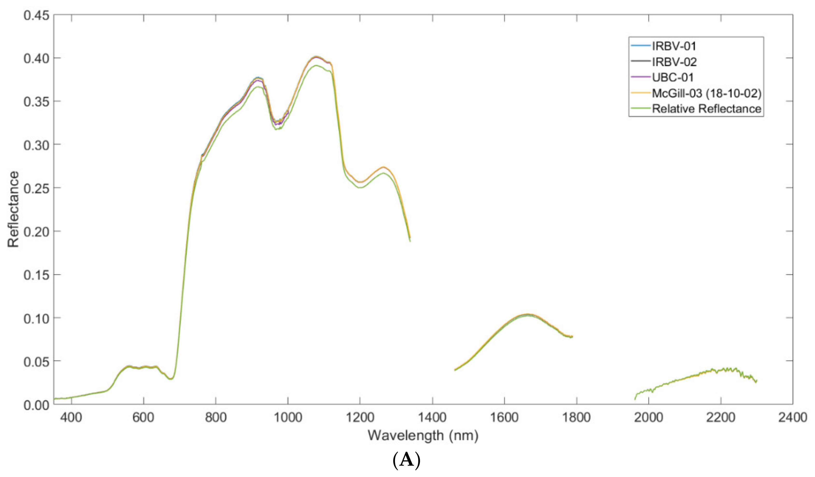
Taking these corrections a step further is to include compensation for the combined direct solar irradiance and anisotropic diffuse sky downwelling irradiance encountered in the field by application of a biconical reflectance factor (BCRF) to the reference panel’s HCRF. This applied BCRF, determined in the laboratory (see [7] for details), is referred to as BCRF(0°:45°) or the R(0°:45°) reflectance factor of the panel (i.e., nadir view: 45° illumination). Due to the known angular dependencies of the reflectance properties of Spectralon®, this R(0°:45°) reflectance factor needs to be adjusted to the observed illumination geometry (assuming a nadir viewing angle) caused by the solar zenith angle (SZA) at the time and location of data acquisition. This normalized BCRF, or nBCRF, is a function of the illumination angle and is wavelength independent [2,18]. The SZA-adjusted nBCRF, nBCRF(SZA), is the specific value at the given illumination angle [10,18]. The nBCRF has been shown to be consistent as a function of wavelength for new and lightly used 99% reflective Spectralon® panels [7,10]. The BCRF(0°:SZA°) can be derived by multiplying BCRF(0°:45°) by nBCRF(SZA), and has been determined to be valid for 99% reflective Spectralon® reference panels used in clear conditions under SZA from near nadir to 60° [18]. Ultimately, this reference panel specific BCRF(0°:SZA°) adjusted Rratio is the estimated Rabs calculated by the toolkit. The significance of these corrections is apparent in Figure 1, which illustrates a vegetation spectrum acquired under an SZA of 42.25°, in which the direct illumination angle differs from the normalization geometry by 2.75°. Through the application of these calculations and adjustments to Rratio, a more accurate estimate of the target’s Rabs is achieved. Details regarding the physical basis for the concepts and the theoretical methodology for the estimation of Rabs can be found in [7,8].
2.2. Overview of the ASD FieldSpec 3 and Data Acquisition
Even though the ASDToolkit was developed for the calculation of Rabs from ASD FieldSpec 3 data, it is not dependent on this specific model of instrument, and is therefore compatible with spectra collected using other models as well. The ASD FieldSpec 3 is composed of three separate internal spectrometers covering a spectral range of 350–2500 nm across the near UV to SWIR regions. Details about the instrument are given in Table 1, as well as in the ASD FieldSpec 3 user manual [19].
2.3. Overview of ASDToolkit
ASDToolkit was created in MATLAB® and consists of a single-window user interface. The toolkit does not require any coding knowledge or coding inputs from the user. It is currently available for the Microsoft Windows operating system. ASDToolkit is launched from the executable file and requires MATLAB® Runtime to be installed. The MATLAB® Runtime installer and instructions are included with the ASDToolkit download package. The fundamental spectroscopy concepts that provide the basis for the processing methodology used by ASDToolkit are discussed at length in [7,8]. These concepts were refined in order to translate effectively into a MATLAB-based processing interface.
2.4. Preparation of ASD Data Files
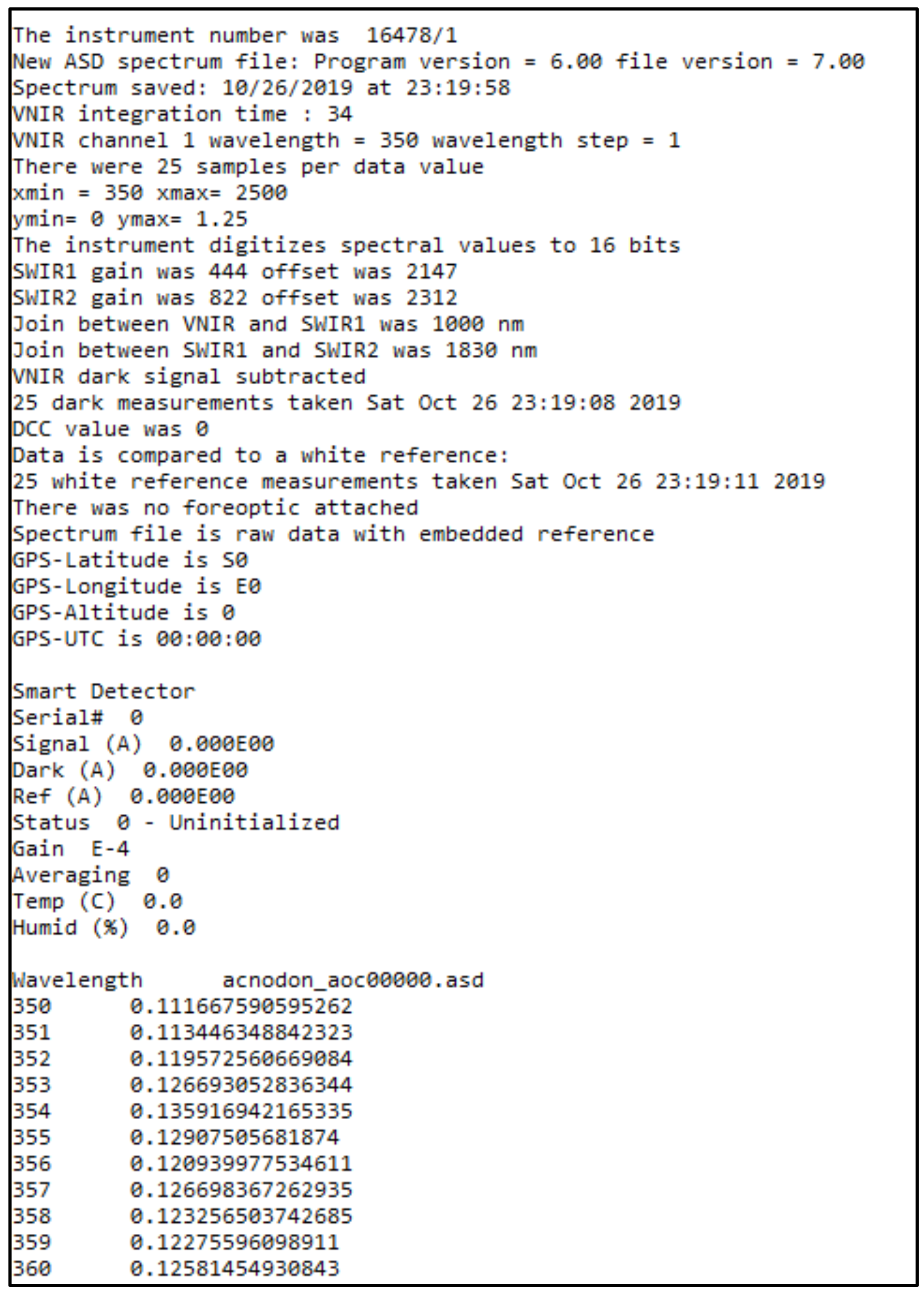
The input format requires ASCII files in which the dark-current-corrected signals in DN have been processed to Rratio. The ASCII file is expected to contain the standard ASD acquisition header information followed by a single spectrum organized as two tab-delimited columns, with the first column containing the wavelength and the second the value of Rratio (Figure 3). A straightforward way to generate these input files is through the freely available software ViewSpecPro, which can be downloaded from Malvern Panalytical [21]. If using ViewSpecPro to generate the input files, they need to be processed using the “ASCII export” option with “Reflectance” selected as the output data format. A detailed user guide on how to correctly pre-process the ASD data files in ViewSpecPro is included with the documentation bundled with the ASDToolkit [22].
2.5. Required User Files
The necessary input files include the Rratio data files (as described in Section 2.4), as well as reference panel characteristic files. Panel characteristic files are ASCII files containing the BCRF(0°:45°) information of the reference panel used to acquire the spectra in the field. The ASDToolkit includes several predefined panels that have been characterized under laboratory conditions by the National Research Council of Canada (NRC) Flight Research Laboratory using the methodology described in [7]. Users have the option of supplying their own panel characteristic file for any panel(s) used in their data collection activities or to capture degradation in the panel reflectance factors that typically occurs over time with use in the field. This is recommended to ensure accuracy of the results. The format of the user-defined panel characteristic file is specific, and requires the following:
- (1)
- The file must be a .csv;
- (2)
- The first row in the first column must contain a panel identifier or panel characteristic file name;
- (3)
- The wavelengths must only be in the first column, beginning at row two;
- (4)
- The panel measurement data must only be in the second column, beginning at row two;
- (5)
- The panel measurements must be provided at the same wavelength intervals as the Rratio files.
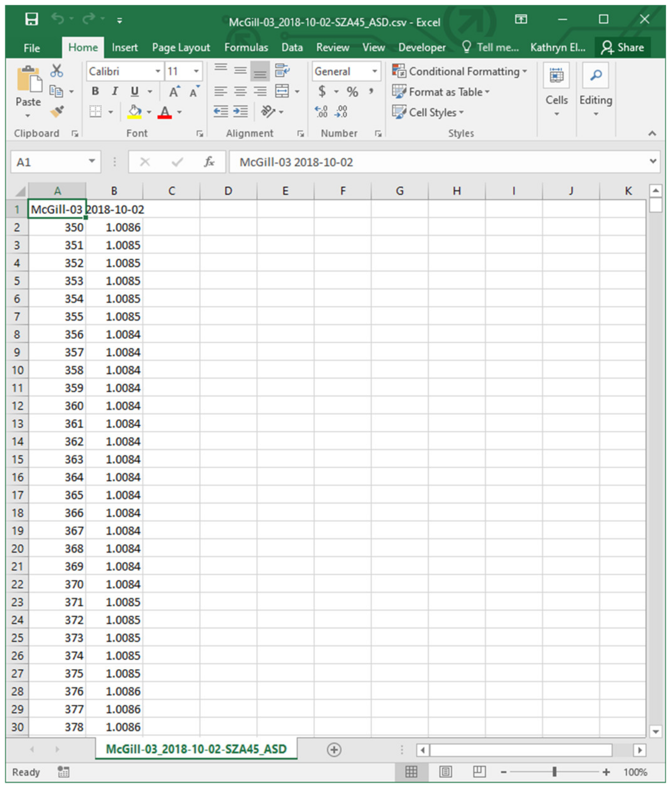
Incorrect formatting will lead to incorrect processing of the data files. An example panel characteristic file is shown in Figure 4, and is provided in the toolkit download package. There are six 99% Spectralon® panels included with ASDToolkit by default. Details of these panels are given in Table 2.
The Rratio files should be contained in a single folder by common latitude/longitude/elevation, as the ASDToolkit assumes a constant location for processing all files contained within the input folder. Changes in latitude/longitude greater than 1 arc-minute or 0.016667 decimal degrees (~1.83 km of linear distance in latitude but varying in longitude) will result in differences in the calculated values for the solar angles, having a noticeable impact on the final result. Therefore, this sensitivity to location means that spectra collected within approximately 1 arc-minute range can be processed together. Spectra collected outside this range should be processed separately to ensure correct solar angle calculations.
2.6. Description of User Inputs to the ASDToolkit Interface
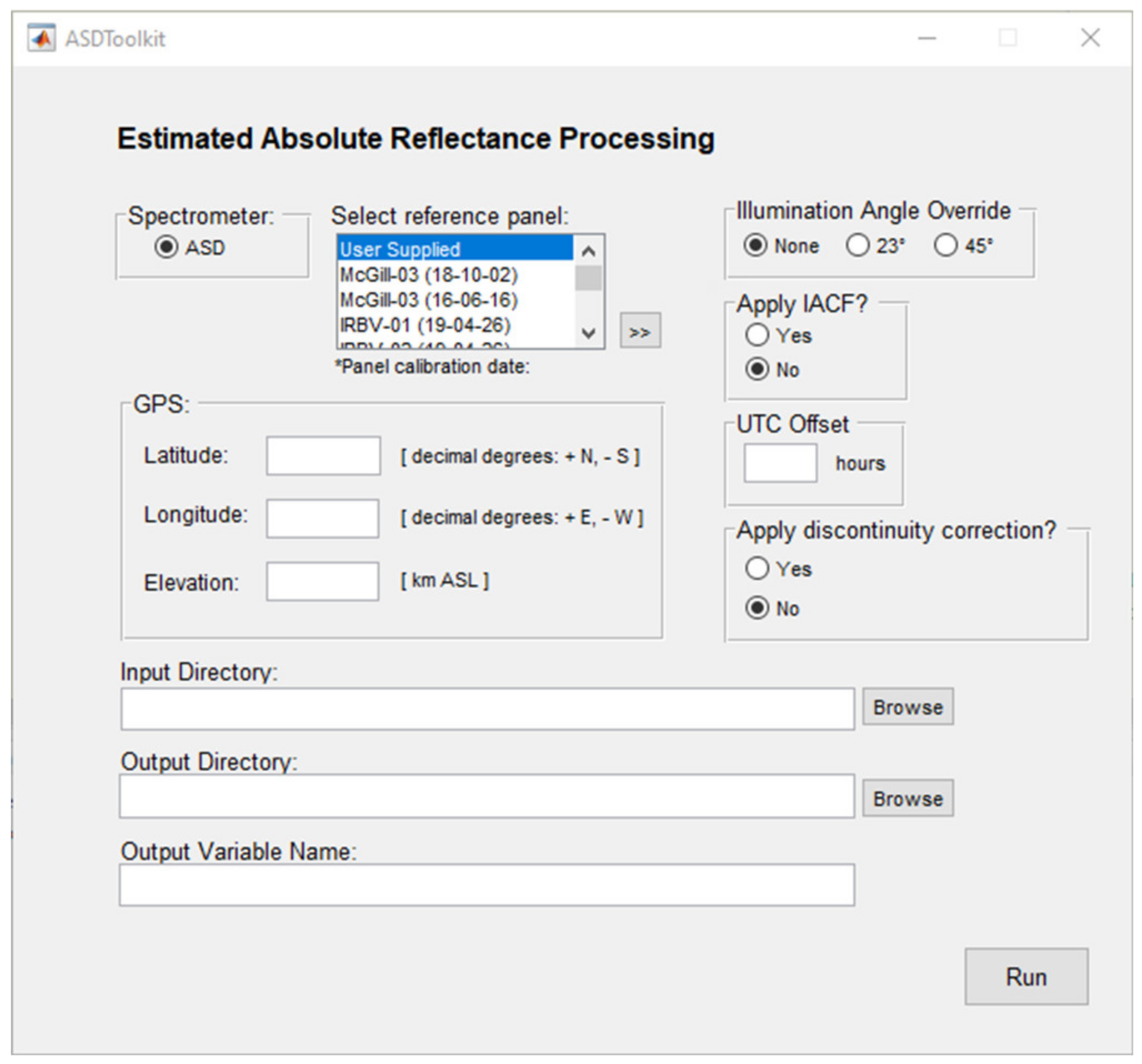
The ASDToolkit user interface (Figure 5) consists of a graphical user interface (GUI) with one main window where the user selects the inputs and processing options. Inputs may be supplied to the appropriate fields in any order; however, all input fields are required. Upon launching the ASDToolkit executable, the user is presented with the main interface window. There are several options for processing Rratio files, including multiple selection choices for the reference panel to use, an option to apply an incident angle correction factor (IACF) to account for the time offset between collection of the reference measurement and target measurements (calculated from the embedded time stamp and provided location coordinates), an option to apply a spectral discontinuity correction at the cross-over wavelengths between the three spectrometers (i.e., 1000 and 1800 nm), and options to override the illumination conditions using two common lab-based illumination and viewing geometries. These options and necessary inputs are described in detail below.
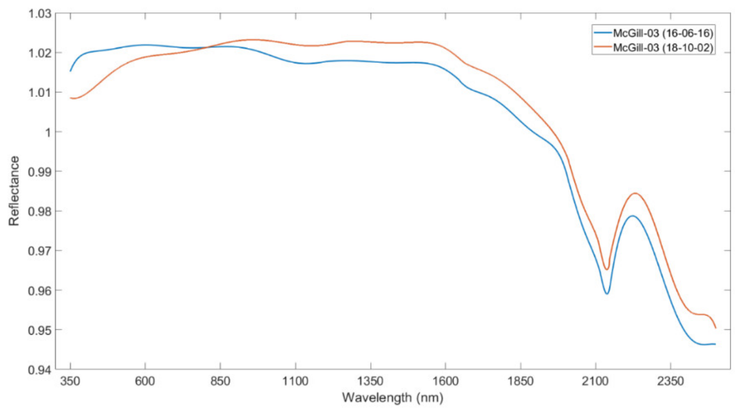
In the “Select Reference Panel” window, the user selects the reference panel to be used for processing. Several panels are included, with the date of calibration given in parentheses appended to the panel name in the list window. Multiple calibrations for a given panel are important if the same panel is used over long periods of time (e.g., years) or suffers excessive degradation due to use. As an example, the two calibrations of the McGill-03 99% Spectralon® panel are shown in Figure 6. To use a reference panel not supplied in the default list, a custom user-provided panel characteristic file must be supplied (as described in Section 2.5). To enable a custom panel, the user should select the “User Supplied” option from the list window. The “>>” button next to the panel list selection is used to set the working directory for the ASDToolkit. It is necessary to leave the working directory as the default path where the ASDToolkit executable is located. Failure to do so will result in the inability of the toolkit to process the files.
The user is required to enter the latitude and longitude (in decimal degrees), as well as elevation (in km above sea level) at which the spectra were acquired. Elevation data are collected for metadata purposes only and are not used in any calculations. For latitude and longitude, North and East are positive (sign not required) and South and West are negative (sign required). The equations and constants to calculate the solar angles are implemented from [8,23] and verified for accuracy against results from [24]. As solar angles are calculated using astronomical algorithms, they do not require a specific horizontal or vertical datum. The number of hours offset from Universal Time Coordinated (UTC) based on the time zone applied to the embedded time stamp must also be entered. For example, Eastern Standard Time has an offset of −4 h from UTC during the months of March to November (accounting for daylight standard time) and an offset of −5 h from UTC during December to February. Using the entered offset, the toolkit converts the collection time found in the Rratio file headers to UTC for processing.
The ASDToolkit provides the option to override the illumination (i.e., elevation and azimuth) calculated using solar angle geometry based on the latitude/longitude at which the spectra were acquired. Overriding the illumination calculation sets the viewing:illumination geometry to 0°:45°, or 0°:23°, the standard time-independent geometries encountered in a laboratory setting and when acquiring spectra with the ASD contact probe accessory respectively. For data collected in the field under natural solar illumination conditions, this override option should be set to “None” so that the illumination geometry is calculated.
Another processing option is whether an incident angle correction factor (IACF) [7] is applied to account for systematic variances in the downwelling irradiance conditions due to progression in the solar geometry between the acquisition times of the reference panel and target measurement. If the reference measurement and target measurement are acquired close together in time, the effect of the IACF will be minimal. However, if enough time has elapsed between collection of the reference measurement and target measurement(s), the IACF calculates a correction factor by taking the cosine of the solar zenith angle for the reference measurement divided by the cosine of the solar zenith angle for the target measurement. Benefits of this correction under natural solar illumination conditions have been shown to be evident for periods of time as short as 5 min (see Figure 12 of [7]). The IACF is calculated using Equation (2):
where is the calculated solar zenith angle (degrees) at the time that the reference measurement was collected, and is the calculated solar zenith angle (degrees) at the time that the target measurement was collected. Once the IACF has been calculated, it is then used to scale the associated spectral reflectance values for each individual file prior to application. ASDToolkit provides output files containing both the estimated Rabs and the estimated Rabs with the IACF applied for user comparison. Additionally, a column containing the individual IACF values for each processed file’s individual timestamp is included in the output MATLAB® structure.
The ASD FieldSpec spectrometers have known spectral discontinuities originating from multiple potential sources [19,25,26,27] and may result in spectral “steps” in the reflectance values at the wavelength thresholds between the three internal spectrometers, namely, 1000 nm and 1800 nm. Certain conditions may cause these discontinuities to become more or less pronounced. The VNIR fiber bundle has a slightly broader FOV than those of the two SWIR instruments (see Figure 4 in [27]). Therefore, one of the most common causes for the discontinuities in the reflectance is due to shading differences between the VNIR and SWIR data, leading to differences in the radiance measured by each detector [19]. Excessive discontinuities are due to other factors such as use of the instrument prior to achieving thermal stability following power on, which can be of significant duration (an hour or longer) under extreme and rapid temperature changes. The use of a lens to reduce the FOV with heterogeneous or specular targets can also result in exaggerated discontinuities. ViewSpecPro contains an option for a “parabolic correction” to mitigate these discontinuities [19]. If it is not applied, a processing option is included in this toolkit to apply a “discontinuity correction” to the data [28]. It is important to note that the calculation of the discontinuity correction solutions performed by the toolkit is based on estimating the gradient between the edges of the discontinuity and calculating an additive and multiplicative solution to blend the two edges of the discontinuity together, rather than calculating a solution based on a specific empirical model. If the discontinuity correction option is selected, these solutions are provided in additional files separate from the original processed spectra so that the user can evaluate the results.
Lastly, the user must select the input directory, which is the folder that contains the Rratio files (pre-processed as per Section 2.4). The selected output directory is where all the generated results files will be saved. Both the input and output file directories may be selected by clicking the associated “Browse” button, or the full path name can be entered into the user input box. The output variable name is the root file name that all the processed files will share, with additional file naming conventions appended automatically such as “*_estimatedAbsoluteReflectance,” “*_headerInfo,” “*_estimatedAbsoluteReflectance_IACF,” and others (see Section 3.2).
Once the user has entered the required inputs, the toolkit can then be executed. If there are any errors in the inputs, such as improper latitude/longitude data, blank fields, invalid file types, or invalid directories, then specific error messages will appear that detail which error occurred and the changes to the inputs required to resolve the error. The user can close the error message window and fix the erroneous inputs as necessary and proceed to run the toolkit again without needing to completely re-enter all the other inputs. If the user selected the “User Supplied” option in the panel list, then a new window will open prompting the user to navigate to the correct directory and select the custom user-defined panel characteristic file. If one of the pre-defined panels is selected, the toolkit will begin to process the selected data files immediately, and a progress bar will appear during processing. Once the processing is complete, a message will be displayed on the screen that indicates the processing has been completed successfully. The user may then navigate away from the ASDToolkit interface (either minimizing or completely closing the interface window) to the output directory and locate the output files. A video walk-through of the ASDToolkit is shown in Supplementary Video 1.
3. Methodology
3.1. ASDToolkit Workflow
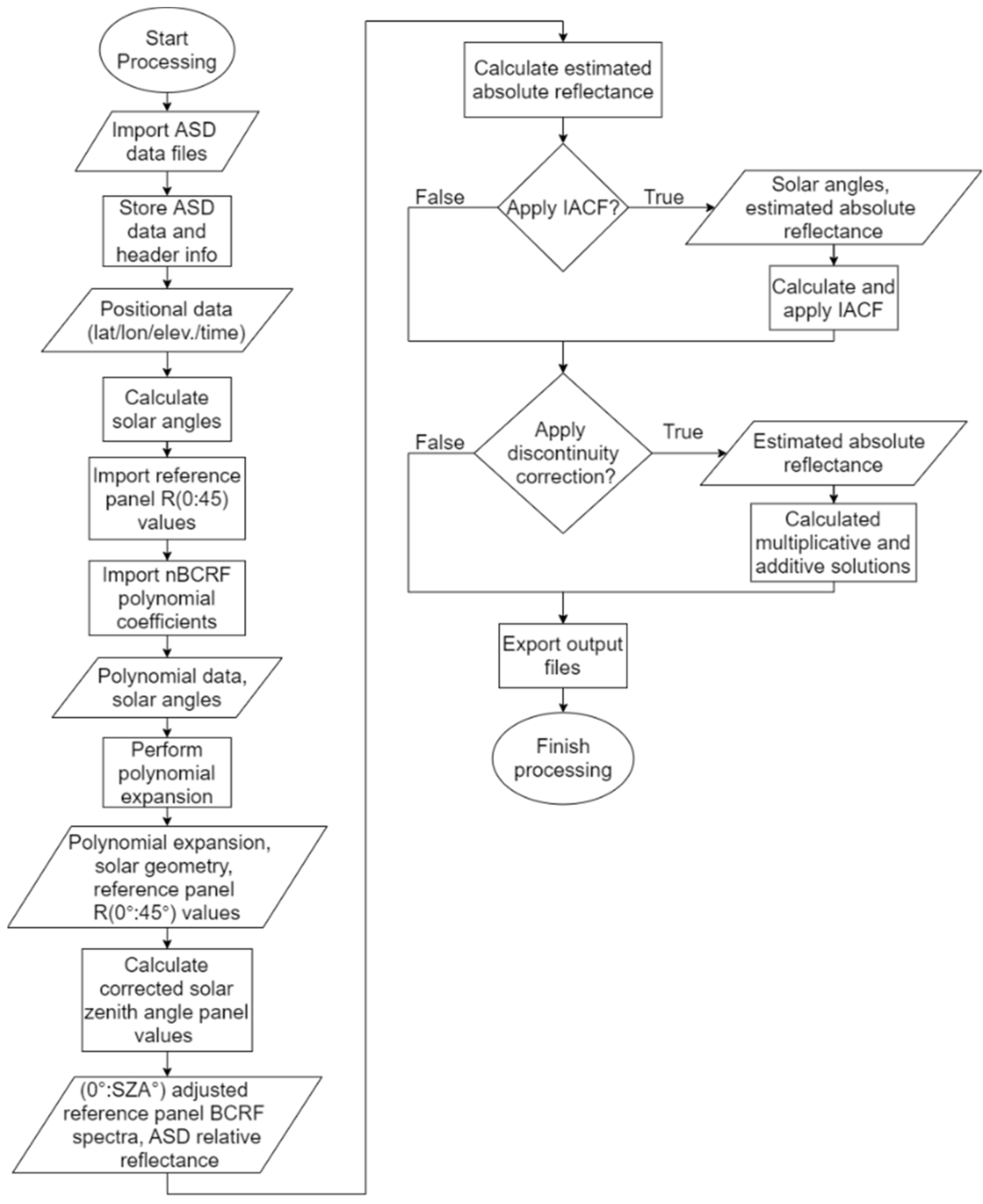
The internal processing workflow is shown in detail in Figure 7 and described below.
- Import necessary reflectance files [29]
- Inputs: ASD data files;
- Outputs: ASD relative reflectance data, header information (time, date, wavelength, etc.).
- Calculate the solar zenith angles
- Inputs: ASD data file header information (date, time), latitude/longitude information, hours offset from UTC;
- Outputs: Solar azimuth angle, solar zenith angle.
- Import panel-specific values for R(0°:45°)
- Inputs: Reference panel characteristic files (pre-defined or user supplied);
- Outputs: Panel characteristic information.
- Import nBCRF polynomial coefficients
- Inputs: Panel-independent BCRF (0°:45°);
- Outputs: nBCRF polynomial parameters.
- Polynomial expansion
- Inputs: Panel-specific BCRF (0°:45°), solar geometry data, nBCRF polynomial parameters;
- Outputs: Polynomial expansion results adjusted for normalized BCRF.
- Calculate the corrected solar zenith angle panel values
- Inputs: Average polynomial expansion results, solar geometry data;
- Outputs: (0°:SZA°) adjusted reference panel BCRF spectra for the given panel.
- Calculate estimated absolute reflectance
- Inputs: SZA-adjusted panel BCRF, ASD relative reflectance data;
- Outputs: Estimated absolute reflectance values.
- Apply IACF or not
- Inputs: Solar zenith angle of reference measurement, solar zenith angle of target measurement;
- Outputs: Estimated absolute reflectance values with IACF applied.
- Apply discontinuity correction
- Inputs: Estimated absolute reflectance values;
- Outputs: Estimated absolute reflectance values with correction applied.
- Export results
- Inputs: Estimated absolute reflectance data structure;
- Outputs: Header file, estimated absolute reflectance data structure (as a MATLAB file and an Excel file), IACF file, discontinuity correction files (additive and multiplicative solutions).
3.2. ASDToolkit Output Files
Depending on the processing options selected in the interface window, optional output files may be generated. Files that are always generated are:
- variablename.mat: A MATLAB® (*.mat) data file that contains all the processed data and header information and can be opened directly in MATLAB® for further data manipulation.
- variablename_estimatedAbsoluteReflectance.csv: A (*.csv) file that contains the estimated absolute reflectance output values where each column represents a single data file, with the name of the file as the first row in each column.
- variablename_headerInfo.csv: A (*.csv) file that contains the detailed header information for each processed file, where each column represents a single data file that was processed.
Optional files that are generated based on the selected processing options are:
- variablename_estimatedAbsoluteReflectance_IACF.csv: Generated when the IACF option is selected in the interface. A (*.csv) file that contains the estimated absolute reflectance output values with the IACF applied, where each column represents a single data file, with the name of the file as the first row in each column.
- variablename_DC_additive.csv: Generated when the Discontinuity Correction option is selected in the interface. A (*.csv) file that contains the estimated absolute reflectance values for the additive solution, where each column represents a single data file, with the name of the file as the first row in each column.
- variablename_DC_multiplicative.csv: Generated when the Discontinuity Correction option is selected in the interface. A (*.csv) file that contains the estimated absolute reflectance values for the multiplicative solution, where each column represents a single data file, with the name of the file as the first row in each column.
3.3. Details on the Generated MATLAB® Data File (*.mat)
As described in Section 3.2, one of the output files that is always generated is the MATLAB® data file (*.mat), which is named using the input variable name entered in the interface window. The generated file can be loaded and executed directly in the MATLAB® workspace using the command line in MATLAB® and the following command:
where “outputVariableName” is the variable name entered in the interface. It is important to note that in order to successfully load the (*.mat) file into MATLAB® using the above command, the current folder or MATLAB® path must be set to the folder that contains the (*.mat) file. Once loaded into the workspace, the variable name will default to “estimatedAbsoluteReflectance.” The user is also able to import the data structure to MATLAB® using a different initial variable name using the command:
where “dataStructure” will be the name of the variable in the MATLAB® workspace. It is necessary to load the (*.mat) data file with a unique name in the workspace when processing multiple sets of files and subsequently opening the multiple generated (*.mat) files, as each variable will have an automatic variable name of “estimatedAbsoluteReflectance” in the workspace.
The MATLAB® data structure contains 18 fields if all options are enabled in the interface, and they are listed and described in Table 3.
4. User Notes
Detailed documentation is provided along with the ASDToolkit download from http://0-doi-org.brum.beds.ac.uk/10.5281/zenodo.3996377. The documents provided include a guide on how to correctly prepare the ASD data files using ViewSpecPro software (to output Rratio), a user guide containing the steps to use the interface, as well as details regarding the output files. Images of sample files such as a sample user-defined panel characteristic file are included within the user guide to serve as a visual reference for user files. An actual sample panel characteristic file is also included, as it is critical that any user-supplied panel characteristic files must match the example formatting.
5. Conclusions
In situ field or ground reflectance measurements form an important dataset in remote sensing studies; however, Rabs is not measured directly by field spectrometers and therefore must be calculated. ASDToolkit, a novel MATLAB® processing toolkit, allows for a simple and straightforward batch processing of FieldSpec field spectroscopy data files in order to generate Rabs from the Rratio. By creating a linear workflow and using an easy to understand GUI with supporting documentation, users are able to repeatedly process multiple datasets of different sizes collected under various conditions in an efficient manner with traceable results. The files generated by the toolkit are available for further use within MATLAB® and as .csv files and are therefore readily converted to different file types dependent upon user requirements.
Supplementary Materials
The following are available online at https://0-www-mdpi-com.brum.beds.ac.uk/2306-5729/5/4/96/s1, Video S1: ASDToolkit_demo_processingSteps.mp4.
Author Contributions
Conceptualization, R.J.S. and J.P.A.-M.; methodology, R.J.S.; software, K.E.; writing—Original draft preparation, K.E., R.J.S., and M.K.; writing—Review and editing, K.E., R.J.S., M.K., and J.P.A.-M. All authors have read and agreed to the published version of the manuscript.
Funding
This research was funded by the National Research Council of Canada (NRC) and a Natural Sciences and Engineering Research Council (NSERC) Discovery Frontiers grant that supported the Canadian Airborne Biodiversity Observatory (CABO). The APC was funded by an NSERC Discovery Grant (to Kalacska).
Acknowledgments
We would like to acknowledge the efforts of Erica Skye Schaaf, who rigorously tested and provided feedback on the ASDToolkit throughout its development. We thank Etienne Laliberté (Université de Montréal) and Nicholas Coops (UBC) for provision of their reference panels through CABO for inclusion in the toolkit.
Conflicts of Interest
The authors declare no conflicts of interest. The funders had no role in the design of the study; in the collection, analyses, or interpretation of data; in the writing of the manuscript; or in the decision to publish the results.
References
- Milton, E. Review article principles of field spectroscopy. Remote Sens. 1987, 8, 1807–1827. [Google Scholar] [CrossRef]
- Milton, E.J.; Schaepman, M.E.; Anderson, K.; Kneubühler, M.; Fox, N. Progress in field spectroscopy. Remote Sens. Environ. 2009, 113, S92–S109. [Google Scholar] [CrossRef] [Green Version]
- Hueni, A.; Damm, A.; Kneubuehler, M.; Schläpfer, D.; Schaepman, M.E. Field and airborne spectroscopy cross validation—Some considerations. IEEE J. Sel. Top. Appl. Earth Obs. Remote Sens. 2016, 10, 1117–1135. [Google Scholar] [CrossRef]
- Majeke, B.; Van Aardt, J.; Cho, M. Imaging spectroscopy of foliar biochemistry in forestry environments. South. For. A J. For. Sci. 2008, 70, 275–285. [Google Scholar] [CrossRef]
- Shapira, U.; Herrmann, I.; Karnieli, A.; Bonfil, D.J. Field spectroscopy for weed detection in wheat and chickpea fields. Int. J. Remote Sens. 2013, 34, 6094–6108. [Google Scholar] [CrossRef] [Green Version]
- Choe, E.; van der Meer, F.; van Ruitenbeek, F.; van der Werff, H.; de Smeth, B.; Kim, K.-W. Mapping of heavy metal pollution in stream sediments using combined geochemistry, field spectroscopy, and hyperspectral remote sensing: A case study of the Rodalquilar mining area, SE Spain. Remote Sens. Environ. 2008, 112, 3222–3233. [Google Scholar] [CrossRef]
- Soffer, R.J.; Ifimov, G.; Arroyo-Mora, J.P.; Kalacska, M. Validation of Airborne Hyperspectral Imagery from Laboratory Panel Characterization to Image Quality Assessment: Implications for an Arctic Peatland Surrogate Simulation Site. Can. J. Remote Sens. 2019, 45, 476–508. [Google Scholar] [CrossRef]
- Peddle, D.R.; White, H.P.; Soffer, R.J.; Miller, J.R.; Ledrew, E.F. Reflectance processing of remote sensing spectroradiometer data. Comput. Geosci. 2001, 27, 203–213. [Google Scholar] [CrossRef]
- Gatebe, C.K.; King, M.D. Airborne spectral BRDF of various surface types (ocean, vegetation, snow, desert, wetlands, cloud decks, smoke layers) for remote sensing applications. Remote Sens. Environ. 2016, 179, 131–148. [Google Scholar] [CrossRef]
- Jackson, R.D.; Clarke, T.R.; Moran, M.S. Bidirectional calibration results for 11 Spectralon and 16 BaSO4 reference reflectance panels. Remote Sens. Environ. 1992, 40, 231–239. [Google Scholar] [CrossRef]
- Sandmeier, S.R. Acquisition of bidirectional reflectance factor data with field goniometers. Remote Sens. Environ. 2000, 73, 257–269. [Google Scholar] [CrossRef]
- Georgiev, G.T.; Butler, J.J.; Cooksey, C.; Ding, L.; Thome, K.J. SWIR calibration of spectralon reflectance factor. In Sensors, Systems, and Next-Generation Satellites XV; International Society for Optics and Photonics: Bellingham, WA, USA, 2011; Volume 8176, p. 81760W. [Google Scholar]
- Williams, D.C. Establishment of absolute diffuse reflectance scales using the NPL Reference Reflectometer. Anal. Chim. Acta 1999, 380, 165–172. [Google Scholar] [CrossRef]
- Bruegge, C.J.; Stiegman, A.E.; Coulter, D.R.; Hale, R.R.; Diner, D.J.; Springsteen, A.W. Reflectance stability analysis of Spectralon diffuse calibration panels. In Calibration of Passive Remote Observing Optical and Microwave Instrumentation; International Society for Optics and Photonics: Bellingham, WA, USA, 1991; Volume 1493, pp. 132–142. [Google Scholar]
- Möller, W.; Nikolaus, K.; Höpe, A. Degradation of the diffuse reflectance of Spectralon under low-level irradiation. Metrologia 2003, 40, S212. [Google Scholar] [CrossRef]
- Stiegman, A.E.; Bruegge, C.J.; Springsteen, A.W. Ultraviolet stability and contamination analysis of Spectralon diffuse reflectance material. Opt. Eng. 1993, 32, 799–805. [Google Scholar] [CrossRef] [Green Version]
- Sun, J.; Chu, M.; Wang, M. Degradation nonuniformity in the solar diffuser bidirectional reflectance distribution function. Appl. Opt. 2016, 55, 6001–6016. [Google Scholar] [CrossRef] [PubMed]
- Rollin, E.; Milton, E.; Emery, D. Reference panel anisotropy and diffuse radiation-some implications for field spectroscopy. Int. J. Remote Sens. 2000, 21, 2799–2810. [Google Scholar] [CrossRef]
- Devices, A.S. FieldSpec 3 User Manual. ASD Doc. 2010, 600540, 92. [Google Scholar]
- Kalacska, M.; Arroyo-Mora, J.P.; Soffer, R.; Elmer, K. ASD FieldSpec 3 Field Measurement Protocols. Available online: Dx.doi.org/10.17504/protocols.io.qu7dwzn (accessed on 8 September 2019).
- Malvern Panalytical. ViewSpec Pro Software Install. Available online: https://www.malvernpanalytical.com/en/support/product-support/software/ViewSpecProSoftwareInstall.html (accessed on 4 September 2016).
- Elmer, K.; Soffer, R.; Arroyo-Mora, J.P.; Kalacska, M. 2020 ASDToolkit: A Novel MATLAB Processing Toolbox for ASD Field Spectroscopy Data (Software). Zenodo. Available online: https://0-doi-org.brum.beds.ac.uk/10.5281/ZENODO.3996377 (accessed on 16 February 2018).
- U. S. Naval Observatory; U.K.H.O.; H.M. Nautical Almanac Office. The Astronomical Almanac for the Year 2015. U.S. Govt. Printing Office: Washington, DC, USA, 2015. [Google Scholar]
- Cornwall, C.; Horiuchi, A.; Lehman, C. NOAA Solar Position Calculator. 2020. Available online: http://www.esrl.noaa.gov/gmd/grad/solcalc/azel.html (accessed on 31 August 2017).
- Hueni, A.; Bialek, A. Cause, effect, and correction of field spectroradiometer interchannel radiometric steps. IEEE J. Sel. Top. Appl. Earth Obs. Remote Sens. 2017, 10, 1542–1551. [Google Scholar] [CrossRef]
- Hemmer, T.H.; Westphal, T.L. Lessons learned in the postprocessing of field spectroradiometric data covering the 0.4-2.5-um wavelength region. In Algorithms for Multispectral, Hyperspectral, and Ultraspectral Imagery VI; International Society for Optics and Photonics: Bellingham, WA, USA, 2000; Volume 4049, pp. 249–260. [Google Scholar]
- Mac Arthur, A.; MacLellan, C.J.; Malthus, T. The fields of view and directional response functions of two field spectroradiometers. Ieee Trans. Geosci. Remote Sens. 2012, 50, 3892–3907. [Google Scholar] [CrossRef]
- Karami, M. asd_jumpcorrection. Available online: https://github.com/mkarami/Karami-2013/blob/master/asd_jumpcorrection.m (accessed on 16 February 2018).
- Robinson, I. Field Spectroscopy Facility Post Processing Toolbox, 1.3.1; MATLAB Central File Exchange; MathWorks: Natick, MA, USA, 2011. [Google Scholar]
Figure 1.
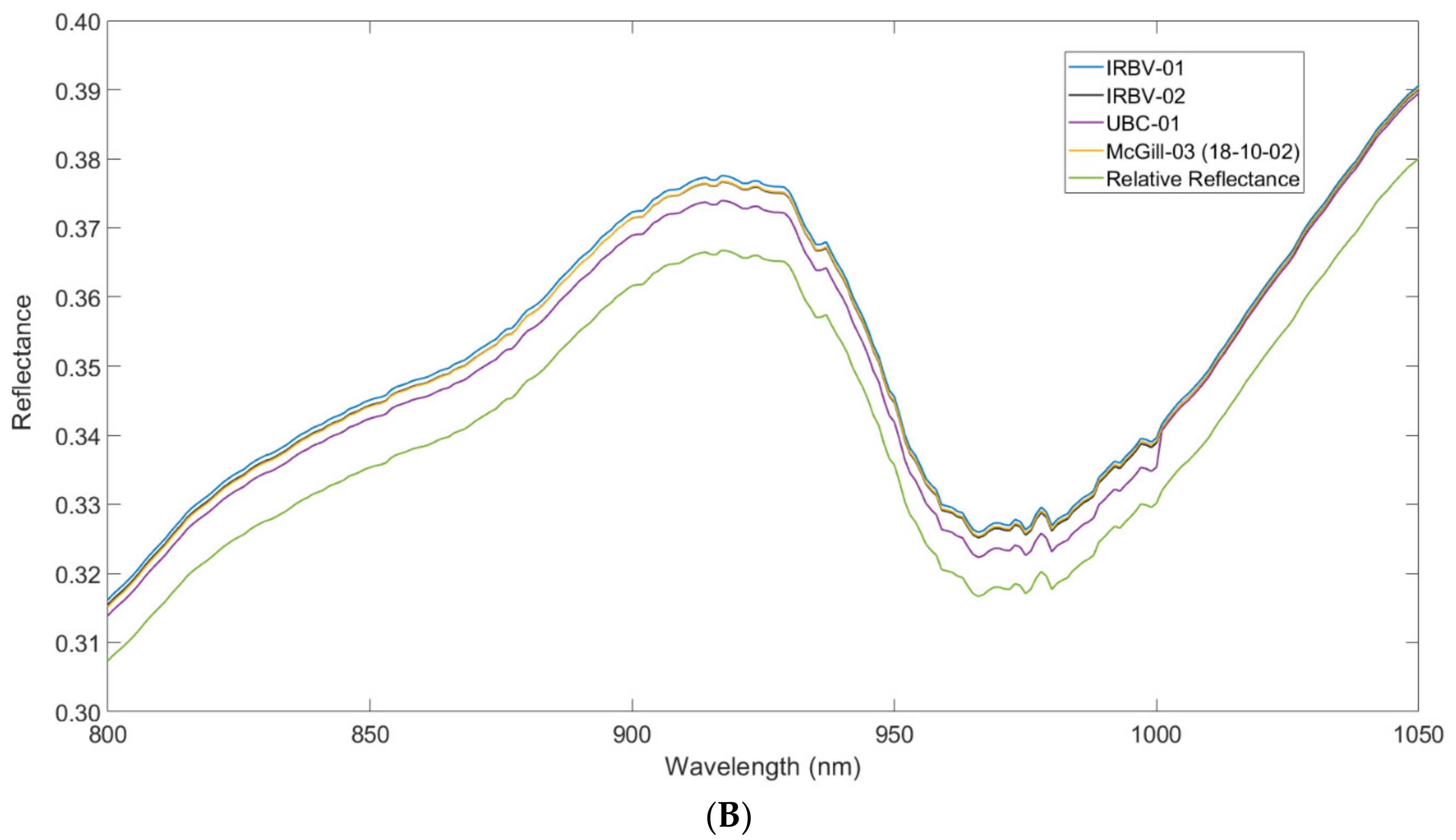
Example of estimated Rabs calculated by the toolkit. Spectra are of vegetation acquired under a solar zenith angle (SZA) of 42.25°. It is important to note that the difference between Rratio (relative reflectance) and estimated Rabs will vary as a function of the SZA. (A) Comparison of Rratio and Rabs as estimated using the BCRF(0°:45°) of four different 99% Spectralon® panels of various ages: McGill-03, IRBV-01, IRBV-02, and UBC-01. The actual panel used in the field during data acquisition of this spectrum was McGill-03, making this the best estimate of Rabs. (B) An enlargement of spectrum from (A) over the 800–1050 nm range, illustrating the impact of calculating estimated Rabs from Rratio using different panels.
Figure 1.
Example of estimated Rabs calculated by the toolkit. Spectra are of vegetation acquired under a solar zenith angle (SZA) of 42.25°. It is important to note that the difference between Rratio (relative reflectance) and estimated Rabs will vary as a function of the SZA. (A) Comparison of Rratio and Rabs as estimated using the BCRF(0°:45°) of four different 99% Spectralon® panels of various ages: McGill-03, IRBV-01, IRBV-02, and UBC-01. The actual panel used in the field during data acquisition of this spectrum was McGill-03, making this the best estimate of Rabs. (B) An enlargement of spectrum from (A) over the 800–1050 nm range, illustrating the impact of calculating estimated Rabs from Rratio using different panels.


Figure 2.
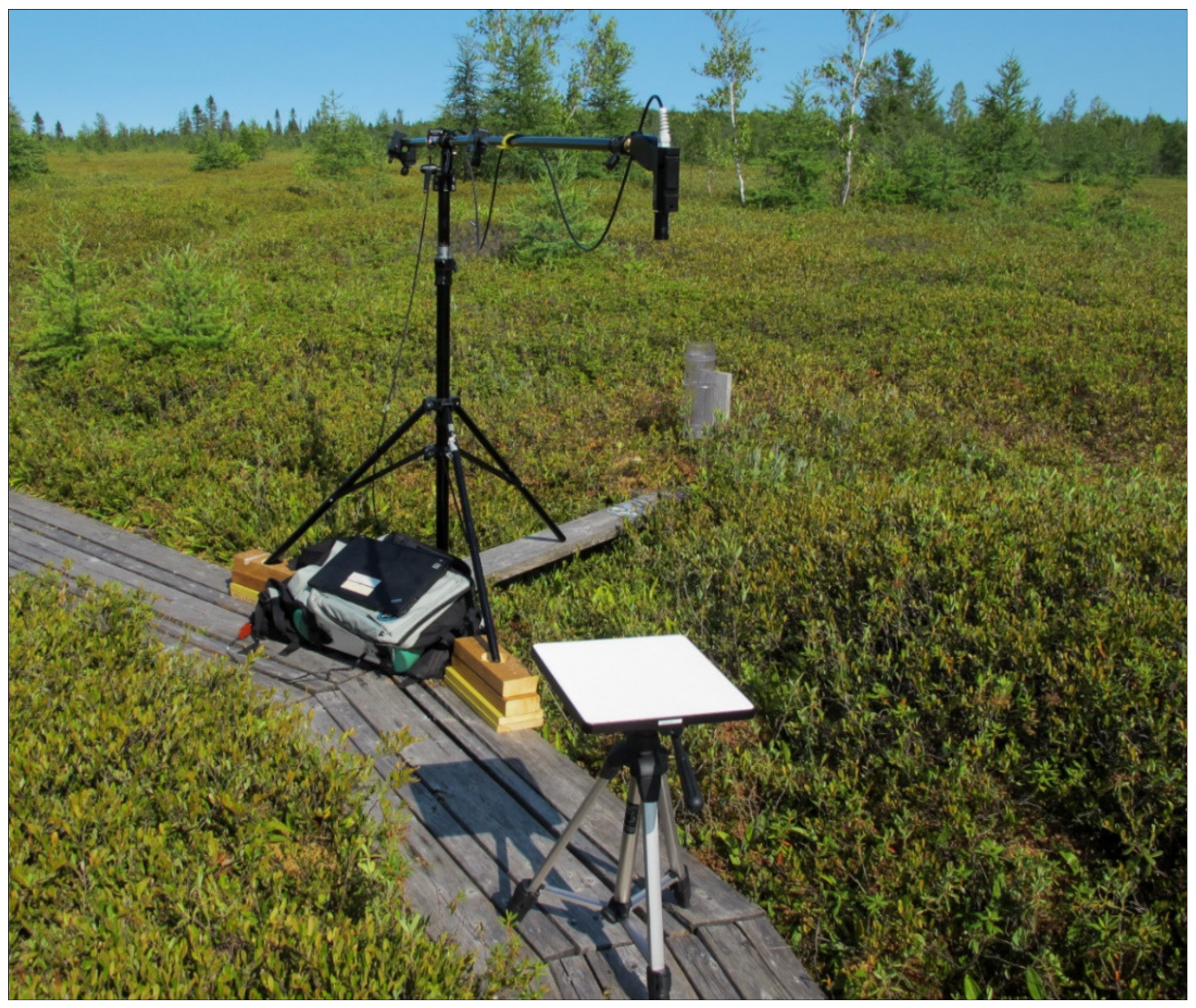
An example of the ASD FieldSpec 3 instrument setup in the field for data acquisition using a tripod, the fiberoptic cable extension, pistol grip, and a 99% Spectralon panel as white reference.
Figure 2.
An example of the ASD FieldSpec 3 instrument setup in the field for data acquisition using a tripod, the fiberoptic cable extension, pistol grip, and a 99% Spectralon panel as white reference.

Figure 3.
Example of the expected format of an ASCII file for input to the toolkit. Only wavelengths 350–360 nm are shown. This file of Rratio was generated in ViewSpecPro.
Figure 3.
Example of the expected format of an ASCII file for input to the toolkit. Only wavelengths 350–360 nm are shown. This file of Rratio was generated in ViewSpecPro.

Figure 4.
Example of the expected format of a panel characteristic file. Only wavelengths 350–378 nm are shown.
Figure 4.
Example of the expected format of a panel characteristic file. Only wavelengths 350–378 nm are shown.

Figure 5.
Main interface window where the user selects the inputs and processing options.

Figure 6.
Degradation of the McGill-03 99% reflective Spectralon® panel between two calibration dates (16 June 2016 and 2 October 2018).
Figure 6.
Degradation of the McGill-03 99% reflective Spectralon® panel between two calibration dates (16 June 2016 and 2 October 2018).

Figure 7.
Flowchart of the internal processing workflow of the toolkit.


Table 1.
Primary specifications of the ASD FieldSpec 3. FWHM refers to the full-width-half-maximum.
| Characteristic | Range |
|---|---|
| Spectral range | VNIR: 350–1050 nm |
| SWIR1: 1000–1800 nm | |
| SWIR2: 1800–2500 nm | |
| Spectral resolution | 3 nm FWHM at 700 nm |
| 10 nm FWHM at 1400 and 2100 nm | |
| Sampling interval | 1.4 nm at 350–1050 nm |
| 2 nm at 1000–2500 nm | |
| No. of optical fibers | VNIR: 19 fibers (100 µm) |
| SWIR1-2: 38 fibers (200 µm) |
Table 2.
Details of 99% Spectralon® reference panels included with the ASDToolkit.
| Panel Identifier | Original (8°:h) Calibration | NRC 0°:45° Calibration Date(s)(yy-mm-dd) | Usage Type |
|---|---|---|---|
| IRBV-01 | June 2018 | 19-04-26 | Field use |
| IRBV-02 | June 2018 | 19-04-26 | New |
| McGill-03 | March 2013 | 18-10-02 16-06-16 | Field use |
| NRC-01 | March 2011 | 16-06-17 | Field use |
| NRC-02 | February 2012 | 16-06-16 | Primary lab 2012–2016 Field use 2016–ongoing |
| UBC-01 | June 2006 | 19-04-26 | Field use |
Table 3.
A list and descriptions of the fields in the MATLAB data structure variable.
| Field Name | Description |
|---|---|
| path | Directory path of the input files |
| name | Name of the input files |
| header | Original ASD header information for the imported files |
| datetime | Date and time information for the imported files |
| panel | Filename of panel characteristic file |
| latitude | Input latitude value |
| longitude | Input longitude value |
| elevation | Input elevation value |
| reference_zenith | Calculated solar zenith angle for the reference measurement |
| reference_azimuth | Calculated solar azimuth angle for the reference measurement |
| target_zenith | Calculated solar zenith angle for the target measurement |
| target_azimuth | Calculated solar azimuth angle for the target measurement |
| wavelength | An array of type “Double” that contains the wavelength intervals for the imported files |
| reflectance | An array of type “Double” that contains the estimated absolute reflectance values for the imported files |
| IACF | Calculated IACF value for a given file |
| IACF_reflectance | An array of type “Double” that contains the estimated absolute reflectance values with the IACF applied |
| DC_additive | An array of type “Double” that contains the additive solution for the ASD discontinuity correction |
| DC_multiplicative | An array of type “Double” that contains the multiplicative solution for the ASD discontinuity correction |
© 2020 by the authors. Licensee MDPI, Basel, Switzerland. This article is an open access article distributed under the terms and conditions of the Creative Commons Attribution (CC BY) license (http://creativecommons.org/licenses/by/4.0/).
Share and Cite
MDPI and ACS Style
Elmer, K.; Soffer, R.J.; Arroyo-Mora, J.P.; Kalacska, M. ASDToolkit: A Novel MATLAB Processing Toolbox for ASD Field Spectroscopy Data. Data 2020, 5, 96. https://0-doi-org.brum.beds.ac.uk/10.3390/data5040096
AMA Style
Elmer K, Soffer RJ, Arroyo-Mora JP, Kalacska M. ASDToolkit: A Novel MATLAB Processing Toolbox for ASD Field Spectroscopy Data. Data. 2020; 5(4):96. https://0-doi-org.brum.beds.ac.uk/10.3390/data5040096
Chicago/Turabian StyleElmer, Kathryn, Raymond J. Soffer, J. Pablo Arroyo-Mora, and Margaret Kalacska. 2020. "ASDToolkit: A Novel MATLAB Processing Toolbox for ASD Field Spectroscopy Data" Data 5, no. 4: 96. https://0-doi-org.brum.beds.ac.uk/10.3390/data5040096