
Agricultural Crop Change in the Willamette Valley, Oregon, from 2004 to 2017


1
College of Forestry, Oregon State University, Corvallis, OR 97333, USA
2
National Forage Seed Production Research Center, USDA-Agricultural Research Service, Corvallis, OR 97333, USA
*
Author to whom correspondence should be addressed.
†
Retired.
Data 2021, 6(2), 17; https://0-doi-org.brum.beds.ac.uk/10.3390/data6020017
Submission received: 23 December 2020
/
Revised: 2 February 2021
/
Accepted: 4 February 2021
/
Published: 7 February 2021
(This article belongs to the Section Spatial Data Science and Digital Earth)
Abstract
:The Willamette Valley, bounded to the west by the Coast Range and to the east by the Cascade Mountains, is the largest river valley completely confined to Oregon. The fertile valley soils combined with a temperate, marine climate create ideal agronomic conditions for seed production. Historically, seed cropping systems in the Willamette Valley have focused on the production of grass and forage seeds. In addition to growing over two-thirds of the nation’s cool-season grass seed, cropping systems in the Willamette Valley include a diverse rotation of over 250 commodities for forage, seed, food, and cover cropping applications. Tracking the sequence of crop rotations that are grown in the Willamette Valley is paramount to answering a broad spectrum of agronomic, environmental, and economical questions. Landsat imagery covering approximately 25,303 km2 were used to identify agricultural crops in production from 2004 to 2017. The agricultural crops were distinguished by classifying images primarily acquired by three platforms: Landsat 5 (2003–2013), Landsat 7 (2003–2017), and Landsat 8 (2013–2017). Before conducting maximum likelihood remote sensing classification, the images acquired by the Landsat 7 were pre-processed to reduce the impact of the scan line corrector failure. The corrected images were subsequently used to classify 35 different land-use classes and 137 unique two-year-long sequences of 57 classes of non-urban and non-forested land-use categories from 2004 through 2014. Our final data product uses new and previously published results to classify the western Oregon landscape into 61 different land use classes, including four majority-rule-over-time super-classes and 57 regular classes of annually disturbed agricultural crops (19 classes), perennial crops (20 classes), forests (13 classes), and urban developments (5 classes). These publicly available data can be used to inform and support environmental and agricultural land-use studies.
Data Set License: CC-BY-4.0
1. Introduction
Remote sensing of the Earth provides an unimaginable wealth of data about our planet. However, the images are rarely used in their raw form; rather, they are generally interpreted using various analytical techniques. Landsat is the satellite program that earned a preeminent place in Earth surveying. The Landsat program (i.e., first launched in 1972) has provided uninterrupted coverage of the Earth; an area is observed approximately every 16 days with a current spatial resolution of 15 or 30 m. However, Landsat sensors have not always operated as expected, such as the case of the Landsat 7 scan line corrector (SLC) failure. Even when the Landsat missions exhibited difficulties, the images supplied by the satellite were so valuable that they continued to be acquired even after the failures were noticed. To correct the recording failures, various procedures were developed to fit specific objectives, such as the one for agricultural crops and other landscape features of Mueller-Warrant [1]. Once the corrections were applied, the imagines were post-processed [2], then interpreted using parametric or non-parametric procedures.
The constant flow of Landsat images supplied the data for accurately assessing land use and changes in land-use across large swaths of land. Previous studies have used spectral analysis to develop algorithms that extract information relevant to land management from time series images [3,4,5]. Many of the investigations using Landsat imagery were confined to Landsat data only; others included additional imagery to enhance the accuracy of the results, such as images obtained with unmanned aerial systems [6] or other spaceborne platforms, such as Sentinel [7]. The vast majority of the methods used for image analysis use supervised procedures, which range from traditional maximum likelihood to neural networks and classification and regression trees [8,9]. In many instances, when multiple land use classes were considered, the accuracy of the results was compromised, with values less than 0.5 being common [9]. Therefore, significant efforts were placed on developing algorithms that improve accuracy, such as [10], which obtained data for 16 classes with an accuracy of 88%, or [11], which obtained data for 10 classes with an accuracy of 98%. Increases in the accuracy of these methods are often not combined with increases in the number of classes, which would raise the utility of the results. Therefore, the objective of the present study is to present a series of images that depict in detail (i.e., understood as a large number of classes) the landscape of the Willamette Valley, Oregon USA. The series of images were obtained by combining two datasets derived primarily from remote sensing classifications of Landsat images. The datasets, obtained from 2004 to 2014 in the first case, and through 2017 in the second case, have been used in several studies conducted by the USDA—Agricultural Research Service [1,12,13]. In the last two years, the classified images were further enhanced by additional sets of constraints, which eliminated the majority of situations where logically impossible crop sequences initially occurred. The data are suitable for use in landscape management, as well as in land-use change, forest cover dynamics, landscape ecology, and assessing urban developments.
2. Study Region and Data Description
The object of the present study is the entire Willamette River Basin and the neighboring areas, a region located in western Oregon (Figure 1) covering 25,303 km2. The Willamette Valley is a complex alluvial region encompassing agriculture, urban developments, and forest. It is bounded to the west by the Coast Range and by the Cascade Range to the east. In the north, the Columbia River limits the Willamette Valley, while it ends near the Klamath Mountains to the south. The north and center of the valley is primarily urban and agricultural land, and hosts the largest cities in Oregon: Portland, Salem, and Eugene.
The valley has rich soils and relatively flat topography, which makes it a highly productive agricultural area. A significant portion of the fertility of the Willamette valley is the result of a series of ice-age floods started from Lake Missoula, Montana, which swept topsoil to the Columbia River Gorge [14]. The deep deposits of gravel, silt, and clay caused by the floods braided a river system meandering through the valley, with loose and unconsolidated sub-surface channels [14]. The climate of the Willamette Valley is influenced by the Pacific Ocean, which is located less than 100 km to the west. The winters are cool and wet, whereas the summers are warm and dry. The mean high temperature in the summer is 28 °C and, in the winter, 8 °C. The mean low temperatures are approximately 12 °C in the summer and 1 °C in the winter [15]. The climate is similar to the Mediterranean climate, with slightly wetter and cooler winters [15]. The moisture is generally adequate throughout growing seasons, which are long and productive compared to the surrounding regions. To provide the readers with a comprehensive set of data, we have included two datasets with the classified images: one representing the digital terrain model (WillametteValley_DTM.zip) and one representing the stream network in the Willamette Valley (WillametteValleyHydrography.zip).
The data presented in the study are based on the imagery acquired by Landsat 5, 7, and 8, corrected for the failure of the SLC in Landsat 7, which occurred on 31 May 2003, with the Mueller-Warrant procedure [1]. The SLC correction method segmented defect-free images based on localized multiband uniformity, assessed with principal component analysis (PCA). The mapping rules extracted using principal components are subsequently used to fill in the missing values. This method is attractive because it has no parameters to be set by the users and performs as expected across diverse terrestrial scenes. The Python code implementing the Mueller-Warrant [1] SLC correction method and the corrected Landsat images are hosted by the Harvard Dataverse [16]. This method also fills data gaps caused by the presence of small, scattered clouds in any imagery source. Many of the alternate methods for filling SLC- or cloud-related data gaps are best suited to relatively infrequent occurrence of such problems in fairly homogeneous landscapes managed in relatively simple crop rotations. In contrast, the highly diverse landscape and cropping systems of western Oregon required a total of 57 land-use classes to capture a complete picture of the complex landscape—the number of land-use classes far exceed those reported in most other studies. For example, the USDA-National Agricultural Statistics Service Cropland Data Layer reports classify all grass seed crops into two categories (class 56 sod/grass seed or class 176 grassland/pasture), while our methodology identified 10 classifications. The change detection methods of Ghaderpour and Vujadinovic [4] and the spatiotemporal fusion methods of Guo et al. [3] focus on creating estimates for missing vegetation greenness indices (NDVI or EVI) in image series that are fairly well sampled over time. Because 82% of the Landsat imagery for western Oregon over the 14-year period we investigated was too cloudy to use in any manner, it was not feasible to gap fill missing data using NDVI or EVI-based approaches. Likewise, while NDVI is useful, it is unable to distinguish highly similar crops such as annual ryegrass, perennial ryegrass, tall fescue, and orchardgrass grown for seed; rather, classification of such crops is greatly improved by inclusion of all available bands. In our preliminary studies, we also found that the three to four highest significance PCA levels were equivalent to the full set of all raw imagery bands in the performance of the maximum likelihood (ML) remote sensing classifier, while reducing operational running time and minimizing the occurrence of 0-variance errors present when two ground-truth training classes have identical signatures over one or more of image bands, whether in the raw data format or PCA.
In brief, PCA is used to identify the most homologous regions of a defect-free image across all bands, and to quantify the uniformity on varying scales. Regions with greatest uniformity can supplement any missing data (in another image date) by filling the missing data with the average pixel value of the corresponding 2N-sized blocks in the defect-free image (, values which were selected such that the region was wide enough to encompass missing and non-missing pixels and small enough to minimize the estimation error). Once the rules for supplementing the missing data have been implemented, the gap-filled data can be used directly in ML remote sensing classifications. The gap-filled data can also be subjected to PCA to reduce the number of dimensions in the data being provided to the ML classifier to somewhere well under half of the original band count, or could be subjected to further processing steps, such as the calculation of EVI, NDIV, or absolute rather than relative reflectance. Our success in classifying a large number of diverse land-use classes in western Oregon using PCA reformulation of the gap-filled data rather than the alternative full set of data for all raw bands is not meant to answer any general questions of the suitability of running ML classifiers on raw data versus PCA reduced-dimension data. In our limited exploration of the topic, the use of PCA had no apparent drawbacks and at least one major benefit—reduced run-times of the ML classifier in ENVI.
2.1. Classified Images of the Willamette Valley
2.1.1. Files
The classified images and the ground truth shapefiles are stored in the ScholarArchives from the Oregon State University. All the spatial files are archived into one file, named WillametteValleyClassified.tar. The tar dataset contains two zip file archives: one called GroundTruth.zip and one called WillametteValleyClassified.zip. GroundTruth.zip contains the shapefiles, the ESRI format of the spatial data, with the field data collected to verify the accuracy of the classification for all the years from 2004 through 2017, inclusive. For each year, the following set of seven files, which define the shapefile, described the ground for that year: a dbf, a prj, a sbn, a sbx, a shp, a shp.xml, and a shx. Each file stores a particular type of spatial information, whose details are provided by ESRI [17]. The files are responsible for describing the geometry itself (shp) or storing the positional index of the geometry (shx) the attributes for each shape in a dBase IV format (dbf), the projection of the shapefile and the coordinate systems (prj), the spatial index of the features found in the shapefile (sbn and sbx), and the metadata in XML format (shp.xml). The specific ground-truth data used for classifying 12 years of imagery (from 2003 through 2014) into 57 land-use categories for 11 years of crops harvested from 2004 through 2014 plus urban development and forests in our previously published reports [15,16] is not included in the archived data. Rather, a 14-year-long version (from 2004 through 2017 harvests) covering strictly the annual and perennial agricultural crops as 35 categories of land-use, but excluding all forests and urban development, is presented in the archive. The name of the classified images starts with “Landsat,” the spaceborne platform, followed by the year and the date on which the file was checked and prepared for upload. The ground truth files are named using a similar structure, but start with “sygt,” for “surveyed yearly ground truth,” followed by the year when the survey was executed. Immediately after the surveying year, the name of the ground truth files contains the details describing the development of the spatial information, namely “train_shapefile_dissolved.”
WillametteValleyClassified.zip contains the classified land-use rasters from 2004 to 2017 and the associated files needed to display the files correctly and completely. This file also contains two multi-year summaries from the 11-year analysis, the four superclasses (supercl4ver6) and a synthetic average (bignormalver6) show where each crop was most likely grown over that period of time. A file structure, similar to that of the shapefiles, was created for each year. This file structure includes: a tfw file, a tif file, a tif.aux.xml file, a lyr file, a cpg file, a vat.dbf file and a tif.xml file. A complete description of each file is provided by ESRI [17]. The tif file, which contains the bulk of the classification, is a tagged image file that stores the location and the class of each pixel. The tfw file is an ASCI file that stores the pixel size (15, 30, or 60 m), the rotational information, and the world coordinates of the tif file. The tif.aux.xml file is a file that accompanies the tif file and contains information that cannot be stored in the tif file itself, such as color maps, statistics, or pointers to the pyramid file. The lyr file is a persistent representation of the raster classification, which links the location of the tif file and contains the information on how to render the data from the tif file. The cpg file is optional, and is used to specify the character set to be used. The vat.dbf file contains the information defining values, the color to use to display the value, and the number of points in the grid that have that value. The tif.xml file stores the metadata of the tiff file in XML format. Links between the lyr file and the other associated files for given rasters or shapefiles may break depending on details of the unpacking of the zip file into local file directories, but are easily reconnected in ArcMap using the “Set Data Source” option in “Layer Properties” for “Table of Contents” entries. Layer files used equivalent symbology for both the shapefile ground-truth and the classified imagery rasters.
2.1.2. Land-Use Classification
The classification of the Landsat and other images contains 57 classification categories, which were grouped into four super classes on the basis of majority-rule of time from 2004 through 2014 [13]. The super classes, which were created to ensure the accuracy for general inquiries, were annually disturbed agriculture, perennial crops, forests, and urban development. To simplify the data manipulation, the four super-classes were coded using only numbers, which are:
- Annually disturbed agricultural crops;
- Established perennial crops;
- Forest types;
- Urban development.
The land-use classification with all 57 classes, the corresponding super-classes, and their description, as they were originally created by Mueller-Warrant [13], is presented in Table 1 and Table 2. The abbreviations used to describe the classes are:
NLCD = National Land Cover Database;
NT = no till;
TF = tall fescue (Schedonorus arundinaceus (Schreb.) Dumort.);
HR = hybrid ryegrass (includes festulolium, annual X perennial ryegrass hybrids, and tetraploid ryegrasses);
CL = clover, including white, red, and crimson clover varieties;
OG = orchardgrass (Dactylis glomerata L.);
GS = unidentified grass seed (spring planting grass seed crop, likely tall fescue, fine fescue, or perennial ryegrass);
PR = perennial ryegrass (Lolium perenne L.).
2.2. Ground Truth and Training Data
The data serving as ground-truth were obtained by surveying agricultural fields in four western Oregon counties every year from 2005 to 2017 from April through July. The surveys were executed near the end of the August through July annual cropping cycle to develop a comprehensive list of crops and crop management, including stand establishment and post-harvest residue management [18]. More than 4000 fields were surveyed in each growing season in the first four years; approximately 3000 fields in the next two years, and 2000 fields in the final seven years. Field sizes ranged from 10 ha to 100 ha, providing a very large number of potential ground-truth pixels. The survey revealed 48 crop types, 15 stand establishment conditions, 7 post-harvest residue management practices, and 16 other management practices or field conditions. Simplification of the list revealed that 46 combinations of crop type/stand establishment condition/residual vegetation management accounted for more than 99% of agricultural land-use in the Willamette Valley. To represent the forest, urban, and non-agricultural land-use, 11 classes from the most recent NASS-CDL were added: NLCD classes 11, 21, 22, 23, 24, 41, 43, 44, 53, 90, and 95 (Table 1). To minimize the mixing pixels that belong to different classes, the newly added 11 classes were constrained to only include pixels with values identical to neighbors.
Training data, containing approximately 20,000 pixels per class, were created using simple random sampling. The sample size was selected such that almost half of the pixels from most classes were chosen. The validation data contain all the pixels not used in training, randomly subsampled down, when necessary, to match the size of the training data for each class. Several of the original 19 annually disturbed agricultural crops and 20 perennial crops were difficult to reliably separate from each other in published results from 2004 through 2014; as such, the three annual ryegrass land-use classes (2, 12, and 44) were consolidated into one revised class [1,12,13,18]. In the present analysis, we have also consolidated land-use classes 3, 7, 10, and 41 for similar reasons, providing a total of 35 agricultural land-use categories, comprising 16 annually disturbed crops and 19 perennial crops.
The previously reported 11-year classifications [12,13] used as many of the full 57 land-use categories were present in the ground-truth data for each August through July western Oregon cropping year for harvests from 2005 through 2014. Synthetic ground-truth data for 2004 was generated after initial ML remote sensing classifications were calculated for 2005 through 2011, primarily by employing four superclasses to define locations where cropping practices and other land-use categories were most stable and least likely to have changed between 2004 and 2005 [19]. Both the 8-year (ending in 2011) and the 11-year (ending in 2014) ML remote sensing classifications used 57-class ground-truth data to classify the entire 110 km east-west by 230 km north-south area of interest (AOI). After the AOI was subdivided into superclasses (urban development, forest, and a pool of annually disturbed plus perennial crop agriculture), we discovered that superclass land-use across years was relatively stable. Therefore, we developed a more accurate approach to classify categories of greatest interest—the agricultural land-use. In addition to the normal method for ML remote sensing classification of individual years, we also converted the 35 single-year categories into 137 corresponding year-to-year sequences that were logically consistent and sufficiently frequent in their occurrence that ground-truth was present for a majority of the 137 different two-year-long sequences (Table 2).
3. Methods
3.1. Imagery
The previously reported land-use classifications from 2004 to 2011 were executed using Landsat 5 TM and Landsat 7 ETM+ images having less than 40% cloud cover for path 46 rows 29 and 30 that were processed to Level 1G standard. For 2012 to 2014, the Landsat 5, 7, and 8 images for path 46 rows 28, 29, and 30, with clouds coverage and processing level similar to the 2003–2011 images, were used. The Landsat imagery was supplemented with available MODIS data resampled to 30-m resolution, the NASA nightlight composite dataset F152008 up-sampled to 30-m pixels and averaged over 25 by 25 rectangular neighborhoods, National Agriculture Imagery Program (NAIP) color composite photographs for years in which they had been collected, and the elevation provided by USGS. Beside spectral and elevation information, the slope and orientation were computed. The orientation was converted to paired orthogonal aspect components having values from 0° to 180°, from north-facing and from east-facing directions. Furthermore, for each Landsat acquisition date, the normalized differential vegetation index (NDVI) was calculated to help differentiate vegetation from other classes [20].
where NIR and Red represent the spectral intensity in the red (0.63–0.69 μm) and near infrared ranges (0.76–0.90 μm), rescaled to 8-bit color depth, for Landsat are Band 4 and Band 3, respectively.
The clouds were masked either manually, by establishing limits within individual Landsat imagery bands, or directly from the image quality band of the MODIS imagery. Cloud masks were not routinely available for Landsat imagery in the early years of the project, and even those eventually included in the later years were often not as useful as the ones created manually. The masks excluded the pixels classified as cloudy from further analysis for all bands and from all individual image dates. To reduce dimensionality of the datasets, principal component analysis was executed within cloud-free regions for each satellite image using NDVI and the reflectance of all bands (except band 6.2 of Landsat 7). The top three eigenvalues, corresponding to the highest three principal components for Landsat data, and the largest two eigenvalues, corresponding to the highest two components for MODIS data, were selected in our previous analyses. Analyses published before the invention of the Landsat 7 SLC data gap correction method [1] nearly always included varying numbers of usable images across the AOI, forcing the use of multistep schemes to assign classes to individual pixels based on the number of available imagery bands at each point in each of a series of ML remote sensing classifications [13,18].
The ML remote sensing classifications reported here used USGS elevation, slope, EW orientation, and NS orientation, NASA nightlight, NAIP aerial photography, and Landsat 5, 7, and 8 imagery. Landsat 5, 7, and 8 imagery were rated as suitable for use whenever the data gap correction method had succeeded in repairing SLC failure gaps and in limiting any unrepairable cloudy areas and SLC failure gaps near to the clouds to areas of strictly forest or urban development as defined by the 11-year superclass data. The resulting raster data stacks were cloud-free and SLC failure gap-free on nearly 100% of the area for which our 11-year superclass rasters had indicated the presence of annually disturbed agriculture or perennial crops. Any superclass pixels of value 1 or 2 that lacked full raster stack imagery were assigned the average land-use category calculated in the 11-year-long analyses [19]. The four orthogonal components of highest statistical significance in PCAs were recalculated for each Landsat imagery dataset after SLC- or cloud-related data gaps were filled. For the two-year-long cropping sequences, Landsat imagery of relevance was assumed to run from June, prior to the first crop harvest, to September of the second crop harvest. For single growing year ML remote sensing classifications, Landsat imagery was used if it fell within this timeframe. There were totals of 8, 10, 10, 12, 11, 10, 8, 6, 11, 13, 22, 22, and 20 usable Landsat image acquisition dates for the two-year-long sequences (2004–2005, 2005–2006, and so forth, until 2016–2017). For the single-year ML remote sensing raster stack data, there were totals of 5, 5, 7, 5, 8, 6, 9, 6, 5, 7, 12, 13, 15, and 11 usable Landsat image dates for 2004, 2005, through 2017, respectively.
3.2. Remote Sensing Pixel Classification and Object-Based Reclassification
The land-use classification was executed using the ML method [21], as implemented in ENVI-EX software version 5.0 [22]. ML classifications were run using a parameterization similar to [23] for the normal 35-class single-year approach and for a 137-class year-to-year sequence method. To properly function, ENVI-EX requires that ground-truth training data be converted from raster to vector format. Furthermore, all classes in the ground-truth data must align with a large enough number of pixels in the raster data stack to ensure that non-zero variation is present in each band. Hence, even in years where a specific class was present in the ground-truth data, it might be removed due to lack of variation in one or more bands in the raster data stack. Finally, individual classes sometimes disappear during the actual ML remote sensing classification in ENVI-EX when they are not sufficiently unique compared to other, more abundant classes. Because the ML output is automatically recoded into a consecutively ordered set of integers with no skips, care must be taken in transforming the ENVI-EX ML file into the same list of numbers that were used in the ground-truth training data.
After ML classification of the two-year-long sequences, the results were converted back to 35-class rasters for each pair of years in the sequence as the ‘early’ and ‘late’ versions of potential land-use classes for each individual year. The ‘early,’ ‘late,’ and normal single-year ML classifications were combined in several ways, including a ‘strong4’ classification raster in which all three versions agreed on the same class value. To improve the accuracy of the classification and reduce year-to-year inconsistency, several object-based procedures were applied to improve the ML classifications [24]. The first of these summarized the pixel class frequencies within individual physical fields, allowing majority-rule reclassification of all pixels. When these majority-rule values failed year-to-year consistency tests, the second most commonly present value was applied to all pixels within a given field, a change that typically resolved the inconsistency. The majority-rule and second-place reclassification procedures were applied to the ‘strong4′ data in which the ‘early,’ ‘late,’ and normal single-year ML classifications had all agreed. Lacking any obvious reason for choosing one year over another to use the second-place versus majority-rule value, iterative procedures were employed to test various combinations of majority-rule or second-place values over time from the ‘strong4′ classification in cases where the year-to-year transitions between crops were not logically consistent. Fields where some particular combination over time of the majority-rule versus second-place choices resolved the year-to-year inconsistencies were then marked safe from being changed to alternate values in the next cycle of the process. In addition to the majority-rule and second-place options, we included eight other choices for possible substitution when inconsistencies were detected. This comprised the ‘early,’ ‘late,’ single-year ML classifications, their three pair-wise agreements, the final optimization from the earlier research ending in 2014, and a normalized raster that matched the 11-year averages across the entire AOI while selecting whichever class occurred most frequently at each pixel’s location. Following several hundred cycles of this automated process, the more common inconsistencies that remained within the year-to-year classifications were manually examined and corrected. The most common manual repairs involved recognizing that dense stands of weeds such as annual ryegrass might have masked the planting year of new crop stands, particularly for those that are slow to establish. Other manual repair methods relied on the four super-classes to override sporadic misclassifications, especially those only one or two years in duration. A similar optimization approach had been applied to the previously published analysis covering the period from 2004 through 2014, but with fewer alternatives for substitution to correct year-to-year inconsistencies in cropping sequences (11).
The use of more than 91,000 physical fields based on USDA-Farm Service Administration common land unit (CLU) shapefile data from 2004 allowed simultaneous improvement in both classification accuracy and year-to-year cropping sequence consistency. Classification accuracy reported here was measured strictly from the newly calculated 35-class values corresponding to locations of superclass 1 and 2 pixels. Overall classification accuracy for the 35 agricultural land-use categories prior to the optimization process ranged from 40.2% (relative to both training and validation sets in 2010) to 96.3% (training sets for both 2016 and 2017, Table 3). Validation accuracies were only slightly smaller than training accuracies in all cases, including both initial values and those following 230 cycles of optimization. Kappa statistics (Table 4) provided nearly identical indications of accuracy as compared to the simple accuracy values (Table 3), suggesting that classes in the ground-truth data were well-balanced and effective in producing reliable classifications. The highest accuracy occurred in the final four years of the analysis, which had nearly double the amount of usable Landsat images available. After 230 cycles of optimization, the accuracy improved in years when it had been lowest. Likewise, accuracy was lowered in the years when it had been highest. Average accuracy over the 14 years increased by 3.9% following optimization.
It was also possible to examine the accuracy with which the two-year-long cropping sequences were classified. Accuracy in the two-year sequences was an average of 16% lower after the 230 cycles of optimization, dropping in 12 of 13 sequences (Table 5). Validation set accuracy in the 137-class case, while still very close to training set accuracy, was not quite as close to training set accuracy as it had been in the normal single-year 35-class case. Highest accuracies occurred in the last four cases, 2013–2014, 2014–2015, 2015–2016, and 2016–2017. Kappa statistics for the 137 two-year-long sequences of the training and validation datasets were numerically similar to the simple accuracy data (Table 6), once again affirming the uniformity and reliability of our ground-truth data.
A 14-year average of land-use classification category area and accuracy (Table 7) was prepared as a simpler, more reader-friendly summary than the full set of 14 individual years by 35 classes. The two measures assessing classification accuracy were producer accuracy and user accuracy:
where TP is true positive, FP is false positive, and FN is false negative.
Out of the 35 agricultural land-use classes, 11 of them occupied an average of more than 100 km2 of area; class 7 (pasture + haycrop), class 2 (various annual ryegrass management options), class 28 (nursery crops), class 6 (established tall fescue), class 4 (established perennial ryegrass), class 16 (wheat and other cereals), class 1 (bare ground in the fall with undefined crops the following summer), and class 25 (filberts) were the largest. Land-use classes with the most consistent classification accuracy from both the producer’s and the user’s perspective, ranked in descending order for the first 24 cases, were classes 22 (wetland restoration), 8 (established clover), 24 (established blueberries), 21 (wild rice), 9 (established mint), 23 (established alfalfa), 56 (established strawberries), 3 (spring plant new grass seed crops or peas), 14 (fall plant tall fescue), 5 (established orchardgrass), 38 (established hops), 13 (fall plant perennial ryegrass), 15 (fall plant clover), 19 (established fine fescue), 32 (vineyards), 16 (wheat and other cereals), 17 (meadowfoam), 4 (established perennial ryegrass), 43 (new planting alfalfa), 18 (established bentgrass), 2 (various Annual ryegrass management options), 55 (radish and Brassica spp.), 29 (orchards), and 6 (established tall fescue). Land-use classes for which producer’s accuracy was high, but user’s accuracy was low are interesting cases where large majorities of the ground-truth fields were correctly identified (few errors of omission), while many other classes were misidentified (many errors of commission). Examples of this phenomenon include classes 25 (filberts), 7 (pasture/haycrop), and 28 (nursery crops), all situations in which large areas of the land-use in question were present. The other extreme were cases where there were very few fields to be found, with user’s accuracy much better than producer’s accuracy. Examples of this situation would include classes 40 (no-till fall plant tall fescue), 36 (flowers), 42 (new planting filberts, hops, blueberries), 55 (radish and Brassica spp.), 17 (meadowfoam), 56 (strawberries), 18 (established bentgrass), and 23 (established alfalfa).
The final perspective from which classification accuracy should be considered is that of the year-to-year variability in the producer’s accuracy of classifying each of the 35 ground-truth classes (Table 8). Two features of this table are immediately apparent. First, varying numbers of the cells over time are missing, ranging from nine classes in 2004 to zero from 2007 through 2012. Such missing entries indicate an absence of ground-truth data for that particular land-use class in a given year. Second, the 35 land-use classes varied widely in the uniformity of their producer’s accuracy over years. The lowest variation in accuracy was present in classes 25 (filberts), 3 (spring plant new grass seed crops), 24 (established blueberries), 5 (established orchardgrass), 8 (established clover), 13 (fall plant perennial ryegrass), 19 (established fine fescue), 4 (established perennial ryegrass), 14 (fall plant tall fescue), 2 (various annual ryegrass management options), 1 (bare ground in fall, unspecified crop in summer), 40 (no-till fall plant tall fescue), 30 (fallow), 38 (established hops), 29 (orchards), 16 (wheat and other cereals), and 7 (pasture/haycrop).
4. Results and Discussion
The average overall classification accuracy of 67.6% for the normal single-year perspective was low enough to preclude direct use of these results for site-specific activities such as validating past crop history of land for certification of grass seed crops. The much higher accuracies for certain crops, such as clover, blueberries, wild rice, and mint, however, suggest that these data could be directly useful in identifying issues such as pollination or refuge sites for bees, or disease control or limiting of cross-pollination among crops through physical spacing of fields. Because the classification data are approximately correct when averaged over time or over moderately large spatial distances (~10 km), they should be directly useful in studies of landscape-scale issues such as water quality, distribution and abundance of birds, fish, amphibians, and other wildlife. Our earlier analyses have already used to characterize general crop rotation patterns, current ages of particular perennial crop stands, and the full durations of multi-year cropping cycles. Of course, the 14-year classification record could also be a useful primer for additional remote sensing classification of land-use in the future.
5. Conclusions and Future Work
This data archive includes land classifications from 2003–2017. Previous research has shown that it is possible to use bootstrap procedures to generate reliable ground-truth data for years adjacent to those with traditional ground-truth data for most, but not all crops in western Oregon [19]. Crops that are truly grown as strict annuals with no identifiably separate establishment-year phase require some version of traditional ground-truth data, such as drive-by field surveys or through publicly-available or grower provided crop histories.
The data files present in the archive include the final best version of land-use classification for each year from 2004 through 2017, along with the ground-truth data used in the ML classifier in ENVI. The archive also includes several other classification rasters of interest, including “supercl4ver6.tif” and “bignormalver6.tif,” which were created from data ending in 2014 as means of summarizing land-use practices in western Oregon [12,13]. The “supercl4ver6.tif” file provides the four superclasses (annual crops, established perennial crops, urban development, and forestry) showing the most common land-use practices of the 11-year period. The “bignormalver6.tif” file provides the average location of all 57 land-use classes over the 11-year period, with total areas for each class matching their averages over that period, and the locations of pixels corresponding to the most frequently present land-use, subject to the restriction that total areas had to match the 11-year average totals. In effect, this land-use raster image displays where each particular crop or other land-use class was most likely to have been found from 2004 through 2014.
The USDA-NASS produces annual cropland data layers for the entire country; however, the classifications provided by NASS are limited, and span a much smaller number of crops in western Oregon than the current archive. For example, the NASS CDL scheme combines all the grass seed crops in western Oregon into two very general categories, along with some varying degrees of overlap with hay-crop and pasture. Many of the other agricultural land-use classes in our scheme do have corresponding categories in the NASS-CDLs; however, our data have the further advantage of being present every year, unlike the NASS CDLs, which were traditionally only produced for western Oregon once every two or three years.
Author Contributions
Conceptualization, K.T.; methodology, G.M.-W.; software, G.M.-W.; validation, G.M.-W.; formal analysis, G.M.-W.; resources, K.T.; data curation, B.M.S.; writing—original draft preparation, B.M.S.; writing—review and editing, G.M.-W. and K.T.; project administration, K.T.; funding acquisition, K.T. All authors have read and agreed to the published version of the manuscript.
Funding
This work was supported by the USDA Agricultural Research Service project led by K.T. (2072-12620-001) and by the McIntire Stennis project OREZ-FERM-87.
Data Availability Statement
The study produced an extensive dataset that can be accessed at https://0-doi-org.brum.beds.ac.uk/10.7267/jd473392m.
Acknowledgments
Mention of trade names or commercial products in this publication is solely for the purpose of providing specific information and does not imply recommendation or endorsement by the U.S. Department of Agriculture. USDA is an equal opportunity provider and employer.
Conflicts of Interest
The authors declare no conflict of interest. The funders had no role in the design of the study; in the collection, analyses, or interpretation of data; in the writing of the manuscript, or in the decision to publish the results.
References
- Mueller-Warrant, G. Multistep block mapping on principal component uniformity repairs Landsat 7 defects. Int. J. Appl. Earth Obs. Geoinf. 2019, 79, 12–23. [Google Scholar] [CrossRef]
- Lillesand, T.; Kiefer, R.W.; Chipman, J. Remote Sensing and Image Interpretation, 2nd ed.; John Wiley and Sons: Hoboken, NJ, USA, 2015. [Google Scholar]
- Guo, Y.; Wang, C.; Lei, S.; Yang, J.; Zhao, Y. A Framework of Spatio-Temporal Fusion Algorithm Selection for Landsat NDVI Time Series Construction. ISPRS Int. J. Geo-Inf. 2020, 9, 665. [Google Scholar] [CrossRef]
- Ghaderpour, E.; Vujadinovic, T. Change Detection within Remotely Sensed Satellite Image Time Series via Spectral Analysis. Remote Sens. 2020, 12, 4001. [Google Scholar] [CrossRef]
- Dai, J.; Roberts, D.A.; Stow, D.A.; An, L.; Zhao, Q. Green Vegetation Cover Has Steadily Increased Since Establishment of Community Forests in Western Chitwan, Nepal. Remote Sens. 2020, 12, 4071. [Google Scholar] [CrossRef]
- Morgan, B.E.; Chipman, J.; Bolger, D.T.; Dietrich, J.T. Spatiotemporal Analysis of Vegetation Cover Change in a Large Ephemeral River: Multi-Sensor Fusion of Unmanned Aerial Vehicle (UAV) and Landsat Imagery. Remote Sens. 2020, 13, 51. [Google Scholar] [CrossRef]
- Han, J.; Zhang, Z.; Cao, J. Developing A New Method to Identify Flowering Dynamics of Rapeseed Using Landsat 8 and Sentinel-1/2. Remote Sens. 2020, 13, 105. [Google Scholar] [CrossRef]
- Cabral, A.I.; Silva, S.; Silva, P.C.; Vanneschi, L.; Vasconcelos, M. Burned area estimations derived from Landsat ETM+ and OLI data: Comparing Genetic Programming with Maximum Likelihood and Classification and Regression Trees. ISPRS J. Photogramm. Remote Sens. 2018, 142, 94–105. [Google Scholar] [CrossRef]
- Michelson, D.B. Comparison of Algorithms for Classifying Swedish Landcover Using Landsat TM and ERS-1 SAR Data. Remote Sens. Environ. 2000, 71, 1–15. [Google Scholar] [CrossRef]
- Storie, C.D.; Henry, C.J. Deep Learning Neural Networks for Land Use Land Cover Mapping. In Proceedings of the IGARSS 2018—2018 IEEE International Geoscience and Remote Sensing Symposium, Valencia, Spain, 22–27 July 2018; pp. 3445–3448. [Google Scholar]
- Helber, P.; Bischke, B.; Dengel, A.; Borth, D. EuroSAT: A Novel Dataset and Deep Learning Benchmark for Land Use and Land Cover Classification. IEEE J. Sel. Top. Appl. Earth Obs. Remote Sens. 2019, 12, 2217–2226. [Google Scholar] [CrossRef] [Green Version]
- Mueller-Warrant, G.W.; Whittaker, G.W.; Trippe, K.M. Remote Sensing of Perennial Crop Stand Duration and Pre-Crop Identification. Agron. J. 2016, 108, 2339–2354. [Google Scholar] [CrossRef]
- Mueller-Warrant, G.W.; Trippe, K.M.; Whittaker, G.W.; Anderson, N.P.; Sullivan, C.S. Spatial methods for deriving crop rotation history. Int. J. Appl. Earth Obs. Geoinf. 2017, 60, 22–37. [Google Scholar] [CrossRef] [Green Version]
- O’Connor, J.E.; Sarna-Wojcicki, A.M.; Wozniak, K.C.; Polette, D.J.; Fleck, R.J. Origin, Extent, and Thickness of Quaternary Geologic Units in the Willamette Valley, Oregon; US Geological Survey: Sunrise Valley Drive Reston, VA, USA, 2001; p. 51.
- Taylor, G. The Climate of Oregon: Climate Zone 2 Willamette Valley; Oregon State University: Corvallis, OR, USA, 1993; p. 11. [Google Scholar]
- Mueller-Warrant, G. Landsat 7 Gap Repaired Imagery 2018. Available online: https://0-doi-org.brum.beds.ac.uk/10.7910/DVN/VCD3QD (accessed on 4 February 2021).
- Environmental Systems Research Institute Inc. ArcGIS 10.6; ESRI: Redlands, CA, USA, 2016. [Google Scholar]
- Mueller-Warrant, G.; Whittaker, G.W.; Griffith, S.M.; Banowetz, G.M.; Dugger, B.D.; Garcia, T.S.; Giannico, G.; Boyer, K.L.; McComb, B.C. Remote sensing classification of grass seed cropping practices in western Oregon. Int. J. Remote Sens. 2011, 32, 2451–2480. [Google Scholar] [CrossRef]
- Mueller-Warrant, G.W.; Whittaker, G.W.; Banowetz, G.M.; Griffith, S.M.; Barnhart, B.L. Methods for improving accuracy and extending results beyond periods covered by traditional ground-truth in remote sensing classification of a complex landscape. Int. J. Appl. Earth Obs. Geoinf. 2015, 38, 115–128. [Google Scholar] [CrossRef]
- Rouse, J.W.; Haas, R.H.; Scheel, J.A.; Deering, D.W. Monitoring Vegetation Systems in the Great Plains with ERTS; NASA: College Station, TX, USA, 1974; Volume 1, pp. 48–62. [Google Scholar]
- Richards, J.A. Remote Sensing Digital Image Analysis, 5th ed.; Springer: Berlin/Heidelberg, Germany, 2013. [Google Scholar]
- Harris Geospatial Solutions ENVI; Exelis Visual Information Solutions: Boulder, CO, USA, 2016.
- Riddell, A.P.; Fitzgerald, S.B.; Qi, C.; Strimbu, B.M. Classification Strategies for Unbalanced Binary Maps: Finding Ponderosa Pine (Pinus ponderosa) in the Willamette Valley. Remote Sens. 2020, 12, 3325. [Google Scholar] [CrossRef]
- Mueller-Warrant, G.; Sullivan, C.; Anderson, N.; Whittaker, G.W. Detecting and correcting logically inconsistent crop rotations and other land-use sequences. Int. J. Remote Sens. 2016, 37, 29–59. [Google Scholar] [CrossRef]
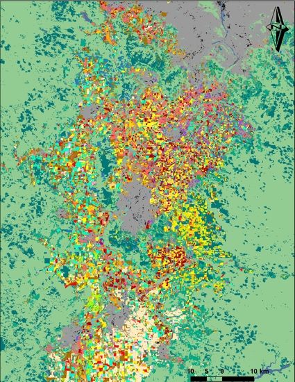
Figure 1.
Digital terrain model and the hydrography of the Willamette Valley and surrounding areas (source: National Hydrography Dataset and Oregon USA).
Figure 1.
Digital terrain model and the hydrography of the Willamette Valley and surrounding areas (source: National Hydrography Dataset and Oregon USA).


Table 1.
Western Oregon 2014 forest and urban development area as previously published [3].
Table 1.
Western Oregon 2014 forest and urban development area as previously published [3].
| Class Areas | Classification Accuracy (%) | ||||
|---|---|---|---|---|---|
| Class | Superclass | Description | (km2) | Producer’s | User’s |
| 11 | 3 | poplars | 0.4 | 76.9 | 99.4 |
| 20 | 3 | Christmas trees | 191.9 | 84.9 | 90.1 |
| 31 | 4 | development | 24.4 | 54.6 | 78.3 |
| 33 | 3 | reforestation | 926.1 | 96.5 | 60.9 |
| 34 | 3 | trees other than poplars | 2.8 | 55.7 | 48.9 |
| 37 | 3 | oak trees | 106.4 | 88.3 | 76.3 |
| 39 | 3 | shrubs, wildlife refuge | 3.5 | 82.6 | 99.8 |
| 45 | 3 | NLCD 11 open water | 176.2 | 98.5 | 100.0 |
| 46 | 3 | NLCD 90 woody wetlands | 164.9 | 95.3 | 97.1 |
| 47 | 3 | NLCD 95 herbaceous wetlands | 18.0 | 86.0 | 96.1 |
| 48 | 4 | NLCD 21 developed open space | 1402.8 | 54.0 | 46.3 |
| 49 | 4 | NLCD 22 developed low intensity | 593.7 | 43.7 | 75.6 |
| 50 | 4 | NLCD 23 developed medium intensity | 663.7 | 81.2 | 52.6 |
| 51 | 3 | NLCD 41 deciduous forest | 1645.5 | 70.7 | 53.8 |
| 52 | 3 | NLCD 43 evergreen forest | 7123.7 | 78.1 | 88.4 |
| 53 | 3 | NLCD 44 mixed forest | 4479.0 | 70.6 | 67.7 |
| 54 | 3 | NLCD 53 scrub/shrub | 1571.7 | 46.2 | 78.7 |
| 57 | 4 | NLCD 24 developed high intensity | 197.5 | 55.0 | 71.8 |
Table 2.
Single year and two-year-long sequential land-use classification categories.
| Class | Superclass | Description | Subsequent Year Options in Two-Year-Long SEQUENCES Sequences (137 Total Cases) |
|---|---|---|---|
| 1 | 1 | bare ground in fall | 1,3,13,14,15,16,27,28,35,55 |
| 2 +12 +44 | 1 | full straw Annual ryegrass +fall plant Annual ryegrass +Annual ryegrass pasture | 1,2,3,13,14,15,16,17,30 |
| 3 +41 | 1 | spring plant new grass Seed +spring plant GS, peas | 1,3,4,5,6,13,15,19 |
| 4 | 2 | established PR | 1,3,4,13,15,16,17,27,30,35,43,55 |
| 5 | 2 | established OG | 5,3 |
| 6 | 2 | established TF | 1,3,6,14,15,16,30,35,43 |
| 7 +10 | 2 | pasture +haycrop | 7,13,16 |
| 8 | 2 | established clover | 3,8,13,14,16,40 |
| 9 | 2 | established mint | 9 |
| 13 | 1 | fall plant PR | 1,3,4,13,16,30,35 |
| 14 | 1 | fall plant TF | 3,6 |
| 15 | 1 | fall plant clover | 8,13,35 |
| 16 | 1 | wheat or other cereals | 1,2,3,7,13,14,15,16,17,28,35,43 |
| 17 | 1 | meadowfoam | 13,16 |
| 18 | 2 | established bentgrass | 1,13,18 |
| 19 | 2 | established fine fescue | 13,16,19,30 |
| 21 | 2 | wild rice | 21 |
| 22 | 2 | wetland restoration | 22 |
| 23 | 2 | established alfalfa | 13,23 |
| 24 | 2 | established blueberries | 24 |
| 25 | 2 | filberts | 25 |
| 26 | 2 | caneberries | 26 |
| 27 | 1 | corn or sorghum | 1,13,16,27 |
| 28 | 2 | nursery crops | 1,3,13,16,28,35 |
| 29 | 2 | orchards (apple, cherry) | 29 |
| 30 | 1 | fallow | 1,3,13,16 |
| 32 | 2 | vineyards | 32 |
| 35 | 1 | beans summer annuals | 1,3,13,16,27,35 |
| 36 | 1 | flowers | 36,1 |
| 38 | 2 | established hops | 38 |
| 40 | 1 | NT (no till) fall plant TF | 18 |
| 42 | 1 | new planting filberts, hops, blueberries | 24,38,25 |
| 43 | 1 | new planting alfalfa | 13,16,23 |
| 55 | 1 | radish, brassicas | 1,13,16 |
| 56 | 2 | strawberries | 56 |
Table 3.
Overall classification accuracy by year for training and validation datasets of 35 agricultural land-use classes prior to and following 230 cycles optimizing year-to-year consistency.
Table 3.
Overall classification accuracy by year for training and validation datasets of 35 agricultural land-use classes prior to and following 230 cycles optimizing year-to-year consistency.
| Initial Classification | After 230 Cycles of Optimization | |||
|---|---|---|---|---|
| Year | Training Set | Validation Set | Training Set | Validation Set |
| (% Accuracy) | ||||
| 2004 | 48.4 | 48.1 | 55.2 | 55.1 |
| 2005 | 51.4 | 51.0 | 56.8 | 56.3 |
| 2006 | 55.6 | 55.5 | 62.0 | 61.7 |
| 2007 | 51.3 | 51.2 | 56.4 | 56.1 |
| 2008 | 55.5 | 55.4 | 65.4 | 65.2 |
| 2009 | 58.7 | 58.4 | 64.3 | 64.0 |
| 2010 | 40.2 | 40.2 | 56.6 | 56.3 |
| 2011 | 32.8 | 32.9 | 56.3 | 56.0 |
| 2012 | 53.3 | 53.2 | 60.6 | 60.2 |
| 2013 | 66.2 | 65.8 | 65.3 | 65.0 |
| 2014 | 92.1 | 91.7 | 81.9 | 81.5 |
| 2015 | 94.8 | 94.5 | 88.1 | 87.7 |
| 2016 | 96.3 | 96.1 | 80.8 | 80.6 |
| 2017 | 96.3 | 96.0 | 97.4 | 97.1 |
Table 4.
Overall classification kappa by year for training and validation datasets of 35 agricultural land-use classes prior to and following 230 cycles optimizing year-to-year consistency.
Table 4.
Overall classification kappa by year for training and validation datasets of 35 agricultural land-use classes prior to and following 230 cycles optimizing year-to-year consistency.
| Initial Classification | After 230 Cycles of Optimization | |||
|---|---|---|---|---|
| Year | Training Set | Validation Set | Training Set | Validation Set |
| (Kappa) | ||||
| 2004 | 0.476 | 0.473 | 0.545 | 0.543 |
| 2005 | 0.509 | 0.505 | 0.563 | 0.558 |
| 2006 | 0.552 | 0.551 | 0.617 | 0.614 |
| 2007 | 0.508 | 0.506 | 0.559 | 0.556 |
| 2008 | 0.551 | 0.550 | 0.651 | 0.650 |
| 2009 | 0.584 | 0.581 | 0.641 | 0.638 |
| 2010 | 0.395 | 0.394 | 0.560 | 0.558 |
| 2011 | 0.320 | 0.322 | 0.559 | 0.555 |
| 2012 | 0.527 | 0.526 | 0.602 | 0.597 |
| 2013 | 0.660 | 0.656 | 0.651 | 0.648 |
| 2014 | 0.921 | 0.917 | 0.818 | 0.815 |
| 2015 | 0.948 | 0.945 | 0.881 | 0.877 |
| 2016 | 0.963 | 0.961 | 0.808 | 0.806 |
| 2017 | 0.963 | 0.960 | 0.974 | 0.971 |
Table 5.
Overall classification accuracy by year-to-year sequence of 137 two-year-long-transitions for training and validation datasets prior to and following 230 cycles optimizing year-to-year consistency.
Table 5.
Overall classification accuracy by year-to-year sequence of 137 two-year-long-transitions for training and validation datasets prior to and following 230 cycles optimizing year-to-year consistency.
| Initial Classification | After 230 Cycles of Optimization | |||
|---|---|---|---|---|
| Year | Training Set | Validation Set | Training Set | Validation Set |
| (% Accuracy) | ||||
| 2004–2005 | 43.3 | 42.3 | 47.1 | 46.7 |
| 2005–2006 | 74.7 | 73.4 | 49.4 | 48.6 |
| 2006–2007 | 72.8 | 71.6 | 48.3 | 48.0 |
| 2007–2008 | 73.8 | 72.5 | 55.3 | 54.7 |
| 2008–2009 | 73.4 | 71.9 | 57.6 | 57.1 |
| 2009–2020 | 70.6 | 69.1 | 49.8 | 49.5 |
| 2010–2011 | 68.6 | 67.7 | 49.5 | 49.3 |
| 2011–2012 | 67.4 | 66.4 | 47.2 | 46.7 |
| 2012–2013 | 75.7 | 74.1 | 50.7 | 50.2 |
| 2013–2014 | 96.6 | 96.1 | 78.5 | 78.1 |
| 2014–2015 | 98.2 | 97.6 | 84.9 | 84.5 |
| 2015–2016 | 99.1 | 98.5 | 86.3 | 86.0 |
| 2016–2017 | 98.6 | 98.0 | 94.2 | 94.1 |
Table 6.
Overall classification kappa by year-to-year sequence of 137 two-year-long transitions for training and validation datasets prior to and following 230 cycles optimizing year-to-year consistency.
Table 6.
Overall classification kappa by year-to-year sequence of 137 two-year-long transitions for training and validation datasets prior to and following 230 cycles optimizing year-to-year consistency.
| Initial Classification | After 230 Cycles of Optimization | |||
|---|---|---|---|---|
| Year | Training Set | Validation Set | Training Set | Validation Set |
| (Kappa) | ||||
| 2004–2005 | 0.432 | 0.423 | 0.471 | 0.466 |
| 2005–2006 | 0.747 | 0.734 | 0.493 | 0.486 |
| 2006–2007 | 0.728 | 0.715 | 0.482 | 0.479 |
| 2007–2008 | 0.738 | 0.725 | 0.553 | 0.547 |
| 2008–2009 | 0.733 | 0.719 | 0.576 | 0.571 |
| 2009–2020 | 0.705 | 0.691 | 0.498 | 0.495 |
| 2010–2011 | 0.685 | 0.677 | 0.494 | 0.493 |
| 2011–2012 | 0.674 | 0.664 | 0.471 | 0.467 |
| 2012–2013 | 0.757 | 0.741 | 0.506 | 0.501 |
| 2013–2014 | 0.966 | 0.961 | 0.785 | 0.781 |
| 2014–2015 | 0.982 | 0.976 | 0.849 | 0.845 |
| 2015–2016 | 0.991 | 0.985 | 0.863 | 0.860 |
| 2016–2017 | 0.986 | 0.980 | 0.942 | 0.941 |
Table 7.
Land-use classification category area and accuracy as the 14-year average from 2004 to 2017.
Table 7.
Land-use classification category area and accuracy as the 14-year average from 2004 to 2017.
| Class | Superclass | Description | Class Areas | Classification Accuracy (%) | |
|---|---|---|---|---|---|
| (km2) | Producer’s | User’s | |||
| 1 | 1 | bare ground in fall | 398.3 | 55.8 | 56.5 |
| 2 +12 +44 | 1 | full straw Annual ryegrass +fall plant Annual ryegrass +Annual ryegrass pasture | 646.3 | 70.3 | 59.1 |
| 3 +41 | 1 | spring plant new grass seed +spring plant GS, peas | 121.2 | 74.0 | 74.5 |
| 4 | 2 | established PR | 426.3 | 70.2 | 63.6 |
| 5 | 2 | established OG | 78.6 | 73.4 | 71.7 |
| 6 | 2 | established TF | 489.4 | 67.9 | 58.5 |
| 7 +10 | 2 | pasture +haycrop | 1191.0 | 65.7 | 32.0 |
| 8 | 2 | established clover | 37.6 | 76.6 | 82.9 |
| 9 | 2 | established mint | 7.2 | 61.7 | 93.2 |
| 13 | 1 | fall plant PR | 147.6 | 65.9 | 74.8 |
| 14 | 1 | fall plant TF | 17.9 | 64.0 | 82.5 |
| 15 | 1 | fall plant clover | 27.4 | 54.8 | 85.9 |
| 16 | 1 | wheat or other cereals | 407.1 | 68.7 | 67.4 |
| 17 | 1 | meadowfoam | 5.8 | 43.1 | 92.0 |
| 18 | 2 | established bentgrass | 10.8 | 46.3 | 84.4 |
| 19 | 2 | established fine fescue | 78.1 | 69.4 | 71.2 |
| 21 | 2 | wild rice | 23.3 | 76.6 | 80.9 |
| 22 | 2 | wetland restoration | 4.0 | 70.3 | 97.0 |
| 23 | 2 | established alfalfa | 1.6 | 55.8 | 95.4 |
| 24 | 2 | established blueberries | 24.0 | 84.4 | 74.4 |
| 25 | 2 | filberts | 361.5 | 87.3 | 36.3 |
| 26 | 2 | caneberries | 77.2 | 54.1 | 47.9 |
| 27 | 1 | corn or sorghum | 48.6 | 53.9 | 60.2 |
| 28 | 2 | nursery crops | 624.5 | 60.3 | 33.1 |
| 29 | 2 | orchards (apple, cherry) | 55.1 | 56.8 | 69.9 |
| 30 | 1 | fallow | 26.1 | 49.3 | 71.4 |
| 32 | 2 | vineyards | 115.4 | 76.4 | 62.3 |
| 35 | 1 | beans summer annuals | 43.9 | 53.3 | 65.2 |
| 36 | 1 | flowers | 2.3 | 30.5 | 91.7 |
| 38 | 2 | established hops | 18.6 | 75.7 | 69.0 |
| 40 | 1 | NT (no till) fall plant TF | 0.2 | 10.8 | 96.9 |
| 42 | 1 | new planting filberts, hops, blueberries | 1.8 | 36.2 | 86.9 |
| 43 | 1 | new planting alfalfa | 12.2 | 50.8 | 81.3 |
| 55 | 1 | radish, brassicas | 4.4 | 37.7 | 90.0 |
| 56 | 2 | strawberries | 0.1 | 49.3 | 99.7 |
Table 8.
Producer’s accuracy relative to ground-truth training datasets by classification category and year after 230 cycles of year-to-year optimization.
Table 8.
Producer’s accuracy relative to ground-truth training datasets by classification category and year after 230 cycles of year-to-year optimization.
| Producer’s Accuracy by Year and Class from Ground-Truth Training Datasets for Final Optimized Classifications of 35 Agricultural Land-Uses (%) | ||||||||||||||
|---|---|---|---|---|---|---|---|---|---|---|---|---|---|---|
| Class | 2004 | 2005 | 2006 | 2007 | 2008 | 2009 | 2010 | 2011 | 2012 | 2013 | 2014 | 2015 | 2016 | Class |
| 1 | 43.5 | 60.8 | 62.0 | 48.4 | 61.3 | 53.6 | 47.1 | 50.9 | 57.3 | 49.2 | 63.1 | 84.9 | 79.9 | 98.2 |
| 2 * | 63.1 | 68.9 | 70.2 | 55.7 | 69.1 | 64.4 | 64.8 | 52.3 | 64.8 | 86.4 | 89.0 | 96.6 | 95.8 | 97.8 |
| 3 * | 81.4 | 72.2 | 60.5 | 70.1 | 74.9 | 70.1 | 76.8 | 77.0 | 70.7 | 94.7 | 95.7 | 96.2 | ||
| 4 | 57.4 | 50.2 | 73.5 | 69.6 | 71.9 | 71.8 | 69.5 | 52.1 | 61.0 | 77.7 | 92.5 | 84.1 | 95.2 | 93.8 |
| 5 | 77.5 | 63.8 | 72.7 | 64.2 | 83.6 | 66.2 | 78.1 | 59.5 | 56.0 | 67.7 | 86.3 | 94.4 | 84.0 | 97.5 |
| 6 | 36.3 | 31.0 | 58.7 | 72.9 | 67.7 | 78.2 | 69.2 | 53.5 | 77.5 | 78.8 | 92.7 | 93.1 | 92.4 | 95.6 |
| 7 * | 63.0 | 56.1 | 51.1 | 55.7 | 57.6 | 63.6 | 65.0 | 67.1 | 64.7 | 79.0 | 94.3 | 97.0 | 96.2 | 97.9 |
| 8 | 57.9 | 52.8 | 85.8 | 81.2 | 75.1 | 85.5 | 80.1 | 80.7 | 82.8 | 71.1 | 92.9 | 78.9 | 56.1 | 98.2 |
| 9 | 65.1 | 64.4 | 76.6 | 46.0 | 38.4 | 38.9 | 84.4 | 48.5 | 86.7 | 61.0 | 53.1 | 89.5 | ||
| 13 | 58.5 | 61.9 | 55.1 | 67.7 | 73.5 | 64.1 | 56.1 | 65.0 | 66.2 | 83.5 | 92.0 | 84.4 | 98.7 | |
| 14 | 59.7 | 85.3 | 67.1 | 54.2 | 68.1 | 71.1 | 43.8 | 55.7 | 63.1 | 67.6 | 99.9 | 81.5 | ||
| 15 | 79.5 | 54.5 | 39.2 | 63.0 | 50.6 | 45.2 | 46.6 | 43.5 | 44.8 | 51.5 | 81.7 | 63.9 | 96.9 | |
| 16 | 46.9 | 58.1 | 69.6 | 60.0 | 74.6 | 68.1 | 45.9 | 70.7 | 63.3 | 72.1 | 89.3 | 95.2 | 89.8 | 96.8 |
| 17 | 33.8 | 34.3 | 34.3 | 53.7 | 45.1 | 25.0 | 43.7 | 47.3 | 9.9 | 45.9 | 86.4 | 0.0 | 98.1 | |
| 18 | 52.0 | 31.6 | 21.3 | 33.2 | 51.5 | 51.3 | 77.5 | 65.4 | 47.6 | 49.5 | 39.3 | 45.9 | 99.8 | 99.8 |
| 19 | 53.1 | 72.4 | 72.5 | 52.8 | 65.5 | 63.9 | 78.4 | 59.9 | 62.9 | 75.5 | 90.8 | 80.1 | 93.0 | 96.7 |
| 21 | 97.0 | 97.0 | 100.0 | 98.6 | 98.5 | 76.7 | 46.4 | 28.7 | 41.2 | 71.3 | 99.2 | 99.3 | 99.2 | 99.2 |
| 22 | 39.0 | 38.8 | 39.1 | 35.7 | 39.7 | 53.2 | 44.9 | 54.6 | 79.9 | 91.0 | 96.1 | 98.9 | 99.3 | |
| 23 | 71.2 | 40.8 | 50.0 | 80.7 | 86.5 | 72.6 | 22.1 | 47.6 | 70.7 | 99.7 | 76.5 | 75.9 | 95.7 | 100.0 |
| 24 | 89.6 | 90.5 | 97.7 | 97.0 | 94.6 | 86.7 | 75.2 | 54.1 | 70.6 | 81.8 | 95.3 | 93.4 | 98.0 | 97.9 |
| 25 | 87.7 | 86.9 | 89.2 | 89.7 | 87.0 | 78.7 | 79.3 | 75.8 | 80.9 | 89.6 | 80.8 | 93.7 | 95.4 | 96.7 |
| 26 | 37.3 | 44.9 | 46.0 | 42.3 | 38.9 | 36.7 | 27.4 | 36.3 | 51.7 | 77.8 | 90.3 | 95.3 | 92.7 | 96.4 |
| 27 | 48.9 | 89.2 | 90.5 | 73.3 | 57.3 | 37.2 | 59.9 | 53.7 | 48.3 | 88.8 | 64.5 | 17.6 | 100.0 | |
| 28 | 58.3 | 44.3 | 51.8 | 62.3 | 54.4 | 64.9 | 56.3 | 51.4 | 56.5 | 81.8 | 93.3 | 91.8 | 97.0 | 96.9 |
| 29 | 48.0 | 53.3 | 63.3 | 65.0 | 57.9 | 50.8 | 46.5 | 35.5 | 37.6 | 65 | 78.2 | 85.3 | 25.4 | 46.5 |
| 30 | 51.5 | 46.0 | 51.2 | 53.2 | 66.2 | 54.0 | 57.7 | 31.6 | 74.9 | 54.1 | 6.3.0 | 94.7 | ||
| 32 | 49.3 | 45.1 | 56.7 | 70.5 | 74.3 | 78.3 | 77.1 | 73.6 | 71.9 | 86.3 | 95.7 | 96.9 | 99.8 | 99.8 |
| 35 | 80.6 | 60.9 | 53.8 | 37.8 | 68.7 | 56.0 | 90.6 | 81.9 | 29.4 | 36.8 | 67.1 | 44.1 | 99.8 | |
| 36 | 97.6 | 22.7 | 29.6 | 29.5 | 38.3 | 34.1 | 15.9 | 11.3 | 100.0 | 15.3 | 71.8 | 98.0 | 97.8 | |
| 38 | 72.4 | 67.3 | 75.7 | 78.5 | 81.2 | 72.3 | 65.7 | 45.3 | 88.3 | 95.4 | 98.6 | 99.7 | 99.6 | 99.6 |
| 40 | 0.0 | 25.5 | 0.1 | 0.0 | 42.8 | 0.0 | 0.0 | 3.6 | ||||||
| 42 | 0.0 | 1.2 | 14.3 | 0.0 | 50.0 | 6.6 | 0.0 | 68.5 | 78.8 | 0.0 | 90.6 | |||
| 43 | 26.0 | 0.6 | 35.8 | 19.1 | 47.0 | 61.4 | 43.9 | 77.1 | 46.0 | 65.2 | 76.5 | 36.8 | 98.8 | |
| 55 | 96.0 | 33.9 | 36.1 | 64.9 | 2.3 | 63.2 | 39.1 | 9.2 | 20.2 | 24.3 | 41.9 | 35.7 | 9.7 | 98.8 |
| 56 | 95.0 | 98.6 | 98.6 | 36.9 | 89.0 | 98.4 | 4.2 | 77.1 | 11.4 | 72.3 | 0.0 | |||
* Classes 2, 12, and 44 (as pooled class 2), classes 3 and 41 (as pooled class 3), and classes 7 and 10 (as pooled class 7) were merged before initial maximum likelihood classifications for 35-class individual year and 137-class 2-year cropping sequences. Empty cells lacked any ground-truth data for the missing classes in the given year.
Publisher’s Note: MDPI stays neutral with regard to jurisdictional claims in published maps and institutional affiliations. |
© 2021 by the authors. Licensee MDPI, Basel, Switzerland. This article is an open access article distributed under the terms and conditions of the Creative Commons Attribution (CC BY) license (http://creativecommons.org/licenses/by/4.0/).
Share and Cite
MDPI and ACS Style
Strimbu, B.M.; Mueller-Warrant, G.; Trippe, K. Agricultural Crop Change in the Willamette Valley, Oregon, from 2004 to 2017. Data 2021, 6, 17. https://0-doi-org.brum.beds.ac.uk/10.3390/data6020017
AMA Style
Strimbu BM, Mueller-Warrant G, Trippe K. Agricultural Crop Change in the Willamette Valley, Oregon, from 2004 to 2017. Data. 2021; 6(2):17. https://0-doi-org.brum.beds.ac.uk/10.3390/data6020017
Chicago/Turabian StyleStrimbu, Bogdan M., George Mueller-Warrant, and Kristin Trippe. 2021. "Agricultural Crop Change in the Willamette Valley, Oregon, from 2004 to 2017" Data 6, no. 2: 17. https://0-doi-org.brum.beds.ac.uk/10.3390/data6020017