
Explainable Machine Learning for Financial Distress Prediction: Evidence from Vietnam


1
Faculty of Banking, Ho Chi Minh University of Banking, No. 36 Ton That Dam Street, Nguyen Thai Binh Ward, District 1, Ho Chi Minh City 700000, Vietnam
2
Institute for Research Science and Banking Technology, Ho Chi Minh University of Banking, No. 36 Ton That Dam Street, Nguyen Thai Binh Ward, District 1, Ho Chi Minh City 700000, Vietnam
3
Department of Economic Mathematics, Ho Chi Minh University of Banking, No. 36 Ton That Dam Street, Nguyen Thai Binh Ward, District 1, Ho Chi Minh City 700000, Vietnam
*
Author to whom correspondence should be addressed.
Data 2022, 7(11), 160; https://0-doi-org.brum.beds.ac.uk/10.3390/data7110160
Submission received: 13 October 2022
/
Revised: 4 November 2022
/
Accepted: 7 November 2022
/
Published: 14 November 2022
(This article belongs to the Special Issue Second Edition of Data Analysis for Financial Markets)
Abstract
:The past decade has witnessed the rapid development of machine learning applied in economics and finance. Recent evidence suggests that machine learning models have produced superior results to traditional statistical models and have become the driving force for dramatic improvement in the financial industry. However, a much-debated question is whether the prediction results from black box machine learning models can be interpreted. In this study, we compared the predictive power of machine learning algorithms and applied SHAP values to interpret the prediction results on the dataset of listed companies in Vietnam from 2010 to 2021. The results showed that the extreme gradient boosting and random forest models outperformed other models. In addition, based on Shapley values, we also found that long-term debts to equity, enterprise value to revenues, account payable to equity, and diluted EPS had greatly influenced the outputs. In terms of practical contributions, the study helps credit rating companies have a new method for predicting the possibility of default of bond issuers in the market. The study also provides an early warning tool for policymakers about the risks of public companies in order to develop measures to protect retail investors against the risk of bond default.
1. Introduction
Financial distress refers to the situation in which a company fail to meet debt obligations to its creditors at maturity. The prolonged and severe financial distress can eventually lead to bankruptcy. Traditionally, the assessment of the financial distress situation of companies was mainly based on the subjective judgment of experts. However, this expert-based approach exposes many drawbacks, including the results are inconsistent, cannot be validated and are highly dependent on expert competence. Therefore, other approaches have been developed to improve consistency and accuracy.These classification techniques can be categorized into statistical methods and machine learning methods. Statistical methods include univariate analysis [1], multiple discriminant analysis [2], logistic regression [3], and Cox survival model [4]. Statistical models are simple in structure, highly explanatory, and take less time to train. However, statistical models require many strict assumptions unavailable in real life, including linear relationships, homogeneity of variances and independence assumptions. Violation of these assumptions can reduce the predictive power of statistical methods. Then, the development of machine learning algorithms marked a breakthrough in the science of prediction. The application of machine learning models, such as support vector machine [5], decision tree [6], and artificial neural networks [7], have enhanced the predictive power of traditional models. Recently, ensemble models such as random forest [8], adaptive boosting [9], and extreme gradient boosting [10] have become significant drivers of developments in the economy and financial sectors, especially in risk management. Although providing better forecasting results, machine learning methods also have drawbacks, as these models are complex and unable to interpret. Meanwhile, explaining and interpreting become extremely necessary for internal use, such as by managers and programmers, and external stakeholders, such as creditors, shareholders, credit rating agencies, and regulators.
Recently, studies have been conducted to enhance the explainability of the machine learning models, but they mainly focused on P2P loans and the SME loans market. In this study, we aim to apply machine learning and enhance the explainability of forecasting results on the data of listed companies in Vietnam. Our study contributes to two new points to the area of risk forecasting. Firstly, to our best knowledge, this is a pioneering study in applying machine learning to predict financial distress in the dataset of companies in Vietnam. Second, we also found important features that explain the forecast results using the SHAP values. Based on the results, we also gained more valuable information to improve the risk assessment process of debt issuers.
The rest of this study is organized as follows. Section 2 reviews the literature on financial distress prediction, the introduction of explanatory techniques, and highlights the contribution of previous research. Section 3 presents the methodologies and techniques used in this research. Section 4 shows the results of the prediction and interpretation. Section 5 concludes with conclusions and limitations of this study.
2. Literature Review
2.1. Literature Review on Financial Distress Prediction
Default risk prediction models based on statistical techniques were built and developed in the late 1960s. Beaver [1] applied regression models to determine 30 financial ratios that significantly impact the corporate default risk. Later, Altman [2] improved Beaver’s work by developing a multiple discriminant analysis method to predict bankruptcy. He built a Z-score model that employed a discriminant function to classify the observation. However, discriminant model also has some disadvantages, such as (i) assuming a linear relationship between the independent variable and the dependent variable; (ii) the results are difficult to interpret and cannot quantify the level of risk between different groups. In 1980, Ohlson pioneered applied logistic regression models to predict the probability of default of corporates. The advantage of this model is that the outputs are the borrower’s probability of default, but the accuracy of the model is not always high [11].
Because the credit analysis process is similar to pattern recognition problems, machine learning algorithms have been employed to classify borrowers’ creditworthiness [11]. Having less restrictive constraints than Altman and Olson’s model, support vector machines (SVM) have been developed to solve the classification problem. [12]. Chen et al. [13] used the SVM model to predict the bankruptcy risk of German firms. The study proved that the SVM model produced better results than the traditional logit model. Moreover, the authors found that the SVM model can better exploit the nonlinear relationships between coefficients and default risk than traditional models such as discriminant or logit models. Shin et al. [14] also applied SVM to predict bankruptcy for 2320 medium-sized enterprises at the Korea Credit Guarantee Fund from 1996 to 1999. The results showed that SVM brought better predictive results than other models, including artificial neural network (ANN) models.
Zhao et al. [15] conducted a study to build a credit scoring system based on ANN on the German credit data dataset. The results showed that ANN could predict credit scores more accurately than traditional models, with an efficiency of 87%. Geng et al. [16] used machine learning models to predict financial distress for firms listed on the Shanghai and Shenzhen stock exchanges from 2001 to 2008. They found that the ANN model produced better results than decision trees, SVM, and assembled models. Barboza et al. [17] used SVM, bagging, boosting, and random forest methods to predict the bankruptcy of 10,000 companies in the North American market from 1985 to 2013 and compared them with traditional statistical models. The results showed that bagging, boosting, and random forest outperforms the others. Specifically, machine learning models had an average accuracy of about 10% higher than traditional models. In more detail, the random forest model had an accuracy of up to 87%, while the traditional model had an accuracy of 50% to 69%. Chakraborty and Joseph [18] constructed a predictive model of financial distress based on balance sheet items. They found that the random forest model showed better results than 10 percent measured by AUC ROC. Similarly, Fuster et al. [19] studied mortgage defaults in the US and found that a random forest model had more accurate predictive results than the logistic model. Based on recent research by Dubyna et al. [20], the use of technologies in the provision of financial services is extremely important, influencing the transformation of the financial behavior of customers and the business models of financial institutions. In addition, research by Zhavoronok et al. [21] shows that innovation processes affect the financial behavior patterns of households in innovative economies in different meanings and forms.
Previous studies have proved that machine learning models yield better results than traditional statistical models. However, the results are not consistent and depend on the data set used in the study. In addition, machine learning models also have drawbacks such as (i) they do not work well for unbalanced data because they tend to classify many observations into classes with more larger data; (ii) model accuracy increases with a more extensive training dataset, but validation is insufficient to meet a certain rate (iii) selecting hidden later layers is problematic, resulting in a trade-off between computation time and high prediction rate [15].
2.2. Literature Review on Explanation
Interpretability is the ability to explain or present in terms that can be understood by humans [22]. Miller [23] defined explainability as the degree to which people can understand the causes of a decision. Thus, an interpretable system is a system that provides knowledge that helps people understand how it works and can interpret the results of a specific forecast.
Since 2019, studies have focused on the explanatory power of deep learning models in predicting default. Bracke et al. [24] used the gradient tree boosting model to predict default on mortgage loans in the UK. They introduced a new method named quantitative input influence (QII) to evaluate the contribution of the input variables to the target variable by calculating the Shapley values. The authors showed that this method could provide a detailed explanation of the degree of impact of the variables on different customer groups.
Later, some studies used the Shapley values to measure the contribution of variables in the model to the target variable. Babaei et al. [25] applied machine learning to predict default for small and medium enterprises. The authors eliminated variables with low explanatory Sharley values. The results showed that defaults and expected returns of these companies are better forecasted with a smaller amount of input variables from the financial statements. Bussmann et al. [26] applied XGB machine learning, correlation networks, and Shapley computation on a sample of 15,000 SMEs in Southeast Europe. The results showed that forecasting efficiency could be improved by understanding the factors that affect credit risk in the model.
Additionally, some studies used Shapley Additive exPlanations (SHAP) and Local Interpretable Model-Agnostic Explanations (LIME) methods to compare the explanatory power of the variables in the model [27,28]. Ariza-Garzón et al. [29] compared the predictive power of machine learning algorithms (decision trees, random forests, XGBoost) with logistic regression models on personal loans from Lending Club company. Then, they evaluated the contribution of variables in the model through SHAP and LIME methods. The results showed that when applying SHAP to machine learning methods, the explanatory power of these models was improved, even reflecting the nonlinear relationships better than the traditional logistic regression model. A similar study was conducted by Hadji Misheva et al. [30], and the authors also found the same results. They concluded that explanatory results were stable and consistent with the logical explanations in finance. This study applied the SHAP method to interpret machine learning models’ results.
3. Methodology
3.1. Data and Data Processing
In this study, we used data extracted from the financial statements of Vietnamese companies listed on the Ho Chi Minh Stock Exchange, Hanoi Stock Exchange, and UPCOM. Data were collected from 2010 to 2021.
Financial distress companies are identified based on criteria such as negative equity, EBITDA on interest being less than one for two consecutive years, and operational income being negative for three consecutive years. In addition, we also consult the external auditor’s conclusions in the financial statements and filter out companies suspected of not being able to operate continuously. Finally, the selected insolvency companies meet the above criteria and have sufficient financial data during the observation period to conduct the research. Companies will be labeled one if they are in the financial distress group and zero for the others.
Based on the study of Chakraborty and Joseph [18], and Standard & Poor’s evaluation criteria, we used 25 financial ratios as input features for predictive machine learning models (Appendix A). These ratios reflect essential aspects of companies, such as liquidity, financial risk, business risk, and the market factor, that are expected to affect the debt repayment capacity of companies.
The data were preprocessed for missing values and outliers. We also excluded financial, insurance, accounting, and banking companies because of differences in financial statements. The data had 3277 observations, of which 436 companies were in financial distress (13.3%), and 2841 companies were in the group of non-financial distress (86.7%). Because the data were unbalanced, we used SMOTE technique to handle the unbalance data problem. Finally, the data were divided into training and validation sets, with 70% and 30%, respectively.
3.2. Machine Learning Methods to Predict Financial Distress
In this research, we employed statistical methods and machine learning to predict the distress of businesses, including logistic regression, support vector machine, decision tree, random forest, artificial neural network, and extreme gradient boosting. The details of the methods are presented as follows.
3.2.1. Logistic Regression
Logistic regression is a popular statistical technique for forecasting problems where the dependent variable is binary, specifically, the financial distress status in this study. The output of the model is the probability of financial distress , corresponding to the input features . This probability is calculated as Equation (1).
Logistic regression is often used as a benchmark in research to compare with other forecasting methods. The advantage of logistic regression is that the results are easy to interpret and understand for most users. In other words, this is one of the models with high explanatory power, so it is often used in practice at financial institutions.
3.2.2. Support Vector Machine
Support vector machines (SVMs) are based on the idea of defining hyperplanes that decompose observations into high-dimensional feature spaces. Linear SVMs models focus on maximizing the margin between positive and negative hyperplanes. The classification process will take place according to Equation (2).
where b is the bias.
For nonlinear cases, a kernel is used to project features into a high-dimensional space. For example, a traditional Kernel function, a Gaussian radial basis, has the following Equation (3).
The strength of SVM is that it avoids overfitting with small samples and is less sensitive to unbalanced distributions.
3.2.3. Decision Tree
Decision tree algorithms extract information from data to derive decision rules in the form of a tree structure. More specifically, the decision tree algorithm determines the best allocation to optimize each split with maximum purity based on a measure, such as the Gini Index or Entropy Index. The root of a decision tree is called the root node, the most distinguishable attribute. Leaf nodes represent classes, which are the following attributes.
The decision tree model has the advantage that model is intuitive and interpretable. However, the drawback is that this model is more prone to overfitting during the feature domain division or the branching process.
3.2.4. Random Forest
Breiman [8] developed the random forest technique based on the decision tree model. In this method, many decision trees are constructed using subsets of randomly selected features. The sample and feature subsets are randomly selected to ensure the diversity of the classifiers. Then, the random forest is built for several subsets that generate the same number of classification trees. The preferred class is defined by a majority of votes; thus, the results are more precise and, most importantly, avoid model overfitting [8].
3.2.5. Extreme Gradient Boosting (XGB)
Gradient boosting is a machine-learning technique used in regression and classification tasks. It gives a prediction model in the form of an ensemble of weak prediction models, typically decision trees. Extreme gradient boosting constructs decision trees in parallel and incorporates complexity control in the loss function to control overfitting and achieve better performance results. The optimization function to minimize is as follows in Equation (4).
where is a loss function. is a regularization term that penalizes the complexity of the model. The goal is to find the that minimized the function .
3.2.6. Artificial Neural Network
An artificial neural network (also known as a neural network) is a machine learning algorithm designed based on the idea of how an organism’s brain works. The algorithm solves complex problems by mimicking the brain’s structure and the connections between neurons.
An artificial neural network consists of connections between many layers of artificial neurons. Each layer is divided into an input layer, an output layer, and a hidden layer. These artificial neurons simulate the role of human neurons through mathematical models. Each artificial neuron receives an input signal, , consisting of the numbers 0 and 1, then it estimates the weighted sum of the signals it receives according to their weights, . A signal is only transmitted to the next artificial neuron when the sum of the weights of the received signals exceeds a certain threshold. An artificial neuron can be represented as the Equation (5).
Based on historical data, neural network optimization is conducted by determining weights and thresholds for activation.
3.3. Explainability Methods
SHApely Additive exPlanation (SHAP) is applied to meet interpretation requirements. This algorithm aims to build a linear model explaining the feature importance for a given prediction by computing Shapley sampling values. The SHAP values are calculated based on cooperative game theory in order to explain the prediction through the marginal contribution of each feature. The SHAP model can be represented as a linear combination of the binary variables in the following Equation (6).
where is an explanatory model, is the coalition vector, M is the maximum number of features, the ith feature has a contribution () or not . is the SHAP value of the ith feature, representing the contribution of the ith feature and can be calculated according to the following Equation (7).
where N is the set of all features, |S| represents the number of features in feature subset excluding the ith feature. represents the result of the machine learning model f training in feature subset S.
SHAP is an interpretation technique that works very well on structured data with a limited number of features. SHAP can be interpreted at the global level and on a specific data point. At the global level, feature importance is determined by the average absolute values per feature. In this research, TreeSHAP was employed to compute SHAP values and explain the output of the decision tree and XGBoost models. We chose TreeSHAP because it is a fast and exact method to estimate SHAP values for tree models and ensembles of trees [35]. Moreover, although the tree-based methods, e.g., XGBoost and random forest have their permutation feature importance values, the SHAP values have significant differences with such scales. Permutation feature importance is based on the decrease in model performance. SHAP is based on the magnitude of feature attributions.
3.4. Evaluation of Model Performance
To evaluate the model’s performance, we use the following performance metrics.
- Accuracy—The proportion of correct classification in the evaluation data
- Precision—The proportion of true positives among the predicted positives
- Sensitivity (Recall)—The proportion of positives correctly predicted
- —The harmonic mean of precision and recall.
- The ROC plots the true positive rate to the false positive rate.
- Area under the receiver operating curve (AUC)—The receiver operating curve (ROC) measures the model’s classification ability subject to varying decision boundary thresholds. The area under the curve (AUC) aggregates the performance measures given by the ROC curve. AUC also helps to provide criteria for evaluating and comparing models: AUC had to be more than 0.5 for the model to be acceptable, and the close to 1, the stronger its predictive power.
4. Results and Discussions
4.1. Prediction Results
Table 1 presents the hyper-parameter settings and the evaluation of the models on the model performance metrics. According to Abellán and Castellano [36], the accuracy measure may not be accurate because it does not consider that false positives are more important than false negatives. So, precision and recall are better measures of the model performance, which is more sensitive to the imbalanced dataset. This research also uses the balanced F-score (F1 score), the harmonic mean of precision and recall.
XGB and random forest also have higher recall and F1 scores than other models, indicating that both models are good at predicting positive values. In contrast, logistic regression, ANN, and SVM have relatively low sensitivity values, indicating that these models have higher Type I errors. Interestingly, SVM has the highest value (0.9427), showing the ability to predict the positive accuracy of the predicted values.
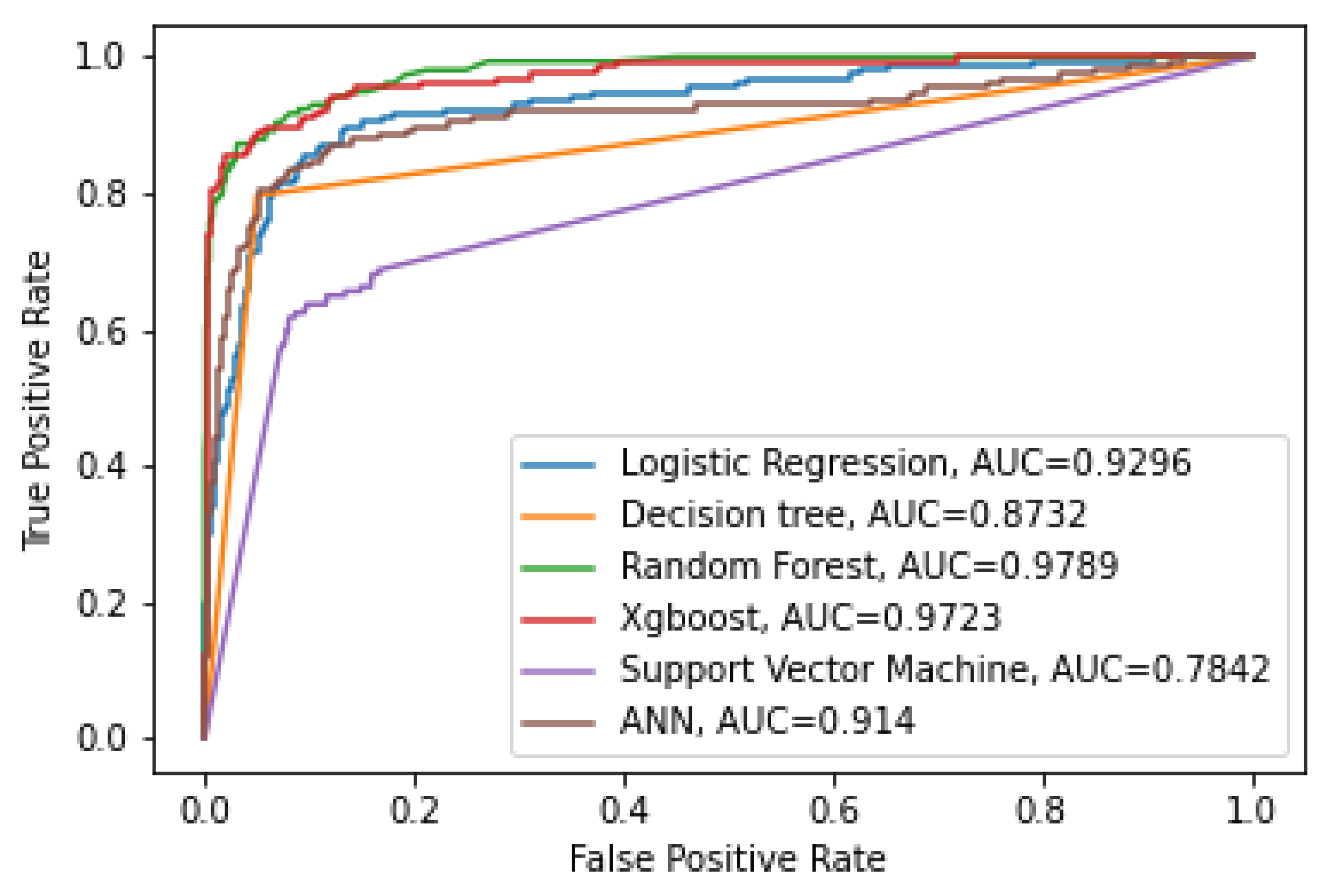
Based on AUC values, it can be seen that random forest has the highest AUC value (0.9788), followed by extreme gradient boosting (0.9702), showing that these two models have better classification ability than other models. These results are similar to the results of Barboza et al. [17]; Chakraborty and Joseph [18]; Fuster et al. [19].
Figure 1 shows that the ROC curve of random forest and XGB closer to the top left corner indicate better performance than other models. It is noted that the ROC does not depend on the class distribution, so it helps evaluate classifiers predicting rare events such as default risk or financial distress risk.
4.2. Interpretation Results
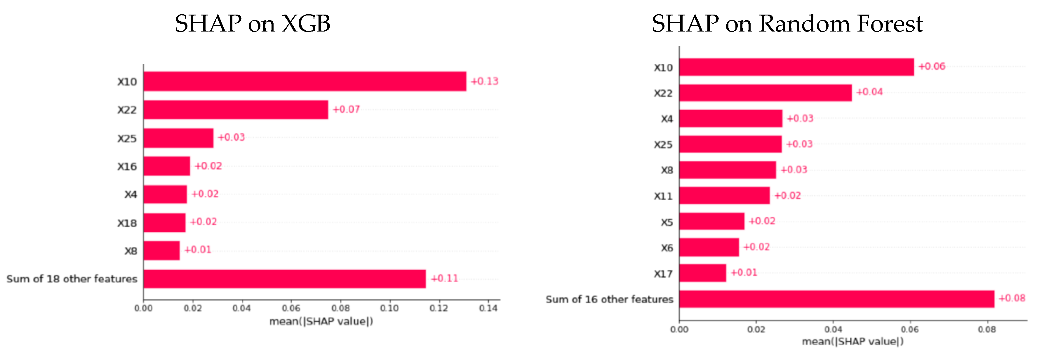
We calculated SHAP values on two models with the best predictive results, random forest and XGBoost. We calculated the average Shapley values across all observations to obtain an “overall” or “global” explanation. This technique was used in the research of Kim and Shin [5] and Bussmann et al. [26].
Figure 2 shows that four of the five important features are the same between the two models. They are long-term debts to equity (X4), account payable to equity (X10), enterprise value to revenues (X22), and diluted EPS (X25). Thus, the important features determined based on Shapley values are relatively stable between XGB and random forest models.
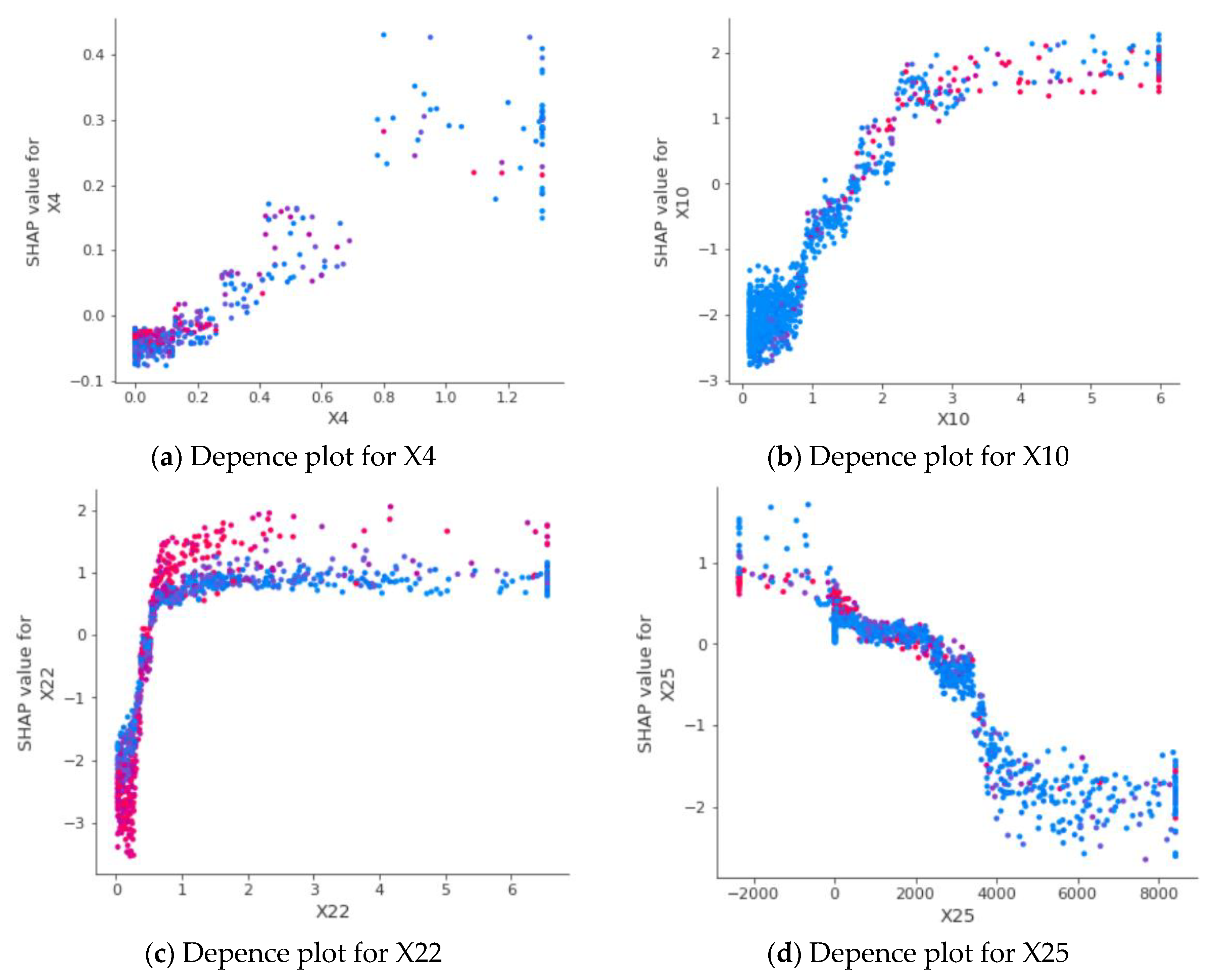
Figure 3a illustrates the influence of long-term debts to equity (X4) on the prediction results. X4 reflects the leverage risk of the company in the long term. If the leverage is high, the company is under tremendous pressure to repay debts and is prone to liquidity risk when the economy is in recession. Figure 3a shows the positive relationship between the X4 and the SHAP values. When the X4 increases, the SHAP values increases, indicating that the probability of financial distress also increases. This phenomenon is in line with the knowledge of financial experts.
Figure 3b displays the dependence plot for account payable to equity (X10). X10 reflects the default risk in the short term. If X10 is high, the company is under pressure to pay short-term debt obligations, which may lead to liquidity risk. When X10 is under 2.5, the SHAP values increase, implying that the likelihood of financial distress increases. However, when the X10 is over 2.5, the SHAP values tend to be stable. This is an interesting phenomenon from observable data, different from experts’ expectations.
Figure 3c shows the influence of enterprise value on revenues (X22) on the prediction results. This ratio measures how much it would cost to purchase a company’s value relative to its revenues. If EV/R increases, the company is overvalued. When the value of X22 is close to 0, the variation of the SHAP value is high. As X22 increases, the SHAP value also gradually increases. However, after X22 is greater than 0.6, the SHAP values tend to be flat. Thus, increasing of X22 will influence SHAP values when X22 is low, but this effect will decrease when X22 is high.
Diluted EPS considers what would happen if dilutive securities were exercised. Figure 3d exhibits the dependent plot for diluted EPS (X25). It can be seen in Figure 3d that there exists a negative relationship between X25 and SHAP values. When X25 increases, SHAP values tend to decrease, reducing the probability of financial distress. However, SHAP values have fluctuated when X25 is less than 0 and greater than 4000.
5. Conclusions
In this study, we employed machine learning models to predict financial distress in listed companies in Vietnam from 2010 to 2021. The results showed that XGB and random forest were two models with higher recall, F1 scores and AUC than other models. In addition, we also used SHAP values to analyze the impacts of each feature on the forecast results. Features such as long-term debts to equity (X4), account payable to equity (X10), enterprise value to revenues (X22), and diluted EPS (X25) showed an significant impact on forecast results and were generally in accordance with the knowledge from experts.
Based on this study, managers, policymakers, and credit rating agencies have equipped tools to understand and interpret results from complex machine learning models. This research has shed light on using XAI to make decisions in economics and finance.
The study also has some limitations, such as low sample size, especially low proportion in financial distress companies. We hope the following studies can expand the sample size by researching countries with similar characteristics. Moreover, the research sample can be expanded to other fields, such as consumer lending or P2P lending.
In addition, the features used in this study are financial indicators, which are based on the assumption that information about companies is reflected in the financial position. However, this assumption is unrealistic in Vietnam, whose financial market is inefficient. We hope that the following studies can add more behavioral features, such as ownership structure, number of independent BOD members, industry, and diversity of business lines.
Author Contributions
Conceived the idea, wrote the Introduction, D.T.N.; wrote literature review, H.A.L.; wrote methodology, results and discussions, conclusion, K.L.T.; revised the manuscript, T.H.N. All authors have read and agreed to the published version of the manuscript.
Funding
The study was supported by The Youth Incubator for Science and Technology Program, managed by the Youth Development Science and Technology Center—Ho Chi Minh Communist Youth Union and Department of Science and Technology of Ho Chi Minh City, the contract number is “14/2021/ HĐ-KHCNT-VU”.
Institutional Review Board Statement
Not applicable.
Informed Consent Statement
Not applicable.
Data Availability Statement
The data for this study can be found on our GitHub page: https://github.com/anhle32/Explainable-Machine-Learning-.git (accessed on 12 October 2022).
Conflicts of Interest
The authors declare no conflict of interest.
Appendix A

Table A1.
Summary of Variables.
| Symbol | Input Features | Category |
|---|---|---|
| X1 | Cash Ratio | Liquidity risk |
| X2 | Quick Ratio | Liquidity risk |
| X3 | Current Ratio | Liquidity risk |
| X4 | Long term Debts to Equity | Financial risk |
| X5 | Long term Debts to Total Assets | Financial risk |
| X6 | Total Liabilities to Equity | Financial risk |
| X7 | Total Liabilities to Total Assets | Financial risk |
| X8 | Short term Debt to Equity | Financial risk |
| X9 | Short term Debt to Total Assets | Financial risk |
| X10 | Account Payable to Equity | Business Risk |
| X11 | Account Payable to Total Assets | Business Risk |
| X12 | Total Assets to Total Liabilities | Business Risk |
| X13 | EBITDA to Short term Debt and Interest | Business Risk |
| X14 | Price to Earning | Market factor |
| X15 | Diluted Price to Earning | Market factor |
| X16 | Price to Book Value | Market factor |
| X17 | Price to Sales | Market factor |
| X18 | Price to Tagible Book Value | Market factor |
| X19 | Market Capital | Market factor |
| X20 | Price to Cashflow | Market factor |
| X21 | Enterprise Value | Valuation |
| X22 | Enterprise Value to Revenues | Valuation |
| X23 | Enterprise Value to EBITDA | Valuation |
| X24 | Enterprise Value to EBIT | Valuation |
| X25 | Diluted EPS | Valuation |
References
- Beaver, W.H. Financial Ratios as Predictors of Failure. J. Account. Res. 1966, 71–111. [Google Scholar] [CrossRef]
- Altman, E.I. Financial Ratios, Discriminant Analysis and the Prediction of Corporate Bankruptcy. J. Financ. 1968, 23, 589–609. [Google Scholar] [CrossRef]
- Ohlson, J.A. Financial Ratios and the Probabilistic Prediction of Bankruptcy. J. Account. Res. 1980, 18, 109–131. [Google Scholar] [CrossRef] [Green Version]
- Cox, D.R. Regression Models and Life-tables. J. R. Stat. Soc. Ser. B (Methodol.) 1972, 34, 187–202. [Google Scholar] [CrossRef]
- Kim, D.; Shin, S. The Economic Explainability of Machine Learning and Standard Econometric Models-an Application to the US Mortgage Default Risk. Int. J. Strateg. Prop. Manag. 2021, 25, 396–412. [Google Scholar] [CrossRef]
- Olson, D.L.; Delen, D.; Meng, Y. Comparative Analysis of Data Mining Methods for Bankruptcy Prediction. Decis. Support Syst. 2012, 52, 464–473. [Google Scholar] [CrossRef]
- Chen, H.-J.; Huang, S.Y.; Lin, C.-S. Alternative Diagnosis of Corporate Bankruptcy: A Neuro Fuzzy Approach. Expert Syst. Appl. 2009, 36, 7710–7720. [Google Scholar] [CrossRef]
- Breiman, L. Random Forests. Mach. Learn. 2001, 45, 5–32. [Google Scholar] [CrossRef] [Green Version]
- Freund, Y.; Schapire, R.; Abe, N. A Short Introduction to Boosting. J. -Jpn. Soc. Artif. Intell. 1999, 14, 1612. [Google Scholar]
- Chen, T.; He, T.; Benesty, M.; Khotilovich, V.; Tang, Y.; Cho, H.; Chen, K. Xgboost: Extreme Gradient Boosting. R Package Version 0.4-2 2015, 1, 1–4. [Google Scholar]
- Kruppa, J.; Schwarz, A.; Arminger, G.; Ziegler, A. Consumer Credit Risk: Individual Probability Estimates Using Machine Learning. Expert Syst. Appl. 2013, 40, 5125–5131. [Google Scholar] [CrossRef]
- Vapnik, V. The Nature of Statistical Learning Theory; Springer Science & Business Media: Berlin/Heidelberg, Germany, 1999; ISBN 0-387-98780-0. [Google Scholar]
- Chen, S.; Härdle, W.K.; Moro, R.A. Modeling Default Risk with Support Vector Machines. Quant. Financ. 2011, 11, 135–154. [Google Scholar] [CrossRef]
- Shin, K.-S.; Lee, T.S.; Kim, H. An Application of Support Vector Machines in Bankruptcy Prediction Model. Expert Syst. Appl. 2005, 28, 127–135. [Google Scholar] [CrossRef]
- Zhao, Z.; Xu, S.; Kang, B.H.; Kabir, M.M.J.; Liu, Y.; Wasinger, R. Investigation and Improvement of Multi-Layer Perceptron Neural Networks for Credit Scoring. Expert Syst. Appl. 2015, 42, 3508–3516. [Google Scholar] [CrossRef]
- Geng, R.; Bose, I.; Chen, X. Prediction of Financial Distress: An Empirical Study of Listed Chinese Companies Using Data Mining. Eur. J. Oper. Res. 2015, 241, 236–247. [Google Scholar] [CrossRef]
- Barboza, F.; Kimura, H.; Altman, E. Machine Learning Models and Bankruptcy Prediction. Expert Syst. Appl. 2017, 83, 405–417. [Google Scholar] [CrossRef]
- Chakraborty, C.; Joseph, A. Machine Learning at Central Banks; SSRN: Amsterdam, The Netherlands, 2017. [Google Scholar]
- Fuster, A.; Goldsmith-Pinkham, P.; Ramadorai, T.; Walther, A. Predictably Unequal? The Effects of Machine Learning on Credit Markets. J. Financ. 2022, 77, 5–47. [Google Scholar] [CrossRef]
- Dubyna, M.; Popelo, O.; Kholiavko, N.; Zhavoronok, A.; Fedyshyn, M.; Yakushko, I. Mapping the Literature on Financial Behavior: A Bibliometric Analysis Using the VOSviewer Program. WSEAS Trans. Bus. Econ. 2022, 19, 231–246. [Google Scholar] [CrossRef]
- Zhavoronok, A..; Popelo, O.; Shchur, R.; Ostrovska, N.; Kordzaia, N. The Role of Digital Technologies in the Transformation of Regional Models of Households’ Financial Behavior in the Conditions of the National Innovative Economy Development. Ingénierie Des Systèmes D’Inf. 2022, 27, 613–620. [Google Scholar] [CrossRef]
- Doshi-Velez, F.; Kim, B. Towards a Rigorous Science of Interpretable Machine Learning. arXiv 2017, arXiv:1702.08608. [Google Scholar]
- Miller, T. Explanation in Artificial Intelligence: Insights from the Social Sciences. Artif. Intell. 2019, 267, 1–38. [Google Scholar] [CrossRef]
- Bracke, P.; Datta, A.; Jung, C.; Sen, S. Machine Learning Explainability in Finance: An Application to Default Risk Analysis; SSRN: Amsterdam, The Netherlands, 2019. [Google Scholar]
- Babaei, G.; Giudici, P.; Raffinetti, E. Explainable Fintech Lending; SSRN: Amsterdam, The Netherlands, 2021. [Google Scholar]
- Bussmann, N.; Giudici, P.; Marinelli, D.; Papenbrock, J. Explainable Machine Learning in Credit Risk Management. Comput. Econ. 2021, 57, 203–216. [Google Scholar] [CrossRef]
- Lundberg, S.M.; Lee, S.-I. A unified approach to interpreting model predictions. In Proceedings of the 31st International Conference on Neural Information Processing Systems, Long Beach, CA, USA, 4 December 2017; pp. 4768–4777. [Google Scholar]
- Ribeiro, M.T.; Singh, S.; Guestrin, C. “Why Should I Trust You?” Explaining the Predictions of Any Classifier. arXiv 2016, arXiv:1602.04938. [Google Scholar]
- Ariza-Garzón, M.J.; Arroyo, J.; Caparrini, A.; Segovia-Vargas, M.-J. Explainability of a Machine Learning Granting Scoring Model in Peer-to-Peer Lending. IEEE Access 2020, 8, 64873–64890. [Google Scholar] [CrossRef]
- Hadji Misheva, B.; Hirsa, A.; Osterrieder, J.; Kulkarni, O.; Fung Lin, S. Explainable AI in Credit Risk Management. Credit. Risk Manag. 2021. [Google Scholar] [CrossRef]
- Harris, C.R.; Millman, K.J.; Van Der Walt, S.J.; Gommers, R.; Virtanen, P.; Cournapeau, D.; Wieser, E.; Taylor, J.; Berg, S.; Smith, N.J. Array Programming with NumPy. Nature 2020, 585, 357–362. [Google Scholar] [CrossRef]
- McKinney, W. Data Structures for Statistical Computing in Python. In Proceedings of the 9th Python in Science Conference, Austin, TX, USA, 28 June–3 July 2010; pp. 51–56. [Google Scholar]
- Pedregosa, F.; Varoquaux, G.; Gramfort, A.; Michel, V.; Thirion, B.; Grisel, O.; Blondel, M.; Prettenhofer, P.; Weiss, R.; Dubourg, V. Scikit-Learn: Machine Learning in Python. J. Mach. Learn. Res. 2011, 12, 2825–2830. [Google Scholar]
- Waskom, M.; Botvinnik, O.; O’Kane, D.; Hobson, P.; Lukauskas, S.; Gemperline, D.C.; Augspurger, T.; Halchenko, Y.; Cole, J.B.; Warmenhoven, J. Mwaskom/Seaborn: V0. 8.1 (September 2017). Zenodo 2017. [Google Scholar] [CrossRef]
- Lundberg, S.M.; Erion, G.; Chen, H.; DeGrave, A.; Prutkin, J.M.; Nair, B.; Katz, R.; Himmelfarb, J.; Bansal, N.; Lee, S.-I. From Local Explanations to Global Understanding with Explainable AI for Trees. Nat. Mach. Intell. 2020, 2, 56–67. [Google Scholar] [CrossRef]
- Abellán, J.; Castellano, J.G. A Comparative Study on Base Classifiers in Ensemble Methods for Credit Scoring. Expert Syst. Appl. 2017, 73, 1–10. [Google Scholar] [CrossRef]
Figure 1.
ROC of classifiers. Source: author’s calculation.

Figure 2.
The feature importance of XGB and random forest. Source: author’s calculation.

Figure 3.
The SHAP dependence plot of single feature. Source: author’s calculation.

Table 1.
The performance results of classifiers.
| Algorithms | Hyper-Parameter | AUC | Accuracy | Precision | Recall | F1 Score | |
|---|---|---|---|---|---|---|---|
| 1 | Extreme Gradient Boosting | booster = “gbtree”, n_estimator = 100, max_depth = 1, random_state = 42 | 0.9702 | 0.9566 | 0.8726 | 0.8354 | 0.8536 |
| 2 | Random Forest | max_depth = 14,n_estimators = 100, random_state = 42 | 0.9788 | 0.9529 | 0.8535 | 0.8272 | 0.8401 |
| 3 | Logistic Regression | random_state = 42 | 0.9303 | 0.8623 | 0.8854 | 0.5148 | 0.6511 |
| 4 | Artificial Neural Network | n_hidden = 2, max_iter = 200, activations = relu, Optimizer = adam | 0.9034 | 0.9168 | 0.8025 | 0.6811 | 0.7368 |
| 5 | Decision Trees | Criterion = “gini”, max_depth = 14, random_state = 42 | 0.8848 | 0.9251 | 0.828 | 0.7065 | 0.7625 |
| 6 | Support Vector Machine | Kernel = “rbf”, probability = True, class_weight = “balanced”, random_state = 42 | 0.7889 | 0.8789 | 0.9427 | 0.4022 | 0.5815 |
Source: author’s calculation.
Publisher’s Note: MDPI stays neutral with regard to jurisdictional claims in published maps and institutional affiliations. |
© 2022 by the authors. Licensee MDPI, Basel, Switzerland. This article is an open access article distributed under the terms and conditions of the Creative Commons Attribution (CC BY) license (https://creativecommons.org/licenses/by/4.0/).
Share and Cite
MDPI and ACS Style
Tran, K.L.; Le, H.A.; Nguyen, T.H.; Nguyen, D.T. Explainable Machine Learning for Financial Distress Prediction: Evidence from Vietnam. Data 2022, 7, 160. https://0-doi-org.brum.beds.ac.uk/10.3390/data7110160
AMA Style
Tran KL, Le HA, Nguyen TH, Nguyen DT. Explainable Machine Learning for Financial Distress Prediction: Evidence from Vietnam. Data. 2022; 7(11):160. https://0-doi-org.brum.beds.ac.uk/10.3390/data7110160
Chicago/Turabian StyleTran, Kim Long, Hoang Anh Le, Thanh Hien Nguyen, and Duc Trung Nguyen. 2022. "Explainable Machine Learning for Financial Distress Prediction: Evidence from Vietnam" Data 7, no. 11: 160. https://0-doi-org.brum.beds.ac.uk/10.3390/data7110160