Article

Fundamentals and Applications of Artificial Neural Network Modelling of Continuous Bifidobacteria Monoculture at a Low Flow Rate

1
Department of Information Computer Technology Chemical and Pharmaceutical Engineering, Mendeleev University of Chemical Technology, 125047 Moscow, Russia
2
Department of Chemical and Pharmaceutical Engineering, Mendeleev University of Chemical Technology, 125047 Moscow, Russia
3
Biotechnology Department, Mendeleev University of Chemical Technology, 125047 Moscow, Russia
*
Author to whom correspondence should be addressed.
Submission received: 6 April 2022 / Revised: 1 May 2022 / Accepted: 3 May 2022 / Published: 6 May 2022

Abstract

:
The application of artificial neural networks (ANNs) to mathematical modelling in microbiology and biotechnology has been a promising and convenient tool for over 30 years because ANNs make it possible to predict complex multiparametric dependencies. This article is devoted to the investigation and justification of ANN choice for modelling the growth of a probiotic strain of Bifidobacterium adolescentis in a continuous monoculture, at low flow rates, under different oligofructose (OF) concentrations, as a preliminary study for a predictive model of the behaviour of intestinal microbiota. We considered the possibility and effectiveness of various classes of ANN. Taking into account the specifics of the experimental data, we proposed two-layer perceptrons as a mathematical modelling tool trained on the basis of the error backpropagation algorithm. We proposed and tested the mechanisms for training, testing and tuning the perceptron on the basis of both the standard ratio between the training and test sample volumes and under the condition of limited training data, due to the high cost, duration and the complexity of the experiments. We developed and tested the specific ANN models (class, structure, training settings, weight coefficients) with new data. The validity of the model was confirmed using RMSE, which was from 4.24 to 980% for different concentrations. The results showed the high efficiency of ANNs in general and bilayer perceptrons in particular in solving modelling tasks in microbiology and biotechnology, making it possible to recommend this tool for further wider applications.

1. Introduction

The colonization of the intestine begins at birth [1] and creates the basis for the future microbial community, which is one of the most important elements for maintaining the health of the body through the life course. Similar processes occur in adults after intensive antibiotics [2] or chemotherapy [3], when the microbial population density in the biotope is reduced and pathogens can begin to dominate, causing gastrointestinal disease. Treatment with probiotics and their synbiotic compositions with prebiotic substances is considered one of the effective ways to restore microbiota [4,5]. There are several studies both confirming and refuting their effectiveness in favour of other types of therapy, such as faecal transplantation [6]. Efforts towards understanding the mechanisms of succession are closely related to the study of changes in the microbial community under the influence of such agents. However, the solution of this problem in vivo is rather difficult. Although the use of both functional and mathematical models gives an approximate picture, it can in this case be very informative and useful.
In this paper, we tried to introduce the process of establishing homeostasis (dynamic equilibrium) in a system that simulates the distal large intestine in vitro based on the functional model proposed by Gibson and McFarlane [7,8]. Moreover, we attempted to enforce this simulation with a mathematical model. The studies were carried out with a Bifidobacterium monoculture. As a sole carbohydrate substrate, oligofructose at concentrations from 2 to 15 g L−1 was used. The experimental conditions simulated the succession of the microbial community (introduction of probiotics or pathogens) in the cases considered above. Meanwhile, the growth conditions did not correspond to a chemostat with an “eternally active culture” and they were not close to optimal. This feature, along with the peculiarities of bifidobacterial physiology, lead to the fact that such processes as the growth and death of microbial cells, as well as their agglomeration and deagglomeration, run at different rates. In such cases, the use of classical models of microbial growth is rather difficult since a large number of model parameters need to be determined. One of the promising approaches for modelling and predicting the behaviour of the microbial community in this case is the use of artificial neural networks.
Artificial neural networks (ANNs) are logical-mathematical apparatus based on the principles of the transmission and processing of information signals in the nervous systems of higher living organisms. They are used for solving tasks associated with the mathematical modelling and simulation of complex multifactorial processes [9,10,11]. Their use is of great interest in different fields of science, including microbiology and biotechnology, since they are able to work quite quickly with large amounts of experimental data and find complex interdependencies between the data with the required level of error. Using a trained neural network model, it is possible to predict the behaviour of a process under new conditions and make conclusions based on that result [12,13,14]. Analysis of the modern use of neural networks for modelling biotechnological processes shows that the classical architecture in the form of single-layer and/or multi-layer perceptrons is most often used.
In ref. [15], the application of model-predictive control based on artificial neural networks is considered to optimize riboflavin production. Two different types of ANN were used: a multilayer perceptron for preliminary experiments on the assessment of biomass and product and ZNet for optimization experiments. The ZNet ANN presented an extension of the perceptron model that divides input data into memory cells, the contents of which were weights adjusted during training. The output data was an algebraic sum of weights in all memory cells activated by input accuracy. The multilayer perceptron consisted of 5 input neurons, one hidden layer of 20 neurons and 2 neurons in the output layer. ZNet contained 5000 associative cells and a generalisation area of 32 cells. The number of inputs varied from 6 to 8 and the number of outputs was 2 or 4. The training sample consisted of 11 sets of experimental data. The relative mean square error was used to correlate the measured and predicted data. As a result, a new way to control and optimize riboflavin production was found which made it possible to reduce the costs of human monitoring and to optimize the process.
In ref. [16], the hybrid modelling of fermentation processes, using neural networks on the example of Saccharomyces cerevisiae (baker’s yeast production), was investigated for identification and stability. The system used a classical backpropagation neural network with one hidden layer consisting of eight neurons, and a sigmoid function as an activation. Since fermentation processes are associated with high complexity, great attention should be paid to the correctness of experimental data as well as sample size.
In ref. [17], a neural network is a part of the hybrid structure of enzymatic succinate production. First, for wild-type E. coli K-12 W3110 a parametric dynamic flux balance model was created based on different literature data. This model considers both aerobic and anaerobic conditions. The next step was to develop a hybrid neural model using data generated from a steady-state intracellular metabolic analysis of this strain. The representation of cellular metabolism was simulated using a multi-layer perceptron (MLP) network instead of a flux balance analysis. Then, by a dynamic optimization procedure, this hybrid neural model was used to define the optimal scaling factors and anaerobic uptake kinetic parameters.
In ref. [18], a feed-forward neural network was used to simulate and then predict the performance of a membrane bioreactor for the treatment of hypersaline oil wastewater. There were 193 sets of experimental data in total. The authors used four input neurons and four output neurons and calculated the optimal number of neurons on the hidden layer (this number turned out to be nine). The neural network was trained by different learning algorithms (incremental backpropagation, IBP; batch backpropagation, BBP; Levenberg–Marquardt algorithm, LM; genetic algorithm, GA; quickprob, QP). The parameters supplied to the input of the neural network were purification time, the concentration of organic substances, ratio coefficient between the reactor volume and inflow rate, and total concentration of dissolved solids. At the output, the predicted data were obtained: the percentage of purification, the concentration of organic carbon, and the amount of oil and solids with a high content of mixed liquor in the sediment.
A similar study is demonstrated in [19], where a neural network was implemented in MATLAB and trained using the Levenberg–Marquardt algorithm. The surface response method was used to evaluate the process of removing pollutants in the mesophilic ascending flow of anaerobic sludge in a bioreactor for the industrial treatment of starch wastewater. The training sample consisted of 218 data sets. Based on the results of modelling and optimization in [18,19], it was revealed that a neural network can be easily applied to evaluate the effectiveness of different bioreactors, even if they include very complex physical and biochemical mechanisms associated with microorganisms and the membrane.
In ref. [20], the fermentation media was optimized to increase the nitrite-oxidizing capacity using a genetic algorithm in combination with an artificial neural network. The authors used a neural network with the error backpropagation algorithm. Input parameters took into account the content of various substances in the fermentation media, and the output was an estimation of the nitrite-oxidizing capacity. A sigmoid function was used as an activation function. Then, a genetic algorithm was integrated to optimize the fermentation media of nitrite-oxidizing bacteria. The experimental data consisted of 48 sets, 40 of which were used as a training set. Since there were 13 neurons in the hidden layer, the number of synaptic connections was greater than the training set, which inevitably led to the correct setting of the weight coefficients. The modelling and optimization method made it possible to select the optimal medium composition for oxidation with nitrites. The time for the complete degradation of nitrite became 10 h less than with the initial medium. The approach presented in this paper is general and can be used to model and optimize other microorganism media.

2. Description of Experiments and Statement of the Modelling Task

The three-stage continuous model (as well as SHIME or TIM-1 models [21]) simulates conditions closest to the intestinal microbial community existing due to continuous fermentation. These conditions establish a dynamic equilibrium between the nutrient input flow rate, their consumption, and the formation and effluence of metabolites, which cannot be achieved in batch or fed-batch cultureThe focus of our study is the investigation and mathematical modelling of the effect of disturbances on the microbial community under specified conditions. In particular, we consider the establishment of a dynamic equilibrium and subsequent infection in the system with a test strain of pathogen in order to simulate a case of intestinal infection. It is assumed that the microbial community should respond with antagonistic action (as one of the types of microecological interaction). The task of modelling, considering the chosen scheme, is also decomposed into two parts: to predict the parameters describing the state of the key members of the microbial community in a homeostasis, and the change of these parameters as a result of contamination. At the initial stage of the study, to facilitate data collection and modelling tasks, the three-stage continuous system was simplified by considering only the proximal part the most inhabited. Faecal culture was replaced by a synthetic community. Bifidobacteria were taken as the principal member [22], often used as probiotics. Oligofructose (OF) is one of the most studied prebiotics [4], and is considered a growth simulator for bifidobacteria. The concentration of OF (as a sole carbohydrate substrate) in the input nutrient medium varied from 2 to 15 g/L, making it possible to understand the critical (minimum) level of prebiotics consumption by the host through its effect on the gut community. Bacillus cereus was used as a test strain related to food microbial contamination, since members of this species often cause intestinal infections [23]. Nevertheless, the simplifications adopted for the synthetic community require further validation with faecal culture, which is a significant limitation; it appears that the data and obtained models may be useful in understanding the events under study. In particular, in a previous study [24], the constants of the kinetic (metabolic) model were determined, which describes the count dynamics for the studied bacteria through the changes in the specific growth rate and death rate under the influence of substrate and metabolite (organic acids) concentrations. However, the growth and death of microbial cells, as well as their agglomeration and deagglomeration, complicate the mathematical description, and the methods for defining the model coefficients which make it possible to approximate the experimental and predicted values for several key parameters (both the cell count and the concentrations of metabolites determining the interaction) are very complex. Taking into account the mutual influence of the indicated parameters on each other, ANNs have been proposed as an alternative.
Thus, the present study was devoted to the investigation and justification of ANNs as a first choice for modelling continuous monoculture growth of bifidobacteria at a low flow rate.
Moreover, Supplementary Figure S1 is included with the manuscript to illustrate the unit operation principles.
At the primary stage of the research, a model consisting of one bioreactor (simulating the descending section) was considered to simplify the modelling task, and to reduce the laboriousness of the experimental and analytical parts. As noted above, the bacterial count and their effect on the host organism were maximal in this section. The flow diagram of the descending colon in vitro simulation unit and the short description are presented in Supplementary Figure S1. Instead of faecal culture, we used a monoculture of the probiotic strain Bifidobacterium adolescentis VKPM Ac-1662 (ATCC 15703T). As a sole carbohydrate substrate, oligofructose (a substance with confirmed prebiotic properties) was added to the nutrient medium [24].
The cultivation was carried out in a Minifors fermenter (Infors HT, Bottmingen, Switzerland). The composition of the medium was as described previously [24] with oligofructose at concentrations of 2, 5, 10 or 15 g L−1. The medium volume in the fermenter was 2.2 L, and the dilution rate during continuous cultivation was 0.04 h−1. The pH was maintained at a level of 6.8 by adding a 20% w/w solution of sodium hydroxide. To create anaerobic conditions, the fermenter was purged with nitrogen (extra pure) before inoculation and then at least twice a day, controlling the oxygen concentration with a pO2 sensor. After inoculation, samples of the culture fluid were taken and the concentrations of lactic and acetic acids (by HPLC), count of viable bacteria (CFU mL−1) and optical density were determined. The change in these parameters was studied at the stage of establishing the stationary state of the system (dynamic equilibrium) and then for about two days.
It should be noted that the process of establishing dynamic equilibrium in the descending section of the colon is multifactorial, and it is affected by a number of variables that should be taken into account when creating a mathematical model. Taking into account the previous studies [24] it was revealed that the most significant factors are:
-
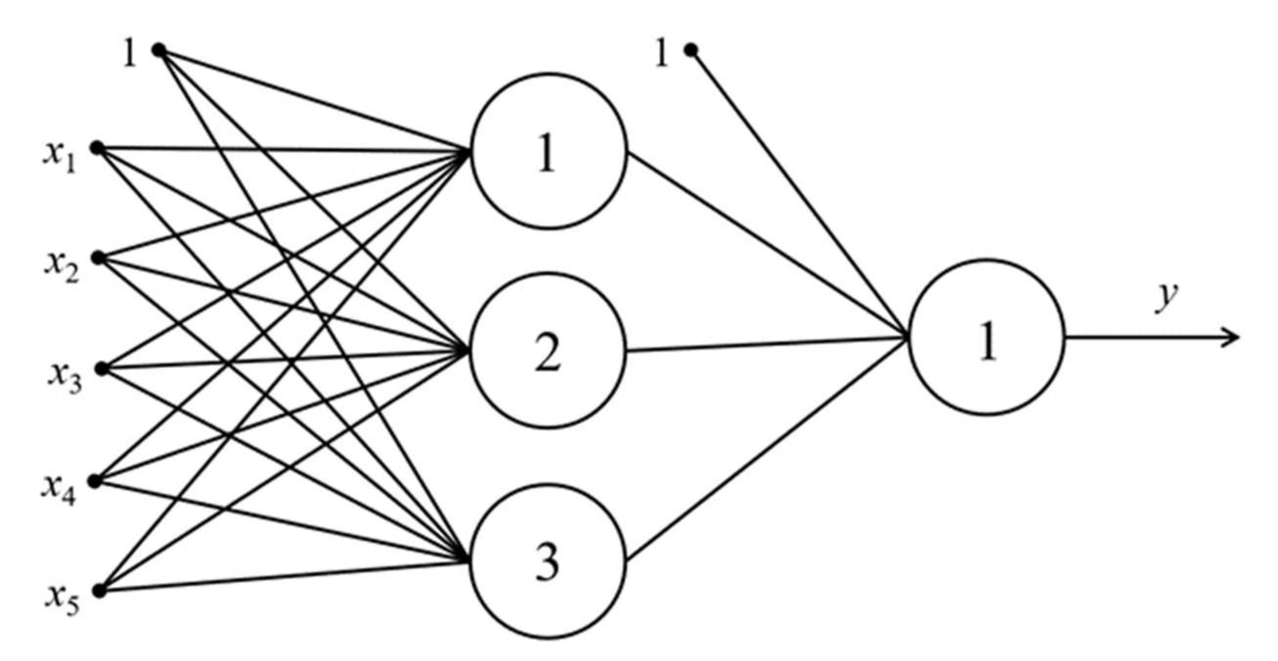
x1, duration of the process, (h);
-
x2, initial concentration of carbohydrate substrate—oligofructose, (g/L);
-
x3, initial concentration of lactic acid, (g/L);
-
x4, initial concentration of acetic acid, (g/L);
-
x5, initial count of bifidobacteria, (logCFU/mL)).
All variables used in the mathematical model were preliminarily converted into a non-dimensional format and normalized within [0; 1] to exclude the influence of scale and measurement units. The count of bifidobacteria was subjected to preliminary logarithmic scaling in order to meet the requirement of data representativeness in all ranges of acceptable values.
One output variable (y) was the dimensionless value of the logarithm of the bifidobacteria count, log CFU/mL), normalized within [0; 1] at the current time corresponding to the duration of the process.
For the ANN mathematical model, data samples taken from the training and testing experiments were relatively small because the described experiment was time-consuming. This led to a number of features related to the mathematical modelling procedure and the interpretation of the obtained results:
-
Limitation on the choice of a number of possible variants for the neural network architecture;
-
Implementation of training and testing algorithms;
-
Various levels of modelling errors for the values of variables from different ranges.

3. Materials and Methods

3.1. The Justification of Choice for ANN Architecture

The limitations discussed above led to the choice of a mathematical modelling tool from two classes of ANN: perceptrons and networks of radial basis functions. At the stage of practical application, both neural networks behave as static networks: the input signal propagates unidirectionally towards the outputs, and they do not have feedback typical for dynamic networks.
Let us take a look at each of these classes in more detail.
Perceptrons are divided into single-layer and multi-layer types. Single-layer perceptrons do not contain hidden layers. Only one neuron layer is the output. They allow the description of simple dependencies. Based on the object specifics we decided not to use single-layer perceptrons because they are not suitable for solving the task.
Multilayer perceptrons make it possible to describe complex and multiple connected dependencies with high accuracy thanks to the presence of one or more hidden layers. However, the complicated network structure leads to a significant increase in the requirements for the size of the training sample, and, as mentioned earlier, this comes into conflict with the capabilities and features of the experiment. Therefore, a two-layer perceptron structure (with one hidden layer) should be considered an optimal solution.
Two-layer perceptrons are an ANN of direct distribution [9]. The number of network inputs corresponds to the number of input variables of the mathematical model and the number of neurons in the output layer; accordingly, the outputs of the neural network corresponding to the number of output variables. The number of hidden neurons may vary depending on the complexity of the connection between inputs and outputs as well as the diversity and quantitative composition of the training sample examples. As a rule, the number of hidden neurons should be greater than the number of output variables. Perceptrons contain neurons of the same type, usually identically tuned, with a sigmoid logistic activation function.
An alternative to perceptrons for solving this task is the use of a neural network of radial basis functions (i.e., a RBF network). A RBF network has a two-layer structure [25] but the neurons in the hidden and output layers differ from each other. The hidden layer is a layer of radial basis functions. A one-dimensional or multidimensional Gaussian function (depending on the dimension of the modelling task) is usually used as an activation function for such neurons. The number of hidden neurons is determined by the number of given interpolation nodes, and the outputs of these neurons represent a measure of the correspondence between the input variables vector to the centres of one of the nodes. The neurons of the second (output) layer make it possible to linearly weigh the outputs of the hidden layer neurons, which in turn makes it possible to calculate the network outputs for the given input combination of variable values.
Both bilayer perceptrons and RBF networks have repeatedly proved their effectiveness in solving various modelling tasks [9,11,25]. In order to finally choose the mathematical approach for modelling, we carried out the preliminary calculations for these two neural network structures, which were equivalent in terms of computing power, using some of the experimental data.
The main criteria for their comparison included: training algorithm, training time, calculation time for the trained neural network, complexity of the structure, volume of calculations, training and testing errors, and principles for choosing network settings. Many of these criteria are interconnected. In the following we provide a comparison of the considered architectures according to the criteria listed above.
Both architectures lean on the principle of supervised training. This principle implies the presence of a training set representing an array of input and output variables matched with each other. In both cases, the goal of training the ANN is to determine values of the weight coefficients at which the calculated output values will be closest to the experimental output values. In the case of two-layer perceptrons, the training algorithm consists of multiple clarifications of weights. The realisation of the algorithm depends on the initial initialization of the weight coefficients and the order in which the training examples are presented. This is greatly manifested in the error backpropagation algorithm [11,26]. In neural networks based on radial basis functions, the weight coefficients of the output layer can definitely be calculated in one calculation cycle using the basic operations of matrix algebra, as the weight coefficients are linearly connected with the output values (and therefore also with the calculation error for each example). These differences in organizing the training algorithm predetermine the possibility of the additional training of two-layer perceptrons when new training vectors appear, and the need for training from the beginning in a similar situation for RBF networks.
Two-layer perceptrons and RBF networks can differ greatly in training time due to the peculiarities of the algorithm organization for choosing weight coefficients. For RBF networks, the training time is very short. In many cases, the training process can be almost instantaneous due to the single calculation cycle. For two-layer perceptrons, the training process can extend for minutes and even hours. In the latter case, the duration of training is very sensitive to the dimension of the task, the network structure, and the size of the training sample. However, the duration of training for two-layer perceptrons does not affect the time of their practical use. Similar to RBF networks, the calculation for a trained perceptron is rapidly performed in a single pass of signals from inputs to outputs.
Practically, these networks do not differ in their structural complexity. Both are two-layer networks with direct signal propagation. In both cases, the nonlinearity of input processing is achieved using an activation function: in RBF networks it is a Gaussian function, while in perceptrons it is a sigmoid logistic function. There is only one significant difference: in two-layer perceptrons, the nonlinear transformation of signals is carried out in both layers, and in RBF networks it is carried out only in the hidden layer. The closeness of the two network structures leads to a minimal, practically insignificant difference in the computation volume.
Both networks are identically sensitive to the volume and representativeness of training data. When the network structure is adequately complex it is better to have more examples of training samples to diminish fewer training and testing errors. It is practically impossible to take into account the representativeness of data in the training sample when setting up two-layer perceptrons, but it can be done by adjusting the density of interpolation nodes in the hidden layer for RBF networks. Nevertheless, this will not affect the low level of data accuracy in ranges where the density of the original data is quite low.
A coefficient with an argument in the exponent (a saturation parameter of the activation function) is used as one of the main settings for both ANN architectures. A larger absolute value of the coefficient increases the rate of change of the activation function for certain values of the argument and thus allows you to more clearly, selectively respond to its change. Conversely, if the saturation parameter is closer to zero, the influence of the activation function argument is less. When choosing the saturation parameter, it is important to correctly find its level. A value that is too large will lead to the minimization of the range of argument values, which affect the calculation result. A value that is too small will lead to blur and uncertainty in this range.
The generalized results of the comparison of two architectures are shown in Table 1.
The results of the comparison of modelling ability for two-layer perceptrons and RBF networks are shown in Figure 1. The comparison procedure was conducted for one bifidobacteria metabolite, lactic acid, with an OF concentration of 5 g/L. A sample of 88 training examples was considered which describes the change in the lactic acid concentration during the fermentation process. A two-layer perceptron with five neurons in the hidden layer and a neural network of radial basis functions with five hidden radial elements were considered and compared. In both cases, the activation function saturation parameter had a value of 2.0. The testing was carried out on 10 examples. As a result, the root-mean-square errors (RMSE) (Equation (1)) were calculated to compare experimental and modelling results for test samples: for the RBF network the RMSE was 10.7%, and for the perceptron it was 5.97%.
E ˜ = 1 N K k = 1 N j = 1 K y ˜ j k Π y ˜ j k p 2 100 % ,
where K is the number of neural network output variables and N is the number of sample examples.
Considering the complexity of the task being solved and the traditionally high level of errors of mathematical models, the two-layer perceptron was chosen as the mathematical modelling tool, as on average it gave half the error for structures equivalent in ANN complexity.

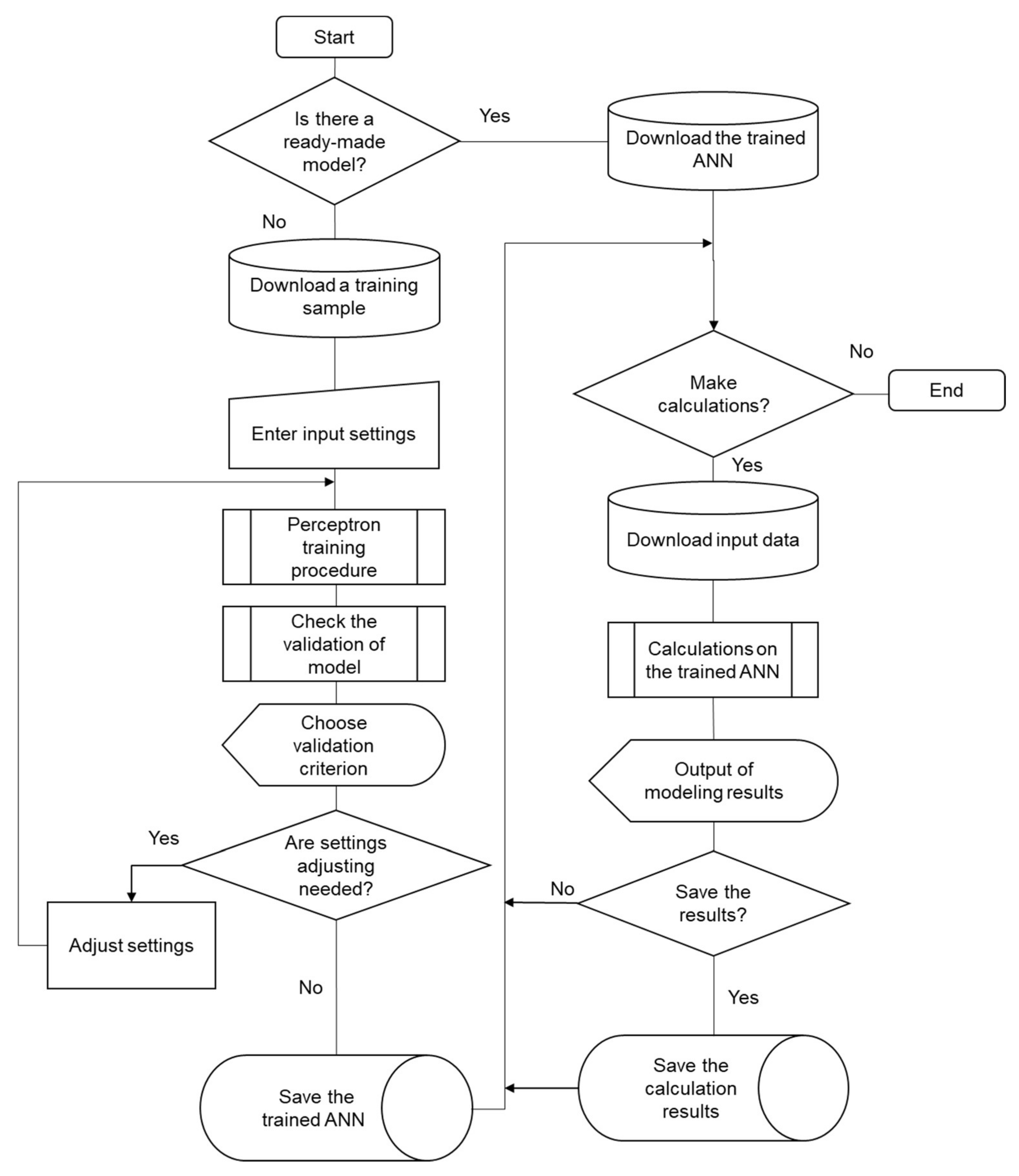
3.2. The Procedure of Settings and Structure Choice for Two-Layer Perceptron. Description of the Algorithm

To obtain a mathematical model in the form of a two-layer perceptron, it is necessary to optimize its structure, neuron settings, and training algorithm. The number of input and output variables and one hidden layer were already determined, and must remain unchanged. Only the number of hidden neurons can change in the network structure. It is required to select the saturation parameter (the coefficient under the exponent) for the sigmoid logistic activation function of neurons, which was previously chosen. The adjusted parameter of the training algorithm was the coefficient of the correction rate of synaptic coefficients.
Figure 2 illustrates the operation algorithm in two cases. The first case is the use of the previously developed and tuned mathematical model (right side of the figure). The second case considers the variant when the user has no such model and has to develop a new one using the corresponding algorithm for choosing the optimal settings and structure of the perceptron (left side).
  • If there is no ready, previously configured and trained neural network for calculations, a training sample is formed from the experimental data.
  • The initial value of the saturation parameter, the number of hidden neurons and the training rate coefficient are entered.
  • The perceptron is trained according to the backpropagation algorithm.
  • For the trained perceptron, the validity of the model is estimated for training and testing samples by the calculation of the root-mean-square errors. The share of correctly recognized examples is also defined.
  • If the error values exceeded the maximum allowable value of the training algorithm settings, the activation function and/or structure of the perceptron is corrected, and the algorithm continues from step 3.
  • If suitable network settings are found, they are stored together with the obtained synaptic coefficient values as a mathematical model for further use.
  • If it is necessary to use this model for input data, the signal propagates in the forward direction from the inputs to the outputs of the perceptron. The output values are used for their intended purpose.

4. Results and Discussion

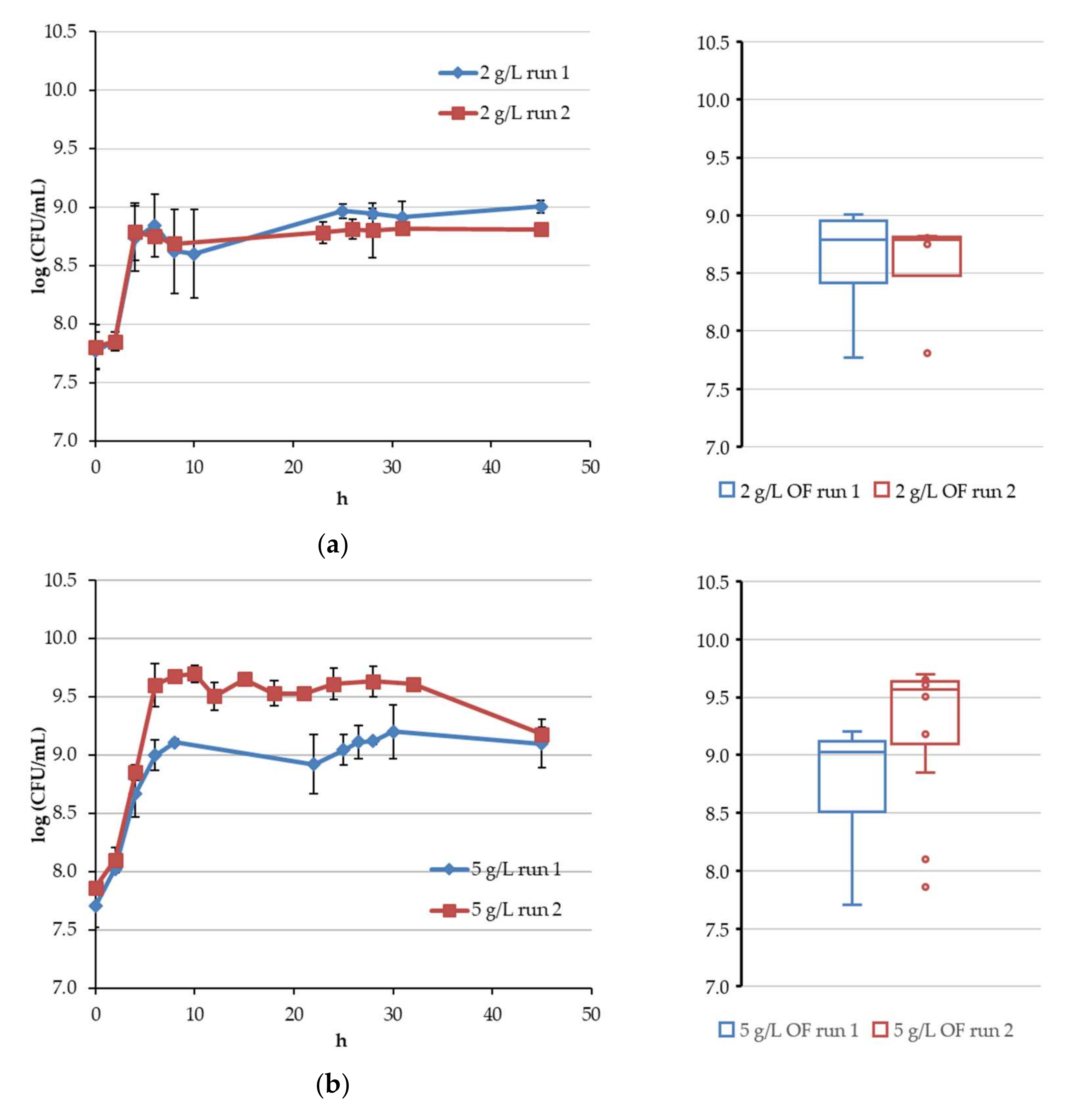
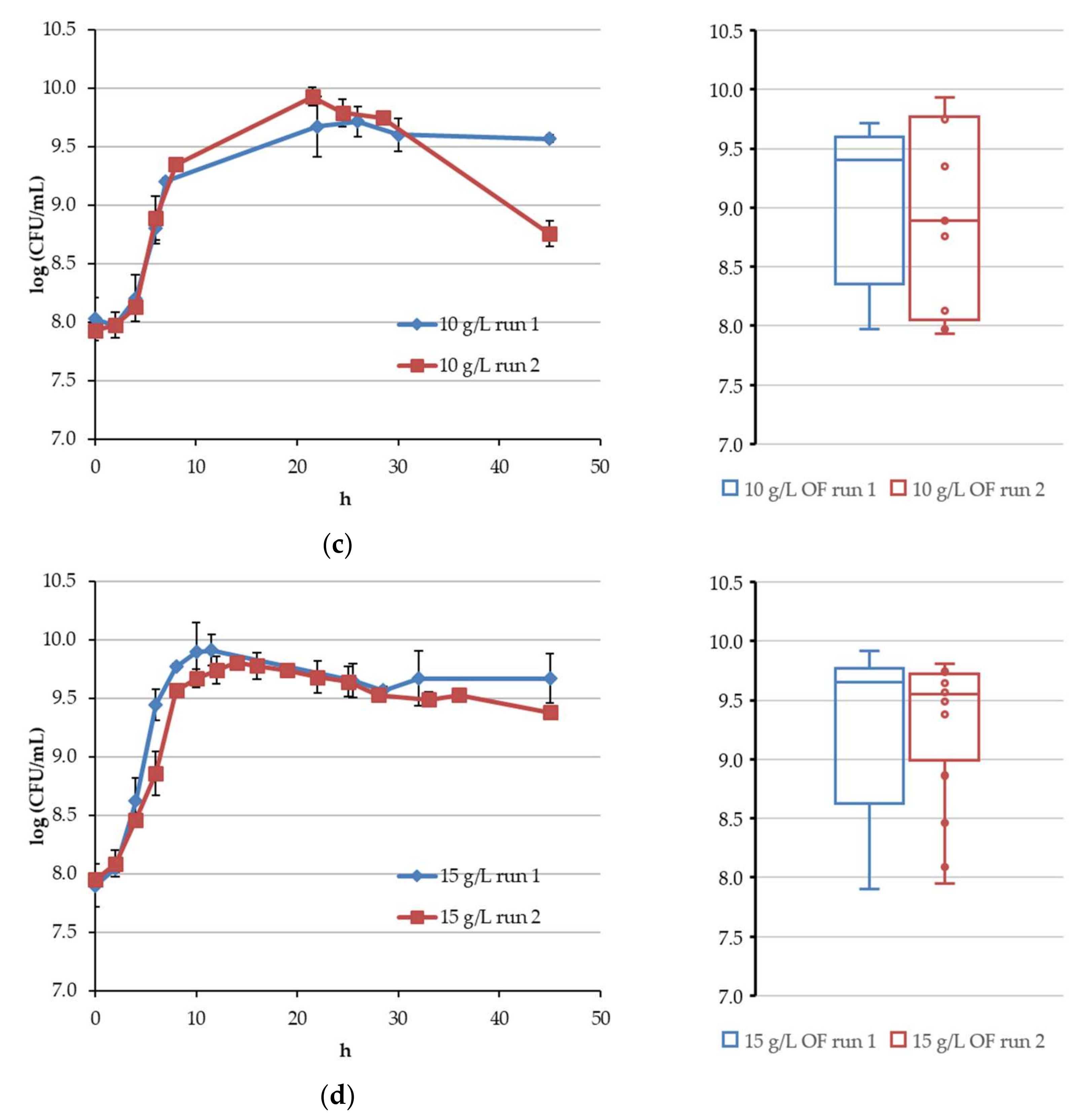
4.1. Continuous Fermentation of Bifidobacteria in Simulated Descending Colon Conditions

The results of the experiments made it possible to obtain preliminary information about the development of the microbial population of bifidobacteria during colonization of the intestinal biotope, and to calculate the necessary constants of the kinetic model [24]. In this study, the obtained experimental data were also used to create and train the ANN. First, we will discuss the main biological results. The study was carried out in two runs for each considered concentration of oligofructose (Figure 3), and the measurements of the bifidobacteria count, acid concentration and substrate consumption were taken in three repetitions (Figure 3). At all concentrations, two stages were observed. At the first stage (from 5 to 10 h) there was an increase in the bifidobacteria count with an excess of substrate input, in comparison with its consumption and the removal of inhibitors at a rate exceeding their formation. At the next stage of dynamic equilibrium, the rates of substrate input and consumption, as well as the rates of product formation and removal, became equal. As a result, the bifidobacteria count remained practically constant. At the same time, the stationary values for the minimum OF concentration were noticeably lower than at high values. The resulting data appeared to be robust for ANN training.
The specific growth rate naturally had values close to zero in the stationary phase for continuous fermentation (Supplementary Figure S1). It should be noted that the values of the average specific growth rates obtained by calculations between two points are approximate, and only conditionally reflect the real influence of the parameters on the system, which must be taken into account. In fact, according to the obtained kinetic model [24], there is an equilibrium between the real growth rate, the rate of death, and the rate of dilution during continuous fermentation in a stationary state for bifidobacteria.

4.2. Results of Algorithm Investigation

Let us illustrate the results obtained using the considered algorithm. Figure 4 shows the change in the perceptron training error, depending on the number of hidden neurons with the other fixed network and training algorithm settings. The training sample comprised 123 examples.
It can be seen from the figure that when the number of hidden neurons changed from 3 to 5, the error decreased slightly (by less than 1%). At the same time, the number of connections (synapses) and hence the weight coefficients optimized in the training process, was 22 in the case of 3 neurons and 36 for 5 neurons in the hidden layer. The use of a smaller number of hidden neurons is preferable, as this simplifies the model, reduces the calculations and allows the perceptron to more easily generalize the initial data.
The structure of the chosen perceptron with three hidden neurons is shown in Figure 5.
During the optimization of the saturation parameter, its various values were considered in the range from 0.5 to 3.0 with a step of 0.5. The value of 2.0 was chosen for further use based on the results of comparing training and testing errors.
We studied the influence of the training rate coefficient on the quality of the resulting neural network model, and found that the use of any constant rate coefficient was not effective. At high values of the training rate coefficient (0.25 and greater), the localization area of a good solution was identified quite quickly, but the solution could not be stabilized near the minimum error due to the high values of the coefficient, and hence due to the strong correction of the weights in the later training epochs. At low values of the training rate coefficient (0.1 or less), the training process could continue for an unacceptably long period. In addition, the probability of the solution stabilization near the error local minimum was greatly increased and the neural network model could be of poor quality.
Given the above, the optimal training strategy was to use a decreasing rate from 0.50 to 0.03. Figure 6 shows the change in the training error from the ordinal number of the epoch with the decreasing weight correction rate coefficient.

4.3. Features and Algorithm for Testing a Two-Layer Perceptron with a Small Sample Size

Traditionally, in neural network modelling, the initial data sample is divided into training and testing parts. At the end of the training process, the network error is calculated only from the test cases. Thus, it becomes possible to compare training and testing errors and make an assumption about how the model will behave in new, previously unseen input variable combinations. With minimum error discrepancy, it is concluded that the trained network will behave in a similar way at the stage of its practical operation.
As mentioned above regarding long and expensive experiments, the size of the initial sample is often not very large, and the ANN model should consider all data during training in order to avoid decreasing the quality of the resulting model. In order to obtain a model of the required quality, and to be able to adequately test it, we proposed a special algorithm that makes it possible to use all available examples for independent testing. The block diagram of this algorithm is shown in Figure 7.
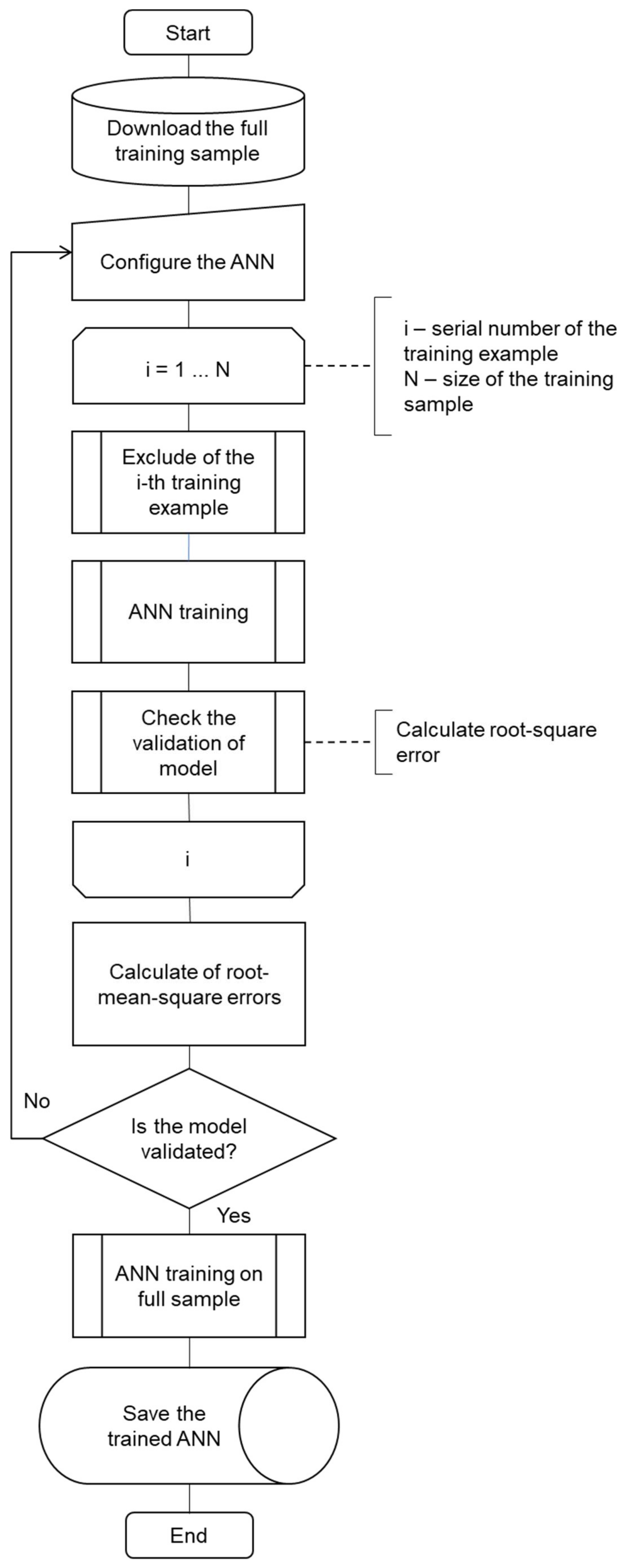
  • All examples needed to obtain a neural network model are loaded from the experimental results.
  • The model settings are selected based on the researcher’s experience.
  • The cycle using all examples of the sample is organized. During the cycle:
    -
    One of the examples is excluded from the sample in a definite order;
    -
    The neural network is trained on the basis of the error backpropagation algorithm;
    -
    The correspondence errors between experimental and modelling results of the model are evaluated.
When moving to the next cycle step, the previously excluded example is returned to the sample, and the next one based on its serial number is excluded.
4.
At the end of the cycle, the root-mean-square errors are calculated using experimental and modelling results of the trained networks.
5.
If the root-mean-square errors are satisfactory, a neural network with the same structure and settings is already trained on the full sample (without excluding examples from it), and the resulting model is saved for further use.
6.
If the errors obtained in step 4 were unsatisfactory, the procedure is repeated from step 2 with new settings.
The described procedure can be successfully integrated into the structure of the algorithm shown in Figure 2, making it possible to choose the optimal structure and settings of neurons for the ANN model.

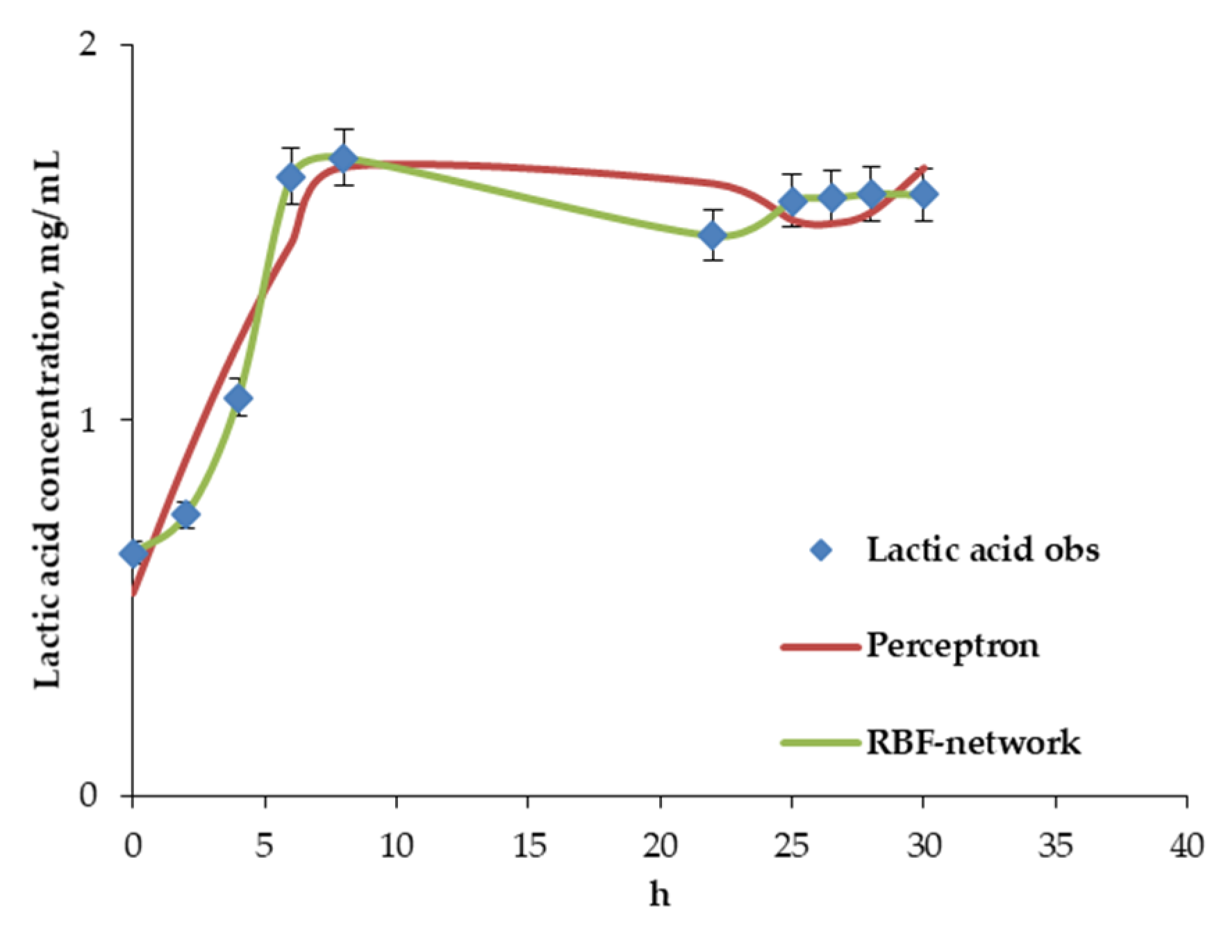
4.4. Artificial Neural Network Model of Continuous Bifidobacteria Monoculture at Low Flow Rate

As a result of applying the described principles of neural network modelling and the algorithms presented in Figure 2 and Figure 7, a mathematical model was obtained that describes the metabolism of bifidobacteria in monoculture at a low flow rate. The training sample of 123 examples included five of the previously listed input variables and one output variable.
The neural network corresponding to Figure 5 contained three hidden neurons. The saturation parameter was 2.0. The training strategy with the decreasing rate coefficient was used. As a result, the synaptic coefficient values given in Table 2 were obtained.
Index 0 corresponds to the bias coefficient characterizing the connection weight for a fictitious single input to a neuron.
The states of neurons in the hidden layer are determined by the relation:
S j = i = 0 5 w i j x i .
The outputs of neurons in the hidden layer are calculated as follows:
y j = 1 1 + e 2 S j .
Based on the values of the hidden layer outputs, the state of a single neuron in the output layer can be calculated:
S = j = 0 3 w j 1 y j .
The output of the neural network (and, accordingly, the model) is defined as:
y = 1 1 + e 2 S .
Since the neural network works with normalized values, in order to interpret the simulation results and make decisions based on them, denormalization should be performed, which means bringing the data to the original scale and measurement units.
Example modelling results for the bifidobacteria growth in OF concentrations of 2, 5, 10 and 15 g/L are presented in Figure 8. The root-mean-square errors for the correspondence between experimental and modelling results ranged from 4.71 to 7.89% for the ANN with three neurons, and from 4.24 to 9.80% for the model with two neurons, as the former is simpler. The difference of approximately half a percent in favour of the two-neuron structure is explained not so much by the difference in the model structure, but by the different values of the weight coefficients during the initialization of the network and, accordingly, by the different localization of the optimum. In each case, the minimal value of RMSE was obtained for the experiments in 5 g/L of OF.
Analysis of the calculation results indicated that the application of ANN models based on two-layer perceptrons made it possible to obtain good correspondence between experimental and predicted data for models with both two and three neurons. The calculations in this study were made only for bifidobacteria monoculture.
Similar investigations were considered in related studies [27,28,29]. Thus, it is possible to conclude that the presence of one hidden layer in the perceptron structure was the optimal solution, since an increase in the number of hidden layers is unjustified, primarily due to the small volume of experimental data (training sample). Additionally, the absence of a hidden layer led to higher errors and, consequently, poor modelling ability for single-layer networks.
Complicating the structure of the ANN by adding hidden neurons (as shown in [27]) is possible only with a larger training set. While maintaining the sample volume and a larger number of hidden neurons, the question of the generalization capabilities of the network and the correctness of its operation for combinations of variables on which the neural network was not actually trained (as in [28]) remains open. Besides, it was confirmed that the use of an ANN as a mathematical model for microbiological and biotechnological processes can reduce the modelling error in comparison with other methods for solving similar problems [30].
On the other hand, the results can be accepted as a preliminary step for gut microbial community behaviour and dynamic models for their prediction. Although ANNs and machine learning are commonly used in biomedical tasks for big data processing and evaluating the impact of microbiota on human health and disease [31,32], few studies are dedicated to intra-community interaction. Synthetic communities can be applied for data collection. It was previously demonstrated that the long short-term memory framework (as a type of ANN) could outperform a kinetic model (Lotka–Volterra) in the investigation and prediction of the stability and dynamics of a synthetic gut microbial community [33]. In [34] a generalized Lotka–Volterra model joining a differential neural network (DNN) was used in order to estimate the interaction between representatives of gut microbiota. The promised approach was proposed and made it possible to define the bidirectional interactions in the mixed microbial culture. The prospects of our approach in the future involve the study and modelling of co-culture and faecal in vitro culture (e.g., a three-stage continuous model). It is clear that these objects maintain a huge number of relations (many of which cannot be measured instrumentally) and will be a promising object for neural network modelling.

5. Conclusions

Given the modelling interactions between both the microbial community members and the host, modern approaches should consider a large number of factors and interactions. Artificial neural networks are an alternative tool for kinetic modelling that have already been widely used in biology. Thus, the results obtained for continuous bifidobacteria monoculture in simulated colon conditions indicate a good level of model validation that describes microbial metabolism. Taking into account these results, as well as those of other studies, it can be concluded that the use of two-layer perceptron artificial neural networks makes it possible to efficiently solve mathematical modelling problems for similar systems. The modelling of the metabolism of bifidobacteria in the intestine in the presence of other members of the microbial gut community is a promising area of research. For synthetic or faecal microbial communities, both neural network and classical models (e.g., kinetics or Lotka–Volterra) can be useful. In the latter case, however, the determination of the constants of the kinetic equations or bidirectional interactions is required. This is beyond the scope of the present study, but could be carried out in the future. A system of neural network models describing various sections of the gastrointestinal tract could be useful for the comprehensive description of the functioning of the human digestive system.

Supplementary Materials

The following supporting information can be downloaded at: https://0-www-mdpi-com.brum.beds.ac.uk/article/10.3390/data7050058/s1, Figure S1: The flow diagram of the descending colon in vitro simulation unit; Figure S2: The observed (apparent) specific growth rates calculated by the equation below for bifidobacteria monoculture at OF concentrations.

Author Contributions

Conceptualization, S.D., B.K. and E.G.; methodology, S.D.; software, S.D., I.M. and P.P.; validation, I.M. and Y.L.; formal analysis, P.P.; investigation, B.K. and S.E.; resources, B.K. and S.E.; data curation, E.G.; writing—original draft preparation, S.D. and E.G.; writing—review and editing, S.D., B.K. and E.G.; visualization, Y.L. and P.P.; supervision, N.M. and V.P.; project administration, B.K.; funding acquisition, B.K. All authors have read and agreed to the published version of the manuscript.

Funding

The present study was sponsored by Russian Science Foundation (Project № 17-79-20365).

Institutional Review Board Statement

Not applicable.

Informed Consent Statement

Not applicable.

Data Availability Statement

Data are contained within the article and Supplementary Materials.

Conflicts of Interest

The authors declare no conflict of interest.

References

  1. Bridgman, S.L.; Kozyrskyj, A.L.; Scott, J.A.; Becker, A.B.; Azad, M.B. Gut microbiota and allergic disease in children. Ann. Allergy Asthma Immunol. 2016, 116, 99–105. [Google Scholar] [CrossRef] [PubMed] [Green Version]
  2. Gilbert, J.A.; Blaser, M.J.; Caporaso, J.G.; Jansson, J.K.; Lynch, S.V.; Knight, R. Current understanding of the human microbiome. Nat. Med. 2018, 24, 392–400. [Google Scholar] [CrossRef] [PubMed]
  3. Oh, B.; Boyle, F.; Pavlakis, N.; Clarke, S.; Guminski, A.; Eade, T.; Lamoury, G.; Carroll, S.; Morgia, M.; Kneebone, A.; et al. Emerging Evidence of the Gut Microbiome in Chemotherapy: A Clinical Review. Front. Oncol. 2021, 11, 706331. [Google Scholar] [CrossRef]
  4. Hill, C.; Guarner, F.; Reid, G.; Gibson, G.R.; Merenstein, D.J.; Pot, B.; Morelli, L.; Canani, R.B.; Flint, H.J.; Salminen, S.; et al. Expert consensus document. The International Scientific Association for Probiotics and Prebiotics consensus statement on the scope and appropriate use of the term probiotic. Nat. Rev. Gastroenterol. Hepatol. 2014, 11, 506–514. [Google Scholar] [CrossRef] [PubMed] [Green Version]
  5. Swanson, K.S.; Gibson, G.R.; Hutkins, R.; Reimer, R.A.; Reid, G.; Verbeke, K.; Scott, K.P.; Holscher, H.D.; Azad, M.B.; Delzenne, N.M.; et al. The International Scientific Association for Probiotics and Prebiotics (ISAPP) consensus statement on the definition and scope of synbiotics. Nat. Rev. Gastroenterol. Hepatol. 2020, 17, 687–701. [Google Scholar] [CrossRef] [PubMed]
  6. Danne, C.; Rolhion, N.; Sokol, H. Recipient factors in faecal microbiota transplantation: One stool does not fit all. Nat. Rev. Gastroenterol. Hepatol. 2021, 18, 503–513. [Google Scholar] [CrossRef] [PubMed]
  7. Gibson, G.R.; Cummings, J.H.; Macfarlane, G.T. Use of a three-stage continuous culture system to study the effect of mucin on dissimilatory sulfate reduction and methanogenesis by mixed populations of human gut bacteria. Appl. Environ. Microbiol. 1988, 54, 2750–2755. [Google Scholar] [CrossRef] [Green Version]
  8. Macfarlane, G.T.; Macfarlane, S.; Gibson, G.R. Validation of a Three-Stage Compound Continuous Culture System for Investigating the Effect of Retention Time on the Ecology and Metabolism of Bacteria in the Human Colon. Microb. Ecol. 1998, 35, 180–187. [Google Scholar] [CrossRef]
  9. Rosenblatt, F. The Perceptron: A Probabilistic Model For Information Storage and Organization in the Brain. Psychol. Rev. 1958, 65, 386–408. [Google Scholar] [CrossRef] [Green Version]
  10. Wasserman, P.D.; Schwartz, T. Neural networks. II. What are they and why is everybody so interested in them now? IEEE Expert 1988, 3, 10–15. [Google Scholar] [CrossRef]
  11. Schmidhuber, J. Deep Learning in Neural Networks: An Overview. Neural Netw. 2015, 61, 85–117. [Google Scholar] [CrossRef] [PubMed] [Green Version]
  12. Açıcı, K.; Asuroglu, T.; Erdas, C.B.; Ogul, H. T4SS Effector Protein Prediction with Deep Learning. Data 2019, 4, 45. [Google Scholar] [CrossRef] [Green Version]
  13. Zhu, N.; Wang, K.; Zhang, S.; Zhao, B.; Yang, J.; Wang, S. Application of artificial neural networks to predict multiple quality of dry-cured ham based on protein degradation. Food Chem. 2021, 344, 128586. [Google Scholar] [CrossRef] [PubMed]
  14. Kovarova-Kovar, K.; Gehlen, K.; Kunze, A.; Keller, T.; von Daniken, R.; Kolb, M.; van Loon, A.P.G.M. Application of model-predictive control based on artificial neural networks to optimize the fed-batch process for riboflavin production. J. Biotechnol. 2000, 79, 39–52. [Google Scholar] [CrossRef]
  15. Oliveira, R.; Peres, J.; de Azevedo, S.F. Hybrid modelling of fermentation processes using artificial neural networks: A study of identification and stability. IFAC Proc. Vol. 2004, 37, 195–200. [Google Scholar] [CrossRef]
  16. Setoodeh, P.; Jahanmiri, A.; Eslamloueyan, R. Hybrid neural modeling framework for simulation and optimization of diauxie-involved fed-batch fermentative succinate production. Chem. Eng. Sci. 2012, 81, 57–76. [Google Scholar] [CrossRef]
  17. Ignova, M.; Montague, G.A.; Ward, A.C.; Glassey, J.; Kornfeld, G.; Thomas, C.R. Hybrid modeling and optimisation of industrial fed batch fermentation process. IFAC Proc. Vol. 1998, 31, 271–276. [Google Scholar] [CrossRef]
  18. Pendashteh, A.R.; Fakhru’l-Razi, A.; Chaibakhsh, N.; Abdullah, L.C.; Madaeni, S.S.; Abidin, Z.Z. Modeling of membrane bioreactor treating hypersaline oily wastewater by artificial neural network. J. Hazard. Mater. 2011, 192, 568–575. [Google Scholar] [CrossRef]
  19. Antwi, P.; Lic, J.; Meng, J.; Deng, K.; Quashie, F.K.; Li, J.; Boadi, P.O. Feedforward neural network model estimating pollutant removal process within mesophilic upflow anaerobic sludge blanket bioreactor treating industrial starch processing wastewater. Bioresour. Technol. 2018, 257, 102–112. [Google Scholar] [CrossRef] [Green Version]
  20. Jianfei, L.; Weitie, L.; Xiaolong, C.; Jingyuan, L. Optimization of Fermentation Media for Enhancing Nitrite-oxidizing Activity by Artificial Neural Network Coupling Genetic Algorithm. Chin. J. Chem. Eng. 2012, 20, 950–957. [Google Scholar]
  21. Williams, C.F.; Walton, G.E.; Jiang, L.; Plummer, S.; Garaiova, I.; Gibson, G.R. Comparative analysis of intestinal tract models. Annu. Rev. Food Sci. Technol. 2015, 6, 329–350. [Google Scholar] [CrossRef] [PubMed]
  22. Tojo, R.; Suárez, A.; Clemente, M.G.; de los Reyes-Gavilán, C.G.; Margolles, A.; Gueimonde, M.; Ruas-Madiedo, P. Intestinal microbiota in health and disease: Role of bifidobacteria in gut homeostasis. World J. Gastroenterol. 2014, 7, 15163–15176. [Google Scholar] [CrossRef] [PubMed]
  23. Organji, S.; Abulreesh, H.; Elbanna, K.; Osman, G.; Khider, M. Occurrence and characterization of toxigenic Bacillus cereus in food and infant feces. Asian Pac. J. Trop. Biomed. 2015, 5, 510–514. [Google Scholar] [CrossRef] [Green Version]
  24. Evdokimova, S.A.; Karetkin, B.A.; Guseva, E.V.; Gordienko, M.G.; Khabibulina, N.V.; Panfilov, V.I.; Menshutina, N.V.; Gradova, N.B. A study and modelling of Bifidobacteria and Bacilli Co-culture Continuous Fermentation under distal intestine simulated conditions. Microorganisms 2022, 10, 929. [Google Scholar] [CrossRef]
  25. Moody, J.; Darken, C.J. Fast learning in networks of locally tuned processing units. Neural Comput. 1989, 1, 281–294. [Google Scholar] [CrossRef]
  26. Dreyfus, S.E. Artificial neural networks, back propagation, and the Kelley-Bryson gradient procedure. J. Guid. Control Dyn. 1990, 13, 926–928. [Google Scholar] [CrossRef]
  27. Meena, G.S.; Gupta, S.; Majumdar, G.C.; Banerjee, R. Growth Characteristics Modeling of Bifidobacterium bifidum Using RSM and ANN. Braz. Arch. Biol. Technol. Int. J. 2011, 54, 1357–1366. [Google Scholar] [CrossRef] [Green Version]
  28. Meena, G.S.; Majumdar, G.C.; Banerjee, R.; Kumar, N.; Meena, P.K. Growth Characteristics Modeling of Mixed Culture of Bifidobacterium bifidum and Lactobacillus acidophilus using Response Surface Methodology and Artificial Neural Network. Braz. Arch. Biol. Technol. 2014, 57, 962–970. [Google Scholar] [CrossRef] [Green Version]
  29. Amiri, Z.R.; Khandelwal, P.; Aruna, B.R. Development of acidophilus milk via selected probiotics & prebiotics using artificial neural network. Adv. Biosci. Biotechnol. 2010, 1, 224–231. [Google Scholar] [CrossRef] [Green Version]
  30. García-Gimeno, R.M.; Hervás-Martínez, C.; Barco-Alcalá, E.; Zurera-Cosano, G.; Sanz-Tapia, E. An Artificial Neural Network Approach to Escherichia coli O157:H7 Growth Estimation. J. Food Sci. 2003, 68, 639–645. [Google Scholar] [CrossRef]
  31. Ghannam, R.B.; Techtmann, S.M. Machine learning applications in microbial ecology, human microbiome studies, and environmental monitoring. Comput. Struct. Biotechnol. J. 2021, 19, 1092–1107. [Google Scholar] [CrossRef] [PubMed]
  32. Marcos-Zambrano, L.J.; Karaduzovic-Hadziabdic, K.; Loncar Turukalo, T.; Przymus, P.; Trajkovik, V.; Aasmets, O.; Berland, M.; Gruca, A.; Hasic, J.; Hron, K.; et al. Applications of Machine Learning in Human Microbiome Studies: A Review on Feature Selection, Biomarker Identification, Disease Prediction and Treatment. Front. Microbiol. 2021, 12, 634511. [Google Scholar] [CrossRef] [PubMed]
  33. Baranwal, M.; Clark, R.L.; Thompson, J.; Sun, Z.; Hero, A.O.; Venturelli, O. Deep Learning Enables Design of Multifunctional Synthetic Human Gut Microbiome Dynamics. bioRxiv 2021. submitted. [Google Scholar] [CrossRef]
  34. Gradilla-Hernández, M.S.; García-González, A.; Gschaedler, A.; Herrera-López, E.J.; González-Avila, M.; García-Gamboa, R.; Montes, C.Y.; Fuentes-Aguilar, R.Q. Applying Differential Neural Networks to Characterize Microbial Interactions in an Ex Vivo Gastrointestinal Gut Simulator. Processes 2020, 8, 593. [Google Scholar] [CrossRef]
Figure 1. The comparison of modelling ability for two-layer perceptrons and RBF networks based on the modelling results for the change of the lactic acid concentration.
Data 07 00058 g001
Figure 2. Block diagram of the algorithm for choosing the optimal settings, the structure of the perceptron (left side) and using a previously developed and tuned mathematical model (right side).
Data 07 00058 g002
Figure 3. Within-run reproducibility and between-run repeatability of bifidobacteria count in simulated descending colon fermentation conditions. Growth curves (left) and box plots (right) for continuous fermentation with 2 g/L (a), 5 g/L (b), 10 g/L (c) and 15 g/L (d) of oligofructose in feed.
Data 07 00058 g003aData 07 00058 g003b
Figure 4. The correspondence of training error with the number of neurons in the hidden layer.
Data 07 00058 g004
Figure 5. The structure of a two-layer perceptron with 3 neurons in the hidden layer.
Data 07 00058 g005
Figure 6. Error change during the perceptron training process.
Data 07 00058 g006
Figure 7. Block diagram of the algorithm for testing a neural network with a small initial sample.
Data 07 00058 g007
Figure 8. Count of bifidobacteria monoculture experimentally observed (Xobs) and predicted by the two-layer perceptron model (Xpred) under OF concentrations of 2 g/L (a), 5 g/L (b), 10 g/L (c) and 15 g/L (d) calculated for 2 and 3 neurons.
Data 07 00058 g008aData 07 00058 g008b
Table 1. Comparison of the influence of two-layer perceptrons and RBF networks on modelling results.
Comparison CriterionTwo-Layer PerceptronsRBF Networks
Organization of the training algorithmMultiple repetitions of the training cycleSingle calculation of weight coefficients
Possibility of additional trainingYesNo
Unambiguity of training results NoYes
Time of ANN training processShortLong
Application time of trained ANNQuicklyQuickly
Number of layers with non-linear signal conversionTwoOne
Possibility to take training data density into accountNoYes
Table 2. Values of synaptic coefficients for the hidden layer neurons (wij) and single output layer neuron (wj1).
Input Number (i)Number of Hidden Neurons (j)
123
00.1342.9364.432
117.3119.4870.449
2−1.473−3.458−2.244
3−0.0653.448−1.796
40.3145.705−0.867
50.395−8.5590.626
Number of Output Neurons (j)
0123
1.8022.226−0.660−3.191
Publisher’s Note: MDPI stays neutral with regard to jurisdictional claims in published maps and institutional affiliations.

