4.1. Multimodal Visualisation
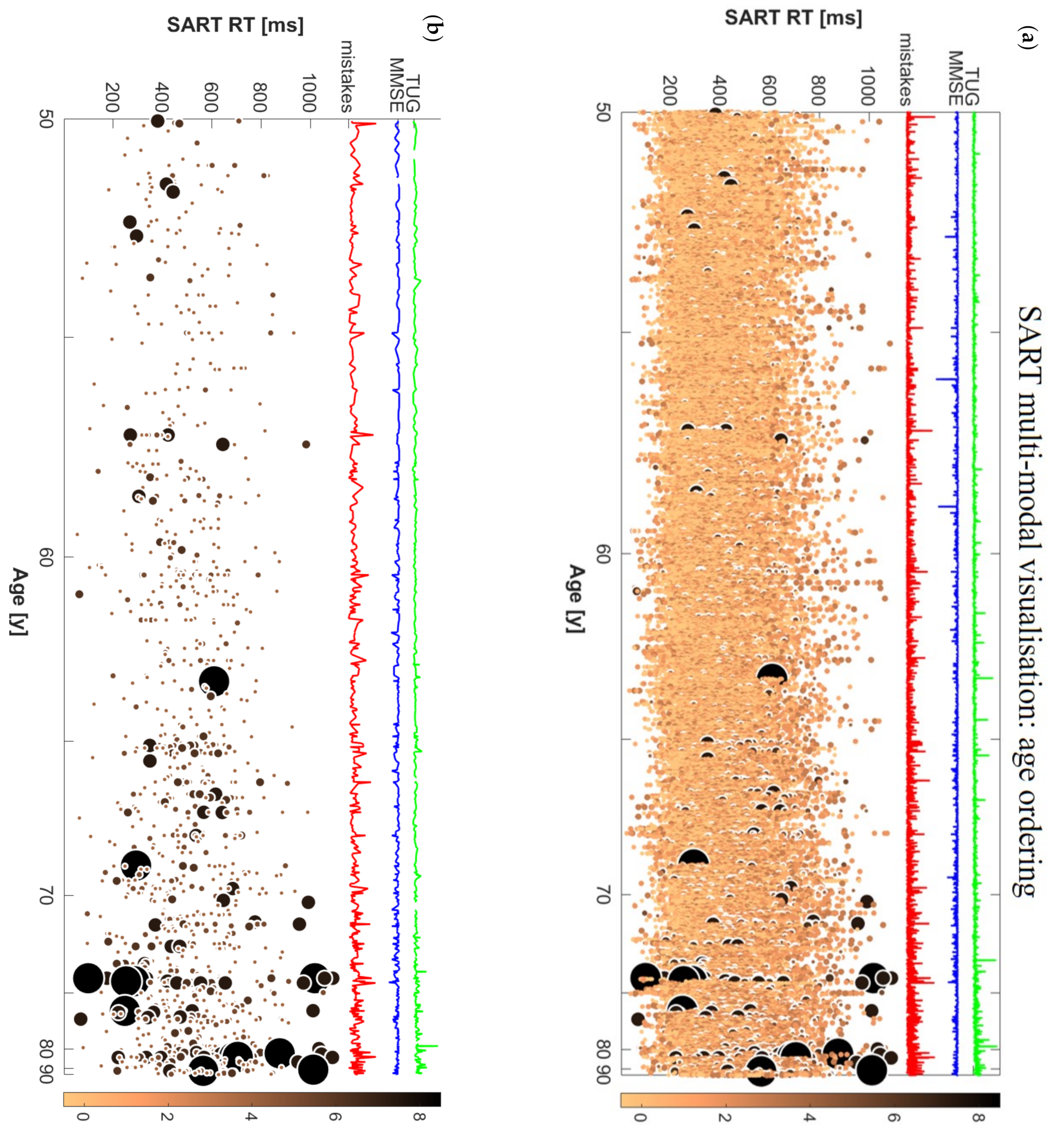
In the present study, we devised a new methodology for the multimodal visualisation of big repeated-measures data with continuous variable ordering and categorical stratification, and we exemplified this with the case of raw SART performance data, accompanied by MMSE and TUG values, sorted by age, and stratified by baseline TUG performance.
By using this novel type of visualisation, clinicians could gain a deeper understanding as to how a complex repeated-measures dataset is articulated across different subjects and across repeated measures (SART trials in this case). Moreover, using the ordering of a continuous variable (age in this case) in the whole dataset (
Figure 1) and within each category (
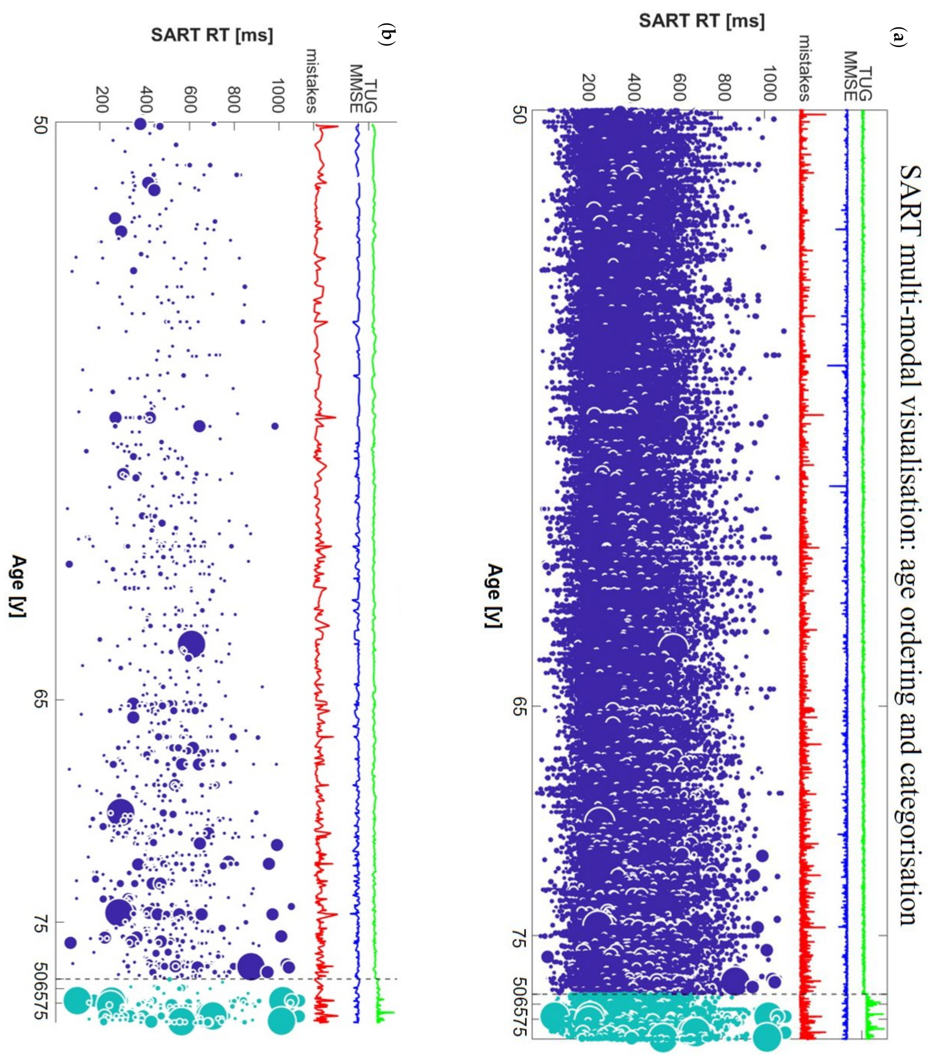
Figure 2) allows one to compare the performance of different subjects by age and to formulate hypotheses that can then be tested with formal statistical analyses. Furthermore, by using the threshold for bad performance (
Figure 1b and
Figure 2b) one can more clearly visualise their distribution across subjects and RTs. This could be the first step in the formulation of a new model to assign cognitive scores to different individuals based on the co-existence of a wide range of different types of parameters.
The visualisations helped us quickly appreciate that bad performances were rare in younger participants (i.e., in their 50s) and concentrated around lower RTs, while in older subjects (i.e., in their 70s and 80s), a wider distribution of bad performances was suggested across a wider range of RTs. By using the thresholding visualisation method, we were able to gain a more focused insight into the participants who had bad SART performances and cross-inspect them with corresponding global parameters of clinical interest such as the total number of SART mistakes, MMSE, and TUG values.
Indeed, the most important characteristic of our visualisation method is the possibility to rapidly visualise raw data and gain immediate insights as to the possible correlations with different kinds of parameters. This multimodal raw data inspection can help visually identify anomalies and outliers in the data, in a way that is diluted and often undetected in traditional designs based on average measures. For example, a high peak in the total mistakes line can be due to one bad performance or multiple performances with just 1 or 2 mistakes, which, in our case would not be labelled as “bad performance” since our threshold required 4 mistakes for the definition of a “bad performance”. The superimposed MMSE and TUG curves further underscore multi-modality by providing a global cognitive and mobility score for each participant. The possibility to look at them together with the whole distribution of SART RT values (not just derivative global variables for SART) can provide a more nuanced understanding of the combined cognitive and mobility status of an individual.
Raw data visualisation can therefore support the generation of multiple novel hypotheses involving the relationship between test performance features and other modalities of clinical interest. For example, in our visualisations it was clear that longer TUG times corresponded to higher concentrations of bad performances, and even to the biggest spots among bad performances, i.e., those with very high number of mistakes (biggest light blue spots in
Figure 2b). Moreover, we could notice that ‘dips’ in MMSE seemed to have a very modest association with SART RT performance [
51]. Not only were the lowest MMSE scores generally not in correspondence with the high number of total SART mistakes, they were not even present among participants with bad performances, as can be seen comparing panels (a) and (b) in
Figure 2. Therefore, we directed our interest towards investigating possible associations between SART bad performances at wave 1 and risk of mobility and/or cognitive decline at wave 3 after 4 years.
4.2. Individual Trial Mistake Threshold in Longitudinal Analysis–Mobility Decline
The cross-sectional considerations on possible associations among SART performance, mobility, and cognitive status, which emerged from the multimodal visualisation, were explored in this study at a longitudinal level. A great advantage of the TILDA study is that it allows for the investigation of variation in certain variables over time, thanks to data being collected longitudinally across different waves [
16,
21,
25].
The longitudinal power of the TILDA study has been used in many recent works aiming to understand correlations between different physiological systems and formulate hypotheses on the possible prediction of mobility and/or cognitive decline [
21,
24,
25]. However, the precise mechanisms governing the longitudinal relationship between cognitive and mobility status are still unclear.
Gait disorders and mobility impairment are very common in older adults [
34,
52], and are often related to neurological diseases [
53,
54]. Current literature suggests the presence of correlations between cognitive and motor function in older adults [
25,
55]; specifically, it has been shown that gait abnormalities could precede and predict the onset of cognitive decline [
56,
57]. Various standard measures of cognitive status have been used in recent studies, usually in the form of derived variables that while giving a simplified insight on complex repeated-measures data, could carry the risk of losing relevant primary information [
5,
24]. Recent findings have demonstrated that baseline mobility, expressed by gait parameters and TUG were not significant predictors of cognitive decline in community-dwelling older adults who were cognitively intact at baseline [
24]. However, other recent works [
22,
23] have shown significant associations between baseline quantitative gait parameters and risk of cognitive decline and dementia. Investigating the aforementioned correlations in the opposite direction, recent longitudinal studies [
25] suggested that longer motor response time in a choice reaction test could be a significant predictor of accelerated mobility decline, although this effect was statistically and clinically small.
Furthermore, recent studies have shown associations between variability in SART and risk of falls and falls efficacy [
17]. Falls are very common amongst older persons [
58,
59], affecting them not only in the moment of the fall itself, but also later with irreversible consequences, especially in people living with higher levels of frailty [
60,
61]. Consequences may not only be physical, but also psychological, since some fallers often voluntarily reduce their movements after falling fearing to fall again, and this eventually leads to deconditioning and weakness that in turn increase the risk of further falls [
62].
In our study, we aimed to introduce not only a visualisation that would shed light on the whole information contained in a complex dataset like SART, but also individuate a subset of participants containing key information to predict mobility decline and risk of falls in older adults. We considered the outliers for 2 SD from the mean of the distribution of the number of mistakes committed across the different SART trials and across all participants. Such outliers’ trials were labelled as “bad performances” if the participant committed at least four mistakes out of nine possible correct actions. The new thresholding method individuated a new variable expressing the number of bad performances for each participant. We noted that only 565 participants had at least 1 bad performance, compared to the whole cohort at wave 1 of 4864 participants. Therefore, the subset defined by the threshold was only the 11.6% of the entire dataset, and we hypothesised that the defined subset could contain valuable information to predict the risk of mobility decline.
We considered the temporal evolution of mobility status, expressed by TUG, UGS, and history of falls at waves 1 and 3, and found that not only the distributions of
TUG/
UGS/
falls at the two waves were statistically significantly different from each other, but significant differences were also found for longitudinal TUG increment
and longitudinal UGS decrease (
) between the subgroup of participants with only good SART performances at wave 1 and participants with at least one SART bad performance. Further investigating this, we found that our new SART variable
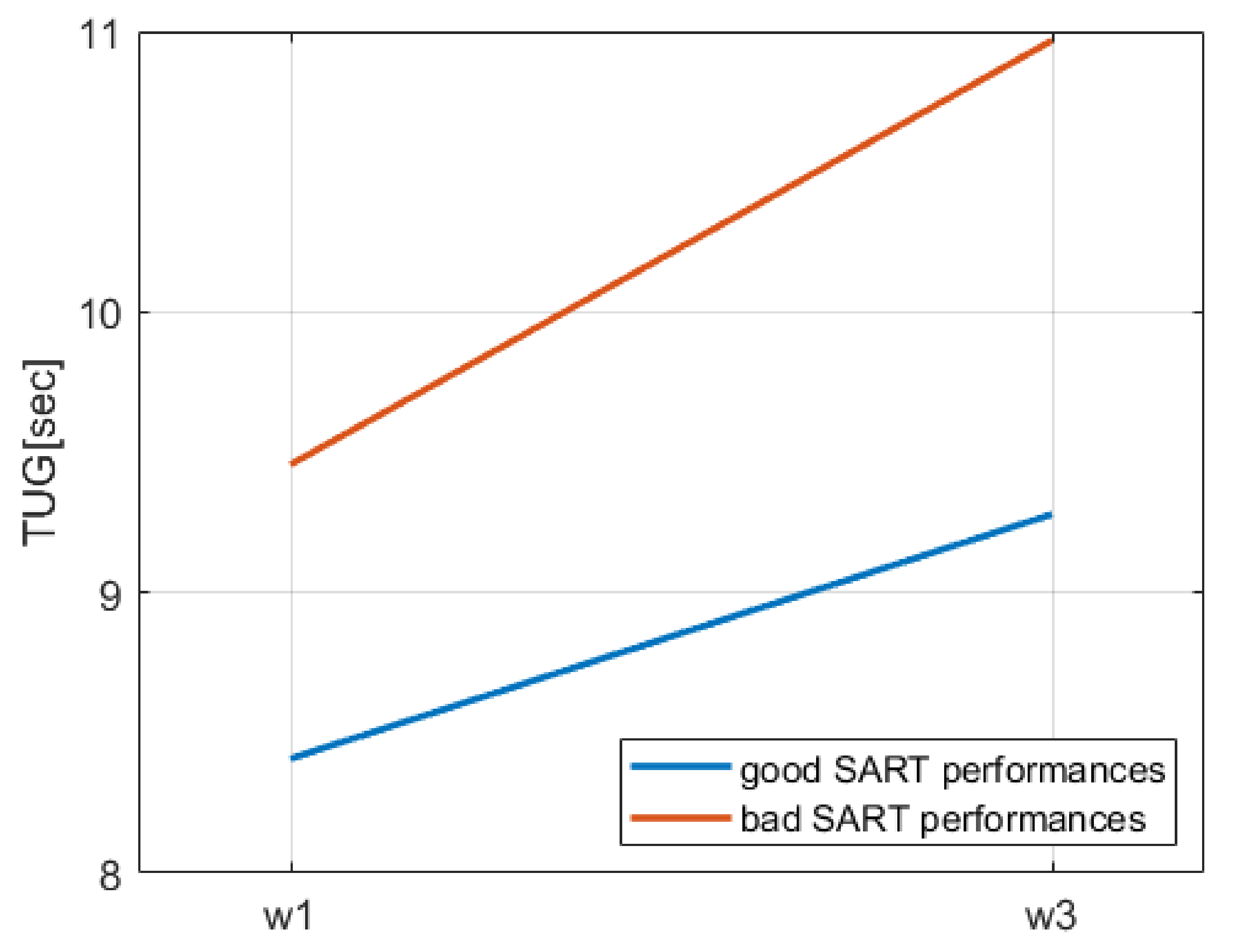
bad performances was a significant predictor of
TUG decline in the employed binary logistic regression models, being associated with an increase per unit of around 30% in the odds of having TUG decline in the fully adjusted models. Moreover, and consistently with previous literature on cardiovascular burden and mobility limitations in older adults [
63], we noted that in model 4, advancing age, the presence of antihypertensives and diabetes, and current smoking status were significant positive predictors of
TUG decline, bringing an increase in the probability for the outcome of about 14%, 94%, 68%, and 79%, respectively. Moreover, in keeping with the literature [
64] and clinical expectation, a significant negative predictor of
TUG decline was a high level of self-reported physical activity, which decreased by 32% the probability of
TUG decline. However, considering also UGS at baseline as a covariate in model 4a we noted that some independent variables lost significance in the prediction of
TUG decline; the only significant positive predictors were
bad performances, advancing age, and antihypertensive medication use, which determined an increase of 30%, 10%, and 67%, respectively, on the probability of the outcome, while higher UGS at wave 1 was protective against
TUG decline, leading to a decrease of 6% in the probability. We note that the difference of results between models 4 and 4a were probably due to the high correlation between
and
, and between
and
(Spearman’s correlation coefficient
at the significance level of 0.01). Therefore, it was highly probable that UGS at baseline would influence the probability of having a TUG decline after 4 years. Nevertheless, we note that even considering a variable strongly associated with the outcome,
bad performances did not lose its significance, demonstrating it to be a robust predictor of
TUG decline.
Our findings suggested that participants with SART bad performances and with a normal TUG at wave 1 ( s) had a 30% greater probability to have a TUG at wave 3 indicating a mobility impairment (i.e., s). Moreover, comparing the contribution of bad performances in the five models employed, we noticed that (i) even adding covariates, it remained a significant predictor, suggesting its robustness in the prediction of the outcome, and (ii) although its OR decreased in models 2 and 3 compared to model 1, it increased again in model 4, and even more in model 4a. The latter observation suggests that in models 2 and 3, other covariates significantly influenced the probability of the outcome, however these variables were not robust for the model, since the presence of further covariates in model 4 and 4a made their presence not significant for the model. In this case, bad performances remained significant and regained part of the prediction power temporarily lost in model 3. Furthermore, considering model 4a, where a variable (UGS) highly correlated to the outcome was used as a covariate, bad performances not only did not lose significance, but also its prediction power increased further, taking part of the weight from less robust independent variables, which were significant predictors in model 4.
Equivalently, we employed the first four logistic regression models for the prediction of
UGS decline. In this case,
bad performances was a significant predictor only in model 1, but was not significant in the fully adjusted model. To explain the difference in the results between
TUG decline and
UGS decline, we need to understand how these two mobility measures were taken. To measure UGS, participants were required to simply walk in a straight line. This task, then, does not require any major cognitive involvement, since walking is an action that is normally executed automatically in independent adults. Differently, TUG task requires participants to stand up, walk in a straight line, come back, and sit again. Thus, this test is more cognitively involved than straight-line walking, as the individual needs to process and remember instructions, plan and execute movements, focus on the task, and avoid distractions [
20]. SART
bad performances could capture cognitive processes that are similar to those required for completion of the TUG, and this could be a possible explanation as to why
bad performances independently predicted future mobility decline in our analyses.
Similarly, we considered SART bad performances as one of the independent variables in binary logistic regression models for the prediction of becoming a new faller at wave 3. We found that our new variable was a significant positive predictor in the fully adjusted models. In fact, the presence of SART bad performances in participants who did not have any falls at wave 1 contributed to an 11% additional probability of falls at wave 3, compared to those who did not have any SART bad performances at wave 1, i.e., who never hit the threshold of 4 mistakes in one trial. We noted that among all the other covariates used in the model, only age was a significant predictor of becoming a new faller at wave 3, although with a low positive contribution of only 2% to the odds of the outcome. Even in this case, comparing the bad performances contribution in the five models employed, we observed a phenomenon similar to that for the prediction of TUG decline. Indeed, we could notice a decrease in its prediction power in models 2 and 3 with additional loss of significance in model 3 due to the presence of significant predictors among the added covariates. However, in model 4 and 4a it reacquired significance and predictive weight, suggesting the non-robustness of previously significant covariates.
Comparison with Traditional SART Measures as Predictors
Traditional SART variables measure global features, such as the total number of mistakes (omission and/or commission errors) in the whole task, and the mean RT and SD RT across the whole task [
5,
17,
20,
24,
44]. However, using global parameters, which average a large complex dataset, such as the SART, important information residing in individual trials in the set of repeated measures may be lost. Indeed, no significant associations between SART global parameters and mobility status had been previously found [
17,
24]; and even when correlations involving reaction time measures had been found, the statistical effect was quite small [
25].
In the present study, we aimed to define a new variable, which, being more selective, could discriminate the participants with greater risk of mobility decline. We demonstrated that our variable bad performances was a significant predictor of risk of TUG decline and becoming a new faller. Furthermore, we compared its predictive power with other potential predictors: the global parameter total mistakes and mistakes in good performances, obtained by summing up all the mistakes in SART good performances, i.e., where the maximum number of mistakes per trial was less than 4. We noted that the variables bad performances and mistakes in good performances were almost complementary, because mistakes in good performances considers all the mistakes that are not reaching the threshold for the definition of a bad performance.
In the literature, there is not a uniform consensus on the method to follow in order to compare the importance of different predictors in binary logistic regression [
21,
65,
66]. We compared the models with the different potential predictors for
TUG decline,
UGS decline, and
new fallers considering the OR with non-overlapping 95% C.I. when the independent variable was significant for the prediction of the outcome.
In the fully adjusted models for the prediction of TUG decline, we found that, although all three variables considered were significant as predictors, the new variable bad performances had a higher OR compared to total mistakes and mistakes in good performances, where the difference between ORs considering the C.I. was equal or greater than 0.092 in model 4, and 0.083 in model 4a. Specifically, while the effect of the variable bad performances per unit was around 30% on the probability of the outcome, total mistakes, and mistakes in good performances had an effect per unit of only 3% on the probability of the outcome, namely 1 magnitude less than bad performances.
Regarding the prediction of UGS decline, no SART-related variables were significant as predictors for the outcome in the fully adjusted model. Bad performances, total mistakes, and mistakes in good performances were all significant in model 1, where bad performances assumed the highest OR, and total mistakes and mistakes in good performances were also significant in model 2, but they all lost their significance in models adjusted for covariates. This result may be due to the fact that, while UGS is a simpler measure of physical mobility, the TUG task is more cognitively involved and, thus, logistic regression models were able to detect the correlation with SART variables.
Moreover, we found that bad performances significantly predicted new falls, i.e., falls at wave 3 for participants who did not have any falls at wave 1, while total mistakes and mistakes in good performances were not significant predictors. Namely, our findings suggested that for participants who did not report any falls at wave 1, the number of mistakes in SART task was not a risk of falls at wave 3, as long as they did not hit the threshold of 4 mistakes in a single trial.
Furthermore, comparing the three predictors’ performance across the five models employed, we noticed that in the prediction of both TUG decline and risk of becoming a new faller, the predictors’ total mistakes and mistakes in good performances did not manifest the same phenomenon observed for bad performances. Namely, the presence of covariates in models 2 and 3 was associated with a decrease in prediction power, expressed by the OR, of total mistakes and mistakes in good performances for both outcomes, with additional loss of significance in model 3 for total mistakes and models 2 and 3 for mistakes in good performances in the prediction of new fallers. Differently from the models involving bad performances, in this case in model 4 and 4a the predictors did not reacquire prediction power nor significance for the prediction of new fallers, suggesting that they were not robust and strong enough in the prediction, and possibly other covariates revealed to be significant in the model.
Our results suggest that when SART mistakes reach threshold status, the number of times that this happens should be taken seriously as potentially heralding mobility decline and/or falls; however, mistakes below threshold level were less predictive and this could be used to reassure participants that ‘one swallow does not make a spring’ when it comes to interpreting the clinical significance of a participant making sub-threshold mistakes during the SART task. This still agrees with the principle that clinicians who administer tests of neurocognitive performance (such as the SART) should be reluctant to attribute poor test performance to anxiety that occurs during the testing process [
67], but at the same time argues in favour of not placing undue emphasis on the clinical significance of mistakes that occur below a proven threshold. Interestingly, anxiety was not a significant covariate in any of the fully adjusted logistic regression models, which further dilutes the potential mechanistic role of anxiety in the prediction of the four clinical outcomes under study. Another interesting insight from our analyses is that once the focus was on the new visualisation features and additional covariates, mean SART RT and SD of RT had no independent effect on the prediction of any of the outcomes. Since RT variables have been the main focus of previous research on SART-related health outcomes, we would support the need to revisit those studies fort the potential effects of thresholded error features as reported herein.


 ,
, 


