Bonding States of Hydrogen in Plasma-Deposited Hydrocarbon Films


Max-Planck-Institut für Plasmaphysik, Boltzmannstr. 2, D-85748 Garching, Germany
*
Author to whom correspondence should be addressed.
C 2020, 6(1), 3; https://0-doi-org.brum.beds.ac.uk/10.3390/c6010003
Submission received: 28 October 2019
/
Revised: 13 December 2019
/
Accepted: 20 December 2019
/
Published: 9 January 2020
(This article belongs to the Special Issue Characterization of Disorder in Carbons)
Abstract
:We applied temperature-programmed desorption (TPD) spectroscopy to study the bonding of hydrogen in amorphous hydrogenated carbon (a–C:H) films. Typical hard plasma-deposited a–C:H films with an initial hydrogen content (H/(H+C)) of about 30% were used as samples. About 85% of the initial hydrogen content is released in the form of H2, the rest in the form of hydrocarbons. Using a temperature ramp of 15 K/min, release of hydrogen starts at about 600 K with a first peak at about 875 K and a broad shoulder around 1050 K. The peak positions depend on the temperature ramp. This fact was exploited to determine the pre-exponential factor for an analytic analysis of the release spectra. This analysis revealed a pre-exponential factor of 1/s, which deviates significantly from the frequently assumed prefactor 1/s. This higher prefactor leads to a shift in the determined binding energies by about +0.5 eV. Standard TPD measurements with linear temperature ramps up to 1275 K were complemented by so-called “ramp and hold” experiments with linear ramps up to certain intermediate temperatures and holding the samples for different times at these temperatures. Such experiments provide valuable additional data for investigation of the thermal behavior of the investigated films. Our experiments prove that the width of the hydrogen release spectrum is determined by a distribution of binding energies rather than release kinetics or diffusive effects. This binding energy distribution has a peak at about 3.1 eV and a shoulder at higher energies extending from about 3.6 to 3.9 eV.
Keywords:
thermal desorption spectroscopy; amorphous hydrocarbon film; inverse problem; Bayesian inferencePACS:
68.60.Dv; 81.70.Pg; 68.55.-a; 28.52.Fa1. Introduction
Amorphous hydrogenated carbon (a–C:H) films have a number of very interesting physical and chemical properties [1,2], which make them possible candidates for a wide range of technical applications. Discussed applications include optical, mechanical, electronic and biomedical applications [3]. Examples are protective coatings on devices such as hard disks [4,5,6], diesel-injection systems [7] and coronary stents [8,9] or other medical applications [10]. A significant number of such technical applications is based upon the outstanding tribological properties of a–C:H films [5,11,12,13] and for many technical applications the thermal stability of a material is a topic of relevance. First systematic investigations of the thermal decomposition of a–C:H films were published by Wild and Koidl in 1987 [14]. Later on, thermal release of hydrogen from hydrogen containing carbon films or thermal decomposition of such layers has gained some attention in the field of thermonuclear fusion [15,16,17,18,19,20,21,22] and due to this the thermally induced release of hydrogen was studied to some extend in dedicated laboratory experiments. Küppers and co-workers [15,23,24,25] investigated this topic in the early nineties. They used thin ion-beam deposited films with thicknesses ranging from one to ten monolayers and investigated them in an ultrahigh vacuum system using thermal desorption spectroscopy and high resolution electron energy loss spectroscopy. Their results will be discussed in detail in Section 5.
Salançon et al. have published two articles regarding the thermal decomposition of plasma-deposited a–C:H films [26,27] which concentrated on polymer-like, hydrogen-rich, soft a–C:H films. Thermal decomposition of these films produces a vast variety of hydrocarbon species with significant contributions of CxHy species containing up to five carbon atoms and even traces of molecules with up to seven carbon atoms were detected. Comparing the thermal decomposition of soft, hydrogen-rich films with that of typical hard a–C:H films they found that the relative contribution of high molecular weight species is much higher for soft films compared with hard films. This is in agreement with published results for a-C:H films [14,28,29,30] and it is a consequence of the difference in microstructure of the films. While the hydrogen in hard a–C:H films is dominantly released in form of H2, release from the soft films is dominated by hydrogen bonded in hydrocarbon species. These hydrogen-rich soft films possess not only a different spectrum of released species but release occurs also at much lower temperatures [27].
Thermal release spectra of D from different D-containing carbon layers were also analysed by Pisarev et al. [31]. The D release spectra of typical hard a-C:H films shown in [31] are, in principle, nicely comparable with those by Salançon et al. A remarkably comprehensive characterisation of annealing-induced changes of the many different properties of various plasma-deposited a–C:H films was published by Peter et al. [32,33]. Overall, their findings regarding thermal stability are also in good agreement with the earlier studies. However, an advanced evaluation of the thermal release data (e.g., determining binding energies) was not made in both cases.
This article is focussed on the thermally induced release of hydrogen from hard a–C:H films. Previous investigations have shown a rather broad release spectrum ranging from about 600–1250 K. Questions to be addressed are: How is hydrogen bonded in a–C:H films? Is the observed peak width mainly due to the release kinetics (bond breaking, diffusion and desorption) or a consequence of a distribution of binding energies? We performed dedicated experiments to address these questions.
One remark regarding nomenclature: In the literature, different names are used for the method we apply here: thermal desorption spectroscopy (TDS), temperature-programmed desorption (TPD), and thermal effusion spectroscopy (TES). These different names emphasise different aspects of the underlying process. We do not want to argue about the pros and cons of these names here. We just state that, although we used TES in the past (and that is the reason for naming our experimental setup), we are going to use temperature-programmed desorption (TPD) throughout this article.
2. Experimental
2.1. TESS
The experiments were carried out in the device TESS (Thermal Effusion Spectroscopy Setup). The configuration and possibilities of TESS were described in detail in Ref. [27]. In short: TESS is an ultrahigh vacuum (UHV) experiment equipped with a cryopump (Cryo-Torr 8, CTI cryogenics) to provide high pumping speed (pumping speed for H2: 2500 L/s) and a sensitive quadrupole mass spectrometer (QMS), both located in the main stainless steel chamber. In contrast to the configuration described in Ref. [27], the liquid nitrogen trap in the main chamber was removed and replaced by two pumps in series (classical turbo Leybold 1000C with 970 L/s H2 pumping speed backed with a Pfeiffer TMU 071 turbo drag pump with high compression ratio for hydrogen). This provides an even higher total pumping speed compared with the earlier configuration and allows in addition investigations including helium, which is not efficiently pumped by the cryopump. The base pressure of TESS is in the 10−8 Pa range.
The quadrupole mass spectrometer is a Pfeiffer/Inficon DMM 422 equipped with a cross-beam ion source and a sensitive secondary electron multiplier that was operated in ion counting mode. All experiments were conducted with an electron energy of 70 eV. The emission current was set to 0.6 mA.
For all measurements presented here, only the remote UHV oven of TESS was used. This oven consists of a long quartz glass tube inserted into an external tubular oven. The heated volume of the oven is 4 cm in diameter and 40 cm in length. The external oven is mounted on a rail system. It can be moved over the entire length of the quartz tube and can even be removed completely from it. The length of this quartz glass tube is 45 cm and its inner diameter is 2.2 cm (outer diam. = 2.54 cm). The glass tube is connected to the main chamber via a gate valve.
Samples are loaded by removing the tube and placing several samples in the glass tube. After mounting the glass tube back to the vacuum system, it is pumped via a second gate valve through the load lock to a sufficiently low pressure (better than 10 Pa, base pressure = 10 Pa). For measuring effusion spectra the gate valve to the main chamber is opened. The background pressure in the main chamber during a measurement with the oven setup is in general Pa. A sketch of the experimental setup can be found in Ref. [27]. We only add here the actual dimensions used in the present study. Samples are stored at one end of the glass tube close to the gate valve to the main chamber. The measurement position is about 40 cm away from this position (5 cm from the other end of the tube). The external oven is movable and during the measurement centered around the sample location. The oven size defines then the distance of the samples in the storage position from the end of the hot zone to about 15–20 cm. Samples can be moved inside the glass tube without breaking the vacuum from the storage position to the measurement position. This is done indirectly via a piece of nickel inside the tube that can be manipulated by a small magnet from outside thereby pushing samples back and forth when the oven is retracted and the tube is cooled down. This procedure allows to minimize gas desorption in two ways: First, the glass tube can be cleaned up to the highest temperature later used in the temperature ramp and second we do not need a target holder that could potentially outgas during the ramp. The disadvantage of this design is that the sample temperature can only be derived by calibration measurements after the ramps with a dedicated sample with a thermocouple attached to it.
Prior to an experimental campaign in the oven, the measurement region is heated to 1300 K for one hour to thoroughly clean the glass tube and to reduce background contributions from the walls of the glass tube during the measurement. The sample is transferred from the storage position to the measurement position after tube and oven have cooled to about room temperature. Then the measurement is immediately started. Species released in this quartz glass oven reach the ionizer of the QMS only after many collisions with the walls of the quartz tube and the main vacuum chamber, so that reactive species which are lost in wall collisions cannot reach the ionizer (see [27]). With this setup only stable, non-reactive species can be detected. In this article, we are only concerned with the stable species H2 and CH4, thus redeposition on the chamber walls plays no role. Also, based on findings in [27] the formation of stable species on the chamber walls after release of reactive species is assumed to be negligible for the kind of films investigated here.
2.2. Temperature Calibration
The temperature of the oven was measured by an insulated metal sheathed thermocouple (type K, chromel-alumel) fixed close to the inner wall of the oven facing the glass tube and recorded in the data file together with the experimental data. The signal from this thermocouple was used to feedback control the oven temperature by a temperature controller (Eurotherm 902P). The oven can provide heating rates of up to 40 K/min. The true sample temperature is lower than the measured oven temperature and had to be determined in separate calibration measurements for each individual ramp. For these calibration measurements a thermocouple (chromel-alumel, 0.125 mm) was fixed to a test sample which was placed at the sample position inside the quartz glass tube. Two effects have to be considered: (i) although the sample is in the radiation field of the external oven, the steady-state temperature of the sample is somewhat lower than the oven temperature. (ii) during temperature ramps the sample temperature always lags behind the oven temperature. The sample temperature depends on several factors: the actual heating rate, the reflection coefficient and the thermal capacity of the sample. All samples used in the present study were a–C:H coated single crystalline silicon samples cut from the identical wafer. This assures that the sample properties are identical in all experiments. Test experiments have shown that, e.g., the sample temperature of tungsten samples differs significantly from that of our silicon samples. We carefully measured calibration curves for the sample temperature as a function of the oven temperature for all used heating rates. The reproducibility is in general excellent, and the uncertainty of the temperature determination for the here investigated samples is estimated to ±5 K.
Results of the temperature calibration measurements are shown in Figure 1. The figure shows the oven and the corresponding sample temperatures on a normalized time scale. The time scale was normalized such that the oven temperatures for the different used temperature ramps coincide. This means that for example the time scale for the 3 K/min temperature ramp is compressed by a factor of 5 compared with the 15 K/min ramp. All sample temperature ramps exhibit a similar behaviour. At low oven temperature the sample temperature shows a significant lag compared with the oven temperature. This temperature lag increases strongly with increasing heating rate. For oven temperatures in the range of 350–400 K the samples start to heat up and pass into a mostly linear ramp for T above about 600 K. In the sample temperature range from 600 K to the maximum temperature the deviation from a linear behaviour is small for nominal ramps of 3 up to 15 K/min, but the ramps with 30 and 40 K/min show significant deviations for T above about 1000 K. At the end of the oven temperature ramp the sample temperature still increases for some time. The time lag until the steady-state temperature is reached depends also on the used temperature ramp. For the mostly used ramp of 15 K/min it takes about 5 min. For the experiments presented in this article the maximum oven temperature was 1275 K. The corresponding steady-state sample temperature is 1198 K. The desorption peaks we are interested in occur in the temperature range from 800 to 1000 K and are thus located in the mostly linear part of the sample temperature ramp. The true sample temperature ramps are given in Table 1. They were determined from the slope of the ramp at the position of the first desorption peak. The reason for this choice will become clear in Section 3 in the analysis according to Equation (7). We want to point out that the linearized average rate in the range from 800 to 1000 K deviates less than 2% from the values given in Table 1. For simplicity, we will use in the remainder of this article the oven temperature ramps to identify different experiments and call them nominal temperature ramps.
2.3. Layers
Amorphous hydrogenated carbon films (a–C:H) were produced in an asymmetric capacitively coupled RF plasma setup using methane (CH4) as working gas. The plasma chamber consists of a stainless steel vessel and was pumped to a base pressure in the 10 Pa range by a turbomolecular pump. Prior to deposition the substrate surfaces were cleaned by sputtering in an oxygen plasma followed by a hydrogen plasma (bias voltage −300 V, 30 min each). The total methane (CH4) pressure is kept at 2 Pa and the gas flow is adjusted by a mass flow controller at 20 sccm (standard cubic centimeters per minute). To deposit hard a-C:H films the silicon substrate was placed on the driven RF electrode which, reached a self-bias voltage of −300 V. Typical hard, so-called diamond-like amorphous carbon films with a hydrogen content of H/(H+C) ≈ 0.3 are produced under such conditions [34,35]. The used layers have a refractive index of = 2.16 − i 0.1 at 632.8 nm and a thickness of 89 nm as determined by ellipsometry. The deposition of this layer takes about 14 min. Other physical parameters of comparable layers can be found in Ref. [35]. Films were deposited on silicon wafers 100 mm in diameter and 300 μm in thickness. The film homogeneity across the wafer is better than 5% as measured by ex-situ ellipsometry. All samples used for thermal effusion measurements had the identical size of 10 mm by 10 mm (= coated area) and were cut from the identical wafer. This assures that the samples used in the different experiments are absolutely comparable in terms of absolute quantities. After film deposition the samples are exposed to ambient atmosphere. Hard a-C:H films are long-term stable. Neither TPD measurements nor ion beam analyses have shown a significant uptake of water.
2.4. Experimental Procedures
Temperature-programmed desorption (TPD) spectra were recorded in two complementary modes. In a normal TPD run, the temperature is ramped up from about room temperature to the maximum temperature with a linear temperature ramp. The maximum temperature for all normal runs was set to 1275 K. During the temperature ramp predefined mass channels as well as oven temperature and total chamber pressure were recorded as a function of time. Typically up to 29 mass channels were recorded quasi-simultaneously in the so-called “multiple ion detection mode”. A dwell time of 0.5 s for each mass channel was chosen. In this article we present almost exclusively data for the 2 amu signal. With the temperature calibration discussed in Section 2.2 these data can be plotted also a function of sample temperature (see Figure 2). The 2 amu signal is fully attributed to the release of molecular hydrogen. In Figure 2b, only one desorption spectrum for 16 amu (dominantly due to CH4) is shown for comparison. More information on the product spectrum of different a–C:H films can be found in Refs. [26,27].
Figure 2 shows a typical result for a normal TPD run. In Figure 2a the QMS signal is plotted as a function of time. The nominal temperature ramp for this experiment was 15 K/min. Such a measurement takes about 66 min (1000 K/15 K/min). For comparison, to cool down the oven to about 300 K after an experiment lasts about 2 h. The black, open squares in Figure 2a are the raw QMS signal. Also plotted in this figure are the oven and sample temperatures (solid lines). After stopping the oven ramp at 1275 K the sample temperature is still increasing for about five more minutes as discussed in detail in Section 2.2. Also shown in Figure 2a is the background signal measured on mass channel 2 amu for an empty glass tube (red, open circles). The background signal is constant from room temperature to about 1100 K, then it starts to increase. This increase is due to release of hydrogen from the quartz glass. The magnitude of the increase depends to some extent on the history of the tube, in particular on the maximum temperature reached in the preceding TPD run. For the set of experiments discussed in this article, the background turned out to be very reproducible. This background signal was subtracted from the raw QMS data to yield the background subtracted data (blue, solid squares). The background subtracted data are shown again in Figure 2b as a function of sample temperature. In addition, the 16 amu signal is shown for comparison. The results shown in Figure 2 will be discussed in detail in Section 4.
In the second measurement mode, samples are heated up to a certain temperature, Thold, then heating is stopped (temperature ramp 1) and the sample is held at that temperature for a certain time, thold. Then the oven is removed from the sample, which causes a fast cool down to room temperature. After the external oven has also cooled down to about 300 K (this lasts about 2 h) the oven is again moved over the glass tube and a second TPD run, now up to the maximum temperature, is started (temperature ramp 2). A schematic temperature characteristic of such an experiment is shown in Figure 3. We call these types of experiments “Ramp and Hold” (R&H) experiments. Measurement parameters for such R&H experiments are: the “holding temperature” Thold and the “holding time” thold. All R&H experiments presented here were recorded with a nominal oven temperature ramp of 15 K/min.
3. Theory
Thermal desorption of adsorbed or chemisorbed species is commonly studied within the framework of transition-state theory [36,37], resulting in the familiar expression
for a first-order desorption process with a single activation energy . Here, is the total number of released species per time and is the corresponding population at time t of sites with activation energy and the pre-exponential factor is a rate constant. k denotes the Boltzmann constant. If the temperature T is increased as function of time with a linear rate
then Equation (1) can be solved analytically for . The initial condition yields a solution in terms of exponential integrals and double exponentials
with being defined as:
Equation (3) holds also for ratios, where the second order Taylor expansion of Redhead [38] becomes inaccurate. The key parameters of Equation (1) are the pre-exponential factor and the activation energy which will be considered in the following. In principle, also a second-order process like H+H → H2 could appear to be a reasonable assumption for the rate-determining step. However, none of the characteristic features of a second order process are present in the TPD spectra: neither left-right symmetric peaks nor the characteristic temperature shift of the peak position as a function of the population. Thus we used a first-order process only. Also the analysis of TPD data of carbon films deposited in tokamaks supports the presence of a first order process in the release of hydrogen [39]. Furthermore, it has been shown [40] for hydrogen implanted graphite that molecules during thermal desorption form locally, i.e., at the location where the (first) C-H bond breaking process occurs.
3.1. The Pre-Exponential Factor
The thermally activated escape rate of a particle from a metastable state A through a transition state TS can be estimated by [41]
where and represent the partition functions in the metastable well and at the transition state, respectively. h is the Planck constant. Depending on the available degrees of freedom gained by the particle leaving the metastable state very large pre-exponential factors (exceeding 1/s) may occur [42]. Therefore, although the desorption function is not very sensitive to variations in the pre-exponential factor a simple (but common) assignment of a typical vibration frequency as attempt frequency for the pre-exponential factor (e.g., 1/s) may result in wrong or biased conclusions (c.f. remarks and recalculations in [43]). For the hydrocarbon films and process considered here the metastable well corresponds to a hydrogen atom bonded to a carbon atom and the transition state to the moment of C-H bond breaking. In comparison to a hydrogen in a C-H bond the non-bonded hydrogen atom is relatively unconstrained—thus a prerequisite for large pre-exponential factors is present. In the present experiment the pre-exponential factor was determined from a series of measurements with different temperature ramps . For a single activation energy the temperature at which the desorption rate is at maximum is given by the solution of
which can be expressed as (see e.g., [44])
For a first order desorption the plot of against for different temperature ramps should give a straight line with slope and the pre-exponential factor can be obtained from the intercept with the y axis.
3.2. The Population Density as Function of Energy
The deposited hydrocarbon films are known to be amorphous. Therefore, a single or even a set of well-defined activation energies is not to be expected—instead a continuum of activation energies is more likely. Then the desorption is given by
using the generalization of to a energy-dependent population density with initial population . If the release processes are independent, then the time dependence of the population is given by Equation (3) for each energy E. However, this holds only if other transport processes (i.e., diffusion) have negligible impact and has to be confirmed by an independent measurement. This is most easily achieved by varying the thickness of the investigated layer (c.f. Section 4).
3.3. Bayesian Data Analysis
The conventional way of assigning numerical values to the model parameters is to perform a ‘least squares fit’. By doing so, one ignores that in general expert knowledge exists, e.g., that the population density has to be non-negative. From simply fitting the model to the data by maximizing the likelihood, it may happen that ‘best fit parameters’ assume negative values. In that case expert knowledge is commonly applied in a destructive way—the fitting result is rejected as being unphysical. Within the Bayesian approach [45] the available expert knowledge enters the analysis as prior probability distribution for the parameters . In the present notation (following [45]) expresses the conditional probability (density) for A given that B is true. The symbol I denotes all the background information which is implicitly used or available but at present is not at the center of interest. The prior distribution affects the posterior distribution (the probability distribution for the parameters given the observed data D) through Bayes’ theorem
essentially by multiplication of the likelihood with the corresponding prior probability for . The likelihood term describes the probability to observe the data D given that the parameters are . The posterior distribution is normalized to one by the term in the denominator, the so-called evidence . Although this term is important for model comparison applications [46] for the present manuscript it acts as a proportionality constant Z only. Once the posterior distribution for the parameters is available summarising quantities like mean or variances can be assessed easily, e.g.,
Excellent introductions to Bayesian probability theory are available (see, e.g., [45,46]) and applications of Bayesian probability theory to a variety of physical problems are summarized, e.g., in [47]. In the present application, the prior for the population density is chosen to be constant for some range of binding energies and zero outside:
thus restraining the solution space to physical reasonable solutions while otherwise coinciding with a standard maximum-likelihood approach. The choice of and is discussed in Section 3.3.2.
3.3.1. The Likelihood Distribution
The combined evaluation of different TPD measurements requires a careful quantitative description of the measurement uncertainties of the individual TPD profiles. For counting experiments with mean the likelihood for the signal (counts) is given by a Poisson distribution
The number of counts have been obtained by multiplying the instrumental output (given in units of counts/second) by the actual integration (dwell) time : the uncertainty of the normalized data in counts/second for different measurement times do not follow a common probability distribution and are therefore not advantageous as basis of a joint likelihood distribution.
For a sufficiently large number of counts () the Poisson distribution can be approximated by a Gaussian distribution with standard deviation .
Subtracting the intensity of the corresponding background measurement yields and increases the uncertainty of data to
resulting in the likelihood distribution
The model function for this data point is given by the time integration over the desorption rate (c.f. Equation (8))
thus describing the expected number of particles being desorbed in the time interval for a heating rate of and a population density . From Equation (14) for a single data point we can now construct the likelihood function for a TPD profile :
The posterior distribution of the population density—eventually combining a set of K different TPD measurements employing different heating schemes and holding times—can then be written as
where Z denotes the normalization constant. Please note that all measurements are combined to estimate a single initial population density. Although the time evolution is deterministic once the temperature is known as function of time, a variation of the heating scenarios can result in a very different evolution of the population density, which in turn constrains the initial distribution.
3.3.2. Algorithmic Details
One of the crucial parameters in the calculation of TPD profiles is the heating rate , which is in general a function of temperature . The local heating rate has been determined from the temperature measurements by first fitting a cubic regression spline to the temperature data [48], followed by analytic differentiation at the measurement times to obtain . In this way the roughening effect of a finite difference approach is circumvented [49].
The total number of particles
available for desorption is the same for all simulated TPD spectra. However, the integrated yields of the experimental TPD spectra exhibit small fluctuations (less than ), which are likely to be due to fluctuations in the sample area. To compensate for this fluctuations all experimental data are normalized to the same integral yield and the data uncertainty is correspondingly adjusted.
The population density estimation is done numerically with a Monte Carlo Markov Chain (MCMC) computer code [50,51,52] using a non-parametric approach. Within the limits of a vector of L support points and a corresponding vector of population densities are randomly and independently chosen (obeying the detailed balance condition). Then a piece-wise linear interpolation of the support points is used as proposal for the population density and accepted/rejected according to the standard Metropolis–Hastings algorithm. The edge points of the population density are kept constant: because there are no indications of any measurable population at lower binding energies in the experimental data. It should be noted that on highly oriented pyrolithic graphite (HOPG) surfaces hydrogen binding energies of around 1.5 eV have been derived [53] but the present measurements do not exhibit any of the corresponding low-temperature desorption peaks at sample temperatures below 500 K. This is supported also by calculations using a lower limit of eV which resulted in negligible populations for binding energies below 2 eV. The high energy edge is also set to zero, because a population above 5 eV would not contribute to the TPD signal for the upper temperature limit used in this study. This is supported by ion beam measurements after the TPD experiments where the remaining hydrogen amount is less than 5% of the initial amount (see Section 4). Binding energies of almost 7 eV as reported in [54] will, therefore, even if present, not affect the results.
The number of support points has been chosen in such a way that the average of the fitted spectra fulfills the classical condition with denoting the number of used data. Fitting attempts with a smaller number of support points exhibit a drastic increase of the values indicating that then the population density is not flexible enough to accommodate the measured data. On the other hand, a further increase of the number of support points has a negligible effect on the quality of the fit. This indicates that the eventually chosen number of 8 support points is sufficient for a reasonable fit but without being prone to overfitting. Profiles with nine or ten support points yield virtually identical density estimates. The profile is computed using the standard technique of weighted averaging of the individual MCMC samples. To minimize correlation effects only every 100th sample was used for the computation of the average. It should be pointed out that also other approaches of estimating a density function exist (see, e.g., [55,56,57]), but that in all cases considerable computational effort is mandatory.
4. Results
Most experiments were performed for a nominal temperature ramp of 15 K/min. The calibration experiments have shown that for this ramp the sample temperature follows closely the oven temperature and that the sample temperature slope is linear over a wide range. This ramp is a good compromise between linearity of the ramp, signal intensity, and required time for one experiment. Figure 2 shows a typical TPD spectrum for a hard a–C:H film. The data processing presented in Figure 2a was discussed in Section 2.4. The processed data are shown in Figure 2b as a function of sample temperature. No significant H2 desorption is found for temperatures lower than 600 K. With further increasing temperature the signal increases strongly and reaches a maximum at 875 K (1st peak). For higher temperature the signal decreases and shows a shoulder in the range of 1000–1100 K (2nd peak). We assign a temperature of approximately 1050 K for the second peak. For temperatures larger than 1100 K the signal decreases further. However, when the maximum oven temperature of 1275 K is reached the signal has not yet gone to zero. This is certainly an unsatisfactory situation, but higher sample temperatures were not possible in the present set of experiments. After such a TPD experiment up to an oven temperature of 1275 K about 5% of the initial amount of hydrogen remains in the sample. This was checked by ex-situ ion-beam analyses of samples after TPD experiments [58]. This retention of a small amount of the initial hydrogen content does not influence the conclusions for the temperatures below 1170 K. We further emphasize that the TPD spectra for different individual samples show excellent reproducibility. Also presented in Figure 2b is the TPD signal for 16 amu, which is predominantly due to methane. The methane peak occurs at approximately the same temperature as the first hydrogen peak but falls off quickly at higher temperatures reaching background level at about 1000 K. We have shown earlier [27] that the hydrogen release is accompanied by release of various hydrocarbons. For hard a–C:H films the release of hydrogen containing volatile species is by far dominated by molecular hydrogen. Quantitative analyses of the QMS spectra have shown that about 85% of the hydrogen in the hard a–C:H film is released in form of H2 [58]. The contribution of CxHy is however not topic of this article and the interested reader is referred to Ref. [27] for further discussion.
Figure 4 presents two examples of R&H experiments for Thold = 878 K. The data in Figure 4a are for a holding time of 0 min, i.e., the oven was immediately removed from the glass tube after reaching the oven target temperature of 917 K (this corresponds to a momentary sample temperature of 845 K). Figure 4b presents equivalent data for a holding time of 60 min. In this experiment the oven was kept at the target temperature of 917 K for 60 min and then removed. This oven temperature of 917 K corresponds to a steady-state sample temperature of 878 K. However, due to the time lag between oven and sample temperature as was described in detail in Section 2.2, the sample temperature increases for about another 5 min after the oven has reached the holding temperature. As a consequence, the maximum temperature for zero holding time is only 845 K. Both figures show the reference spectrum from Figure 2 for a continuous ramp up to the maximum temperature (black open squares) and the data for the first (red solid circles) and second (green solid circles) ramp of the R&H experiments. In both cases, the signal during the first ramp up to the holding temperature is practically identical to the reference spectrum. Removing the oven after reaching the target temperature (Figure 4a) leads to an almost instantaneous drop of the sample temperature and correspondingly to a drop of the 2 amu signal to background level. In Figure 4b, the 2 amu signal still increases a little bit after reaching the target temperature (this is due to the discussed time lag between sample and oven temperature) and then falls off rapidly.
The QMS signals of the two second ramps differ depending on the holding time spent at Thold. The spectrum during the second temperature ramp in Figure 4a (thold = 0 min) reproduces the part of the reference signal that is released at sample temperatures higher than the maximum temperature reached during the first ramp. The spectrum during the second temperature ramp in Figure 4b (thold = 60 min) shows only the second peak, but in both cases, the high temperature part of the TPD spectrum is unaffected. Holding the sample at 878 K for about 60 min is able to release some additional hydrogen compared with thold = 0 min, but it is not able to significantly depopulate the states at higher temperature (more than 150 K above Thold).
The whole set of R&H experiments at 878 K with varying holding time thold is presented in Figure 5. Figure 5a shows the QMS 2 amu signal recorded during the first ramp up to the oven temperature of 917 K and the corresponding sample temperature evolution. The increasing flanks of the first peak for the four different experiments are practically indistinguishable. Only the curve for a holding time of 0 min ends abruptly and has a slightly lower maximum value than the other shown curves. This is due to the temperature lag discussed above (see discussion of Figure 4). This temperature lag can be clearly seen from the sample temperature characteristic, which still increases for about five more minutes after the oven has reached its maximum temperature. The decaying part of the peak for the different holding times of 10, 30 and 60 min is also practically identical except for the fact that effusion stops abruptly after the different holding times. The peaks from the second ramp (Figure 5b) exhibit a continuous transition between the two cases shown in Figure 4. What is particularly remarkable is that the high temperature part of the different experiments is identical. Increasing holding time leads to increasing release of some additional hydrogen. States which would be released during a normal TPD run at slightly higher temperature than Thold are depopulated faster than higher lying states, but the high temperature part of the release spectrum is practically unaffected. In addition to the data shown, some experiments with different Thold were performed which show in principal identical behaviour. Also TPD measurements with samples exhibiting a layer thickness of 300 nm have been performed. Despite the significantly larger thickness (almost a factor of four), the TPD peak positions are not delayed.
This observation, together with the results presented in Figure 4 are a clear proof that the width of the TPD spectrum is not due to diffusive effects but represents the binding energy distribution (BED) of hydrogen in the a–C:H film. This will be discussed in more detail in Section 5. In the remainder of this article, we will use the phrase ‘binding energy distribution’ instead of ‘population density’, which was used in Section 3. While the latter is more appropriate in the theoretical description of the problem, we consider the former more suitable to convey the experimental findings. To reconstruct the BED from the experimental data, the pre-exponential factor for Equation (1) has to be determined. As discussed in Section 3 (see Equation (7)), can be determined from the shift of the TPD peak as a function of different temperature ramps. Figure 6 shows TPD spectra as a function of sample temperature measured for temperature ramps ranging from 3 to 40 K/min. Two facts are obvious: First, the height of the peak varies strongly and second, the position of the maximum shifts to higher temperatures with increasing heating rate. The shift of Tpeak is the effect that allows determining . The change in signal intensity is due to the change in release rate. Please note that for the different ramps, the different signal heights are expected because the total number of released species is constant rather than the release rate. We have checked that the time integral of the TPD spectra for the different ramps is in good agreement. In other words, the total amount of released hydrogen during these experiments with different temperature ramps is identical. The nominal oven temperature ramps, Roven, the corresponding sample temperature ramps, Rsample, and maximum peak temperatures, Tpeak, are given in Table 1. Due to the slight deviation of the true sample temperature ramp from linear behaviour as discussed in Section 2, the value for Rsample given in Table 1 is the derivative of Tsample at position Tpeak.
The left-hand side of Equation (7) is plotted in Figure 7 as a function of 1/Tpeak. The data lie on a straight line from which we determine 1/s. The uncertainty of the line fit results in lower and upper limits of the confidence interval of 1/s and 1/s, respectively. This range deviates significantly from the value of 1/s, which is usually assumed if nothing else is known [23,24,59]. The consequence of this much higher pre-exponential factor for the analysis will be discussed in Section 5.
Applying the experimentally determined pre-exponential factor all measured TPD spectra for 2 amu can be excellently fitted by one generic binding energy distribution. The different series of TPD spectra and the corresponding experimental parameters used to derive the BED are summarized in Table 2. The evaluation procedures were described in Section 3. In total, we used 11 independent experiments to derive the BED.
Figure 8 and Figure 9 show examples of a comparison between the measured data and the simulated data based on the generic BED. The overall agreement is excellent. Figure 8 shows three curves from the series with different temperature ramps. The symbols represent the data points and the solid lines the model results. The model can hardly be distinguished from the experimental data. In Figure 9 we plot two time traces of R&H experiments. In this plot the times scales of the first and second ramp are simply concatenated. The agreement between model and experimental data again is very good. Small deviations occur only at the tip of the first peak and around the maximum of the second peak. The comparison of the other 6 data sets used for deriving the BED with the model result is of equal quality to those shown in Figure 8 and Figure 9.
The generic binding energy distribution extracted from the data is presented in Figure 10. Hydrogen bonded in the investigated a–C:H films gives rise to a BED starting at about 2.5 eV and extending to about 4 eV. The shape is similar to the shape of the TPD spectra with a peak at around 3.2 eV followed by a broad shoulder extending to about 4 eV. A small pre-peak extends from about 2.5 to 3.0 eV. The confidence interval also shown in Figure 10 was derived according to the algorithm described in Section 3.
5. Discussion
First temperature programmed desorption measurements of plasma-deposited a–C:H films were published by Wild and Koidl in 1987 [14]. They have shown that the TPD spectra of different films change drastically with film structure. The effusion spectra for typical hard a–C:H films (in their case for deposition at bias voltages of 500 V and more) are in good agreement with our spectrum shown in Figure 2. They applied a heating rate of 20 K/min, which lies in the range of temperature ramps applied in our experiments (3–40 K/min, see Figure 6). In their case the first peak is located at 870 K and the second peak occurs at about 970 K. While the first peak is in very good agreement with our results of 875 K at 15 K/min and 891 K at 30 K/min, their second peak occurs at significantly lower temperature than ours (≈ 1050 K).
In the early nineties, Schenk and co-workers conducted a detailed study of the thermal decomposition of ultra thin a–C:H films [23,24,59]. They produced thin—of the order of 1 to 10 monolayers—films by ion beam deposition of different hydrocarbon molecular ions in an ultrahigh vacuum system and studied the thermal decomposition of these films in situ by TDS. Their hydrogen release spectra are for temperatures above about 700 K in reasonable agreement with our data. In the temperature range between 450 and 700 K their spectra show an additional release plateau which does show up neither in our nor in Wild et al.’s [14] spectra. This pre-peak was attributed to decomposition of CHx groups in the Pt/film interface [15] and is probably an artefact of the specific model system studied. Similarly to our findings [26,27] they also detected release of methane and heavier hydrocarbon molecules and report a similar release of methane as shown in Figure 2b. The peak positions reported by Schenk et al. [24] for H2 release are 920 and 1150 K for the first and second peak, respectively. Schenk et al. used a heating rate of 5 K/s (= 300 K/min), which is substantially higher than the heating rates applied in our experiments. It is, therefore, not surprising that their peak temperatures are higher than ours (890 and ≈1050 at 30 K/min, see Table 1 and Figure 6). A simulation using our BED (see Figure 10) and the temperature ramp used by Schenk et al. (i.e., 300 K/min) yields 950 K for the first peak and about 1100–1150 K for the second peak. These values are in good agreement with those of Schenk et al. and confirm the general consistency of the data and our applied analysis. Schenk et al. report the release peak for CH4 at 880 K, which is in agreement with our peak at 891 K (30 K/min). Taking, however, into account that their faster ramp should lead to a comparable shift of about 30 K as for the first hydrogen release peak, their peak position of 880 K (at 300 K/min) should correspond to a position of about 850 K at a ramp of 30 K/min. This is slightly lower than our peak. The origin of this difference is unclear but could either be due to the much thinner films used by Schenk et al. or a slight difference in the films’ microstructure due to the different film production process. Overall, the agreement with the results of Schenk et al. is satisfactory.
The data presented in Figure 4 and Figure 5 together with the unchanged peak positions for layers of different thickness (89 and 300 nm) prove that the width of the thermal effusion spectra is not dominated by diffusive effects but due to a distribution of binding energies. The experimental results can only be explained by a distribution of binding energies if we assume an approximately constant pre-exponential factor. Figure 4 and Figure 5 clearly show that binding states depleted in the first run do not become repopulated during the cooling phase or the second heating phase such that desorption during the second run sets in only for temperatures higher than those reached in the first run. This means that in the second run states from higher binding energies are released. If the sample is held at a certain temperature, the release rate drops quickly. During the holding phase, occupied states become depopulated according to the Boltzmann factor. Accordingly, the lower lying states are depopulated faster than the higher lying states. Because the population of these states decreases with time, the release rate also decreases. With increasing holding time the population of these ‘nearby’ states decreases continuously. This can clearly be seen by the shift of the low temperature flank of the peak in the second run (Figure 5b). Contrary to that, states at significantly higher binding energies are practically unaffected by extended holding times. This is obvious from the unchanged high temperature flank of the peak in the second run in Figure 5b. Furthermore, if the spectra would be significantly influenced by diffusion processes, they should change with film thickness. The fact that our spectra of about 90 nm thick films are in good agreement with those of Schenk et al. [15,23,24] are an additional indication that diffusion plays no role, but most importantly, Schenk et al. have revealed that the two hydrogen peaks in their TDS spectra correspond to two basically different bonding configurations of hydrogen, namely hydrogen bonded to sp3- and sp2-hybridised carbon atoms. This assignment was deduced from a comparison of TDS and high resolution electron energy loss spectroscopy [15,25]. Hydrogen bonded to sp3-hybridised carbon atoms gives rise to the thermal release peak around 900 K and hydrogen bonded to sp2-hybridised carbon atoms to the higher lying peak around 1100 K in the measurements reported by Schenk et al. [24] for their heating rate of 5 K/s (= 300 K/min).
In addition, Schenk et al. [15,23,24] have shown that their experimental data cannot be explained by a single activation energy. They fitted the CH4 release peak with a binding energy distribution with a Gaussian shape and with a FWHM of 0.5 eV. This experimentally observed broadening of the CH4 peak was attributed to a distribution of binding energies due to different bonding environments in the amorphous structure. This is in agreement with our interpretation of the width of the H2 release peak, namely that the width is due to a distribution of binding energies. The much larger width of the BED for hydrogen compared with CH4 means that hydrogen bonded in a–C:H films has a much broader distribution of binding energies than terminal CH3 groups.
Schenk et al. [23,24] deduced binding energies from their TDS data. However, they did not determine the pre-exponential factor but made the common assumption of 1/s. The applied value for is only explicitly mentioned in Ref. [59]. With this they determine a binding energy for the lower lying hydrogen peak of E eV ( kcal/mol) and E eV ( kcal/mol) for the CH4 peak. The energy value for the hydrogen desorption peak is about 0.5 eV lower than our peak of 3.2 eV. This deviation is merely due to the lower pre-exponential factor used by Schenk et al.
In view of this, our determination of and the corresponding uncertainties have to be discussed in some more detail. In general, for a reasonable accuracy of the determination of from an analysis according to Equation (7) as presented in Figure 7 the temperature ramp should be varied by two orders of magnitude [38]. In our case the temperature ramp was varied from about 2.8 to 40 K/min, which is only slightly more than one order of magnitude. As a consequence, the value determined from Figure 7 still has a rather large uncertainty. It was already mentioned in Section 4 that the confidence interval for the determination of from the standard straight line fit of the data in Figure 7 ranges from to 1/s, but this approach is not strictly correct due to the non linear error propagation of the experimental uncertainties in the analysis based on Equation (7). A Monte-Carlo-based algorithm for the evaluation of the error propagation of the experimental errors given in Table 1 results in a non-symmetric distribution of values ranging from 1/s to 1/s with a mean value of 1/s.
In any case, the measured data are not compatible with 1/s. The simulations for determination of the binding energy distribution were performed with a value of 1/s. Variation of leads to noticeable changes of the shape of the simulated TPD spectra. On the one hand side, too low values of impair fitting of the onset of the desorption spectra. Here, the onset is shifted to later times corresponding to higher desorption temperatures and the following initial increase of the signal is steeper than observed experimentally. On the other hand, values of significantly higher than 1/s allow a fit of the spectra of almost equal quality as with the chosen value. Only at the high temperature side the decay exhibits a sigmoidal shape which is not seen in the experiment due to the faster depletion of the population density. Surprisingly, although the quality of the simultaneous fit of measured spectra varies considerably, the shape of the derived energy distribution changes only slightly (c.f. Figure 11). The main uncertainty in determining the BED results from the large uncertainty of the pre-exponential factor . This is demonstrated in Figure 11. It shows BEDs determined for different values of . As discussed further above the uncertainty in determining results in a non-symmetric distribution of values. Reasonable estimates of a lower and upper limit representing a standard deviation are 1/s and 1/s. The corresponding BEDs are shown in Figure 11 together with our nominal value of 1/s. This uncertainty of leads to an uncertainty on the energy scale of about eV. The corresponding error band due to this error in is much larger than the uncertainty derived from the fit as shown in Figure 10. The exact peak positions in Figure 11 are: 2.95, 3.14, and 3.27 eV, respectively.
In addition, Figure 11 shows the simulation result using 1/s, the value used by Schenk et al. [23,24,59]. This choice leads to a shift of the BED to significantly lower energies. The corresponding binding energy of the first peak is 2.63 eV, which is in reasonable agreement with the value of E eV determined by Schenk et al. [23,24,59]. Because Schenk et al. [23,24,59] have not independently determined the pre-exponential factor, their ansatz of simply assuming a value of 1/s has to be questioned. A consequence of this is that the binding energies published by them for other desorbing species have to be reconsidered. We are convinced that for such a reevaluation a value of 1/s would be more appropriate.
Our choice of 1/s allows an excellent simulation of many details of the measured TPD and R&H spectra. The simulated spectra perfectly fit the increase and decline of the release peaks, as well as the absolute intensities and shifts of the peaks for the experiments with different temperature ramps (Figure 8). They fit the decay of the signal in the R&H experiments (Figure 9) when the holding temperature is reached and also the subsequent onset of desorption of the second temperature ramp. This good agreement between simulated and experimental data provides additional support for our choice of and significantly narrows down the uncertainty range which would arise from an analysis according to Equation (7) and Figure 7 only. We would like to point out again that in total 11 independent data sets (five of them are presented in Figure 8 and Figure 9) were used in the analysis.
The decay of the signal after reaching the holding temperature in R&H experiments (see Figure 4, Figure 5 and Figure 9) is not a simple exponential function. This would only be the case if the binding energy were just one defined energy. Since the system is characterised by a distribution of binding energies, the resulting decay cannot be described by a simple analytical function. Nevertheless, the decay of the signal is perfectly fitted by the simulated spectra (see Figure 9).
In Figure 10 the computed population density (binding energy distribution) together with the estimated uncertainty is displayed. The uncertainty shown in this figure is derived from a model of with a given pre-exponential factor of 1/s and a given number of support points. The additional uncertainty resulting from the uncertainty of the pre-exponential factor is discussed below. With respect to the number of support points for determining the BED we note that strictly speaking the total uncertainty should also account for the lack of knowledge of the ‘correct’ (and also inaccessible) number of support points, which would slightly increase the uncertainty compared to the displayed one. However, the general trends would be unchanged: The low energy part of the population density is very tightly constrained by the measured TPD profiles, and the peak of the population density at 3.1 eV is mandatory for fitting the data. Similarly, the broad approximately constant population density between 3.6 and 3.9 eV is well supported by the data. However, the precise shape of the decline of the population density towards zero for energies higher than 4 eV is less certain, as revealed from over-fitting simulations based on a fixed grid approach (not shown). This is mostly due to the significant background contribution to at high temperatures (see e.g., Figure 2a, s) and the uncertainty contributed by the incomplete desorption of the hydrogen, the latter affecting the normalization. In this high energy region, the fixed complexity of the model favours a linear decrease of the population density over an exponential decline although the respective values are about the same because the former shape requires fewer support points to be represented by a piecewise linear model. Here the presently available data do not allow drawing a firm conclusion.
6. Conclusions
The thermal decomposition of typical hard plasma-deposited amorphous hydrogenated carbon films with an initial hydrogen content (H/(H+C)) of about 30% was investigated. Our experimental findings are in general in good agreement with published results. Thermal decomposition starts at about 600 K. The dominantly released species is molecular hydrogen, but in addition, some hydrocarbon species are also released. About 85% of the initial hydrogen content is released in form of H2, the rest in form of hydrocarbons. At a temperature ramp of 15 K/min, the hydrogen release spectrum has two peaks at 875 and about 1050 K. The peak position depends on the temperature ramp. This fact was exploited to determine the pre-exponential factor for an analytic analysis of the release spectra. This analysis revealed a pre-exponential factor of 1/s (confidence interval 1/s to 1/s), which deviates significantly from the commonly used value for comparable analyses of 1/s. The main consequence of this high value is a shift of the determined binding energies by about +0.5 eV. Similar values of the pre-exponential factor with 1/s have been observed in TPD measurements of hydrogen containing carbon films deposited in the Tore Supra tokamak [39].
Experiments with interrupted heating ramps clearly showed that the width of the hydrogen release spectrum from a–C:H films is dominated by a distribution of binding energies. Due to the presence of very different binding environments for hydrogen in the matrix of the amorphous film, this is a very reasonable result. This binding energy distribution has a peak at about 3.1 eV and a shoulder at higher energies extending from about 3.6 to 3.9 eV. One consequence of this binding energy distribution in a–C:H films is that in order to remove all the bonded hydrogen in the films temperatures in excess of 1200 K are required. Even extended tempering at lower temperatures is not able to release a significant amount of the remaining hydrogen in the films. At a given maximum temperature, the majority of the mobilisable hydrogen inventory is released very quickly followed by a fast and continuous decrease with time.
Author Contributions
Conceptualization, W.J., T.S.-S. and U.v.T.; Methodology, W.J., T.S.-S. and U.v.T.; Software, U.v.T.; Validation, W.J., T.D., T.S.-S. and U.v.T.; Formal Analysis, U.v.T.; Investigation, W.J., T.D., T.S.-S. and U.v.T.; Resources, T.D., and T.S.-S.; Data Curation, W.J., T.D., T.S.-S. and U.v.T.; Writing—Original Draft Preparation, W.J.; Writing—Review and Editing, W.J., T.D., T.S.-S. and U.v.T.; Visualization, W.J., and T.S.-S.; Supervision, W.J.; Project Administration, W.J. All authors have read and agreed to the published version of the manuscript.
Funding
This research received no external funding.
Conflicts of Interest
The authors declare no conflict of interest.
References
- Grill, A. Diamond-like carbon: State of the art. Diamond Relat. Mater. 1999, 8, 428. [Google Scholar] [CrossRef]
- Robertson, J. Diamond-like amorphous carbon. Mat. Sci. Eng. Rep. 2002, 37, 129. [Google Scholar] [CrossRef] [Green Version]
- Lettington, A.H. Applications of diamond-like carbon thin films. Carbon 1998, 36, 555. [Google Scholar] [CrossRef]
- Robertson, J. Ultrathin carbon coatings for magnetic storage technology. Thin Solid Films 2001, 383, 81. [Google Scholar] [CrossRef]
- Lee, S.; Yeo, C.D. Microwear mechanism of head carbon film during head disk interface sliding contact. Tribol. Int. 2012, 45, 30–37. [Google Scholar] [CrossRef]
- Rose, F.; Wang, N.; Smith, R.; Xiao, Q.F.; Inaba, H.; Matsumura, T.; Saito, Y.; Matsumoto, H.; Dai, Q.; Marchon, B.; et al. Complete characterization by Raman spectroscopy of the structural properties of thin hydrogenated diamond-like carbon films exposed to rapid thermal annealing. J. Appl. Phys. 2014, 116, 123516. [Google Scholar] [CrossRef]
- Gåhlin, R.; Larsson, M.; Hedenqvist, P. Me-C:H coatings in motor vehicles. Wear 2001, 249, 302. [Google Scholar] [CrossRef]
- De Scheerder, I.; Szilard, M.; Huang, Y.M.; Ping, X.B.; Verbeken, E.; Neerinck, D.; Demeyere, E.; Coppens, W.; de Werf, F.V. Evaluation of the biocompatibility of two new diamond-like stent coatings (Dylin (TM)) in a porcine coronary stent model. J. Invasive Cardiol. 2000, 12, 389. [Google Scholar]
- Sigwart, U.; Prasad, S.; Radke, P.; Nadra, I. Stent coatings. J. Invasive Cardiol. 2001, 13, 141. [Google Scholar]
- Hauert, R.; Thorwarth, K.; Thorwarth, G. An overview on diamond-like carbon coatings in medical applications. Surface Coat. Technol. 2013, 233, 119–130. [Google Scholar] [CrossRef]
- Scharf, T.W.; Prasad, S.V. Solid lubricants: A review. J. Mater. Sci. 2012, 48, 511–531. [Google Scholar] [CrossRef]
- Fukui, H.; Okida, J.; Omori, N.; Moriguchi, H.; Tsuda, K. Cutting performance of DLC coated tools in dry machining aluminum alloys. Surface Coat. Technol. 2004, 187, 70–76. [Google Scholar] [CrossRef]
- Vanhulsel, A.; Velasco, F.; Jacobs, R.; Eersels, L.; Havermans, D.; Roberts, E.; Sherrington, I.; Anderson, M.; Gaillard, L. DLC solid lubricant coatings on ball bearings for space applications. Tribol. Int. 2007, 40, 1186–1194. [Google Scholar] [CrossRef]
- Wild, C.; Koidl, P. Thermal gas effusion from hydrogenated amorphous carbon films. Appl. Phys. Lett. 1987, 51, 1506–1508. [Google Scholar] [CrossRef]
- Küppers, J. The hydrogen surface chemistry of carbon as a plasma facing material. Surf. Sci. Rep. 1995, 22, 249–321. [Google Scholar] [CrossRef]
- Federici, G.; Anderl, R.; Andrew, P.; Brooks, J.N.; Causey, R.A.; Coad, J.P.; Cowgill, D.; Doerner, R.P.; Haasz, A.A.; Janeschitz, G.; et al. In-vessel tritium retention and removal in ITER. J. Nucl. Mater. 1999, 266–269, 14–29. [Google Scholar] [CrossRef] [Green Version]
- Federici, G.; Skinner, C.H.; Brooks, J.N.; Coad, J.P.; Grisolia, C.; Haasz, A.A.; Hassanein, A.; Philipps, V.; Pitcher, C.S.; Roth, J.; et al. Plasma–material interactions in current tokamaks and their implications for next step fusion reactors. Nucl. Fusion 2001, 41, 1967–2137. [Google Scholar] [CrossRef]
- Jacob, W. Redeposition of Hydrocarbon Layers in Fusion Devices. J. Nucl. Mater. 2005, 337–339, 839–846. [Google Scholar] [CrossRef]
- Pardanaud, C.; Martin, C.; Giacometti, G.; Roubin, P.; Pégourié, B.; Hopf, C.; Schwarz-Selinger, T.; Jacob, W.; Buijnsters, J. Long-term H-release of hard and intermediate between hard and soft amorphous carbon evidenced by in situ Raman microscopy under isothermal heating. Diam. Relat. Mater. 2013, 37, 92–96. [Google Scholar] [CrossRef] [Green Version]
- Pardanaud, C.; Martin, C.; Roubin, P.; Giacometti, G.; Hopf, C.; Schwarz-Selinger, T.; Jacob, W. Raman spectroscopy investigation of the H content of heated hard amorphous carbon layers. Diam. Relat. Mater. 2013, 34, 100–104. [Google Scholar] [CrossRef] [Green Version]
- Hopf, C.; Angot, T.; Aréou, E.; Dürbeck, T.; Jacob, W.; Martin, C.; Pardanaud, C.; Roubin, P.; Schwarz-Selinger, T. Characterization of temperature-induced changes in amorphous hydrogenated carbon thin films. Diam. Relat. Mater. 2013, 37, 97–103. [Google Scholar] [CrossRef] [Green Version]
- Pardanaud, C.; Martin, C.; Giacometti, G.; Mellet, N.; Pégourié, B.; Roubin, P. Thermal stability and long term hydrogen/deuterium release from soft to hard amorphous carbon layers analyzed using in-situ Raman spectroscopy. Comparison with Tore Supra deposits. Thin Solid Films 2015, 581, 92–98. [Google Scholar] [CrossRef] [Green Version]
- Schenk, A.; Biener, J.; Winter, B.; Lutterloh, C.; Schubert, U.; Küppers, J. Mechanism of chemical erosion of sputter-deposited C:H films. Appl. Phys. Lett. 1992, 61, 2414. [Google Scholar] [CrossRef]
- Schenk, A.; Winter, B.; Biener, J.; Lutterloh, C.; Schubert, U.; Küppers, J. Growth and thermal decomposition of ultrathin ion-beam deposited C:H films. J. Appl. Phys. 1995, 77, 2462. [Google Scholar] [CrossRef]
- Biener, J.; Schenk, A.; Winter, B.; Schubert, U.; Lutterloh, C.; Küppers, J. Spectroscopic investigation of electronic and vibronic properties of ion-beam-deposited and thermally treated ultrathin C:H films. Phys. Rev. B 1994, 49, 17307. [Google Scholar] [CrossRef]
- Salançon, E.; Dürbeck, T.; Schwarz-Selinger, T.; Jacob, W. Reactivity of soft amorphous hydrogenated carbon films in ambient atmosphere. J. Nucl. Mater. 2007, 363–365, 944–948. [Google Scholar] [CrossRef] [Green Version]
- Salançon, E.; Dürbeck, T.T.; Schwarz-Selinger, T.; Genoese, F.; Jacob, W. Redeposition of amorphous hydrogenated carbon films during thermal decomposition. J. Nucl. Mater. 2008, 376, 160–168. [Google Scholar] [CrossRef] [Green Version]
- Ristein, J.; Stief, R.T.; Ley, L.; Beyer, W. A comparative analysis of a–C:H by infrared spectroscopy and mass selected thermal effusion. J. Appl. Phys. 1998, 84, 3836. [Google Scholar] [CrossRef]
- Jacob, W.; Hopf, C.; von Keudell, A.; Schwarz-Selinger, T. Hydrogen Recycling at Plasma Facing Materials; Chapter Surface Loss Probabilities of Hydrocarbon Radicals on Amorphous Hydrogenated Carbon Film Surfaces: Consequences for the Formation of Re-deposited Layers in Fusion Experiments; Kluwer Academic Publishers: Dordrecht, The Netherlands, 2000; pp. 331–337. [Google Scholar]
- Som, T.; Malhotra, M.; Kulkarni, V.; Kumar, S. Correlation of hydrogen content with the microstructure of a–C:H films. Physica B 2005, 355, 72–77. [Google Scholar] [CrossRef]
- Pisarev, A.; Gasparyan, Y.; Rusinov, A.; Trifonov, N.; Kurnaev, V.; Spitsyn, A.; Khripunov, B.; Schwarz-Selinger, T.; Rasinski, M.; Sugiyama, K. Deuterium thermal desorption from carbon based materials: A comparison of plasma exposure, ion implantation, gas loading, and C–D codeposition. J. Nucl. Mater. 2011, 415, S785–S788. [Google Scholar] [CrossRef] [Green Version]
- Peter, S.; Günther, M.; Richter, F. A comparative analysis of a-C:H films deposited from five hydrocarbons by thermal desorption spectroscopy. Vacuum 2012, 86, 667–671. [Google Scholar] [CrossRef]
- Peter, S.; Günther, M.; Gordan, O.; Berg, S.; Zahn, D.; Seyller, T. Experimental analysis of the thermal annealing of hard a-C:H films. Diam. Relat. Mater. 2014, 45, 43–57. [Google Scholar] [CrossRef]
- Jacob, W. Surface reactions during growth and erosion of hydrocarbon films. Thin Solid Films 1998, 326, 1–42. [Google Scholar] [CrossRef]
- Schwarz-Selinger, T.; von Keudell, A.; Jacob, W. Plasma chemical vapor deposition of hydrocarbon films: The influence of hydrocarbon source gas on the film properties. J. Appl. Phys. 1999, 86, 3988. [Google Scholar] [CrossRef]
- Truhlar, D.; Garrett, B.; Klippenstein, S. Current Status of Transition-State Theory. J. Phys. Chem. 1996, 100, 12771–12800. [Google Scholar] [CrossRef]
- Ibach, H. Physics of Surfaces and Interfaces; Springer: Berlin, Germany, 2006. [Google Scholar]
- Redhead, P. Thermal Desorption of Gases. Vacuum 1962, 12, 203–211. [Google Scholar] [CrossRef]
- Hodille, E.; Begrambekov, L.; Pascal, J.; Saidi, O.; Layet, J.; Pégourié, B.; Grisolia, C. Hydrogen trapping in carbon film: From laboratories studies to tokamak applications. Int. J. Hydrog. Energy 2014, 39, 20054–20061. [Google Scholar] [CrossRef]
- Möller, W.; Scherzer, B.M.U. Subsurface molecule formation in hydrogen-implanted graphite. Appl. Phys. Lett. 1987, 50, 1870. [Google Scholar] [CrossRef]
- Murphy, M.; Voth, G.; Bug, A. Classical and quantum Transition State Theory for the Diffusion of Helium in Silica Sodalite. J. Phys. Chem. B 1997, 101, 491–503. [Google Scholar] [CrossRef]
- Zacharia, R.; Ulbricht, H.; Hertel, T. Interlayer cohesive energy of graphite from thermal desorption of polyaromatic hydrocarbons. Phys. Rev. B 2004, 69, 155406. [Google Scholar] [CrossRef] [Green Version]
- Fichthorn, K.; Miron, R. Thermal Desorption of Large Molecules from Solid Surfaces. Phys. Rev. Let. 2002, 89, 196103. [Google Scholar] [CrossRef]
- Atkins, P.W. Physical Chemistry, 3rd ed.; Oxford University Press: Oxford, UK, 1986. [Google Scholar]
- Sivia, D. Data Analysis—A Baysian Tutorial; Oxford University Press: Oxford, UK, 2006. [Google Scholar]
- Von der Linden, W.; Dose, V.; von Toussaint, U. Bayesian Probability Theory, 1st ed.; Cambridge University Press: Cambridge, UK, 2014. [Google Scholar]
- Von Toussaint, U. Bayesian Inference in Physics. Rev. Modern Phys. 2011, 11, 943–999. [Google Scholar] [CrossRef] [Green Version]
- Skilling, J. Calibration and Interpolation. In Bayesian Inference and Maximum Entropy Methods in Science and Engineering; Djafari, A.M., Ed.; AIP Conference Proceedings; American Institute of Physics: College Park, MD, USA, 2006; Volume 872, pp. 321–330. [Google Scholar]
- Press, W.; Teukolsky, S.; Vetterlin, W.; Flannery, B. Numerical Recipes, 3rd ed.; Cambridge University Press: Cambridge, UK, 2007. [Google Scholar]
- Neal, R. Probabilistic Inference Using Markov Chain Monte Carlo Methods; Technical Report CRG-TR-93-1; University of Toronto: Toronto, ON, Canada, 1993. [Google Scholar]
- Chib, S.; Greenberg, E. Understanding the Metropolis-Hastings Algorithm. Am. Stat. 1995, 49, 327–335. [Google Scholar]
- MacKay, D. Information Theory, Inference and Learning Algorithms; Cambridge University Press: Cambridge, UK, 2003. [Google Scholar]
- Hornekaer, L.; Sljivancanin, Z.; Xu, W.; Otero, R.; Rauls, E.; Stensgaard, I.; Laegsgaard, E.; Hammer, B.; Besenbacher, F. Metastable structures and recombination pathways for atomic hydrogen on the graphite (0001) surface. Phys. Rev. Lett. 2006, 96, 156104. [Google Scholar] [CrossRef] [PubMed] [Green Version]
- Atsumi, H.; Takemura, Y.; Miyabe, T.; Konishi, T.; Tanabe, T.; Shikama, T. Desorption of hydrogen trapped in carbon and graphite. J. Nucl. Mater. 2013, 442, S746–S750. [Google Scholar] [CrossRef]
- Fischer, R.; Dose, V. Physical mixture modeling with unknown number of components. AIP Conf. Proc. 2002, 617, 143–154. [Google Scholar]
- Von Toussaint, U.; Fischer, R.; Krieger, K.; Dose, V. Depth profile determination with confidence intervals from Rutherford backscattering data. New J. Phys. 1999, 1, 11. [Google Scholar] [CrossRef]
- Silverman, B. Density Estimation for Statistics and Data Analysis; Chapman & Hall: London, UK, 1986. [Google Scholar]
- Genoese, F. Charakterisierung Amorpher, Wasserstoffhaltiger Kohlenstoffschichten Mithilfe Thermischer Effusionsspektroskopie (in German). Master’s Thesis, Karlsruhe University, Karlsruhe, Germany, 2008. [Google Scholar]
- Küppers, J.; Biener, J.; Schenk, A.; Winter, B.; Lutterloh, C. Elementary reactions at carbon surfaces under impact of H. In 21st EPS Conference on Controlled Fusion and Plasma Physics; Pick, R., Ed.; European Physics Conference Abstracts, The European Physical Society: Paris, France, 1994; Volume 18B, pp. 1524–1527. [Google Scholar]
Figure 1.
Calibration measurements for determination of the true sample temperature as a function of the oven temperature (thick black line). To allow easy comparison, the data are plotted on a normalized time scale. The time scale is the real time for the ramp with 15 K/min. The other time scales are compressed or expanded according to the actual nominal oven temperature ramp (e.g., the time scale for the ramp with 3 K/min is compressed by a factor of 5 while that for 30 K/min is expanded by a factor of 2). On this normalised time scale all oven temperature ramps coincide.

Figure 2.
Hydrogen release during a normal TPD run with a nominal temperature ramp of 15 K/min: (a) plotted are the QMS raw signal (left-hand scale) for 2 amu (black open squares), the background signal on 2 amu for an empty oven (red open circles), and the background subtracted data (blue solid circles) as a function of time. In addition, the oven and sample temperatures are shown on the right-hand scale (solid lines). The dashed vertical line indicates the end of the oven temperature ramp and the dashed horizontal line the sample temperature in that moment. The steady-state sample temperature is reached after about 5 min. In (b) the background subtracted data for 2 amu and the raw data for 16 amu (CH4) are shown as a function of sample temperature (background for the 16 amu signal is negligible).

Figure 3.
Schematic plot of the heating scheme for the ramp and hold experiments (detailed description see Section 2.4).
Figure 3.
Schematic plot of the heating scheme for the ramp and hold experiments (detailed description see Section 2.4).

Figure 4.
Results from R&H experiments for Thold = 878 K and thold = (a) 0 and (b) 60 min (nominal temperature ramp of 15 K/min). The QMS signal after background subtraction is shown on the left-hand scale and the oven and sample temperatures are shown on the right-hand scale. Due to the time lag between oven and sample temperature, the maximum sample temperature for thold = 60 min is 878 K, i.e., it is 33 K higher than the maximum sample temperature for thold = 0 min reached at the end of the ramp.

Figure 5.
Results from R&H experiments for Thold = 878 K (nominal temperature ramp of 15 K/min). (a) shows a comparison of the desorption peaks measured during the first ramp and hold phase as a function of time (left-hand scale). The sample temperature is also shown (right-hand scale). The holding time is varied between 0 and 60 min. The desorption signal decreases strongly during the holding phase; it abruptly falls to zero when the oven is removed at the end of the holding phase. (b) desorption peaks measured during the second ramp as a function of time.

Figure 6.
TPD spectra as a function of sample temperature for different temperature ramps (left-hand scale). The temperature of the desorption maximum shifts for quicker temperature ramps to higher temperatures. Also shown are the oven temperatures (solid lines with corresponding colour) required to reach the sample temperature for the different temperature ramps (right-hand scale). The true sample temperature is shown as a dashed line.

Figure 7.
Determination of the pre-exponential factor : Plot of Equation (7) as a function of 1/Tpeak.
Figure 7.
Determination of the pre-exponential factor : Plot of Equation (7) as a function of 1/Tpeak.

Figure 8.
Comparison of experimental (symbols) and model data (lines) as a function of time for 3 selected temperature ramps.
Figure 8.
Comparison of experimental (symbols) and model data (lines) as a function of time for 3 selected temperature ramps.

Figure 9.
Comparison of experimental and model data for two Ramp-and-Hold experiments with T = 878 K and t = 0 and 60 min, respectively. The time scales of the first and second ramp are concatenated in this plot. The start of the second ramp is set to 6250 s and is indicated in the figure.
Figure 9.
Comparison of experimental and model data for two Ramp-and-Hold experiments with T = 878 K and t = 0 and 60 min, respectively. The time scales of the first and second ramp are concatenated in this plot. The start of the second ramp is set to 6250 s and is indicated in the figure.

Figure 10.
Simulated binding energy distribution (population density) calculated using 1/s. The shown confidence interval is calculated from the experimental data using the model explained in Section 3. For a given value of the BED is tightly constrained by the experimental data.
Figure 10.
Simulated binding energy distribution (population density) calculated using 1/s. The shown confidence interval is calculated from the experimental data using the model explained in Section 3. For a given value of the BED is tightly constrained by the experimental data.

Figure 11.
Comparison of different simulated binding energy distributions (population densities) calculated using 1/s, 1/s, and 1/s. For comparison a BED using 1/s is also shown.
Figure 11.
Comparison of different simulated binding energy distributions (population densities) calculated using 1/s, 1/s, and 1/s. For comparison a BED using 1/s is also shown.


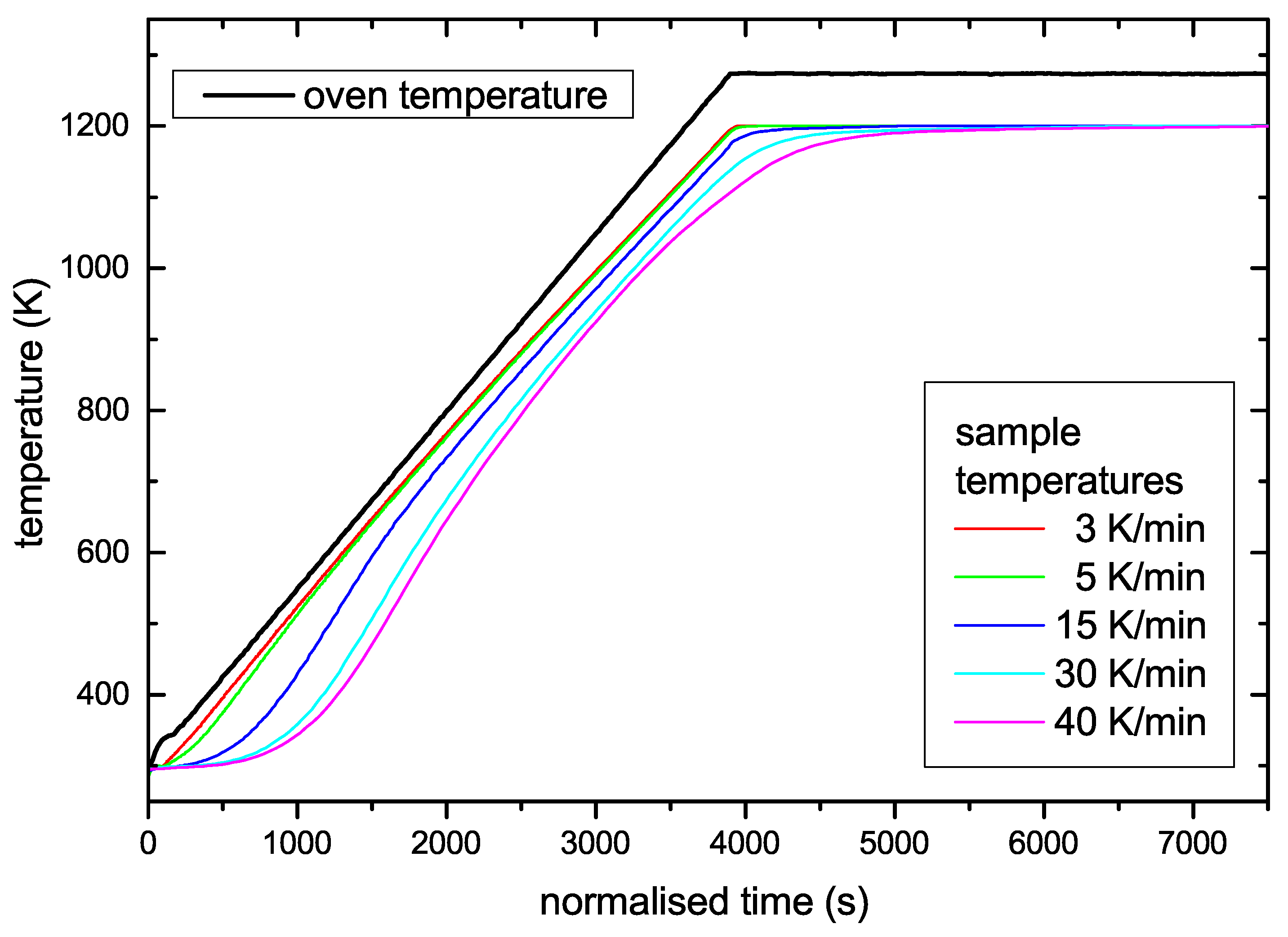
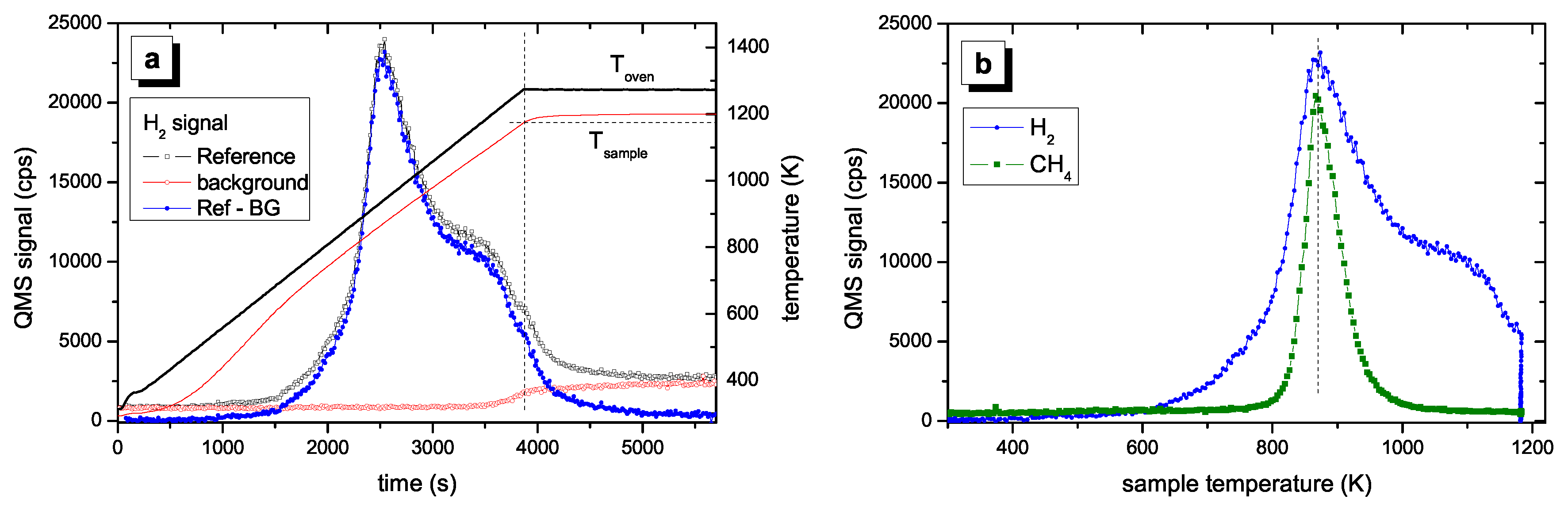
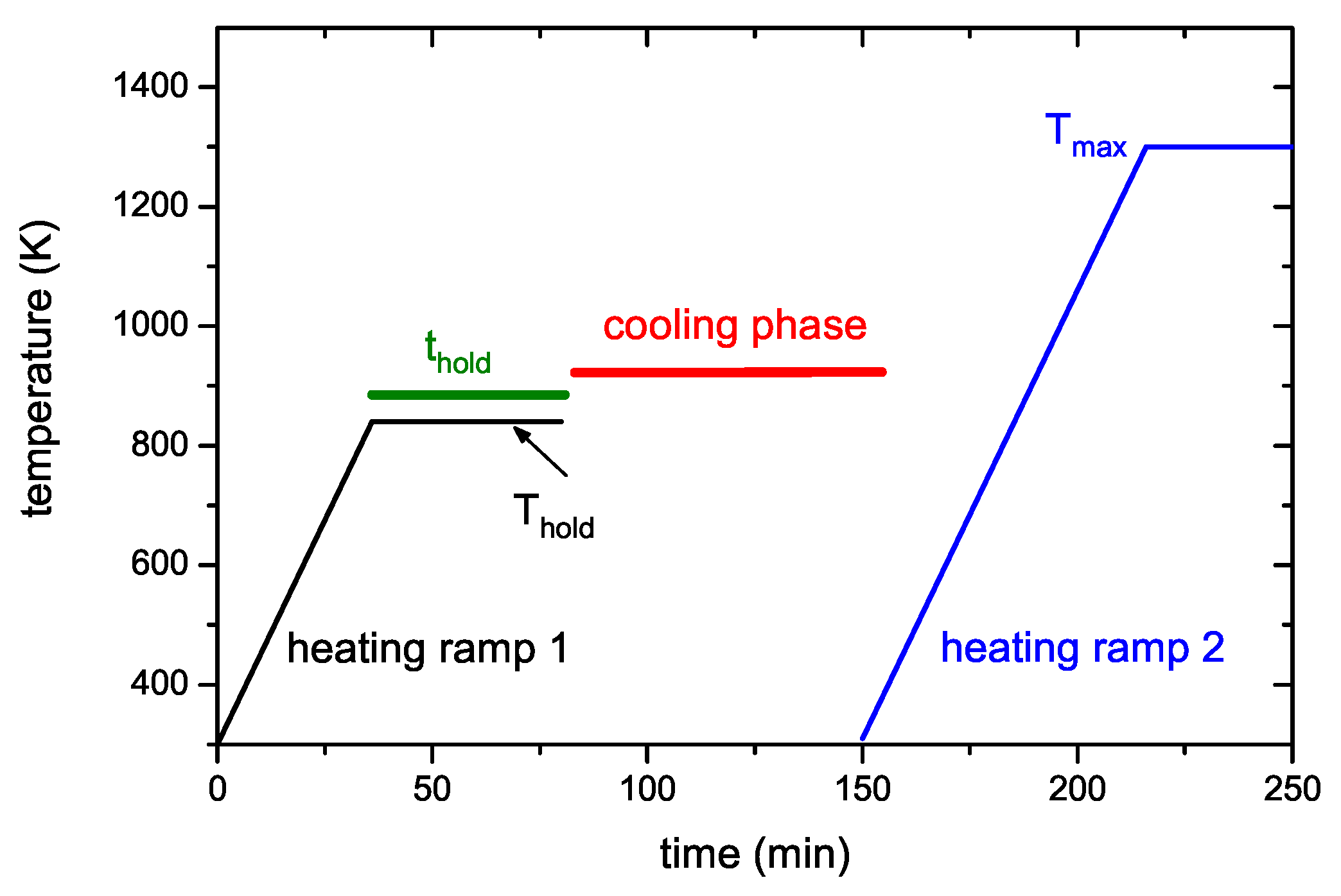
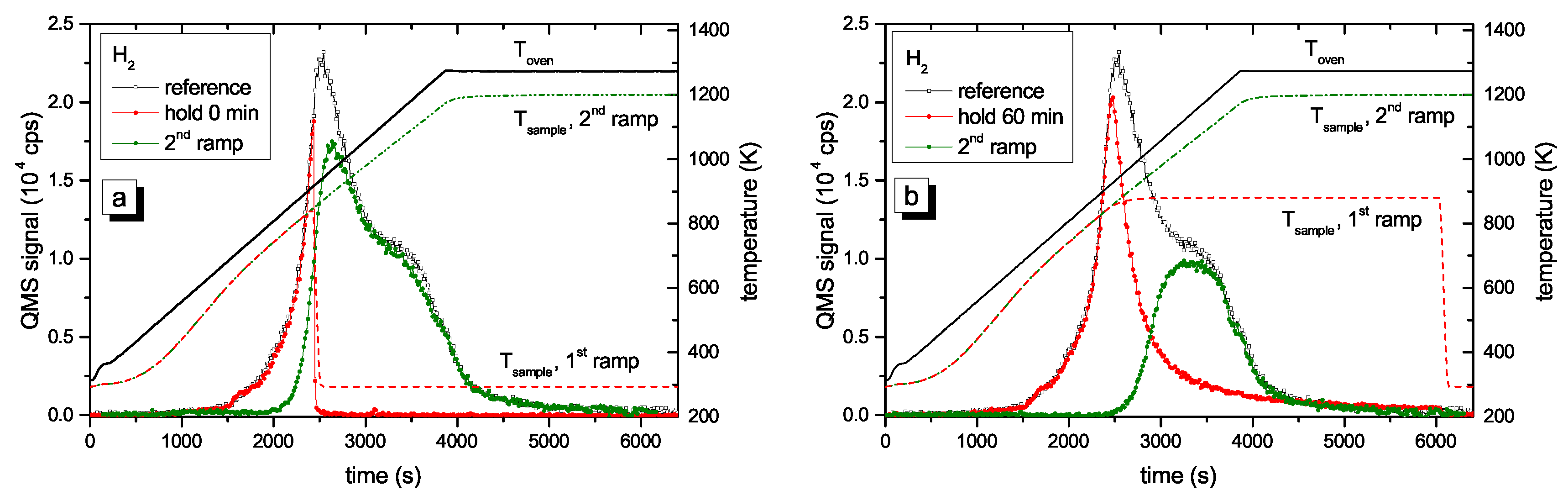
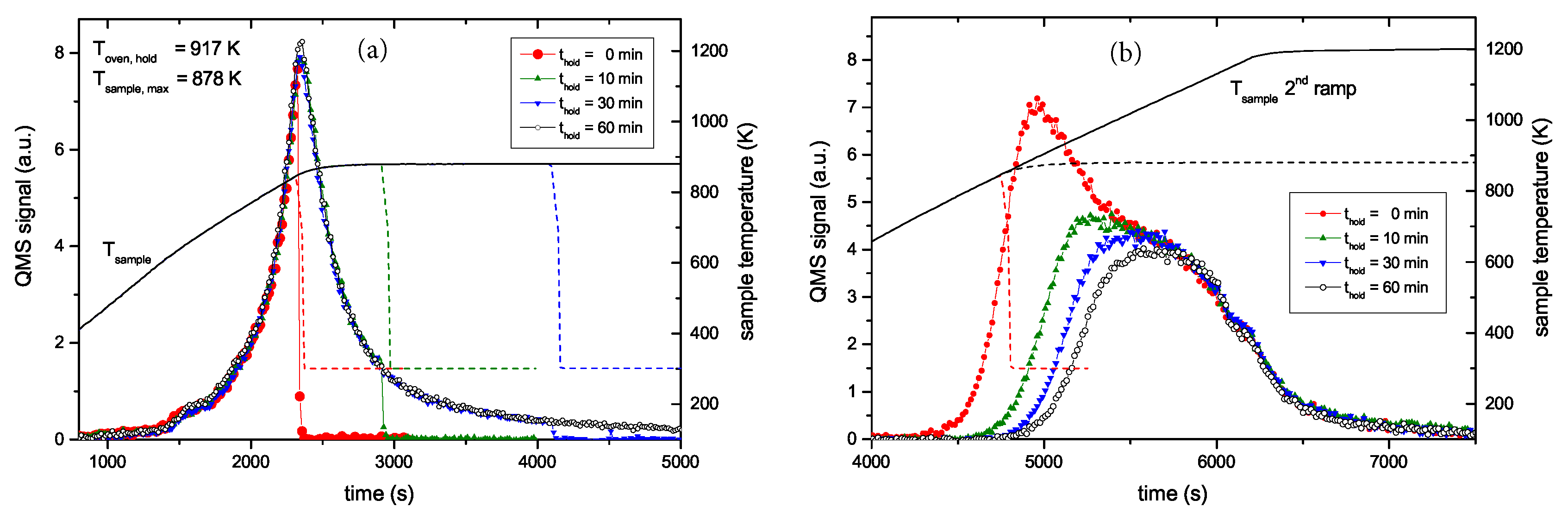
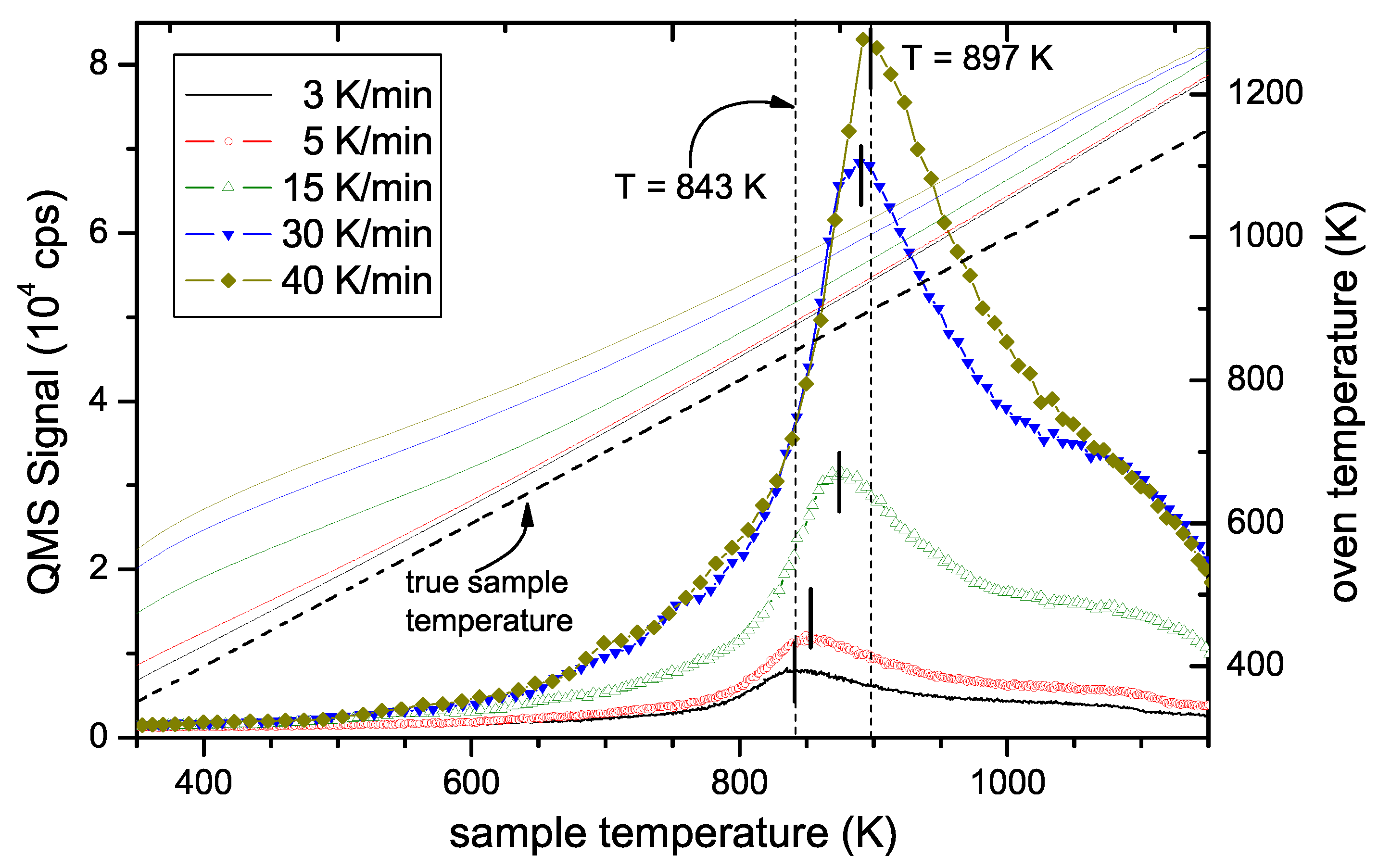
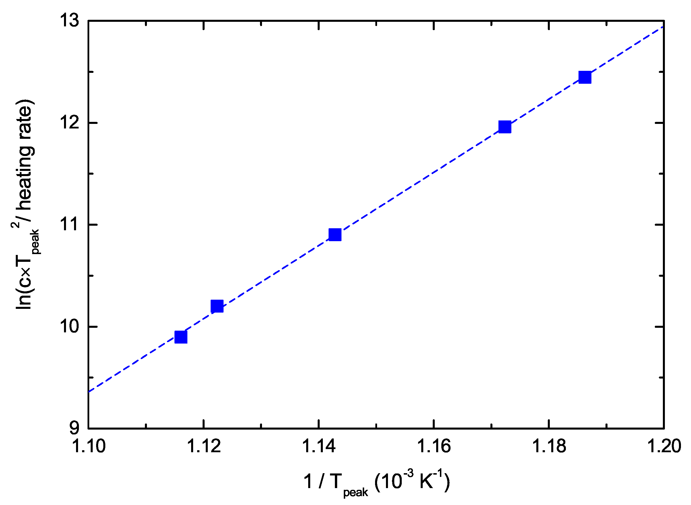
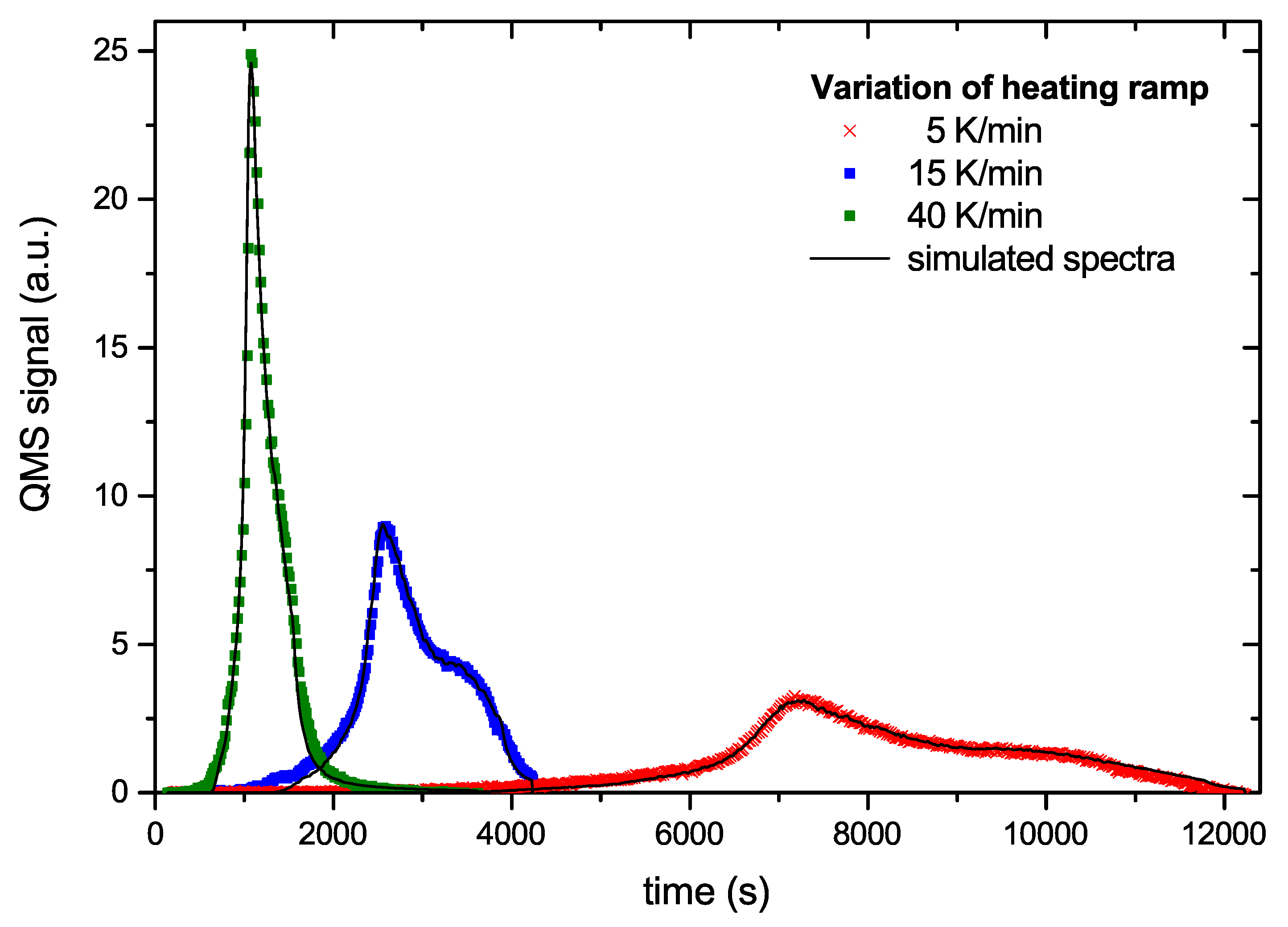
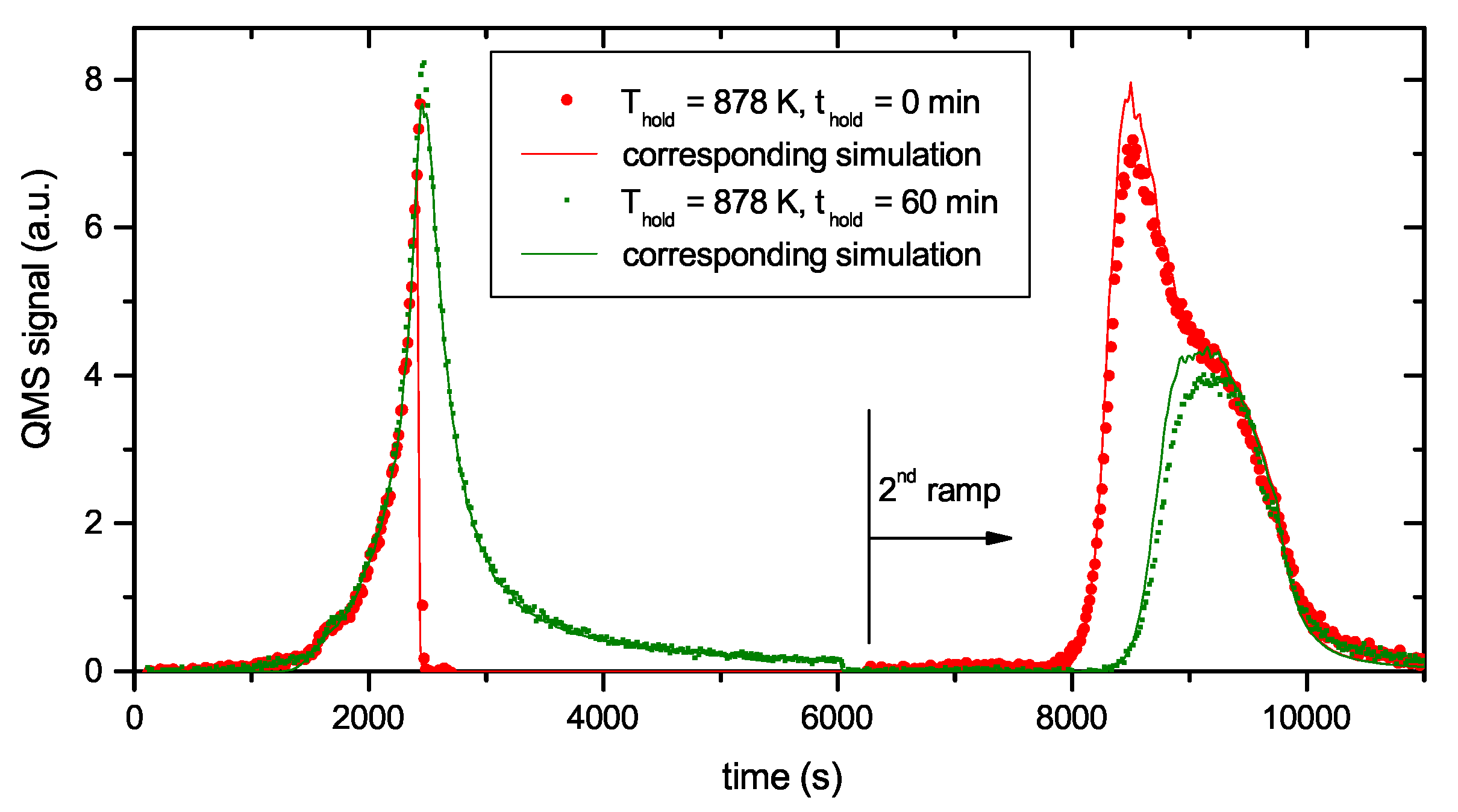
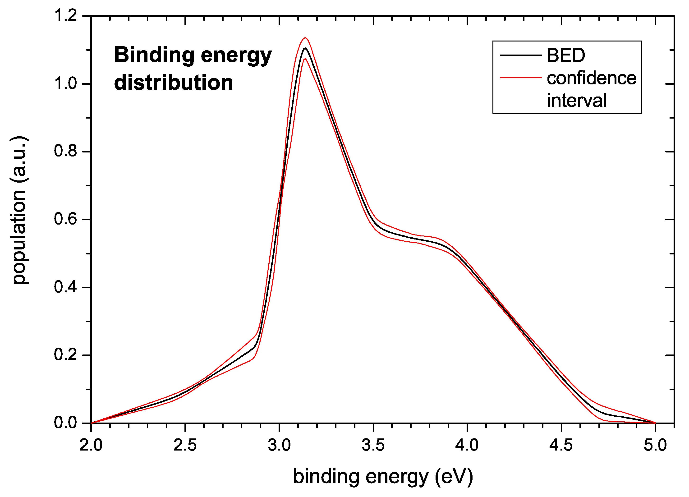
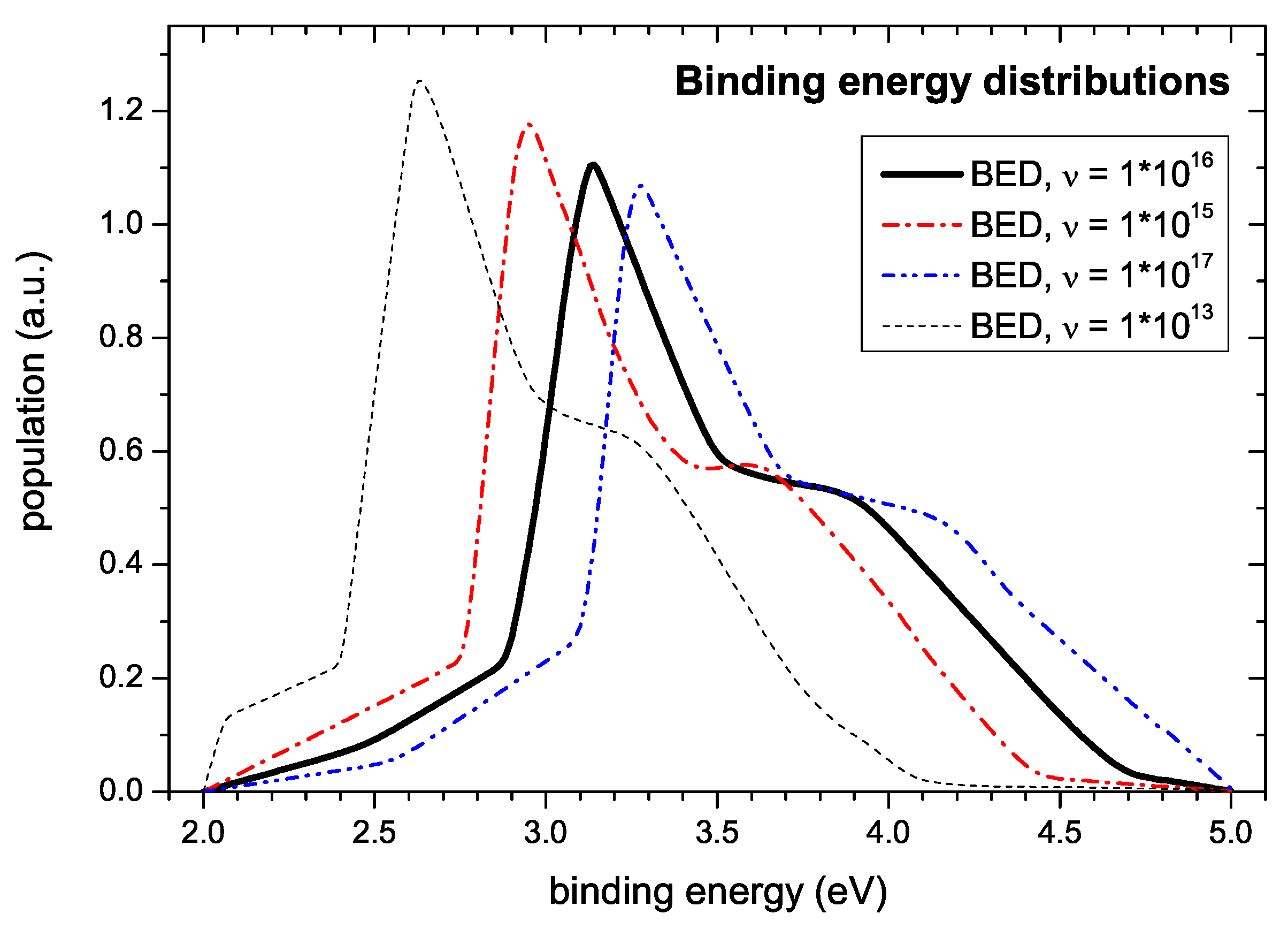
Table 1.
Different temperature ramps used in the experiment. Roven is the nominal temperature ramp of the external oven, Rsample is the corresponding measured temperature ramp of the sample at Tpeak. Tpeak is the measured sample temperature at which the maximum of the effusion peak occurs (see Figure 6).
| Roven (K/min) | Rsample (K/min) | Tpeak (K) |
|---|---|---|
| 3 | ||
| 5 | ||
| 15 | ||
| 30 | ||
| 40 |
Table 2.
Independent experiments used for the fit of the binding energy distribution. The table lists the type of experiment and the different experimental parameters that were used. Some data sets were measured twice (indicated by (2) behind the parmeter value). In that case both data sets were used for the fit.
| Type of Experiment | Experimental Parameters | No. of Spectra |
|---|---|---|
| normal TPD run | Roven = 5, 15 (2), 30, and 40 K/min | 5 |
| R&H experiment | Thold = 898 K, thold = 0 min | 1 |
| (Roven = 15 K/min) | Thold = 878 K, thold = 0 (2), 10, 30, and 60 min | 5 |
© 2020 by the authors. Licensee MDPI, Basel, Switzerland. This article is an open access article distributed under the terms and conditions of the Creative Commons Attribution (CC BY) license (http://creativecommons.org/licenses/by/4.0/).
Share and Cite
MDPI and ACS Style
Jacob, W.; Dürbeck, T.; Schwarz-Selinger, T.; von Toussaint, U. Bonding States of Hydrogen in Plasma-Deposited Hydrocarbon Films. C 2020, 6, 3. https://0-doi-org.brum.beds.ac.uk/10.3390/c6010003
AMA Style
Jacob W, Dürbeck T, Schwarz-Selinger T, von Toussaint U. Bonding States of Hydrogen in Plasma-Deposited Hydrocarbon Films. C. 2020; 6(1):3. https://0-doi-org.brum.beds.ac.uk/10.3390/c6010003
Chicago/Turabian StyleJacob, Wolfgang, Thomas Dürbeck, Thomas Schwarz-Selinger, and Udo von Toussaint. 2020. "Bonding States of Hydrogen in Plasma-Deposited Hydrocarbon Films" C 6, no. 1: 3. https://0-doi-org.brum.beds.ac.uk/10.3390/c6010003
Note that from the first issue of 2016, this journal uses article numbers instead of page numbers. See further details here.