Reducing the Computational Cost for Artificial Intelligence-Based Battery State-of-Health Estimation in Charging Events

Abstract

Powertrain electrification is bound to pave the way for the decarbonization process and pollutant emission reduction of the automotive sector, and strong attention should hence be devoted to the electrical energy storage system. Within such a framework, the lithium-ion battery plays a key role in the energy scenario, and the reduction of lifetime due to the cell degradation during its usage is bound to be a topical challenge. The aim of this work is to estimate the state of health (SOH) of lithium-ion battery cells with satisfactory accuracy and low computational cost. This would allow the battery management system (BMS) to guarantee optimal operation and extended cell lifetime. Artificial intelligence (AI) algorithms proved to be a promising data-driven modelling technique for the cell SOH prediction due to their great suitability and low computational demand. An accurate on-board SOH estimation is achieved through the identification of an optimal SOC window within the cell charging process. Several Bi-LSTM networks have been trained through a random-search algorithm exploiting constant current constant voltage (CCCV) test protocol data. Different analyses have been performed and evaluated as a trade-off between prediction performance (in terms of RMSE and customized accuracy) and computational burden (in terms of memory usage and elapsing time). Results reveal that the battery state of health can be predicted by a single-layer Bi-LSTM network with an error of 0.4% while just monitoring 40% of the entire charging process related to 60–100% SOC window, corresponding to the constant-voltage (CV) phase. Finally, results show that the amount of memory used for data logging and processing time has been cut by a factor of approximately 2.3.

1. Introduction

The necessity of reducing pollutant emissions caused by internal combustion engines of road vehicles and to increase the efficiency of the energy use in vehicles has led researchers to find new propulsion solutions. Electric motors have been used for road vehicle-propulsion systems for a long time (‘La Jamais Contente’ in 1899 was the first car in history that went beyond 100 km/h, and it was electric [1]; however, it was never used in production because of the difficulties in storing a large quantity of electric energy on vehicles). Recent technological advancements in Li-ion batteries partially fixed this problem and allowed electric motors to be employed for automotive traction. As a matter of fact, in contrast to many other electrical storage systems such as lead-acid batteries, Li-ion batteries have quite high energy and power density, a low level of self-discharge, a low need for maintenance, and good load characteristics, and they can be partially charged and discharged without being damaged [2,3,4]. If appropriately managed by a battery management system (BMS), Li-ion batteries can ensure an acceptable level of safety and valid lifespan, as essential requirements for automotive applications.

On the other hand, the Li-ion battery package is definitely the most critical and fragile component of the electric vehicle. In order to preserve battery health, it is extremely important to monitor and oversee its status while in operation. This is done by the BMS, which ensures that the battery pack works within its safe range and optimal conditions [5]. Cells must always operate within a specific range of temperature and voltage, and they cannot deliver excessively high currents. These conditions change from cell to cell depending on many factors, such as chemistry type. For instance, when batteries operate at excessively high temperatures, they may bloat with gas, causing leakage or explosion, or a thermal runaway may even occur [6,7]. As a result, the BMS must guarantee vehicle safety. Thermal management of cells is another key issue: at high temperatures, the battery degrades faster, leading to degradation of performance over time [8,9,10], while at low temperatures, the efficiency is lower due to the higher internal resistance of the cell [11]. Overvoltage and undervoltage conditions can also damage the battery chemistry [12,13]. In general, the more the batteries work far from their optimal temperature range which is commonly between −20 °C and 60 °C, the faster they degrade. According to the literature, although safe conditions are respected, batteries degrade at varying rates depending on the stress cycles. This is referred to as cyclic aging [14].

The BMS is critical to safeguard as much of the health and efficiency of the battery as possible, but it is also very important to know the battery health condition at any given time. When the battery degrades, its capacity reduces, producing a decrease in vehicle range, and its internal resistance increases. Specifically, the decrease in capacity impacts the amount of energy a battery can store, although the rise in internal resistance restricts the amount of power that can be generated [15]. For this reason, when battery capacity reaches 80% of its initial value or internal resistence reached 200% of the initial value, they are ordinarily not used any longer for automotive applications, and this is considered the conventional battery’s end of life (EOL). They can then be used for a variety of stationary applications, such as grid energy distribution, thus giving them a second life before recycling [16]. The health condition can be described by the state-of-health (SOH) parameter. In some applications where the power capacity is more significant than the energy amount, the internal resistance is generally regarded a SOH metric, and the SOH is therefore defined by the ratio between EOL and real internal resistance and EOL and fresh state internal resistance. In contrast, the SOH is defined as the ratio between the actual battery capacity and the capacity at the beginning of its life for applications wherein the available energy plays a significant role [17].

Therefore, depending on the application, capacity or internal resistance should be measured. Several techniques are proposed in the literature concerning the battery SOH estimation on board electric vehicles [18,19,20]. The battery aging state can be theoretically evaluated by knowing the history of the battery. A semi-empirical formula for the SOH identification has been exploited in [21,22], taking inspiration from the Arrenius equation for ideal gases’ behaviour and considering as the main aging agent the lithium-ion loss. This describes the dependency of the battery capacity loss on the number of cycles, temperature, charge, and discharge rate and depth of discharge. This formula may be useful both for estimating battery lifetime and for on-board applications. The equivalent circuit models (ECMs) are well-known model-based strategies that exhibit simplicity and good accuracy [23]. This method parameterizes the model variables in relation to the battery SOH by using experimental data [24]. For the battery aging status analysis, these models take into account the internal resistance increase. This can be accurately measured by using the electrochemical impedance spectroscopy (EIS) technology [25,26,27]. The EIS is a precise and reliable technique; however, nowadays it is rarely exploited for online applications. The high cost of the instruments required does not allow a large-scale use. Therefore, the internal resistence needs to be estimated on board with a different method. Many empirical data-driven models were developed to this end [28,29]. Among these, autoregressive models [30,31] and state observer models coupled with the extended Kalman filter [32,33] provided good results. A large number of different algorithms can be found, such as the particle swarm support vector machine algorithm (PSO-SVM) [34], a particle filter method [35], or even statistical methods [36]. Moreover, neural networks (NNs) seem to be a promising solution in giving accurate results [37,38,39,40,41]. In these studies, it is demonstrated that NNs continue to be research hotspots, exhibiting great potential in estimating SOH under complex aging conditions, particularly when the data are sufficiently abundant, owing to the advantages of approximation and learning speed. Briefly, ML-based SOH estimation approaches are research focuses and will have a significant impact on the future of transportation electrification. In particular, the feed-forward neural networks (FNNs), the convolutional neural networks (CNNs), and the recurrent long short-term memory (LSTM) are the best-performing NNs according to the literature. A comparison between them is given by Sungwoo Jo et al. (2021) [42] which shows the best performance belonging to LSTM compared with the others two types. However, LSTMs may require high computational cost and memory use due to the dimension of the memory cell and its complex structure.

The BMS handles the battery SOH identification task, as well as numerous other functions, including safety control, failure avoidance, and energy consumption optimization. Typically, automotive boards are supplied with ARM processors embedding a 32-bit architecture (multi-core), which can provide adequate processing power [43,44]. However, it is expected that more and more data and tasks will need to be stored and fulfilled as a consequence of technological advancements [43]. Performing some tasks by using external cloud devices could be a solution for this issue, yet it requires effective and reliable internet communication [45]. In [46], an LSTM for remaning useful life (RUL) estimation by using multichannel full charge profiles is presented, with considerable improvements over the baseline LSTM and a significant reduction in the amount of the parameters considered for the model. However, entire charge cycle data is employed, resulting in a large amount of memory and processing space. As a result, [47] develops an RNN-LSTM to estimate the RUL based on partial charge data in the voltage domain range, setting boundary limits. However, the complete SOC domain is not explored, and it is unclear how much memory and computational cost may be saved by varying the different SOC window lengths during charge for SOH estimation. Hence, the computational and memory use reduction for SOH estimation through a data-driven model is a current research gap.

To help fill the highlighted research gap, the main contribution of this study relates to the estimation of the battery SOH from partial charging data and varying the SOC window length through a bidirectional LSTM (Bi-LSTM) in order to reduce the on-board computational cost and memory use while maintaining a high degree of precision, consistent with other research studies in the literature that use the full charge data [48]. In particular, sensitivity analyses are performed to determine the minimum amount of data required in a battery charge process to ensure a good SOH estimation. Furthermore, the charge phase (in terms of SOC range) which is most reliable for the SOH estimation is assessed. This is done by training several Bi-LSTM NNs with data of charging made up of different lengths and considering different SOC windows. The Bi-LSTM neural network (NN) is a wide temporal prediction technique used for SOH estimation, and its predictive powers are derived from learning the forward and backward temporal correlation information in the input data [49,50]. As part of the learning process, many model parameters are automatically tuned based on the user-defined hyperparameters selected from a large pool of solutions. The best hyperparameter training combination has been determined separately for each experiment with a random-search algorithm. The final aim is to provide a light methodology from the computational and memory use points of view for the on-board estimation of the battery SOH, exploiting a data-logged time series that is as short as possible. Final results presented in the last part of this activity highlight that the method of partial charging data can be taken into account for the SOH on-board estimation to have a reduction of the computational demand at the control unit level with a saving of memory usage thanks to shorter data logging.

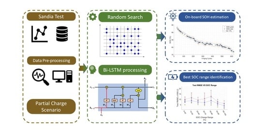
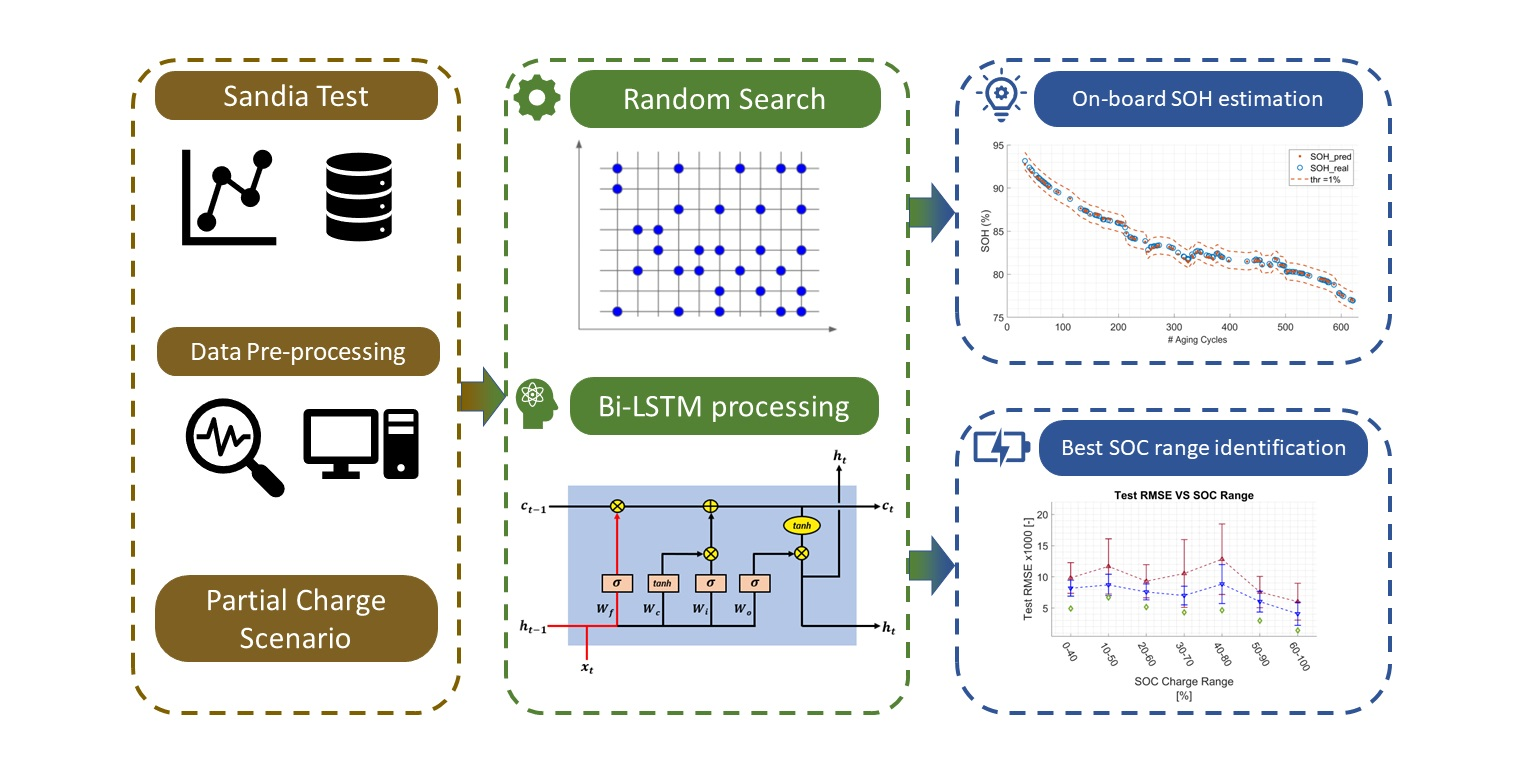
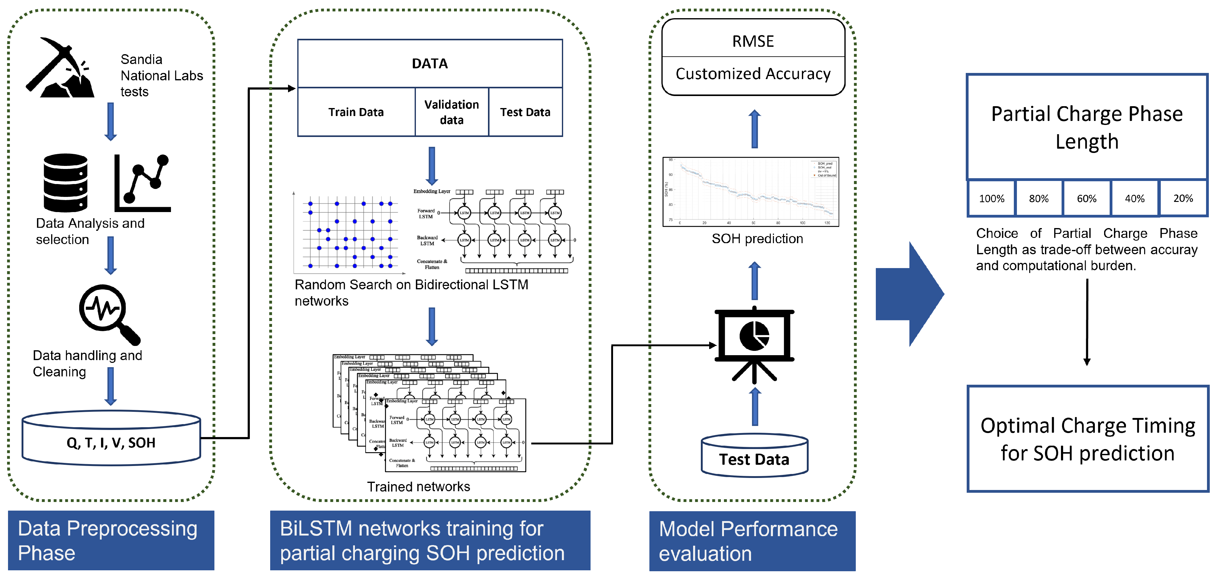
2. Materials and Methods

The current investigation involved estimating the remaining battery life while performing charge–discharge cycles. Several different cycle aging experimental tests have been performed in the literature [51] considering different cell chemistries. For our purpose, the selected aging dataset was that of Sandia National Laboratories [52]. This study has focused on the influence of cell operating conditions on long-term degradation of 18,650 nickel–manganese–cobalt (NMC) cells. Several bidirectional LSTM networks were created to investigate the accuracy in predicting the SOH prediction during partial charging phases with variable time lengths. The best SOC range for the SOH estimation during a single partial charging was finally evaluated. As a result, by knowing the optimal battery SOC window for SOH prediction, the battery’s health management system may be improved.

In this section, the proposed method composed by sequential steps is discussed and shown in Figure 1.

In the data processing phase, the cell signals acquired from cycle aging tests were analysed, handled, and cleaned. In the second step related to Bi-LSTM networks training phase, the data were split in training and validation datasets, and then exploited to perform the learning process of several Bi-LSTM architectures. The random search algorithm was used as a powerful hyperparameter tuning technique to find the most accurate network layout. Grid search and random search are often the most prevalent hyperparameter optimization approaches utilized for this purpose. From a computational cost standpoint, the latter enables the analysis of a larger number of neural networks to choose the best, hence lowering the time required to find the optimal hyperparameters [53]. During the learning process, the created dataset is randomly divided in training, validation, and test sets in order to train and validate the selected AI logics. Bi-LSTM NNs were used in this work due to their excellent capability and performance in time-series forecasting and learning the key paths in cell cycle aging events [54]. The Bi-LSTM is an extendend form of the baseline LSTM NN, and it is composed of two LSTM networks which process data in both forward and backward directions. An LSTM-based model contains a “gate” block that enables storing longer time sequences of data in the memory. Because Bi-LSTM models enable additional training by forward and backward data processing, Bi-LSTM-based modeling gives better performance and prediction with respect to regular LSTM-based models [55]. As with any AI model, the Bi-LSTM is defined by a set of hyperparameters that must be specified in order to tailor the model for the specific application. The random search optimization technique was used here to tune the hyperparameters [56]. In the final step, the performance of the identified best Bi-LSTM network was evaluated by considering a test dataset according to two different metrics, i.e., RMSE and a customized accuracy parameter. The described method was then exploited to find the best partial charging time length for the accurate and computationally lightweight estimation of the battery SOH. Finally, the most suitable SOC window for estimating the battery SOH during a vehicle charging event was assessed.

2.1. Data Preprocessing Phase

In the present work, the cell under examination was of 18,650 type with NMC chemistry on the cathode and graphite on the anode. The cycle aging tests have been performed by using a multi-channel battery testing system. Moreover, the cycle aging protocol is reported from Sandia National Laboratories [52]. A summary of test equipment and test operating conditions are, respectively, reported in

Table 1. Sandia National Laboratories equipment for cycle aging experiments [52].

Cell Type	Cathode	Anode	Capacity (Ah)	Test Equipment
18,650 NMC	NMC	graphite	3.00	High-precision Arbin

and

Table 2. Test operating conditions of cycle aging experiments. N° Cycles is the number of charge and discharge cycles that a cell can process before it reaches its end-of-life condition (20% of capacity loss).

Charge C Rate	Discharge Crate	SOC Range	Environmental Temperature (°C)	N° Cycles
0.50	2.00	0–100	25	661

.

The cell has been charged through a constant current constant voltage (CCCV) protocol, with 0.5 C current during CC phase and current taper to 0.05 A on CV. The NMC cell has been cycled from 2 to 4.2 V during all cycling tests for the whole SOC domain. A portion of the experimental test acquisition and the exploited CCCV protocol are reported in Figure 2.

The data acquisition system collected the following signals over time:

• Cycle index, number of charge–discharge cycle;
• Cell current [A];
• Cell voltage [V];
• Charge and discharge capacity [Ah];
• Charge and discharge energy [Wh];
• Cell temperature [°C];
• Environmental temperature [°C].

The SOH parameter was computed after the cell residual capacity has been determined at the end of each ith cycle by using Equation (1),

$$SO{H}_i=\frac{Q_{actual,i}}{Q_{rated}},$$

(1)

where $Q_{actual,i}$ is the capacity computed at the $i_{th}$ charge–discharge cycle and $Q_{rated}$ is the cell nominal capacity.

Before being used for training the AI algorithms, the acquired data were preprocessed by checking their robustness and quality. Examples include the identification and removal of anomalous traces, identified nans, and outliers of output signals. Additionally, the signals were cut so that the various case studies under consideration could take into account only the specific data of interest over time in order to accelerate the neural network training process. Finally, the acquired data were resempled from varying to constant frequency over time. Specifically, a sample time of 5 s is used to interpolate the considered data. Finally, the obtained dataset included a number of charging cycles from new cell conditions up to their EOL. Each cycle comprised of signals over time for cell temperature, voltage, current, charged capacity, and the corresponding SOH value.

2.2. AI Neural Networks Learning Process

The developed AI model, Bi-LSTM architectures, and the hyperparameters involved are shown in Figure 3.

The Bi-LSTM model had an input layer with the dimension of that input data, a batch normalization layer, a Bi-LSTM layer for learning long-term dependencies between cell parameters, and the SOH value to be predicted, a dropout layer to prevent overfitting [58], a fully connected layer for the SOH output forecasting, and the output layer, i.e., a regression layer that computed the loss function. As far as the training process is concerned, the training method reported in the box of Figure 3 was the algorithm used to perform optimization and is by far the most common way to optimize neural networks. An overview of all optimization technique can be seen in [59]. The learning phase lasts a certain number of epochs, which specifies how many times the whole dataset has been thoroughly processed.

This study focused on the estimation of SOH based on charge cycles, which are examples of time sequences. The problem is therefore based on sequence-to-one regression networks and the loss function is the half-mean-squared-error shown in the Equation (2),

$$Loss=\frac{1}{2}\sum _{i=1}^N\frac{{(\widehat{y_i}-y_i)}^2}{N},$$

(2)

where N is the number of responses, $y_i$ is the target output, and $\widehat{y_i}$ is the network’s prediction for response i. Finally, an early stopping tecnhique was applied when the performance of the validation phase started to degrade in order to avoid overfitting on training dataset [60].

2.3. Model Performance Evaluation

Each model was evaluated and selected by taking into account different performance metrics for the SOH prediction results. Together with test data, the performance of all trained Bi-LSTM architectures was analysed based on:

• the RMSE considering the test dataset,
• the coefficient of determination $R^2$, and
• the customized regression accuracy (CRA) coefficient, which compared the predicted SOH, $\widehat{SOH}$, with the corresponding measured value, $SOH$ through an identified threshold $thr$.

The specific performance evaluation of the neural networks and the selection of the best hyperparameter values are widely discussed and analysed in the Results and Discussion section.

2.4. Variable SOC Windows during Partial Charging Events

The time required to fully or partially charge the battery pack of an electric car is a crucial issue for most drivers. Depending on the charging power available from the grid, the battery pack charging process may take up to several hours. As a result, the current effort focused on determining the appropriate partial charging length as a trade-off in terms of accuracy and computational cost for on-board SOH estimation. Moreover, restraints in memory usage and data storage capacity is a widely known issue in modern on-board control units for passenger cars. Hence, reducing the data logged on the BMS could solve this problem. In particular, the shorter the length of partial charging data logged over time, the smaller the memory required and the computational cost for on-board data processing. Furthermore, the dataset sampling rate is a relevant aspect in memory use reduction. Due to the low dynamic range of the signal of interest, the sample rate for this activity has been set at 0.2 Hz.

The approach described in the previous section was developed in order to estimate the cell SOH by using only a portion of the data related to the overall battery charging process. In the first test scenario, before running the train–test split process regarding data, various lengths of partial charging segments over time were considered in the preprocessing step. In order to consider fixed portions of the 0–100% SOC window, the time lengths investigated were determined as a percentage. It should be noted that the more aged a cell is, the shorter the amount of data logged for a certain percentage of the SOC window due to capacity fading, as seen in Figure 4.

Therefore, different data series of partial charging were expressed as a percentage of the total SOC domain and the retained SOC intervals were:

• 80%
• 60%
• 40%
• 20%.

The partial charge segments were collected for each single cycle over time considering a random starting point. The cut point was randomly chosen among a certain area of points to guarantee that the segments were mathcing the whole length data. If $n_k$ is the length of the $k_{t}h$ cycle in terms of samples data over the entire SOC domain, L is the selected length as partial charging size related to the specific SOC window, the cut space S from which the segment starting point was randomly selected can be defined in Equation (3):

$$0\le S\le n_k-L.$$

(3)

Examples of retained partial charging segments, respectively related to SOC ranges of 80%, 60%, 40%, and 20% with respect to the entire SOC window, are highlighted in Figure 5.

In order to proceed with the learning process for the Bi-LSTM neural networks, the dataset of each partial charge segment was randomly subdivided into training, validation, and test data [61]. Here, an 80–20% split was retained between the training and validation dataset on one hand, and the test dataset on the other. The features were the cell operating parameters, such as voltage (V), current (A), charged capacity in time (Ah), and cell temperature (°C). The target was the SOH values to be predicted by the model.

2.5. Best Partial Charging Length and Optimal SOC Window Identification for SOH Estimation

In this section, Bi-LSTM networks were trained, and the optimal topologies for each charging length considered were identified. The purpose of the investigation was to determine the optimal SOC range for estimating the remaining life of a cell during its charging process. Before analyzing the best SOC window for the SOH estimation, it was necessary to determine the optimal partial charging length $L_{opt}$. Indeed, a trade-off between prediction accuracy (RMSE, CRA), computational cost and memory use was analysed for the on-board SOH estimation by control units of Li-ion battery packs.

A sensitivity analysis was conducted over the best 1, 5, and 10 Bi-LSTM networks considering RMSE and CRA for each charging length. The computational costs for each considered charging length were investigated, retaining the time required to run the numerical models for cell SOH estimation. Moreover, the memory storage capacity was analysed based on the memory used by the models and the data logged. Finally, the trade-off-based optimal input length was found and employed for the best SOC window analysis. A complete explanation of sensitivity and trade-off analysis will be described in the Results and Discussion section.

Once the optimal partial length $L_{opt}$ was obtained, a new dataset was generated by cutting data at different starting points among the full size data of cycles. Particularly, the cut points were defined at each 10% step in the SOC window until reaching the last point, which guaranteed the contiguous size of data, i.e., while respecting the 0% and 100% SOC limits. Hence, the SOC windows $SO{C}_{win}$ among the entire domain are shown in Equation (4) and expressed as a percentage of size data of a single charging cycle:

$$SO{C}_{L_{opt}}=[0;L_{opt}],[10;L_{opt}+10],\dots ,[100-L_{opt};100].$$

(4)

For instance, if the optimal length $L_{opt}$ was observed to be $40\%$, then the $SO{C}_{L_{opt}}$ is reported in Equation (5):

$$SO{C}_{40}=[0;40],[10;50],[20;60],[30;70],[40;80],[50;90],[60;100].$$

(5)

Considering the example of dataset shown in Figure 5 for $L_{opt}$ equal to 40%, the related charging data are illustrated in Figure 6.

In this analysis, once $L_{opt}$ was determined, the same split of data was preserved between training, validation, and test. This allowed for a careful analysis of the findings pertaining to the selection of the threshold value $thr$ utilized in the definition of the CRA, as stated in the Results and Discussion section.

As far as the learning process of the neural networks is concerned, the top 30 Bi-LSTM-trained networks from the previous section were used for a new learning process. However, the regression task, the feature definitions, and the target variable were identical. Finally, the optimal SOC range for capacity degradation estimation during charging events was determined.

3. Results and Discussion

In this work, an AI-based SOH estimator was developed considering partial charging of a Li-ion cell to reduce the computational cost and memory occupancy for BMS applications. As already detailed in the Materials and Methods section, cycle aging tests were exploited for model developing, and through an optimization technique Bi-LSTM network architectures were established for their high performance in forcasting task and managing time-dependent data.

Before delving further into the numerical findings, a broad view of the performance metrics retained in analyzing the outcomes must be provided. The performance of the trained models was assessed by taking into account the estimation capabilities over the test dataset. In general, the model outputs were studied by comparing them with real targets in terms of the absolute error shown in Equation (6). The main metrics considered in order to evaluate the quality of the model predictions were RMSE reported in Equation (7). The coefficient of determination $R^2$ is reported in Equation (8) along with the customized regression accuracy (CRA). The CRA parameter can be defined by considering the problem to be similar with a classification task whereby the result was evaluated as correct if the value of the absolute error was lower then a specific threshold, as shown in Equation (9). We have

$$E_i=x_i-\widehat{x_i}$$

(6)

$$RMSE=\sqrt{\frac{{\sum }_{i=1}^n{E_i}^2}{n}}$$

(7)

$$R^2=1-\frac{{\sum }_{i=1}^n{E}_i^2}{{\sum }_{i=1}^n{(x_i-\overline{x_i})}^2}$$

(8)

$$CRA=\frac{{\sum }_{i=1}^n{T}_i}{n}\times 100with:\left\{\begin{array}{c}{T}_i=1if\left|E_i\right|<threshold\hfill \\ T_i=0if\left|E_i\right|>threshold\hfill \end{array}\right.$$

(9)

$x_i$ was the target value, $\widehat{x_i}$ was the model output, $\overline{x_i}$ was the mean of the dataset label considering that each experimental test in the dataset had a number of samples equal to n, and $E_i$ is the residual between target and predicted values. All the results shown in this section are derived from the validation of the model on the testing data.

As seen in Figure 7, the $threshold$ value defines the accuracy of the model prediction.

In order to perform the sensitivity analysis, the best NN was determined for each charging length by minimizing the RMSE metric. Looking at Figure 7, the charging length equal to 40% is observed to have the most rapid growth and to be the only one reaching the 100% accuracy among the partial charging lengths. As far as the sensitivity analysis is concerned, a threshold of about 1% was chosen. Here, the threshold represents the tolerance of the estimated cell SOH compared with the related measurements. The 1% tolerance value appears to be consistent with the literature [62] because it has been demonstrated to limit the error in the cell SOH estimation within 2.2%. With the selected threshold value and for a partial length of 40%, the CRA reaches almost 80%. The results in Figure 7 are based on Analysis #1, where the training dataset for Bi-LSTM processing was created by randomly choosing several parts along the SOC domain in order to investigate which is the lower charging length and which still guarantees acceptable accuracy in cell SOH estimation. However, the overall accuracy of Analysis #1 is much lower than Analysis #3, where, in order to analyze which is the best SOC charging window for SOH estimation, each network was trained, respectively, with data from the same SOC window. Hence, in the latter analysis, the prediction results are far greater, and the threshold value may be drastically cut.

3.1. Analysis #1: Variable SOC Windows for Partial Charging

After the definition of the metrics involved in the analysis of the SOH estimation accuracy, the present section focuses on the study of the influence of each partial charging length over cell SOH forecasting. The trained model’s prediction results, in terms of CRA and RMSE are shown (after the training process phase was performed by the random-search technique) in Figure 8.

Specifically, the top one, five, and 10 trained Bi-LSTM networks are presented for each percentage of charging length analyzed based on the performance standard deviations. The overall trend of CRA is directly proportional to the length of the partial charging considered. Increasing the charging length from 20% to 40%, the test CRA of the five best networks increases by approximately 7%. From the test $RMSE$ point of view, even if the boundary cases 20% and 100% are, respectively, the worst and the best options, the trend of the five best networks changes. Being an AI model based on data, a large number of observations are required to find and recognize some specific patterns, especially when random approaches are exploited for generalization purposes. However, the objective of the study is to understand and investigate whether high accuracy can be attained for the cell SOH estimation with only partial charging events. For instance, looking at Figure 8, it can be seen that an accuracy level of roughly 77% can be attained by a network setup by using an input of 40% of the SOC window during a charge phase. The accuracy definition pertains to the CRA with a threshold parameter value of 1%. Given the customized nature of this metric and the randomness associated with the selection of hyperparameters and training data for the Analysis #1, a CRA value of 77% is not optimal (higher values are reached for the analysis #3). However, the 40% data length achieves very good RMSE and R2 scores compared to the literature. Moreover, excluding the 100% length case corresponding to the full SOC domain, the 40% data length case has the lowest RMSE error. This indicates that an optimal Bi-LSTM configuration is not found for each charging length case by the random process approach, although it is theoretically possible that this could occur after several additional iterations. Finally, the significant result of the analysis shows that the SOH of a cell can be carefully detected by just monitoring 40% of the whole 0–100% SOC charge process.

In Figure 9, the regression task results for the best Bi-LSTM network per each input charging length are represented.

As summary results,

Table 3. Analysis #1: Best neural network regression statistics.

Data Length [% of SOC]	100	80	60	40	20
m	2.67	5.82	9.92	8.81	3.68
q	0.97	0.93	0.88	0.89	0.96
Test RMSE × 1000	5.65	8.04	7.33	6.80	8.93
Test  $R^2$	0.99	0.97	0.96	0.96	0.96

and

Table 4. Analysis #1: Best neural network training and architecture parameters.

Data Length [% of SOC]	100	80	60	40	20
Hidden Layers	1	1	1	1	1
Hidden Neurons	59	30	29	47	52
State Activation Function	tanh	tanh	tanh	tanh	softsign
DropOut	0.2	0.3	0.2	0.1	0.1
Batch Size	128	32	64	32	64
Learning Rate	0.0090	0.0089	0.0060	0.0069	0.0044
Optimization Algorithm	sgdm	sgdm	adam	sgdm	adam
Training Epochs	190	84	108	264	186

resepectively report the validation performance of the developed models and the details of trained Bi-LSTM architectures for each SOC window length.

3.2. Analysis #2: Computational Cost and Memory Occupancy for Best SOC Charging Window Length Identification

In the on-board implementation of an SOH estimator, the computational power and memory occupancy are critical issues in current vehicle control units. In the present work, a profiling analysis was investigated as a performance metric together with $CRA$ and $RMSE$ in order to identify the best SOC window length for capacity fade monitoring. Hence, a profiling approach was developed to quantify the benefits of the proposed method in terms of computational costs and memory usage. In Figure 10, the computational performance required by the electronic control unit for the processing phase is shown.

The elapsed time in Figure 10 was computed by considering the average time for 10 runs among the best 30 neural networks for each charging dataset input length. The elapsed time seems to be almost linear. The computational time was processed through a laptop with Intel(R) Core (TM) i7-10510U CPU @ 1.80 GHz and 16 GB of RAM. The memory occupancy of stored data is plotted against input charging length and the figure clearly shows a linear behaviour. The longer the time series considered for the processing phase, the higher the space required by the memory. Finally, the memory used for the Bi-LSTM network size was computed as the required space to store the top 10 neural networks architectures for each data length. The main memory reduction factor is due to the dataset size reduction, which is clearly linear. On the other hand, the Bi-LSTM model sizes vary according to the same range (20 kB to 230 kB) for each input data length. As a consequence, the choice of the suitable SOC window length does not depend on the model dimension in this case.

3.3. Analysis #3: Best SOC Window Identification for Optimal SOH Estimation

Considering the results obtained by Analysis #1 and Analysis #2, it can be assumed that the configuration with the 40% length of input data is the best SOC window length $L_{opt}$ in terms of cell SOH estimation capability and computational lightweighting trade-off. Therefore, the present section is focused on this charging length value.

In this part, we investigated what specific part of the charge process contains more information about the battery SOH, allowing a better estimation of the battery’s remaining lifetime. The analysis results for $L_{opt}=40\%$ are shown in Figure 11.

As shown in Figure 11, higher performance in terms of $CRA$ and $RMSE$ are obtained due to an accurate reporting of the partial charging start points.

The presented analyses report that the last charging SOC window (with a range between 60% and 100%) guarantees the highest $CRA$ and the lowest $RMSE$ on the cell SOH estimation. Hence, this range is considered to be the optimal SOC window for the cell SOH estimation. Considering the input data representation in Figure 6, the optimal SOC charge range of 60% to 100% corresponds to the constant voltage (CV) phase of the charging process. The CCCV tests are widely employed for the cell SOH estimation and assessing the battery performance while aging [63]. Specifically, the partial CV charging phase is proven to be the most suitable for SOH estimation holding more information and robustness about capacity fade [64]. However, instead of considering a single CV trace, the present work compared and analysed different partial charging lengths over the entire charging process domain. In fact, concerning the best Bi-LSTM neural network, it is important to highlight that the other portions of the domain achieve remarkable results with a CRA accuracy that consistently approaches 90%. Moreover, it is interesting that the RMSE value for the 0–40% trace is only slightly higher, i.e., 0.0054, than the best value of 0.0012 for the 60–100% trace. However, it should be noted that evaluating the top 15 or 25 neural network configurations displays higher differences between the SOC windows. This confirms the prevalence of the typical aging pattern in a certain SOC range, i.e., 60–100%.

In Figure 12, the regression results for the best Bi-LSTM network for each SOC charge range considered were represented, and we can observe that the 60–100% range case has the smallest deviation in the regression line by bisector, and it has the predicted points densely packed on the bisector.

As summary results,

Table 5. Analysis #3: Best neural network regression statistics.

Charge Segment SOC [%]	0–40	10–50	20–60	30–70	40–80	50–90	60–100
m	0.96	0.90	0.96	1.02	0.98	0.98	0.99
q	3.29	7.99	3.82	−1.59	1.34	1.35	0.30
Test RMSE $\times 1000$	5.45	7.52	5.23	4.09	4.81	3.12	1.27
Test  $R^2$	0.98	0.95	0.98	0.99	0.98	0.99	0.99

and

Table 6. Analysis #3: Best neural network training and architecture parameters.

Charge Segment SOC [%]	0–40	10–50	20–60	30–70	40–80	50–90	60–100
Hidden Layers	1	1	1	1	1	1	1
Hidden Neurons	15	15	65	54	42	51	51
State Activation Function	tanh	tanh	softsign	softsign	tanh	softsign	softsign
DropOut	0.3	0.3	0.3	0.2	0.5	0.5	0.5
Batch Size	16	16	32	64	64	32	32
Learning Rate	0.0098	0.0098	0.0055	0.0099	0.0086	0.0083	0.0083
Optimization Algorithm	sgdm	sgdm	rmsprop	sgdm	sgdm	sgdm	sgdm
Training Epochs	92	30	43	155	103	91	62

show, resepectively, the validation performance of the developed models and the details of the trained Bi-LSTM architectures for each SOC charge range analysed.

3.4. Best SOC Window: Training and Validation Information

In this final section, training and validation performance details about the best Bi-LSTM network for the best SOC window of approimately 60–100% were discussed. As already explained, the performance in terms of $CRA$ and $RMSE$ of this trained network with the homogeneous dataset are much more analytically compared with Figure 8 and Figure 9 from Analysis #1. The statistical metrics and Bi-LSTM architecture details are those shown in Table 5 and Table 6. In Figure 13, the training history along the epochs are reported, comparing the loss function between the training dataset and validation dataset.

The learning process shows a trend that seems to be in line with good fit results, thus excluding overfitting and underfitting of a training phase. Finally, Figure 14 plots the SOH predicted points as those composing the test set among all aging cycles.

The results shown in the figure ensure promising performance in SOH estimation capability reaching 100% CRA and a low residual error for each cycle prediction, i.e., that the uncertainty of prediction is within 1%. However, because of the strong forecasting performance, it is feasible to achieve the same accuracy value of 100% in an area of uncertainty (threshold) decreased to 0.4% by analyzing the punctual error. For the sake of clarity, the CRA defines the percentage by which a model estimation may fall within a given uncertainty range of the target. The amplitude of the range is described by the threshold parameter value.

4. Conclusions

This study proposed a computationally lightweight methodology for the cell SOH estimation on board electric vehicles during partial charging processes. Several Bi-LSTM neural networks were trained, exploiting different datasets made of battery-charging data time series with varying lengths and random selection of the start point within the battery SOC domain. The proposed methodology identified the best SOC window length as a trade-off between the prediction accuracy and the computational cost for on-board SOH estimation. Moreover, the optimal SOC charge range which allows higher performance for the cell SOH estimation is identified. The proposed neural network considers time series made of the cell current, voltage, temperature, and the capacity charged while the output is the single regression value of the SOH. The case study retains an 18,650 cell with 3 Ah capacity and nickel–manganese–cobalt chemistry whereas the dataset is part of a collection of cycle aging tests performed by the Sandia Nation Laboratories. The results are consistent and show that the battery SOH can be predicted with the highest error of ±0.4%, monitoring just the last 40% of the SOC window (CV phase) of the total CCCV charge process by reducing the memory occupancy in the BMS for charge data logging and the computational time by a factor of about 2.3. Just a single cell operating condition has been considered in this study, consisting of charging and discharging at constant current and environmental temperature. In future work, the methodology could be extended to a wider range of working conditions, including additional temperatures, charging and discharging operations. Furthermore, the length of the charge segment to be monitored has been identified through a process that does not allow us to find the globally optimal solution. Therefore, additional improvements could be obtained by developing appropriate fine-tuning methodologies. An additional future development concerns the study of optimization of Bi-LSTM neural network architectures constrained to having smaller dimensions.

References

1. Van den Bossche, A. Light and Ultralight electric vehicles. In 4ième Conférence Internationale sur le Génie Electrique (CIGE 2010) (No. 2, pp. 3–9); Université de Bechar Algérie: Béchar, Algeria, 2010. [Google Scholar]
2. Blomgren, G.E. The Development and Future of Lithium Ion Batteries. J. Electrochem. Soc. 2016, 164, A5019. [Google Scholar] [CrossRef] [Green Version]
3. Keshan, H.; Thornburg, J.; Ustun, T.S. Comparison of lead-acid and lithium ion batteries for stationary storage in off-grid energy systems. In Proceedings of the 2016 4th IET Clean Energy and Technology Conference, Kuala Lumpur, Malaysia, 14–15 November 2019. [Google Scholar]
4. Vutetakis, D.; Timmons, J. A Comparison of Lithium-Ion and Lead-Acid Aircraft Batteries. SAE Tech. Paper 2008, 1, 2875. [Google Scholar]
5. See, K.W.; Wang, G.; Zhang, Y.; Wang, Y.; Meng, L.; Gu, X.; Zhang, N.; Lim, K.C.; Zhao, L.; Xie, B. Critical review and functional safety of a battery management system for large-scale lithium-ion battery pack technologies. Int. J. Coal. Sci. Technol. 2022, 9, 36. [Google Scholar] [CrossRef]
6. Feng, X.; Ouyang, M.; Liu, X.; Lu, L.; Xia, Y.; He, X. Thermal runaway mechanism of lithium ion battery for electric vehicles: A review. Energy Storage Mater. 2017, 10, 246–267. [Google Scholar] [CrossRef]
7. Tran, M.K.; Mevawalla, A.; Aziz, A.; Panchal, S.; Xie, Y.; Fowler, M. A Review of Lithium-Ion Battery Thermal Runaway Modeling and Diagnosis Approaches. Processes 2022, 10, 1192. [Google Scholar] [CrossRef]
8. Leng, F.; Tan, C.; Pecht, M. Effect of Temperature on the Aging rate of Li Ion Battery Operating above Room Temperature. Sci. Rep. 2015, 5, 12967. [Google Scholar] [CrossRef] [Green Version]
9. Ma, S.; Jiang, M.; Tao, P.; Song, C.; Wu, J.; Wang, J.; Deng, T.; Shang, W. Temperature effect and thermal impact in lithium-ion batteries: A review. Prog. Nat. Sci. Mater. Int. 2018, 28, 6. [Google Scholar] [CrossRef]
10. Jaydeep, B. Effect of Temperature on Battery Life and Performance in Electric Vehicle. Int. J. Sci. Res. 2012, 2, 1–3. [Google Scholar]
11. Ouyang, D.; He, Y.; Weng, J.; Liu, J.; Chen, M.; Wang, J. Influence of low temperature conditions on lithium-ion batteries and the application of an insulation material. RSC Adv. 2019, 9, 9053–9066. [Google Scholar] [CrossRef] [Green Version]
12. Hossein, M.; Jason, H. Effects of overdischarge on performance and thermal stability of a Li-ion cell. J. Power Sources 2006, 160, 1395–1402. [Google Scholar]
13. Xu, B.; Oudalov, A.; Ulbig, A.; Andersson, G.; Kirschen, D.s. Modeling of Lithium-Ion Battery Degradation for Cell Life Assessment. IEEE Trans. Smart Grid 2016, 99, 1. [Google Scholar] [CrossRef]
14. Raj, T.; Wang, A.A.; Monroe, C.W.; Howey, D.A. Investigation of Path-Dependent Degradation in Lithium-Ion Batteries. Eur. Chem. Soc. Publ. 2020, 3, 12. [Google Scholar] [CrossRef]
15. Barcellona, S.; Colnago, S.; Dotelli, G.; Latorrata, S.; Piegari, L. Aging effect on the variation of Li-ion battery resistance as function of temperature and state of charge. J. Energy Storage 2022, 50, 104658. [Google Scholar] [CrossRef]
16. Shahjalal, M.; Roy, P.K.; Shams, T.; Fly, A.; Chowdhury, J.I.; Ahmed, R.; Liu, K. A review on second-life of Li-ion batteries: Prospects, challenges, and issues. Energy 2022, 241, 122881. [Google Scholar] [CrossRef]
17. Shu, X.; Shen, S.; Shen, J.; Zhang, Y.; Li, G.; Chen, Z.; Liu, Y. State of health prediction of lithium-ion batteries based on machine learning: Advances and perspectives. iScience 2021, 24, 11. [Google Scholar] [CrossRef] [PubMed]
18. Lin, C.; Tang, A.; Wang, W. A Review of SOH Estimation Methods in Lithium-ion Batteries for Electric Vehicle Applications. Energy Procedia 2015, 75, 1920–1925. [Google Scholar] [CrossRef] [Green Version]
19. Berecibar, M.; Gandiaga, I.; Villarreal, I.; Omar, N.; Van Mierlo, J.; Van den Bossche, P. Critical review of state of health estimation methods of Li-ion batteries for real applications. Renew. Sustain. Energy Rev. 2016, 56, 572–587. [Google Scholar] [CrossRef]
20. Noura, N.; Boulon, L.; Jemeï, S. A Review of Battery State of Health Estimation Methods: Hybrid Electric Vehicle Challenges. World Electr. Veh. J. 2020, 11, 66. [Google Scholar] [CrossRef]
21. Han, H.; Xu, H.; Yuan, Z.; Shen, Y. A new SOH prediction model for lithium-ion battery for electric vehicles. In Proceedings of the 2014 17th International Conference on Electrical Machines and Systems (ICEMS), Hangzhou, China, 22–25 October 2014. [Google Scholar]
22. Anselma, P.G.; Kollmeyer, P.; Lempert, J.; Zhao, Z.; Belingardi, G.; Emadi, A. Battery state-of-health sensitive energy management of hybrid electric vehicles: Lifetime prediction and ageing experimental validation. Appl. Energy 2021, 285, 116440. [Google Scholar] [CrossRef]
23. Falai, A.; Giuliacci, T.A.; Misul, D.; Paolieri, G.; Anselma, P.G. Modeling and On-Road Testing of an Electric Two-Wheeler towards Range Prediction and BMS Integration. Energies 2022, 15, 2431. [Google Scholar] [CrossRef]
24. Amir, S.; Gulzar, M.; Tarar, M.O.; Naqvi, I.H.; Zaffar, N.A.; Pecht, M.G. Dynamic Equivalent Circuit Model to Estimate State-of-Health of Lithium-Ion Batteries. IEEE Access 2022, 10, 18279–18288. [Google Scholar] [CrossRef]
25. Galeotti, M.; Cinà, L.; Giammanco, C.; Cordiner, S.; Di Carlo, A. Performance analysis and SOH (state of health) evaluation of lithium polymer batteries through electrochemical impedance spectroscopy. Energy 2015, 89, 678–686. [Google Scholar] [CrossRef]
26. Kieran, M.; Hemtej, G.; Kevin, M.R.; Tadhg, K. Review—Use of impedance spectroscopy for the estimation of Li-ion battery state of charge, state of health and internal temperature. J. Electrochem. Soc. 2021, 168, 080517. [Google Scholar]
27. Sihvo, J.; Roinila, T.; Stroe, D.I. SOH analysis of Li-ion battery based on ECM parameters and broadband impedance measurements. In Proceedings of the IECON 2020 the 46th Annual Conference of the IEEE Industrial Electronics Society, Singapore, 18–21 October 2020. [Google Scholar]
28. Preetpal, S.; Che, C.; Cher, T.; Shyh-Chin, H. Semi-Empirical Capacity Fading Model for SoH Estimation of Li-Ion Batteries. Appl. Sci. 2019, 9, 3012. [Google Scholar]
29. Huanyang, H.; Jinhao, M.; Yuhong, W.; Lei, C.; Jichang, P.; Ji, W.; Qian, X.; Tianqi, L.; Remus, T. An Enhanced Data-Driven Model for Lithium-Ion Battery State-of-Health Estimation with Optimized Features and Prior Knowledge. Automot. Innov. 2022, 5, 134–145. [Google Scholar] [CrossRef]
30. Huang, J.; Wang, S.; Xu, W.; Shi, W.; Fernandez, C. A Novel Autoregressive Rainflow—Integrated Moving Average Modeling Method for the Accurate State of Health Prediction of Lithium-Ion Batteries. Processes 2021, 9, 795. [Google Scholar] [CrossRef]
31. Gao, K.; Xu, J.; Li, Z.; Cai, Z.; Jiang, D.; Zeng, A. A Novel Remaining Useful Life Prediction Method for Capacity Diving Lithium-Ion Batteries. ACS Omega 2022, 7, 26701–26714. [Google Scholar] [CrossRef]
32. Pang, B.; Chen, L.; Dong, Z. Data-Driven Degradation Modeling and SOH Prediction of Li-Ion Batteries. Energies 2022, 15, 5580. [Google Scholar] [CrossRef]
33. Azis, N.A.; Joelianto, E.; Widyotriatmo, A. State of Charge (SoC) and State of Health (SoH) Estimation of Lithium-Ion Battery Using Dual Extended Kalman Filter Based on Polynomial Battery Model. In Proceedings of the 2019 6th International Conference on Instrumentation, Control, and Automation (ICA), Bandung, Indonesia, 31 July–2 August 2019. [Google Scholar]
34. Li, R.; Li, W.; Zhang, H.; Zhou, Y.; Tian, W. On-Line Estimation Method of Lithium-Ion Battery Health Status Based on PSO-SVM. Front. Energy Res. 2021, 9, 401. [Google Scholar] [CrossRef]
35. Bian, Z.; Ma, Y. An Improved Particle Filter Method to Estimate State of Health of Lithium-Ion Battery. IFAC-PapersOnLine 2021, 54, 344–349. [Google Scholar] [CrossRef]
36. Chinedu, O.; Nagarajan, R. Statistical Characterization of the State-of-Health of Lithium-Ion Batteries with Weibull Distribution Function—A Consideration of Random Effect Model in Charge Capacity Decay Estimation. Batteries 2012, 3, 32. [Google Scholar]
37. Sui, X.; He, S.; Vilsen, S.B.; Meng, J.; Teodorescu, R.; Stroe, D. A review of non-probabilistic machine learning-based state of health estimation techniques for Lithium-ion battery. Appl. Energy 2021, 300, 117346. [Google Scholar] [CrossRef]
38. Bao, Z.; Jiang, J.; Zhu, C.; Gao, M. A New Hybrid Neural Network Method for State-of-Health Estimation of Lithium-Ion Battery. Energies 2022, 15, 4399. [Google Scholar] [CrossRef]
39. Zhou, J.; He, Z.; Gao, M.; Liu, Y. Battery state of health estimation using the generalized regression neural network. In Proceedings of the 2015 8th International Congress on Image and Signal Processing (CISP), Shenyang, China, 14–16 October 2015. [Google Scholar]
40. Jiantao, Q.; Feng, L.; Yuxiang, M.; Jiaming, F. A Neural-Network-based Method for RUL Prediction and SOH Monitoring of Lithium-Ion Battery. IEEE Access 2019, 1, 1. [Google Scholar]
41. Fan, Y.; Wu, H.; Chen, W.; Jiang, Z.; Huang, X.; Chen, S.-Z. A Data Augmentation Method to Optimize Neural Networks for Predicting SOH of Lithium Batteries. In Proceedings of the International Conference on Robotics Automation and Intelligent Control (ICRAIC 2021), Wuhan, China, 26–28 November 2021. [Google Scholar]
42. Jo, S.; Jung, S.; Roh, T. Battery State-of-Health Estimation Using Machine Learning and Preprocessing with Relative State-of-Charge. Energies 2021, 14, 7206. [Google Scholar] [CrossRef]
43. Morello, R.; Di Rienzo, R.; Roncella, R.; Saletti, R.; Schwarz, R.; Lorentz, V.R.; Hoedemaekers, E.R.G.; Rosca, B.; Baronti, F. Advances in Li-Ion Battery Management for Electric Vehicles. In Proceedings of the IECON 2018—44th Annual Conference of the IEEE Industrial Electronics Society, Washington, DC, USA, 21–23 October 2018. [Google Scholar]
44. Gabbar, H.A.; Othman, A.M.; Abdussami, M.R. Review of Battery Management Systems (BMS) Development and Industrial Standards. Technologies 2021, 9, 28. [Google Scholar] [CrossRef]
45. Yang, S.; Zhang, Z.; Cao, R.; Wang, M.; Cheng, H.; Zhang, L.; Jiang, Y.; Li, Y.; Chen, B.; Ling, H.; et al. Implementation for a cloud battery management system based on the CHAIN framework. Energy AI 2021, 5, 100088. [Google Scholar] [CrossRef]
46. Park, K.; Choi, Y.; Choi, W.J.; Ryu, H.-Y.; Kim, H. LSTM-Based Battery Remaining Useful Life Prediction With Multi-Channel Charging Profiles. IEEE Access 2020, 8, 20786–20798. [Google Scholar] [CrossRef]
47. Cinomona, B.; Chung, C.; Tsai, M.-C. Long Short-Term Memory Approach to Estimate Battery Remaining Useful Life Using Partial Data. IEEE Access 2020, 8, 165419–165431. [Google Scholar] [CrossRef]
48. Gong, D.; Gao, Y.; Kou, Y.; Wang, Y. State of health estimation for lithium-ion battery based on energy features. Energy 2022, 257, 124812. [Google Scholar] [CrossRef]
49. Sun, S.; Sun, J.; Wang, Z.; Zhou, Z.; Cai, W. Prediction of Battery SOH by CNN-Bi-LSTM Network Fused with Attention Mechanism. Energies 2022, 15, 4428. [Google Scholar] [CrossRef]
50. Pham, T.; Truong, L.; Nguyen, M.; Garg, A.; Gao, L.; Quan, T. Sequence-in-Sequence Learning for SOH Estimation of Lithium-Ion Battery. In Proceedings of the 11th International Conference on Electronics, Communications and Networks (CECNet), Xiamen, China, 18–21 November 2021. [Google Scholar]
51. Dos Reis, G.; Strange, C.; Yadavc, M.; Li, S. Lithium-ion battery data and where to find it. Energy&AI 2021, 5, 100081. [Google Scholar]
52. Sandia National Lab. Data for Degradation of Commercial Lithium-Ion Cells as a Function of Chemistry and Cycling Conditions. 2020. Available online: https://www.batteryarchive.org/snl_study.html (accessed on 10 June 2022).
53. Medium. A Comparison of Grid Search and Randomized Search Using Scikit Learn. 2019. Available online: https://medium.com/@peterworcester_29377/a-comparison-of-grid-search-and-randomized-search-using-scikit-learn-29823179bc85 (accessed on 8 July 2022).
54. Khan, N.; Ullah, F.U.M.; Ullah, A.; Lee, M.Y.; Baik, S.W. Batteries State of Health Estimation via Efficient Neural Networks With Multiple Channel Charging Profiles. IEEE Access 2020, 9, 7797–7813. [Google Scholar] [CrossRef]
55. Siami-Namini, S.S.; Tavakoli, N.T.; Siami Namin, A.S.N. The Performance of LSTM and Bi-LSTM in Forecasting Time Series. In Proceedings of the IEEE International Conference on Big Data, Los Angeles, CA, USA, 9–12 December 2019. [Google Scholar]
56. Machine Learning Mastery. Hyperparameter Optimization with Random Search and Grid Search. 2020. Available online: https://machinelearningmastery.com/hyperparameter-optimization-with-random-search-and-grid-search/ (accessed on 15 August 2022).
57. Mathworks. Deep Learning with Time Series and Sequence Data. Available online: https://www.mathworks.com/help/deeplearning/deep-learning-with-time-series-sequences-and-text.html (accessed on 15 August 2022).
58. Machine Learning Mastery. A Gentle Introduction to Dropout for Regularizing Deep Neural Networks. 2018. Available online: https://machinelearningmastery.com/dropout-for-regularizing-deep-neural-networks/ (accessed on 15 August 2022).
59. Sebastian Ruder. An Overview of Gradient Descent Optimization Algorithms. 2016. Available online: https://ruder.io/optimizing-gradient-descent/ (accessed on 15 August 2022).
60. Machine Learning Mastery. A Gentle Introduction to Early Stopping to Avoid Overtraining Neural Networks. 2018. Available online: https://machinelearningmastery.com/early-stopping-to-avoid-overtraining-neural-network-models/ (accessed on 20 August 2022).
61. Machine Learning Mastery. Train-Test Split for Evaluating Machine Learning Algorithms. 2020. Available online: https://machinelearningmastery.com/train-test-split-for-evaluating-machine-learning-algorithms/ (accessed on 20 August 2022).
62. Shi, M.; Xu, J.; Lin, C.; Mei, X. A fast state-of-health estimation method using single linear feature for lithium-ion batteries. Energy 2022, 256, 124652. [Google Scholar] [CrossRef]
63. Bin, X.; Bing, X.; Luoshi, L. State of Health Estimation for Lithium-Ion Batteries Based on the Constant Current–Constant Voltage Charging Curve. Electronics 2020, 9, 1279. [Google Scholar]
64. Ruan, H.; He, H.; Wei, Z.; Quan, Z.; Li, Y. State of Health Estimation of Lithium-ion Battery Based on Constant-Voltage Charging Reconstruction. IEEE J. Emerg. Sel. Top. Power Electron. 2021. [Google Scholar] [CrossRef]
Figure 1. The proposed methodology for battery SOH prediction during partial charging processes.
Batteries 08 00209 g001
Figure 2. Example of constant current constant voltage charge profiles measured by Sandia National Laboratories during the performed experimental cell aging campaign. The cell operating parameters measured during the tests are (a) cell voltge (V), (b) current (A), (c) charged and discharged capacity (Ah), and (d) cell and environmental temperature (°C).
Batteries 08 00209 g002
Figure 3. AI model graph based on Bi-LSTM network and hyperparameters investigated by the random-search optimization technique. The input layer normalizes data with the z-score method. A batch normalization layer normalizes a batch of data across all observations. The Bi-LSTM layer is defined by the number of hidden units (hidden state, correspondent to the number of information remembered between time steps), the activation function to update the cell and hidden state, and the weights initialization. The dropout layer randomly drops out input elements. The fully connected layer performs output of one dimension. The output layer computes the half-mean-squared-error loss for the regression task [57].
Batteries 08 00209 g003
Figure 4. The acquired (a) current (A) and (b) voltage (V) are plotted as time series for each independent charging cycle.
Batteries 08 00209 g004
Figure 5. Operating current and voltage of few partial charging segments. (a,b) are operating current and voltage of the partial charging length equal to 80%. (c,d) are operating current and voltage of the partial charging length equal to 60%. (e,f) are operating current and voltage of the partial charging length equal to 40%. (g,h) are operating current and voltage of the partial charging length equal to 20%. In the graphs, the black lines is the full size of data (equal to 100% of length).
Batteries 08 00209 g005
Figure 6. Fixed SOC window equal to 40% moving over the entire domain, for the generation of datasets. (a.1,a.2) are, respectively, current and voltage of SOC window [0,40]. (b.1,b.2) are, respectively, current and voltage of SOC window [10,50]. (c.1,c.2) are, respectively, current and voltage of SOC window [20,60]. (d.1,d.2) are, respectively, current and voltage of SOC window [30,70]. (e.1,e.2) are, respectively, current and voltage of SOC window [40,80]. (f.1,f.2) are, respectively, current and voltage of the SOC window [50,90]. (g.1,g.2) are, respectively, current and voltage of SOC window [60,100]. In the graph, curves for the entire cycles are plotted in black.
Batteries 08 00209 g006
Figure 7. Sensitivity analysis of the neural network’s accuracy depending on the threshold value as described in Equation (9).
Batteries 08 00209 g007
Figure 8. (a) CRA sensitivity analysis of the best one, five and 10 trained networks according to the RMSE on testing dataset. (b) RMSE sensitivity analysis of the best one, five and 10 trained neural networks according to the RMSE on testing dataset. For partial charging lengths, the minimum RMSE is equal to 0.0068 corresponding to 40% data length.
Batteries 08 00209 g008
Figure 9. Best neural network regression performance. (a) refers to the full charging length equal to 100%, (b) refers to the partial charging length equal to 80%, (c) refers to the partial charging length equal to 60%, (d) refers to the partial charging length equal to 40%, (e) refers to the partial charging length equal to 20%. The black points represents the correlation points between predicted and target values. The green dashed line is the bisector, and the red dashed line is the fitting regression line. The regression parameters can be observed in Table 3. The predicted SOH points over the entire cycle aging test are those of test set for perfomance validation.
Batteries 08 00209 g009
Figure 10. The plotted values are referred to the results shown in Analysis #1. (a) Time consumption during neural network prediction and depending on SOC window length. (b) Memory occupancy by logging data and depending on SOC window length. (c) Memory occupancy by Bi-LSTM networks and depending on SOC window length.
Batteries 08 00209 g010
Figure 11. Sensitivity analysis of the best 15 and 25 neural networks according to the RMSE on the testing dataset for L o p t = 40 % . (a) CRA trend depending on the input SOC window selected. (b) Test RMSE × 1000 depending on the input SOC window selected.
Batteries 08 00209 g011
Figure 12. Best neural network regression performance. (a) refers to the SOC window [0,40], (b) refers to the SOC window [10,50], (c) refers to the SOC window [20,60], (d) refers to the SOC window [30,70], (e) refers to the SOC window [40,80], (f) refers to the SOC window [50,90], (g) refers to the SOC window [60,100]. The black points represents the correlation points between predicted and target values. The green dashed line is the bisector, and the red dashed line is the fitting regression line. The regression parameters can be observed in Table 5. The predicted SOH points over the entire cycle aging test are those of test set for perfomance validation.
Batteries 08 00209 g012
Figure 13. Training process along the epochs of Bi-LSTM related to the best SOC range.
Batteries 08 00209 g013
Figure 14. Neural network SOH estimation performance on testing dataset. # Aging Cycles is the number of cycles that one cell has cycled.
Batteries 08 00209 g014