Wearable Structured Light System in Non-Rigid Configuration

Abstract

Traditionally, structured light methods have been studied in rigid configurations. In these configurations the position and orientation between the light emitter and the camera are fixed and known beforehand. In this paper we break with this rigidness and present a new structured light system in non-rigid configuration. This system is composed by a wearable standard perspective camera and a simple laser emitter. Our non-rigid configuration permits free motion of the light emitter with respect to the camera. The point-based pattern emitted by the laser permits us to easily establish correspondences between the image from the camera and a virtual one generated from the light emitter. Using these correspondences, our method computes rotation and translation up to scale of the planes of the scene where the point pattern is projected and reconstructs them. This constitutes a very useful tool for navigation applications in indoor environments, which are mainly composed of planar surfaces.

1. Introduction

One of the most known active methods to extract 3D information from a scene is structured light [1]. In comparison with passive methods, which are based on the extraction of features from textured images and subsequent triangulations [2], structured light can be used with non textured images in which few features are present.

Structured light systems are formed by a camera and a light emitter which projects a pattern on the scene [3,4,5,6]. To extract 3D information, structured light systems extract the distorted patterns projected in the scene from the image observed by the camera. Traditionally, structured light has been studied in rigid configurations. In these configurations the camera and the light emitter are fixed and its relative pose is known. Recently, devices such as Kinect or Asus Pro Live have revolutionized this computer vision field. These devices are structured light systems whose main feature is that they capture color and depth information of the scene simultaneously. Many authors have developed applications using these sensors in different fields such as interactive displays [7], robot guidance [8] or gesture recognition [9]. However, both Kinect and Asus Pro Live are structured light systems in a rigid configuration, since the camera and the projector are fixed and their intrinsic and extrinsic calibrations are known a priori. Breaking with some of this rigidness, a few semi-rigid configurations have been proposed in literature. Semi-rigid configurations are used in robotic systems in which the light emitter or the camera are mounted in a robotic arm [10,11]. These systems provide more flexibility but the motion between camera and emitter is still limited and a calibration is required.

Matching the synthetic features generated by the projector and the image is a difficult task. Traditionally, coded-light projectors have been used to solve this problem. Light pattern codification methods can be classified in two groups: temporal coding [12,13] and spacial coding [14,15]. Temporal coding methods use time-varying patterns to compute depth, whereas spatial coding methods use space-varying patterns. Stripe patterns [16] and grid patterns [17] are examples of methods that project high frequency information and use a phase of unrolling or line counting step to track depth changes on a surface. Coded-light projectors are generally expensive and heavy devices.

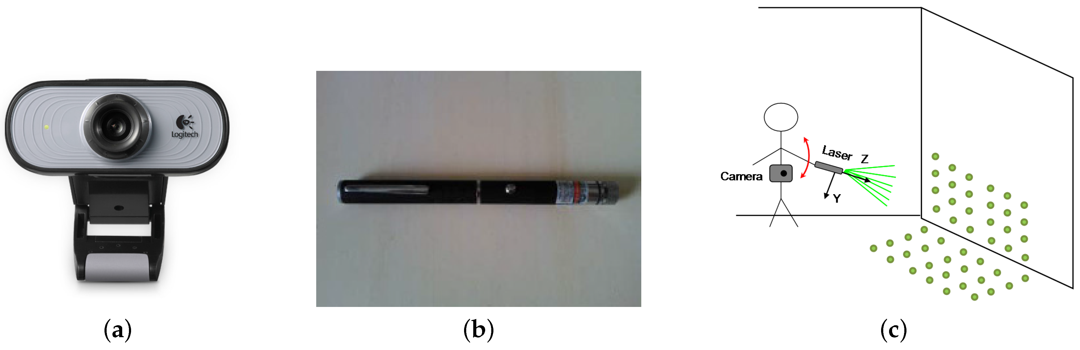
In this paper, we break with the rigidness of traditional structured light systems exploring a new configuration. We refer to this as non-rigid configuration. In our approach we use a wearable camera and a hand-held light emitter with free motion with respect to the camera. Both camera and light emitter are low-cost. In Figure 1 we show both devices and the configuration of the system. To the best of our knowledge only two previous works have considered a structured light system in non-rigid configuration. In [18] a wearable omnidirectional camera and a conic pattern light emitter are used and in [19] a scanning technique using a hand-held camera and a hand-held projector is presented. Our system differs from [18] and [19] in the use of a traditional perspective camera and a simple light emitter instead of expensive and heavy omnidirectional cameras or projectors with complex coding pattern.

Hence, in this work we present a novel, wearable, wide-baseline and low-cost structured light system in non-rigid configuration. Our proposal works in environments where the scene is formed by more than one planar surface. This assumption is reasonable in human-made environments in which the majority of the objects of interest are mainly composed of planes. We use the image of the light pattern acquired by the camera and a virtual image generated from the light emitter to perform the reconstruction of the scene. From this reconstruction we compute orientation and translation of the planar surfaces where the laser pattern has been projected. The 3D is obtained up to a scale factor, but with wide baseline because of the uncalibrated configuration proposed.

This work is a step towards the development of a human navigation assistance tool for visually-handicapped people. The development of new technologies in recent years has favored the appearance of powerful mobile devices that make everyday live of people easier, but these systems are usually developed considering people with normal abilities. However, they also have the potential to help people with special needs. For this reason, the long-term objective of this research is to provide a visually-handicapped person with a low-cost wearable system that helps him/her while moving inside a building. A wearable system must be flexible, light and affordable and must give the person the freedom to explore the environment without restrictions. Our system, in which the camera hangs from the person and the laser can be hand-held, can provide more flexibility and information than the common white cane for blind people. In order to help the person obtain the necessary information to move inside unknown indoor environments, which are mainly composed of planar surfaces, the system must be able to detect these planes and recover relevant information of the scene.

The remaining sections are organized as follows. In Section 2 the problem is formulated. In Section 3 the method to obtain the 3D information of a planar scene is presented. In Section 4 several simulations and experiments are shown. Finally, conclusions and remarks are given in Section 5.

2. Problem Definition

The problem that we tackle in this paper is the reconstruction of two or more planar surfaces in which the point-based pattern of the laser is projected and seen by the camera. Our approach uses two image projections: one image corresponds to the perspective camera and the second image is a virtual one obtained from the light emitter. In order to compute the reconstruction we need corresponding points in the images to compute the rotation and translation between camera and laser. To segment the 3D structure into planar surfaces, we use homographies and to compute the rotation and translation we use an algorithm based on homography decomposition. Therefore, in this section, we present the camera and laser model and the concept of homography that will be used throughout the paper.

2.1. Camera Model

We use a standard perspective camera assuming a pin-hole projection model. A point in space with coordinates $\mathbf{X}={[X,Y,Z]}^{\mathbf{T}}$ is mapped to the point on the image plane $(u,v)$ where a line joining the point $\mathbf{X}$ to the center of projection meets the image plane [2]. This projection is encapsulated in a projection matrix $\mathsf{P}\in {\mathrm{I}\mathrm{R}}^{3x4}$ composed by an intrinsic parameter matrix and an extrinsic one. Intrinsic parameters are focal distances $(f_x,f_y)$ and principal point coordinates $(C_x,C_y)$. Extrinsic parameters are rotation $\mathsf{R}$ and translation $\mathbf{t}$ between world and camera frames. Equation (1) defines mathematically this projection where the parameter s represents a scale factor.

$$\left[\begin{array}{c}u\\ v\\ s\end{array}\right]=\left[\begin{array}{ccc}{f}_x& 0& C_x\\ 0& f_y& C_y\\ 0& 0& 1\end{array}\right]\left[\begin{array}{cc}R& t\\ 0& 1\end{array}\right]\left[\begin{array}{c}X\\ Y\\ Z\\ 1\end{array}\right]$$

(1)

2.2. Laser Model

Our light emitter is a laser that projects a point-based pattern without any coding and generates synthetic features on the scene. In Figure 2 we show an image of the pattern. The projector can be modeled as a pin-hole camera since it can be conceptually regarded as an inverse camera projecting rays to the scene, with its z-axis pointing in the direction of the laser projection. Since we consider the laser as an inverse pin-hole camera it is possible to create a virtual perspective image from the projected pattern. Virtual images only require projective coordinates, therefore their image coordinates are relative to an scale. We propose to mesh the virtual image of the point-based pattern using a Delaunay triangulation [20] to facilitate some operations in our method. This meshed virtual image will be used subsequently to obtain the planes of the scene.

2.3. Homography

A planar surface in a 3D scene induces a projective transformation, called homography, that relates the projections in two views of any point belonging to the plane. As a mapping between a pair of image points in homogeneous coordinates, the planar homography is expressed by matrix $\mathsf{H}\in {\mathrm{I}\mathrm{R}}^{3x3}$. Since it is a general projective transformation defined up to scale (due to the scale ambiguity inherent to perspective projection), the homography matrix has 8 degrees of freedom. The homography mapping of one scene point provides two independent equations. Therefore, from a minimum number of four pairs of corresponding points the homography can be estimated linearly by solving the resulting system of equations [2]. Homographies have been extensively studied and different methods for their computation are available in the literature. They can be computed using lines instead of points in the presence of partial occlusions [21] and a second homography can be calculated using only three matches in an image pair [22].

3. Scene Reconstruction

In this section we propose an algorithm to reconstruct the 3D information of the planar surfaces that appear on the scene as well as the pose of the camera and the laser. In the first place, we extract the first plane of the scene using the concept of homography introduced before. Thanks to this extraction, we are able to obtain two solutions for the rotation and translation between the camera and the laser. Then, we segment the second and subsequent planes. This allows us to select the correct solution. Finally, we can compute the pose of the planes with respect to the camera using the previous information. We summarize this procedure in Algorithm 1.

Algorithm 1 Reconstruction of the scene

1: Extraction of the first plane (3.1). 2: Computation of two possible solutions for translation and rotation between camera and laser (3.2). 3: Segmentation of the second and subsequent planes and selection of the appropriate solution (3.3). 4: Calculation of the pose of all planes with respect to the camera (3.4).

3.1. First Plane Extraction

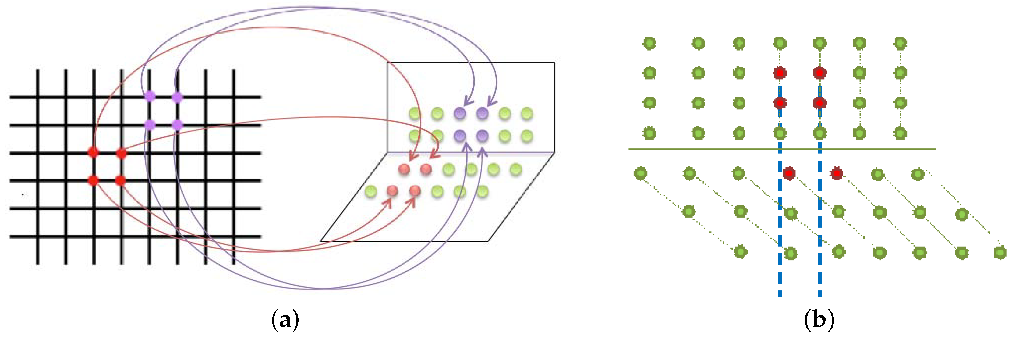
We extract the first plane of the scene calculating a homography. To find the homography that best fits the plane, we have to find all the points of the pattern that have been projected in it and their corresponding matchings in the virtual image. The following steps summarize the procedure to find such points. Recall that we compute a Delaunay triangulation with the points seen in both images.

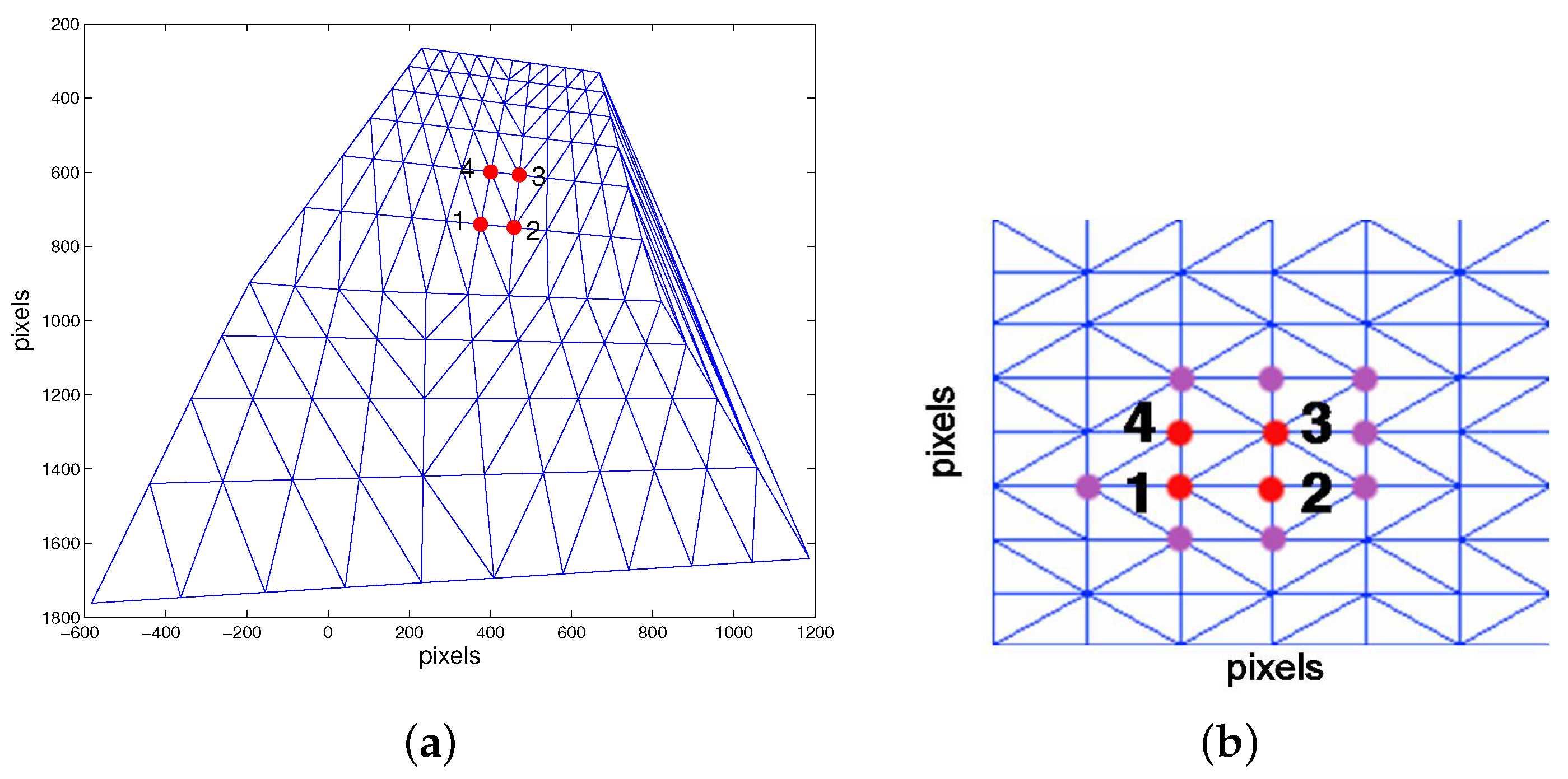
• Initial matching: four matches between the two images have to be established to initialize the homography. To do this, we proceed as follows. The first one is the central point of the pattern that we assume somehow coded in both images. In practice, this central point is easily recognizable as we discuss in the real experiments. The following are the nearest points to the horizontal and vertical lines defined by the previous ones counter-clockwise, i.e., the second is the nearest point to the horizontal line defined by the first one; the third, to the vertical line defined by the second one; and the fourth, to the horizontal line defined by the third one. An example of this initial matching can be seen in Figure 3. Any other selection can be done provided that the same relation between the points is maintained in both images.
• Neighbouring points search: we seek for the points that are neighbours to the points already matched. These are the points which form a triangle in the mesh with the matched points in both images. In Figure 3b the neighbouring points in the laser image are depicted in purple.
• Expansion of the homography: we apply for each neighbouring point in the image from the camera the transformation defined by the calculated homography and check if that point satisfies the correspondence in the laser image. At this point, the algorithm detects if the four initial points do not belong to the same plane because the calculated homography cannot be expanded. In such case, four different points have to be selected following the same order and relation in both images. This can be done since the central point of the pattern is known.
• Refinement of the homography: we compute a new homography with all the points which found valid correspondences in the previous step.

The last three steps are repeated until no neighbouring point finds a correspondence and, at that point, the segmentation of the first plane is completed.

3.2. Compute Rotation and Translation between Camera and Laser

The camera motion can be computed from the homography $\mathsf{H}$ obtained after the first plane extraction when the camera and laser are calibrated [23]. If the homography is calculated between image points and is expressed in pixels, we obtain an uncalibrated homography ${\mathsf{H}}_u$. However, if the intrinsic calibration parameters of camera and laser are known, a calibrated homography ${\mathsf{H}}_c$ can be computed as follows:

$${\mathsf{H}}_c={\mathsf{K}}_c^{-1}{\mathsf{H}}_u{\mathsf{K}}_l$$

(2)

where ${\mathsf{K}}_c$ and ${\mathsf{K}}_l$ are the calibration matrices of the camera and laser, respectively. This calibrated homography matrix encapsulates the relative location of the views and the unit normal of the scene plane in the following way:

$${\mathsf{H}}_{\mathsf{c}}=\lambda (\mathsf{R}+\mathbf{t}{\mathbf{n}}^{\mathsf{T}})$$

(3)

where $\mathsf{R}\in {\mathrm{I}\mathrm{R}}^{3x3}$ is the rotation matrix, $\mathbf{t}\in {\mathrm{I}\mathrm{R}}^3$ is the translation vector (scaled by the distance to the plane) between camera and laser and $\mathbf{n}\in {\mathrm{I}\mathrm{R}}^3$ is the unit normal of the plane. This homography is defined up to a scalar factor λ. In order to extract the laser pose from the homography matrix, it is necessary to compute the Euclidean homography ${\mathsf{H}}_e$ and to decompose it [24]. When computing the homography from image feature correspondences in homogeneous calibrated coordinates, we obtain a calibrated homography according to Equation (3).

As shown in [25], a 3x3 Euclidean homography matrix has its second largest singular value equal to one. Multiplying a matrix by a scale factor causes its singular values to be multiplied by the same factor. Then, for a given calibrated homography, we can obtain a unique Euclidean homography matrix (up to sign) by dividing the computed homography matrix by its second largest singular value. The sign ambiguity can be solved by employing the positive depth constraint. Computing the laser pose, $\mathsf{R}$ and $\mathbf{t}$, from the Euclidean homography, two physically valid solutions are obtained. A complete procedure for the computation of the laser pose from a calibrated homography is outlined in Algorithm 2.

Algorithm 2 Computation of laser pose from homography

1: Compute ${\mathsf{H}}_c={\mathsf{K}}_c^{-1}{\mathsf{H}}_u{\mathsf{K}}_l$ 2: Compute the SVD of ${\mathsf{H}}_c$ such that ${\mathsf{H}}_c\sim {\mathsf{H}}_e=\mathsf{U}\mathit{diag}({\lambda }_1,{\lambda }_2,{\lambda }_3)V^{\mathsf{T}}$ 3: Let $\alpha =\sqrt{\frac{{\lambda }_3^2-{\lambda }_2^2}{{\lambda }_3^2-{\lambda }_1^2}}$ and $\beta =\sqrt{\frac{{\lambda }_2^2-{\lambda }_1^2}{{\lambda }_3^2-{\lambda }_1^2}}$ 4: Writing $\mathsf{V}=[v_1,v_2,v_3]$, compute ${\mathbf{v}}_v=\alpha {\mathbf{v}}_1\pm \beta {\mathbf{v}}_3$ 5: Compute $\mathsf{R}=\left[\begin{array}{ccc}{\mathsf{H}}_e{\mathbf{v}}_v,& {\mathsf{H}}_e{\mathbf{v}}_2,& {\mathsf{H}}_e{\mathbf{v}}_v\times {\mathsf{H}}_e{\mathbf{v}}_2\end{array}\right]{\left[\begin{array}{ccc}{\mathbf{v}}_v,& {\mathbf{v}}_2,& {\mathbf{v}}_v\times {\mathbf{v}}_2\end{array}\right]}^T$ 6: Compute $\mathbf{t}={\mathsf{H}}_e\mathbf{n}-\mathsf{R}\mathbf{n}$ with $\mathbf{n}={\mathbf{v}}_v\times {\mathbf{v}}_2$

3.3. Segmentation of Second and Subsequent Planes

The segmentation of the second plane of the scene is performed in a similar way than the first one, calculating a homography. To do so, we need to establish four correspondences between both meshes to correctly initialize such homography (Figure 4a). We select two initial points as follows: we compute four straight lines from the first four initial points of the first plane and define four search areas: top, bottom, left and right. Between the points that have not been matched yet, we select the two closest to the straight lines that are situated in the same area (Figure 4b).

Due to the deformation of the pattern when it is projected on the second plane, there are several options to complete its initialization and cannot be carried out as for the first one. For this reason, we compute for each initialization hypothesis two homographies with rotation and translation fixed. Each one corresponds to one of the solutions obtained in the previous subsection for the rotation and translation between camera and laser. Now we introduce the calculation of these fixed-pose homographies.

3.3.1. Fixed-Pose Homography

Let ${\mathbf{p}}^A$ and ${\mathbf{p}}^B$ be the pair of selected corresponding points from the calibrated images; $\mathsf{R}$ and $\mathbf{t}$, the rotation and translation between camera and laser; $\mathbf{n}$ and d, the normal and the distance to the plane; s, a scale factor; and $\mathsf{H}$, the homography matrix. We have

$$s{\mathbf{p}}^B=\mathsf{H}{\mathbf{p}}^A=(\mathsf{R}+\mathbf{t}\frac{n^{\mathsf{T}}}{d}){\mathbf{p}}^A.$$

(4)

From Equation (4) we can formulate an equation system as follows:

$$\begin{array}{c}\left[\begin{array}{ccc}{t}_z{p}_x^A{p}_x^B-t_x{p}_x^A& t_z{p}_y^A{p}_x^B-t_x{p}_y^A& t_z{p}_x^B-t_x\\ t_z{p}_x^A{p}_y^B-t_y{p}_x^A& t_z{p}_y^A{p}_y^B-t_y{p}_y^A& t_z{p}_y^B-t_y\end{array}\right]\left[\begin{array}{c}\frac{n_x}{d}\\ \frac{n_y}{d}\\ \frac{n_z}{d}\end{array}\right]=\\ =\left[\begin{array}{c}{r}_{11}{p}_x^A+r_{12}{p}_y^A+r_{13}-r_{31}{p}_x^A{p}_x^B-r_{32}{p}_y^A{p}_x^B-r_{33}{p}_x^B\\ r_{21}{p}_x^A+r_{22}{p}_y^A+r_{23}-r_{31}{p}_x^A{p}_y^B-r_{32}{p}_y^A{p}_y^B-r_{33}{p}_y^B\end{array}\right],\end{array}$$

(5)

where

$$\mathsf{R}=\left[\begin{array}{ccc}{r}_{11}& r_{12}& r_{13}\\ r_{21}& r_{22}& r_{23}\\ r_{31}& r_{32}& r_{33}\end{array}\right],\mathbf{t}=\left[\begin{array}{c}{t}_x\\ t_y\\ t_z\end{array}\right],{\mathbf{p}}^A=\left[\begin{array}{c}{p}_x^A\\ p_y^A\end{array}\right],{\mathbf{p}}^B=\left[\begin{array}{c}{p}_x^B\\ p_y^B\end{array}\right],\frac{\mathbf{n}}{d}=\left[\begin{array}{c}\frac{n_x}{d}\\ \frac{n_y}{d}\\ \frac{n_z}{d}\end{array}\right]$$

(6)

According to Equation (5), the two pairs of corresponding points that we have already obtained are enough to solve the system. However, the rank of the system matrix is equal to two, resulting in an indefinite system. From a geometrical point of view, this is correct since two points define a beam of planes. Therefore, we have to include an additional correspondence from the initialization hypotheses being not collinear with the other two points. Using at least three pairs of corresponding points to solve Equation (5), the candidate normal to the second plane and the inverse distance to the plane for each hypothesis are obtained and using the calculated scaled normal we can finally compute each candidate homography with fixed pose according to Equation (3).

Eventually, only the correct initialization hypothesis together with the correct rotation and translation solution allows us to calculate a homography which expands along the second plane. This allows us to overcome the duplicity of solution for the rotation and translation.

To segment the subsequent planes, the relative pose between camera and laser is known thanks to the segmentation of the second plane. In the same way, a homography is calculated for each initialization hypothesis and we can find the correct homography because only the homography associated with the right initialization allows us to segment the plane. Note that this process is valid for every subsequent plane.

3.4. Planes Reconstruction

The last step is to compute rotation and translation of all the planes with respect to the camera. Assuming that the calibration matrices of the camera and the laser are known and with the rotation and translation between them calculated in the previous step, the projection matrices for both are computed. With the projection matrices and the correspondences established by the homographies, a triangulation process is used to compute the final reconstruction up to a scale factor.

4. Experiments

To verify the validity of the proposed method, we performed different experiments using simulated data and real images acquired with our non-rigid structured light system with laser in hand. Initially, we performed a sensitivity analysis with synthetic data. We added Gaussian noise to the image coordinates of the points and studied the influence of such noise. In the second place, we tested the reconstruction of a scene both in simulation and with the real system.

4.1. Simulations with Synthetic Data

We simulate a laser of 121 points with a field of view of 53 degrees. The camera has a resolution of 640 × 480 pixels with a field of view of 50 degrees in horizontal and 39 degrees in vertical. In order to evaluate the results of the simulations we define the laser translation error as the angle between estimated and real translation vectors. For rotation, we compute a rotation error matrix and put it on the axis-angle representation to use the angle as a single measure of the laser rotation error.

4.1.1. Sensitivity Analysis

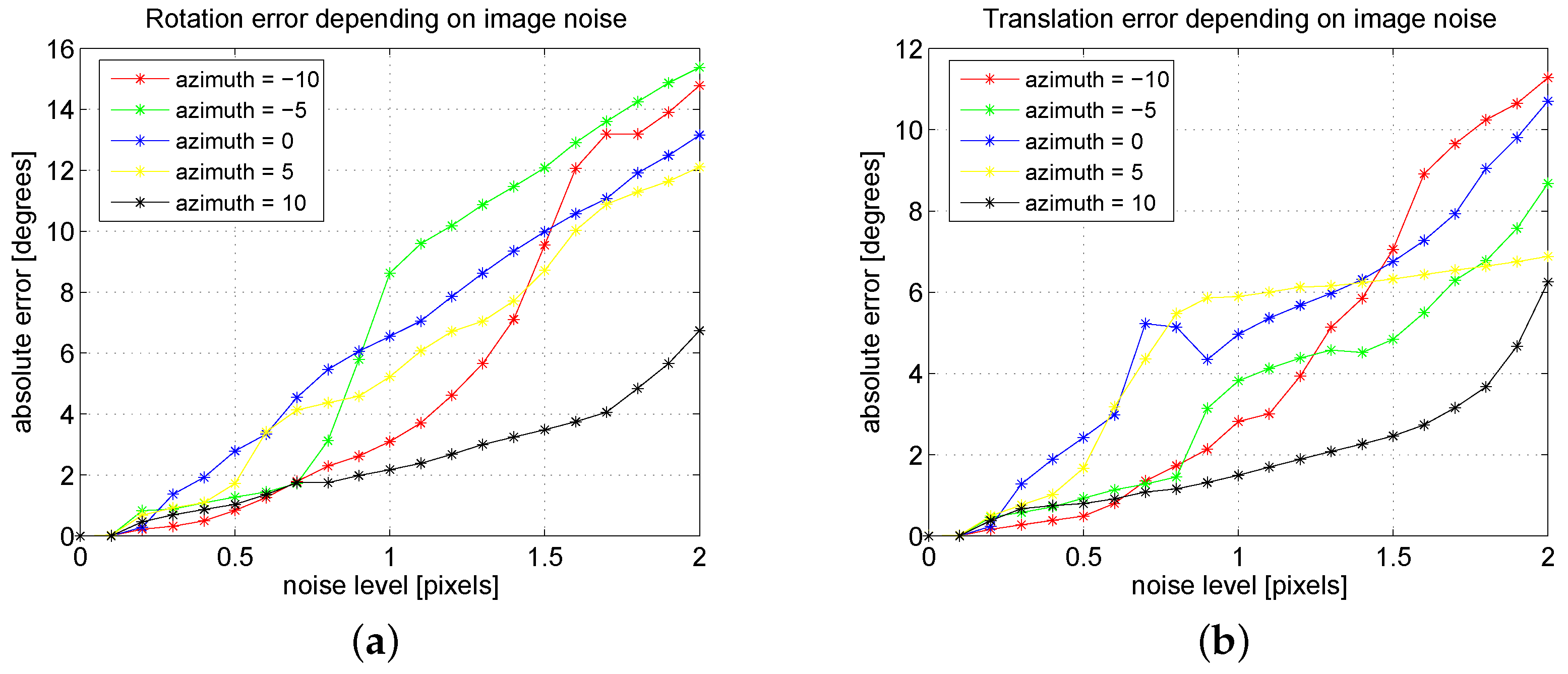
In the first place, we present the evolution of the rotation and translation error depending on the Gaussian noise introduced in the image points. We tested several configurations of the system in which both floor and wall planes were located one meter away from the camera. 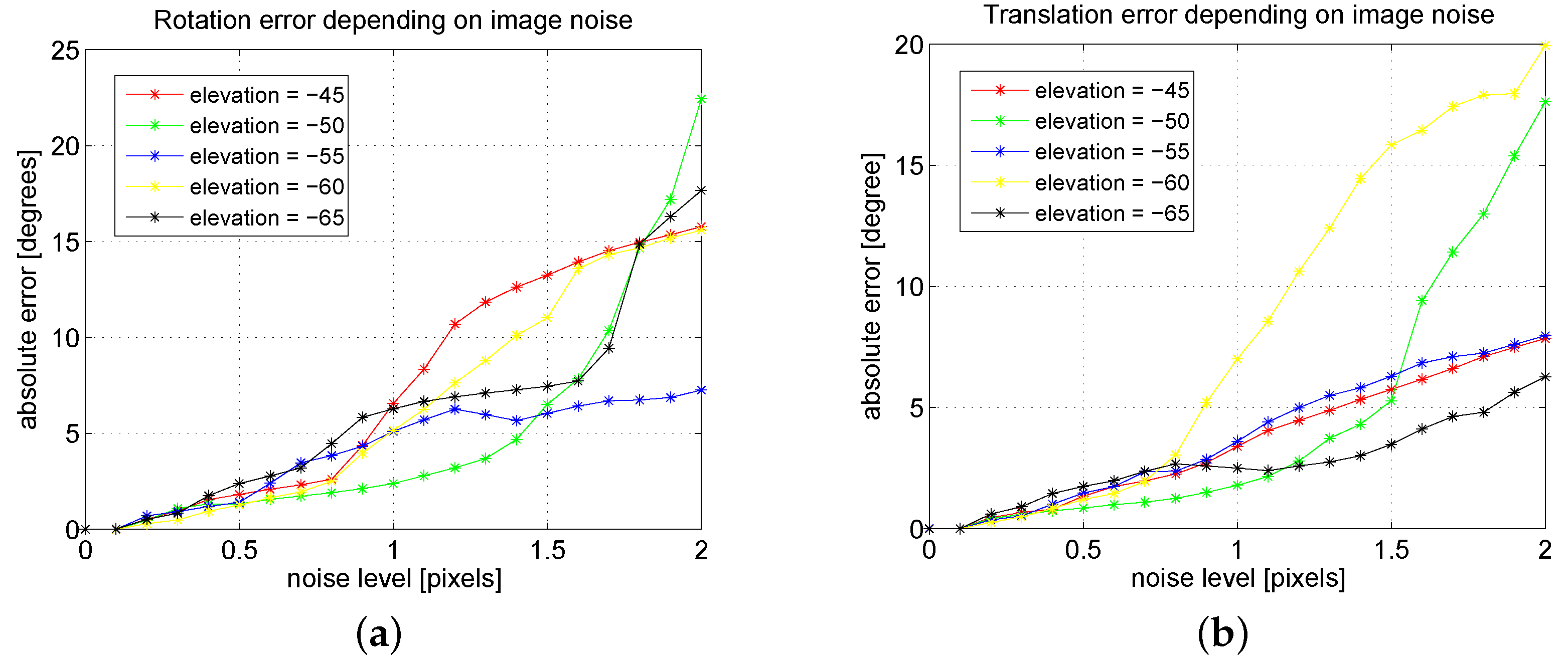In particular, we performed two scannings: a horizontal scanning in which we varied the azimuth angles of the light emitter from −10° to 10° in intervals of five degrees with a constant elevation of −60° (Figure 5), and a vertical scanning with elevation angles of the light emitter from −65° to −45° in intervals of five degrees with a constant azimuth of zero degrees (Figure 6).

In all the resulting configurations of these scannings, we added Gaussian noise of zero mean and standard deviation from 0 to 2 pixels in intervals of 0.1 pixels to the image point coordinates. The 121 points of the simulated pattern were seen in all the images. Results correspond to the mean errors of 1000 simulations for each configuration and each noise level. The results for the horizontal and vertical scannings are shown in Figure 5 and Figure 6, respectively. As expected, both rotation and translation errors grow with the image noise. However, the maximum errors in both variables are reasonable for the studied noise levels.

4.1.2. Reconstruction of a Simulated Scene

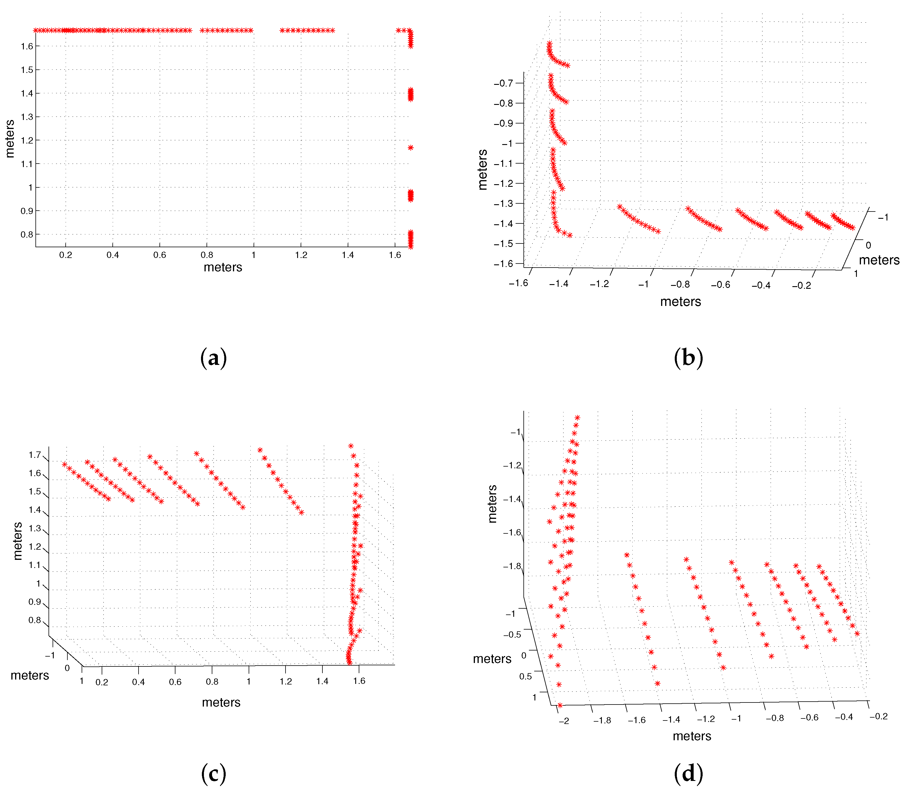
In the second place, we applied the proposed method to synthetic environments and we tested our algorithm in three different scenes: the first was composed by two orthogonal planes, the second contained three orthogonal planes and the third was formed by two non-orthogonal planes. We computed orientation and translation (up to scale) of the planes, that were located one meter away from the camera. The actual value for translation between camera and laser was (0.3, −0.3, 0.4) meters and for rotation, (−45 − 10, 3) degrees.

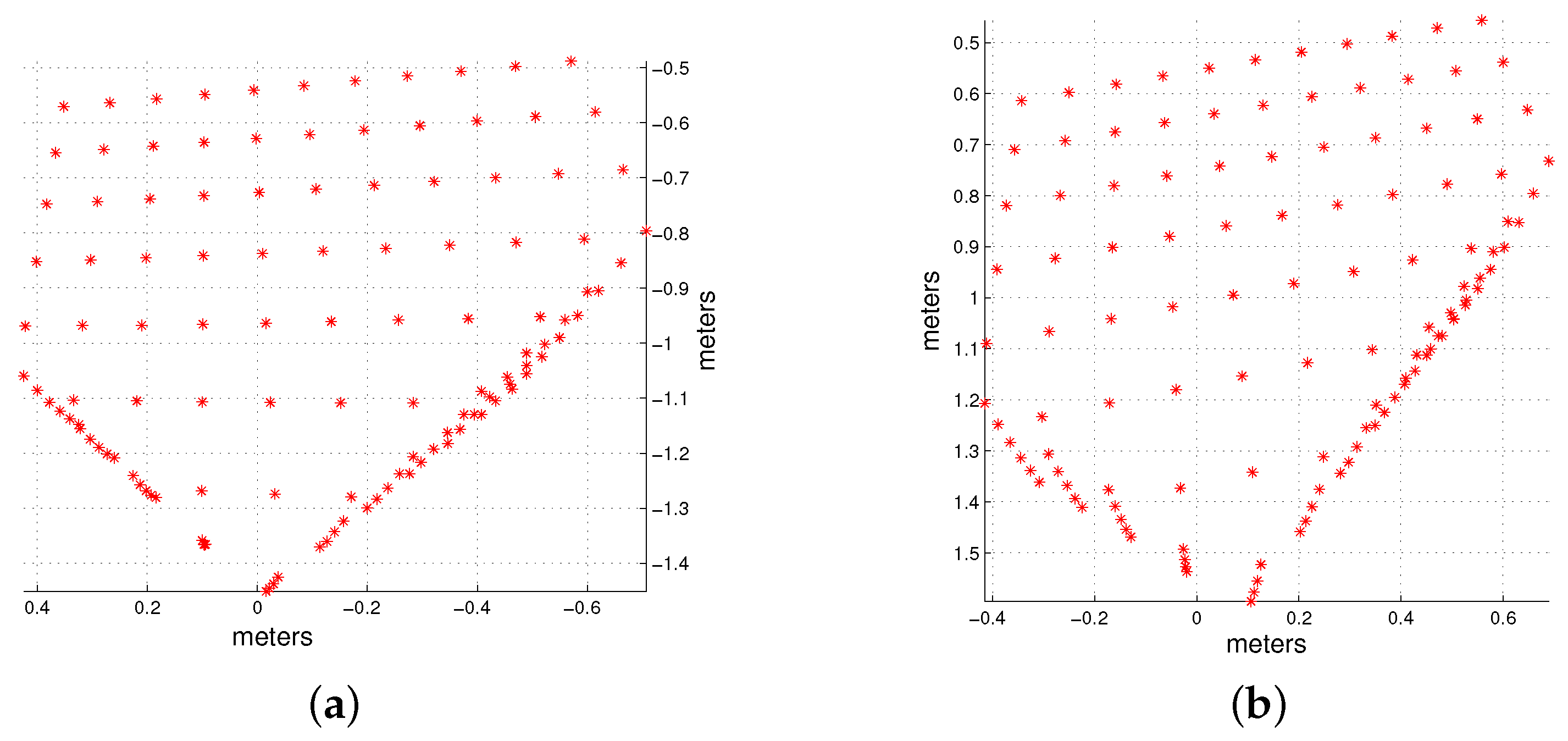
First, we show in Figure 7 the results of the reconstruction of the scene composed by two orthogonal planes. We added noise of varying mean to the image to study its effect upon the results. It can be seen that the obtained reconstruction of both planes is perfect when no noise is added to the point coordinates image (Figure 7a) and that the reconstruction deteriorates as more image noise is applied (Figure 7b–d).

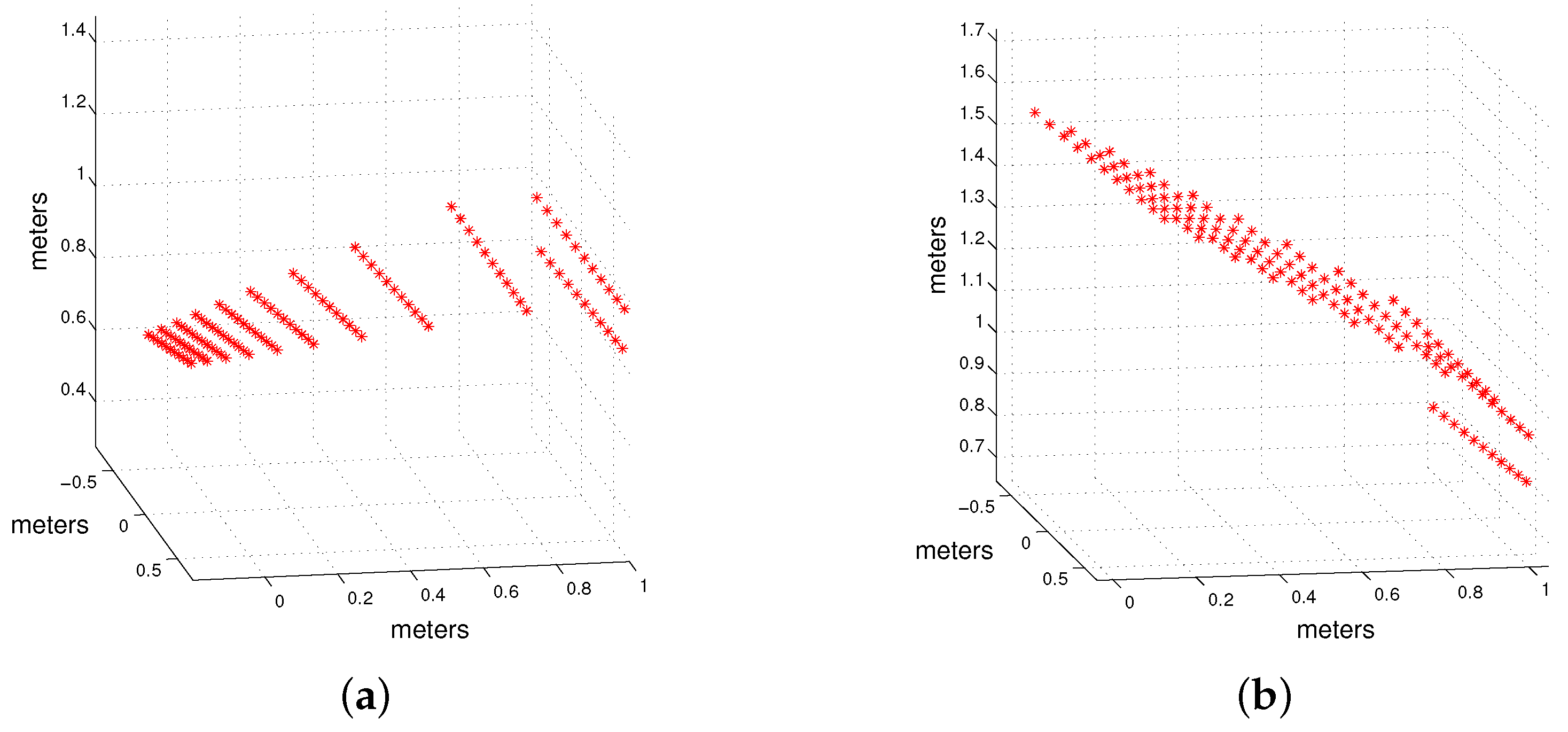
Second, we simulated three orthogonal planes and tested the algorithm (Figure 8). When working with three planes, the number of points projected onto each one is smaller than with two, and the fewer points per plane, the less accurate the reconstruction is. Although the reconstruction is not as accurate as for the case of two planes due to the lower number of points per plane, these results show that the three planes are reconstructed correctly. We also show in Figure 8 the effect of noise in the reconstruction of three planes. As for the case of two planes, when noise increases the reconstruction of the three planes deteriorates.

Finally, we performed experiments to confirm that the method is not affected by scenes in which planes are not orthogonal. We show in Figure 9 the reconstruction of two scenes in which the angle between planes is 75 and 120 degrees respectively. As can be seen the angle between planes does not influence the reconstruction. This was expected since we are not assuming perpendicularity at any point.

4.2. Real Experiments

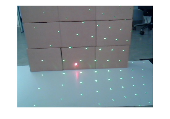
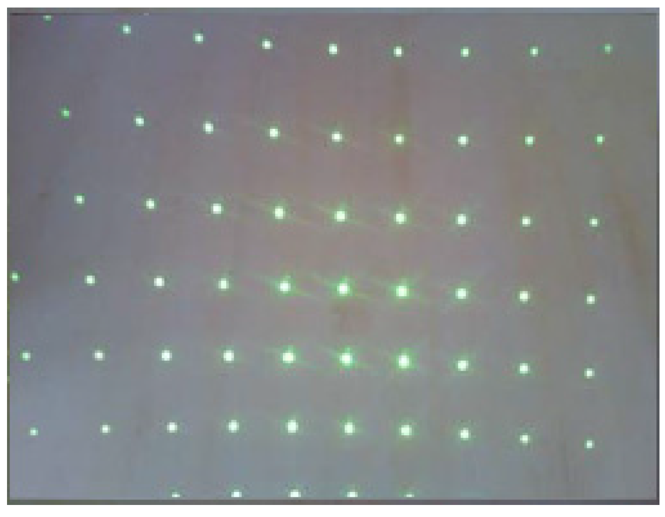
Real experiments were performed using our wearable non-rigid structured light system, which is composed of a perspective camera held on a belt and a low-cost laser in hand projecting a point-based pattern. The algorithm needs an intrinsic model projection of both camera and laser which can be computed separately. With respect to the camera we use the open-source software [26] which follows a standard calibration process. On the other hand, the method does not need an accurate calibration of the laser. A simple model assuming equidistant angles of projecting rays with the principal point in the image center has been considered. The angles between laser rays can be computed by knowing the distances between points which can be easily measured projecting to a fronto-parallel plane from known distance. We also need to define a common reference for laser and camera meshes. We use the central point of the pattern as origin of that reference. This point can be easily recognized. At this stage, we are using a red laser pointer coupled to the laser to mark the central point of the pattern. A more elaborated solution to obtain a common reference could be to use a non-symmetric pattern, a coded-light projector or even a specifically built projector developed for this application. Nevertheless, these alternatives would increase not only the cost of the system but also its weight in the case of coded-light projector.

To extract the point pattern and the red point, we used the HSI (Hue Saturation Intensity) space color since it is compatible with the vision physiology of human eyes [27] and its three components are independent. Using different thresholds in channels H and S we binarize the image and after smoothing, filtering and denoising operations the pattern and the red point can be extracted.

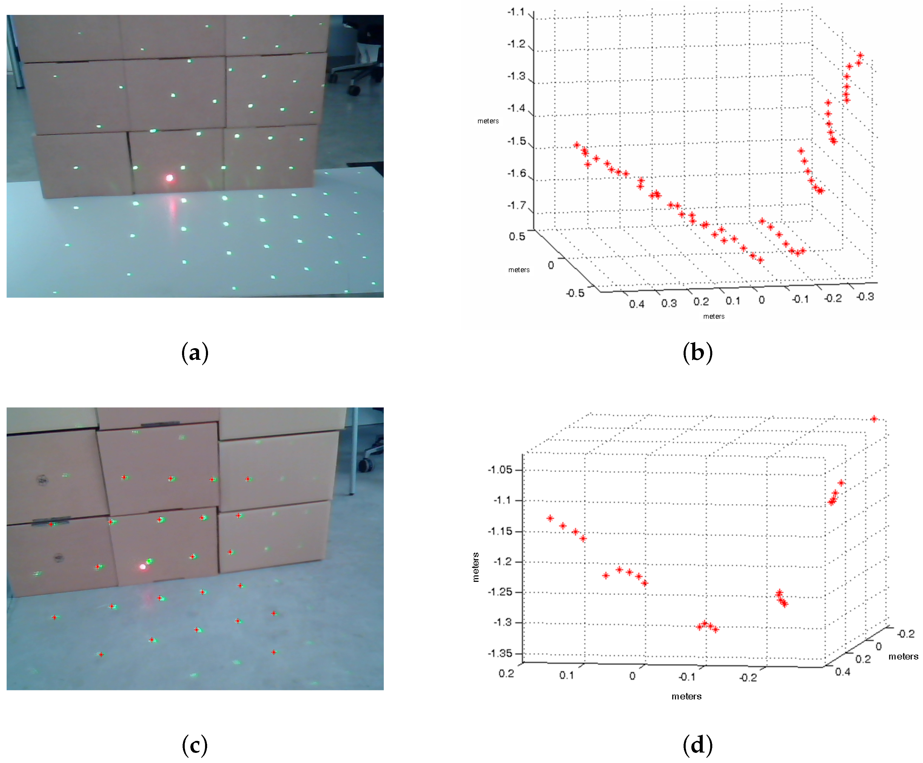
Once the light pattern and its central point are extracted from the image we apply our method to obtain the planes of the scene. The results for some different scenes are shown in Figure 10. To evaluate the accuracy of the reconstructed planes we compute the angle between their normal vectors. The results are shown in

Table 1. Angles between normal vectors for reconstructed planes.

	Normal Vector Plane 1	Normal Vector Plane 2	Angle between Planes
Experiment 1	(−0.50,0.55,−0.67) m	(0.25,0.88,0.39) m	85 degrees
Experiment 2	(−0.39,−0.55,−0.74) m	(0.18,0.87,0.46) m	86 degrees

. Although the reconstruction is not perfect due to the noise in the images, the reconstructed angles between the planes are near the actual value of 90 degrees.

We consider that these errors are acceptable since the goal is not to obtain accurate measurements of planes of a scene but to extract useful information to be interpreted by the person.

5. Conclusions

In this paper we have presented a new structured light system in non-rigid configuration which can be used as a personal assistance system. To recover the planes of a scene, this system only requires a single perspective image where the light pattern is present. To extract the planes, we have proposed the use of homographies and for rotation and translation calculation we have presented a method based on their decomposition where duplicity solutions problems have been solved. Our approach has shown good results on simulated and real data. In future work it would be interesting to develop a new system in which the intrinsic parameters of both camera and laser were not known. Related to this, we also expect to improve the current laser calibration. Another interesting research line is the improvement of the image processing in order to deal with more general illumination conditions. Finally, an open issue is to extend our approach to the case of non-planar scenes.