Article

Fisher Vector Coding for Covariance Matrix Descriptors Based on the Log-Euclidean and Affine Invariant Riemannian Metrics

1
Communications Department, Technical University of Cluj-Napoca, 71-73 Calea Dorobanților, 400114 Cluj-Napoca, Romania
2
Laboratoire IMS, Signal and Image group, Université de Bordeaux, CNRS, UMR 5218, 351 Cours de la Libération, 33400 Talence, France
*
Author to whom correspondence should be addressed.
Submission received: 29 April 2018 / Revised: 7 June 2018 / Accepted: 18 June 2018 / Published: 22 June 2018

Abstract

:
This paper presents an overview of coding methods used to encode a set of covariance matrices. Starting from a Gaussian mixture model (GMM) adapted to the Log-Euclidean (LE) or affine invariant Riemannian metric, we propose a Fisher Vector (FV) descriptor adapted to each of these metrics: the Log-Euclidean Fisher Vectors (LE FV) and the Riemannian Fisher Vectors (RFV). Some experiments on texture and head pose image classification are conducted to compare these two metrics and to illustrate the potential of these FV-based descriptors compared to state-of-the-art BoW and VLAD-based descriptors. A focus is also applied to illustrate the advantage of using the Fisher information matrix during the derivation of the FV. In addition, finally, some experiments are conducted in order to provide fairer comparison between the different coding strategies. This includes some comparisons between anisotropic and isotropic models, and a estimation performance analysis of the GMM dispersion parameter for covariance matrices of large dimension.

1. Introduction

In supervised classification, the goal is to tag an image with one class name based on its content. In the beginning of the 2000s, the leading approaches were based on feature coding. Among the most employed coding-based methods, there are the bag of words model (BoW) [1], the vector of locally aggregated descriptors (VLAD) [2,3], the Fisher score (FS) [4] and the Fisher vectors (FV) [5,6,7]. The success of these methods is based on their main advantages. First, the information obtained by feature coding can be used in a wide variety of applications, including image classification [5,8,9], text retrieval [10], action and face recognition [11], etc. Second, combined with powerful local handcrafted features, such as SIFT, they are robust to transformations like scaling, translation, or occlusion [11].
Nevertheless, in 2012, the ImageNet Large Scale Visual Recognition Challenge has shown that Convolutional Neural Networks [12,13] (CNNs) can outperform FV descriptors. Since then, in order to take advantage of both worlds, some hybrid classification architectures have been proposed to combine FV and CNN [14]. For example, Perronnin et al. have proposed to train a network of fully connected layers on the FV descriptors [15]. Another hybrid architecture is the deep Fisher network composed by stacking several FV layers [16]. Some authors have proposed to extract convolutional features from different layers of the network, and then to use VLAD or FV encoding to encode features into a single vector for each image [17,18,19]. These latter features can also be combined with features issued from the fully connected layers in order to improve the classification accuracy [20].
At the same time, many authors have proposed to extend the formalism of encoding to features lying in a non-Euclidean space. This is the case of covariance matrices that have already demonstrated their importance as descriptors related to array processing [21], radar detection [22,23,24,25], image segmentation [26,27], face detection [28], vehicle detection [29], or classification [11,30,31,32], etc. As mentioned in [33], the use of covariance matrices has several advantages. First, they are able to merge the information provided by different features. Second, they are low dimensional descriptors, independent of the dataset size. Third, in the context of image and video processing, efficient methods for fast computation are available [34].
Nevertheless, since covariance matrices are positive definite matrices, conventional tools developed in the Euclidean space are not well adapted to model the underlying scatter of the data points which are covariance matrices. The characteristics of the Riemannian geometry of the space P m of m × m symmetric and positive definite (SPD) matrices should be considered in order to obtain appropriate algorithms. The aim of this paper is to introduce a unified framework for BoW, VLAD, FS and FV approaches, for features being covariance matrices. In the recent literature, some authors have proposed to extend the BoW and VLAD descriptors to the LE and affine invariant Riemannian metrics. This yields to the so-called Log-Euclidean bag of words (LE BoW) [33,35], bag of Riemannian words (BoRW) [36], Log-Euclidean vector of locally aggregated descriptors (LE VLAD) [11], extrinsic vector of locally aggregated descriptors (E-VLAD) [37] and intrinsic Riemannian vector of locally aggregated descriptors (RVLAD) [11]. All these approaches have been proposed by a direct analogy between the Euclidean and the Riemannian case. For that, the codebook used to encode the covariance matrix set is the standard k-means algorithm adapted to the LE and affine invariant Riemannian metrics.
Contrary to the BoW and VLAD-based coding methods, a soft codebook issued from a Gaussian mixture model (GMM) should be learned for FS or FV encoding. This paper aims to present how FS and FV can be used to encode a set of covariance matrices [38]. Since these elements do not lie on an Euclidean space but on a Riemannian manifold, a Riemannian metric should be considered. Here, two Riemannian metrics are used: the LE and the affine invariant Riemannian metrics. To summarize, we provide four main contributions:
  • First, based on the conventional multivariate GMM, we introduce the log-Euclidean Fisher score (LE FS). This descriptor can be interpreted as the FS computed on the log-Euclidean vector representation of the covariance matrices set.
  • Second, we have recently introduced a Gaussian distribution on the space P m : the Riemannian Gaussian distribution [39]. This latter allows the definition of a GMM on the space of covariance matrices and an Expectation Maximization (EM) algorithm can hence be considered to learn the codebook [32]. Starting from this observation, we define the Riemannian Fisher score (RFS) [40] which can be interpreted as an extension of the RVLAD descriptor proposed in [11].
  • The third main contribution is to highlight the impact of the Fisher information matrix (FIM) in the derivation of the FV. For that, the Log-Euclidean Fisher Vectors (LE FV) and the Riemannian Fisher Vectors (RFV) are introduced as an extension of the LE FS and the RFS.
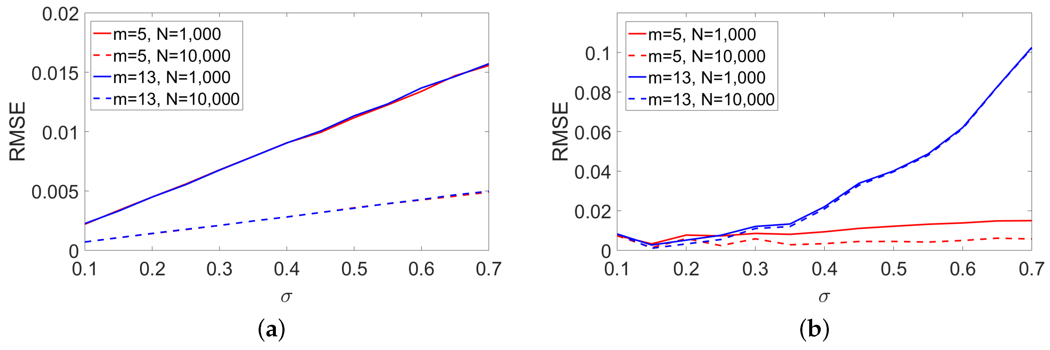
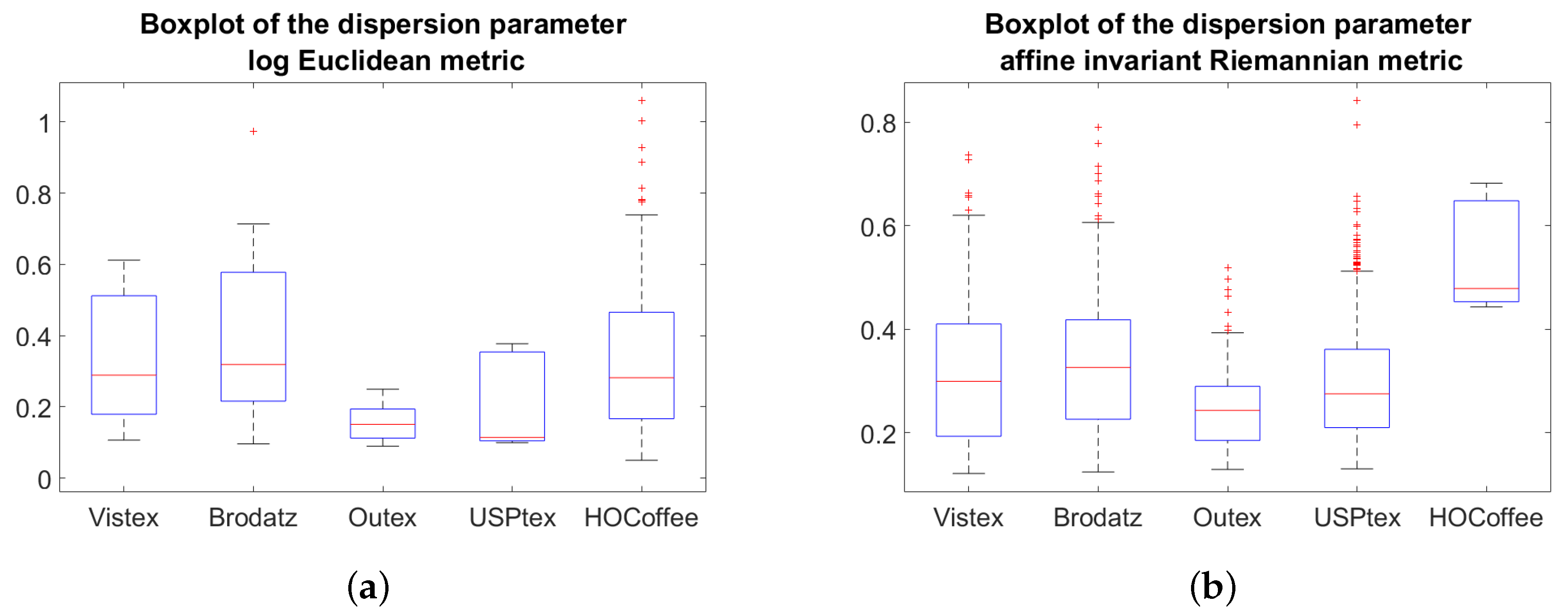
  • Fourth, all these coding methods will be compared on two image processing applications consisting of texture and head pose image classification. Some experiments will also be conducted in order to provide fairer comparison between the different coding strategies. It includes some comparisons between anisotropic and isotropic models. An estimation performance analysis of the dispersion parameter for covariance matrices of large dimension will also be studied.
As previously mentioned, hybrid architectures can be employed to combine FV with CNN. The adaptation of the proposed FV descriptors to these architecture is outside the scope of this paper but will remain one of the perspective of this work.
The paper is structured as follows. 
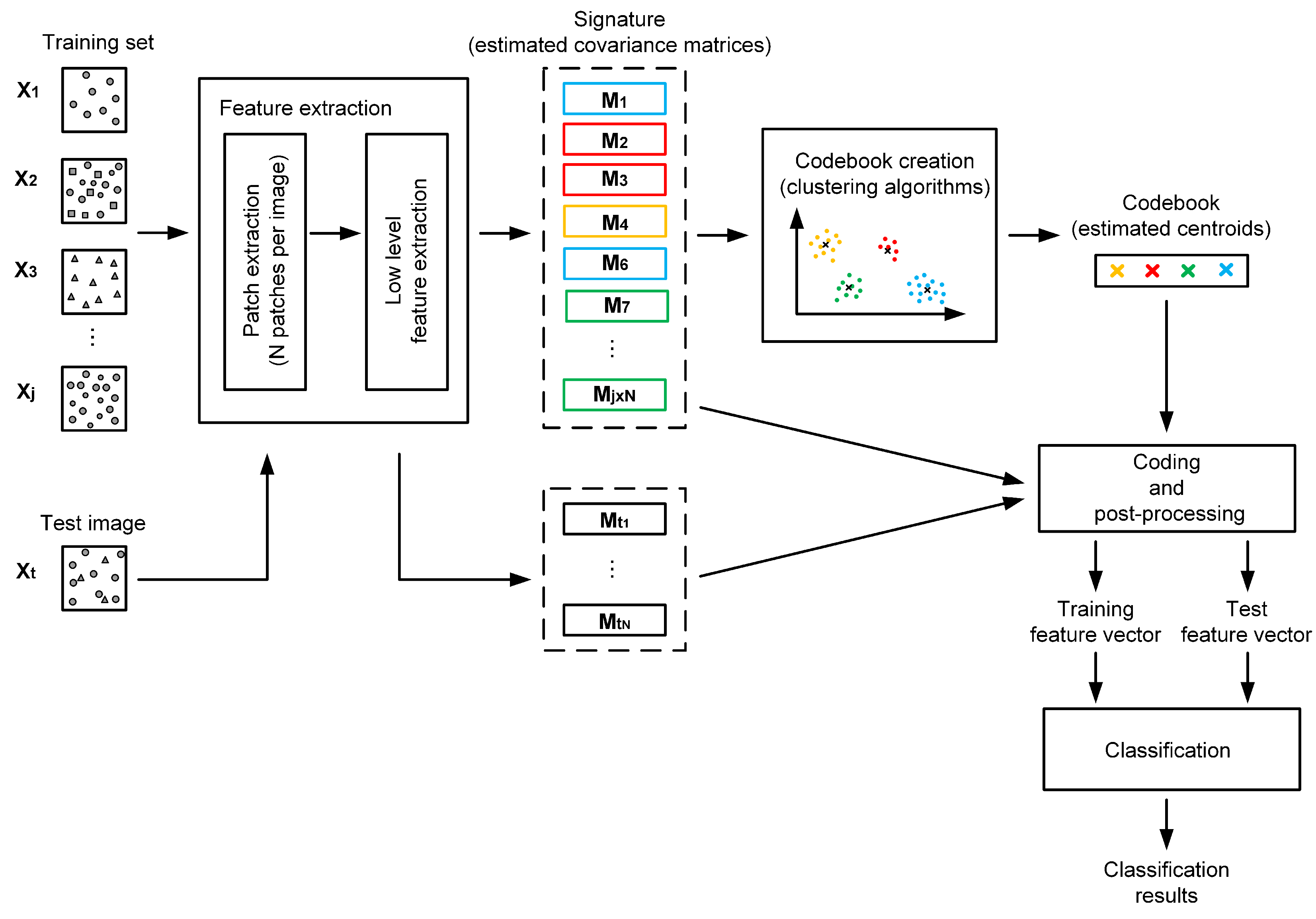
Section 2 introduces the workflow presenting the general idea of feature coding-based classification methods. Section 3 presents the codebook generation on the manifold of SPD covariance matrices. Section 4 introduces a theoretical study of the feature encoding methods (BoW, VLAD, FS and FV) based on the LE and affine invariant Riemannian metrics. 
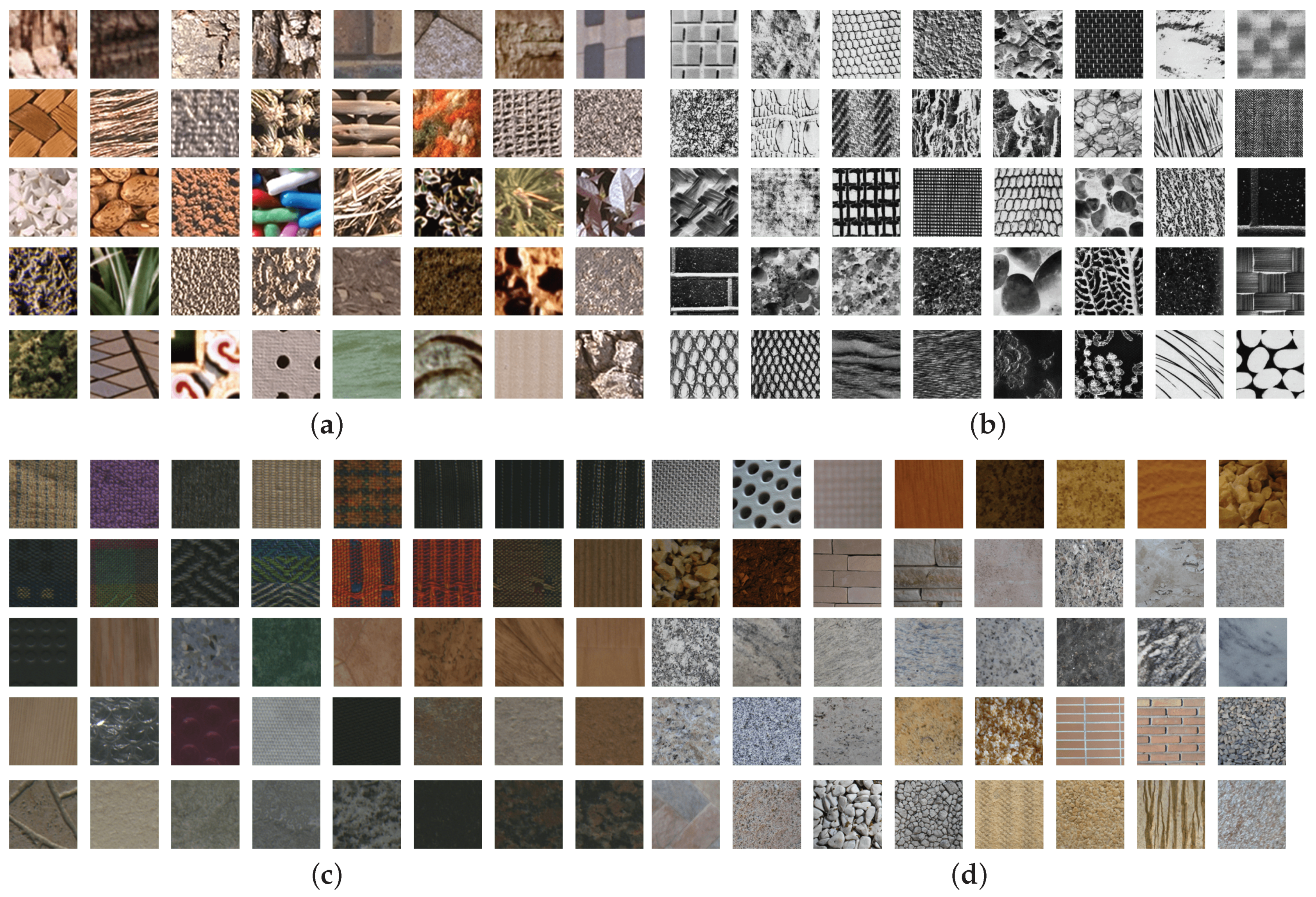
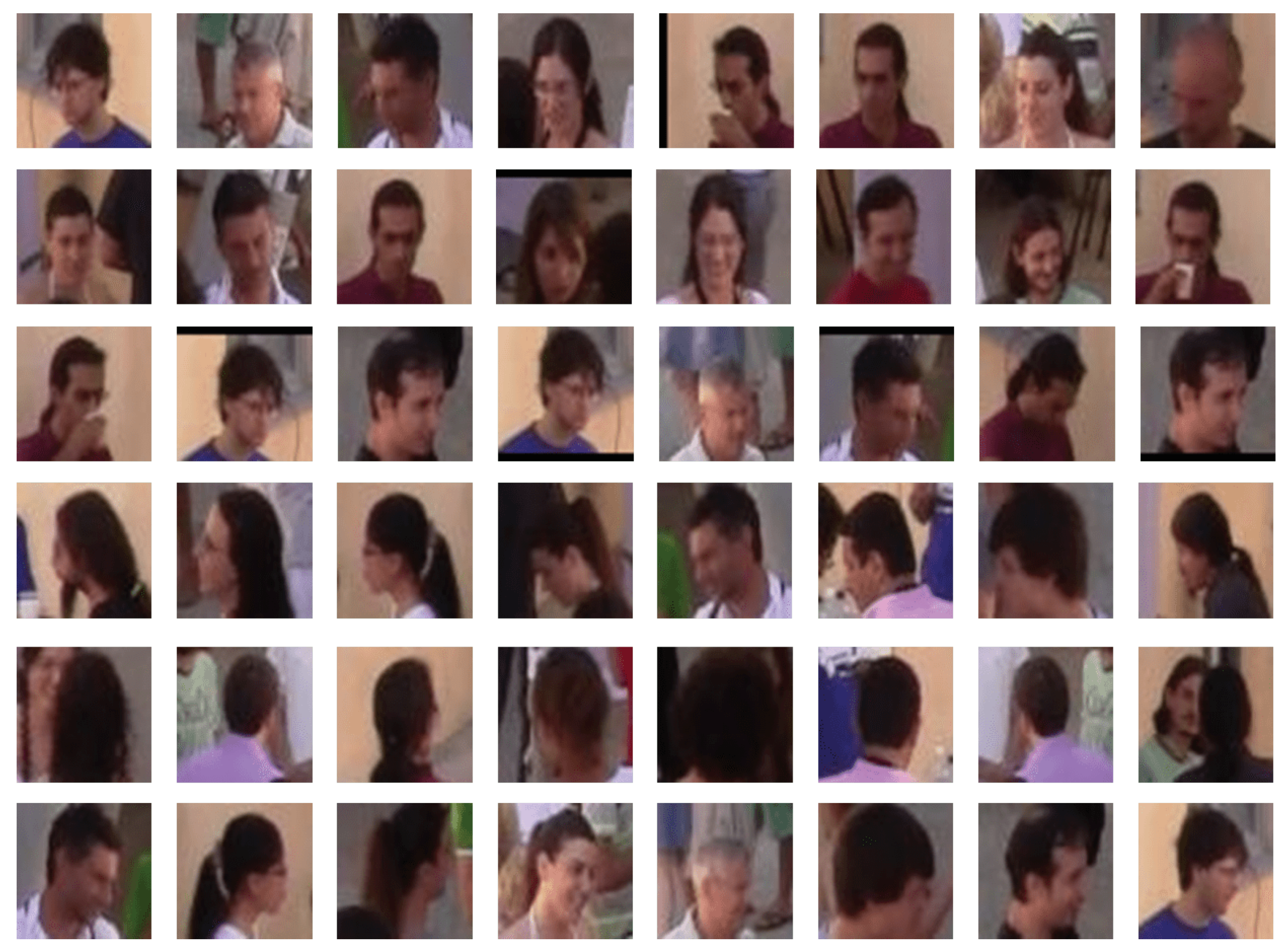
Section 5 shows two applications of these descriptors to texture and head pose image classification. In addition, finally, Section 6 synthesizes the main conclusions and perspectives of this work.

2. General Framework

The general workflow is presented in Figure 1 and it consists of the following steps:
  • Patch extraction is the starting step of the classification algorithm. At the beginning, the images are divided in patches, either in a dense way, by means of fixed grids, or in a non-dense way, based on representative points such as SIFT for example.
  • A low level feature extraction step is then applied in order to extract some characteristics (such as spatial gradient components). These low-level handcrafted features capture the information contained in each patch.
  • The covariance matrix of these features are then computed. As a result, each image is represented as a set of covariance matrices which compose the signature of an image.
  • The codebook generation starts from the previously extracted covariance matrices. The purpose of this step is to identify the features containing the significant information. Usually, this procedure is performed by means of clustering algorithms, such as the k-means or expectation-maximization (EM) algorithm. Knowing that the features are covariance matrices, one of the following approaches can be chosen. The first one considers the LE metric. It consists of projecting the covariance matrices in the LE space [33,35] and then standard clustering algorithms for multivariate Gaussian distributions are used. The second approach considers the affine invariant Riemannian metric to measure the similarity between two covariance matrices. In this context, the conventional k-means or EM algorithm should be readapted to this metric [11,36,40]. For both approaches, the dataset is partitioned into a predefined number of clusters, each of them being described by parameters, such as the cluster’s centroid, the dispersion and the associated weight. The obtained features are called codewords and they are grouped in a codebook, also called a dictionary.
  • Feature encoding is based on the created codebook and it consists in projecting the extracted covariance matrices onto the codebook space. For this purpose, approaches like BoW, VLAD and FV can be employed, for both the LE and affine invariant Riemannian metrics. According to [41], these are global coding strategies, that describe the entire set of features, and not the individual ones. Essentially, this is accomplished using probability density distributions to model the feature space. More precisely, they can be viewed either as voting-based methods depending on histograms, or as Fisher coding-based methods by using Gaussian mixture models adapted to the considered metric [39,42].
  • Post-processing is often applied after the feature encoding step, in order to minimize the influence of background information on the image signature [6] and to correct the independence assumption made on the patches [7]. Therefore, two types of normalization are used, namely the power [7] and 2 [6] normalizations.
  • Classification is the final step, achieved by associating the test images to the class of the most similar training observations. In practice, algorithms such as k-nearest neighbors, support vector machine or random forest can be used.
As shown in Figure 1, the codebook generation along with the feature encoding are the two central steps in this framework. The next two sections present a detailed analysis of how these steps are adapted to covariance matrix features.

3. Codebook Generation in P m

This section focuses on the codebook generation. At this point, the set of extracted low-level features, i.e., the set of covariance matrices, is used in order to identify the ones embedding the set’s significant characteristics. In this paper, two metrics are considered to compute the codebook which are respectively the LE and the affine invariant Riemannian metric. The next two subsections describe these two strategies.

3.1. Log-Euclidean Codebook

Let M = { M n } n = 1 : N , with M n P m , be a sample of N training SPD matrices of size m × m . The LE codebook is obtained by considering the LE metric as similarity measure between two covariance matrices. For such a purpose, each training covariance matrix M n is first mapped on the LE space by applying the matrix logarithm M n L E = log M n [33,43,44]. Next, a vectorization operator is applied to obtain the LE vector representation. To sum up, for a given SPD matrix M , its LE vector representation, m R m ( m + 1 ) 2 , is defined as m = Vec ( log ( M ) ) where Vec is the vectorization operator defined as:
Vec ( X ) = X 11 , 2 X 12 , , 2 X 1 m , X 22 , 2 X 23 , , X m m ,
with X i j the elements of X .
Once the SPD matrices are mapped on the LE metric space, all the conventional algorithms developed on the Euclidean space can be considered. In particular, the LE vector representation of M , i.e., { m n } n = 1 : N , can be assumed to be independent and identically distributed (i.i.d.) samples from a mixture of K multivariate Gaussian distributions, whose probability density function is
p ( m n | θ ) = k = 1 K ϖ k p ( m n | m ¯ k , Σ k )
where θ = { ( ϖ k , m ¯ k , Σ k ) 1 k K } is the parameter vector. For each cluster k, ϖ k represent the mixture weight, m ¯ k the mean vector and M k the covariance matrices. It yields:
p ( m | θ k ) = 1 ( 2 π ) m 2 | Σ k | 1 2 exp 1 2 ( m m ¯ k ) T Σ k 1 ( m m ¯ k ) ,
where ( · ) T is the transpose operator, | · | is the determinant, m ¯ k R m ( m + 1 ) 2 , Σ k P m ( m + 1 ) / 2 and ϖ k R . In addition, the covariance matrix is assumed to be diagonal, i.e., σ k 2 = diag ( Σ k ) R m ( m + 1 ) 2 is the variance vector. For such a model, the classical k-means or EM algorithm can be applied to estimate the mixture parameters. The estimated parameters of each mixture component ( m ¯ k , σ k 2 and ϖ k ) represent the codewords and the set composed by the K codewords gives the LE codebook.

3.2. New Riemannian Codebook

In this section, we present the construction of the Riemannian codebook which is based on the affine invariant Riemannian metric. We recall some properties of the manifold of SPD matrices and introduce the Riemannian Gaussian mixture model.

3.2.1. Riemannian Geometry of the Space of SPD Matrices

The space P m of m × m real SPD matrices M satisfies the following conditions:
M M T = 0
and
x T M x > 0 ,
x R m and x 0 .
In this space, the Rao-Fisher metric defines a distance, called the Rao’s geodesic distance [45,46], given by the length of the shortest curve connecting two points in P m . Mathematically, this definition can be stated as follows [32]. Let M 1 , M 2 be two points in P m and c : [ 0 , 1 ] P m a differentiable curve, with c ( 0 ) = M 1 and c ( 1 ) = M 2 . Thus, the length of curve c, denoted by L ( c ) is defined as:
L ( c ) = 0 1 d c d t d t .
The geodesic distance d : P m × P m R + between M 1 and M 2 is the infimum of L ( c ) with respect to all differentiable curves c. Based on the properties of Rao-Fisher metric, it has been shown that the unique curve γ fulfilling this condition is [45,46]:
γ ( t ) = M 1 1 2 M 1 1 2 M 2 M 1 1 2 t M 1 1 2 ,
called the geodesic connecting M 1 and M 2 . Moreover, the distance between two points in P m can be expressed as [47]:
d 2 ( M 1 , M 2 ) = tr log ( M 1 1 2 M 2 M 1 1 2 ] 2 = i = 1 m ( ln λ i ) 2 ,
with λ i , i = 1 , , m being the eigenvalues of M 1 1 M 2 .
The affine invariant Riemannian (Rao-Fisher) metric can be also used to define the Riemannian volume element [45]:
d v ( M ) = | M | m + 1 2 i j d M i j .
For each point on the manifold M 1 P m , the tangent space at M 1 , denoted by T M 1 can be defined. This space contains the vectors V T that are tangent to all possible curves passing through M 1 . The correspondence between a point on the manifold and its tangent space can be achieved by using two operators: the Riemannian exponential mapping and the Riemannian logarithm mapping [48,49].
More precisely, the Riemannian exponential mapping for a point M 1 P m and the tangent vector V T is given by [48,49]:
M 2 = Exp M 1 ( V T ) = M 1 1 2 exp M 1 1 2 V T M 1 1 2 M 1 1 2 ,
where exp ( · ) is the matrix exponential. By this transformation, the tangent vector V T can be mapped on the manifold.
Further on, the inverse of the Riemannian exponential mapping is the Riemannian logarithm mapping. For two points M 1 , M 2 P m , this operator is given by [48,49]:
V T = Log M 1 ( M 2 ) = M 1 1 2 log M 1 1 2 M 2 M 1 1 2 M 1 1 2 ,
where log ( · ) is the matrix logarithm. In practice, this operation gives the tangent vector V T , by transforming the geodesic γ in a straight line in the tangent space. In addition, the geodesic’s length between M 1 and M 2 is equal to the norm of the tangent vector V T .

3.2.2. Mixture of Riemannian Gaussian Distribution

Riemannian Gaussian model
To model the space P m of SPD covariance matrices, a generative model has been introduced in [39,42]: the Riemannian Gaussian distribution (RGD). For this model, the probability density function with respect to the Riemannian volume element given in (9) is defined as follow [39,42]:
p ( M n | M ¯ , σ ) = 1 Z ( σ ) exp d 2 ( M n , M ¯ ) 2 σ 2 ,
where M ¯ and σ are the distribution parameters, representing respectively the central value (centroid) and the dispersion. d ( · ) is the Riemannian distance given in (8) and Z ( σ ) is a normalization factor independent of M ¯ [39,50].
Z ( σ ) = 8 m ( m 1 ) 4 π m 2 / 2 m ! Γ m ( m / 2 ) R m e r 2 2 σ 2 i < j sinh | r i r j | 2 i = 1 m d r i
with Γ m the multivariate Gamma function [51]. In practice, for m = 2 , the normalization factor admits a closed-form expression [32], while for m > 2 the normalization factor can be computed numerically as the expectation of the product of sinh functions with respect to the multivariate normal distribution N ( 0 , σ 2 I m ) [39]. Afterwards, a cubic spline interpolation can be used to smooth this function [52].
Mixture model for RGDs
As for the LE codebook, a generative model is considered for the construction of the Riemannian codebook. For the former, a mixture of multivariate Gaussian distribution was considered since the SPD matrices were projected on the LE space. For the construction of the Riemannian codebook, we follow a similar approach by considering that M = { M n } n = 1 : N , are i.i.d. samples from a mixture of K RGDs. In this case, the likelihood of M is given by:
p ( M | θ ) = n = 1 N p ( M n | θ ) = n = 1 N k = 1 K ϖ k p ( M n | M ¯ k , σ k ) ,
where p ( M n | M ¯ k , σ k ) is the RGD defined in (12) and θ = { ( ϖ k , M ¯ k , σ k ) 1 k K } is the parameter vector containing the mixture weight ϖ k , the central value M ¯ k and the dispersion parameter σ k .
Once estimated, the parameters of each mixture component represent the codewords, and the set of all K codewords gives the Riemannian codebook. Regarding the estimation, the conventional intrinsic k-means clustering algorithm can be considered [36,53]. Nevertheless, it implies the homoscedasticity assumption, for which the clusters have the same dispersion. To relax this assumption, we consider in the following the maximum likelihood estimation with the expectation maximization algorithm defined in [32].
Maximum likelihood estimation
First, let us consider the following two quantities that are defined for each mixture component k, k = 1 , , K :
γ k ( M n , θ ) = ϖ k × p ( M n | M ¯ k , σ k ) j = 1 K ϖ j × p ( M n | M ¯ j , σ j )
and
n k ( θ ) = n = 1 N γ k ( M n , θ ) .
Then, the estimated parameters θ ^ = { ( ϖ ^ k , M ¯ ^ k , σ ^ k ) 1 k K } are iteratively updated based on the current value of θ ^ :
  • The estimated mixture weight ϖ ^ k is given by:
    ϖ ^ k = n k ( θ ^ ) k = 1 K n k ( θ ^ ) ;
  • The estimated central value M ¯ ^ k is computed as:
    M ¯ ^ k = arg min M n = 1 N γ k ( M n , θ ^ ) d 2 ( M , M n ) ;
    In practice, (18) is solved by means of a gradient descent algorithm [54].
  • The estimated dispersion σ ^ k is obtained as:
    σ ^ k = Φ n k 1 ( θ ) × n = 1 N ω k ( M n , θ ^ ) d 2 ( M ¯ ^ k , M n ) ,
    where Φ is the inverse function of σ σ 3 × d d σ log Z ( σ ) .
Practically, the estimation procedure is repeated for a fixed number of iterations, or until convergence, that is until the estimated parameters remain almost stable for successive iterations. Moreover, as the estimation with the EM algorithm depends on the initial parameter setting, the EM algorithm is run several times (10 in practice) and the best result is kept (i.e., the one maximizing the log-likelihood criterion).
Based on the extracted (LE or Riemannian) codebook, the next section presents various strategies to encode a set of SPD matrices. These approaches are based whether on the LE metric or on the affine invariant Riemannian metric. In the next section, three kinds of coding approaches are reviewed, namely the bag of words (BoW) model, the vector of locally agregated descriptors (VLAD) [2,3] and the Fisher vectors (FV) [5,6,7]. Here, the main contribution is the proposition of coding approaches based on the FV model: the Log-Euclidean Fisher vectors (LE FV) and the Riemannian Fisher vectors (RFV) [40].

4. Feature Encoding Methods

Given the extracted codebook, the purpose of this part is to project the feature set of SPD matrices onto the codebook elements. In other words, the initial feature set is expressed using the codewords contained in the codebook. 
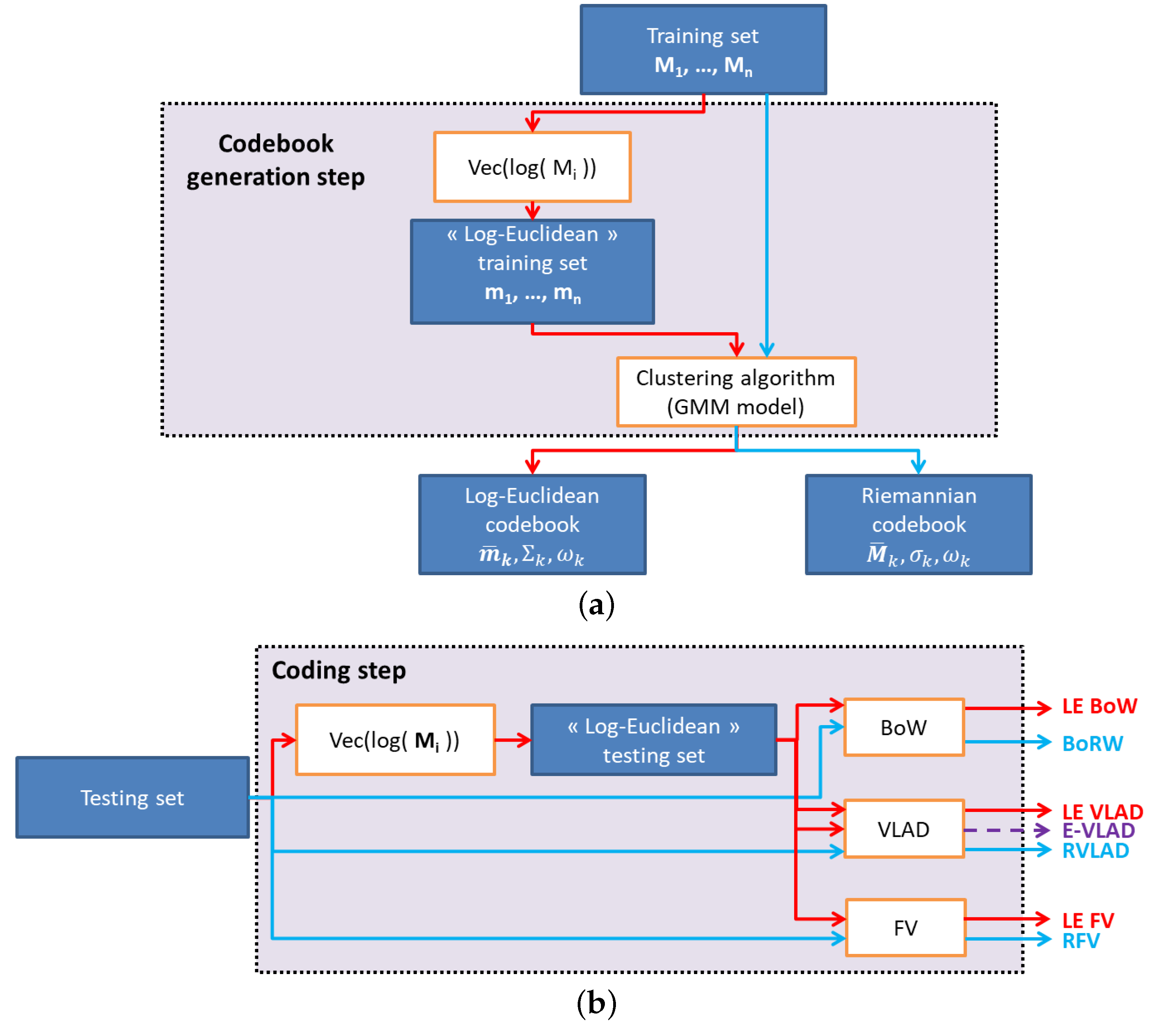
Figure 2 draws an overview of the relation between the different approaches based on the BoW, VLAD and FV models. The LE-based metric approaches appear in red while the affine invariant ones are displayed in blue. The E-VLAD descriptor is displayed in purple since it considers the Riemannian codebook combined with LE representation of the features.

4.1. Bag of Words Descriptor

One of the most common encoding methods is represented by the BoW model. With this model, a set of features is encoded in an histogram descriptor obtained by counting the number of features which are closest to each codeword of the codebook. In the beginning, this descriptor has been employed for text retrieval and categorization [10,55], by modeling a text with an histogram containing the number of occurrences of each word. Later on, the BoW model has been extended to visual categorization [56], where images are described by a set of descriptors, such as SIFT features. In such case, the “words” of the codebook are obtained by considering a clustering algorithm with the standard Euclidean metric. Recently, the BoW model has been extended to features lying in a non-Euclidean space, such as SPD matrices. In this context, two approaches have been proposed based respectively on the LE and affine invariant Riemannian metrics:
  • the log-Euclidean bag of words (LE BoW) [33,35].
  • the bag of Riemannian words (BoRW) [36].
These two descriptors have been employed successfully for different applications, including texture and human epithelial type 2 cells classification [36], action recognition [33,35].

4.1.1. Log-Euclidean Bag of Words (LE BoW)

The LE BoW model has been considered in [33,35]. First, the space of covariance matrices is embedded into a vector space by considering the LE vector representation m given in (1). With this embedding, the LE BoW model can be interpreted as the BoW model in the LE space. This means that codewords are elements of the log-Euclidean codebook detailed in Section 3.1. Next, each observed SPD matrix M n is assigned to cluster k of closest codeword m ¯ k to compute the histogram descriptor. The vicinity is evaluated here as the Euclidean distance between the LE vector representation m n and the codeword m ¯ k .
The LE BoW descriptor can also be interpreted by considering the Gaussian mixture model recalled in (2). In such case, each feature m n is assigned to the cluster k, for k = 1 , , K according to:
arg max k ϖ k p ( m n | m ¯ k , Σ k ) ,
where p ( m n | m ¯ k , Σ k ) is the multivariate Gaussian distribution given in (3). In addition, two constraints are assumed k = 1 , , K :
  • the homoscedasticity assumption:
    Σ k = Σ .
  • the same weight is given to all mixture components:
    ϖ k = 1 K .

4.1.2. Bag of Riemannian Words (BoRW)

This descriptor has been introduced in [36]. Contrary to the LE BoW model, the BoRW model exploits the affine invariant Riemannian metric. For that, it considers the Riemannian codebook detailed in Section 3.2. Then, the histogram descriptor is computed by assigning each SPD matrix to the cluster k of the closest codebook element M ¯ k , the proximity being measured with the geodesic distance recalled in (8).
As for the LE BoW descriptor, the definition of the BoRW descriptor can be obtained by the Gaussian mixture model, except that the RGD model defined in (12) is considered instead of the multivariate Gaussian distribution. Each feature M n is assigned to the cluster k, for k = 1 , , K according to:
arg max k ϖ k p ( M n | M ¯ k , σ k ) .
In addition, the two previously cited assumptions are made, that are the same dispersion and weight are given to all mixture components.
It has been shown in the literature that the performance of BoW descriptors depends on the codebook size, best results being generally obtained for large dictionaries [5]. Moreover, BoW descriptors are based only on the number of occurrences of each codeword from the dataset. In order to increase the classification performances, second order statistics can be considered. This is the case of VLAD and FV that are presented next.

4.2. Vectors of Locally Aggregated Descriptors

VLAD descriptors have been introduced in [2] and represent a method of encoding the difference between the codewords and the features. For features lying in a Euclidean space, the codebook is composed by cluster centroids { ( x ¯ k ) 1 k K } obtained by clustering algorithm on the training set. Next, to encode a feature set { ( x n ) 1 n N } , vectors v k containing the sum of differences between codeword and feature samples assigned to it are computed for each cluster:
v k = x n c k x n x ¯ k .
The final VLAD descriptor is obtained as the concatenation of all vectors v k :
VLAD = [ v 1 T , , v K T ] .
To generalize this formalism to features lying in a Riemannian manifold, two theoretical aspects should be addressed carefully, which are the definition of a metric to describe how features are assigned to the codewords, and the definition of subtraction operator for these kind of features. By addressing these aspects, three approaches have been proposed in the literature:
  • the log-Euclidean vector of locally aggregated descriptors (LE VLAD) [11].
  • the extrinsic vector of locally aggregated descriptors (E-VLAD) [37].
  • the intrinsic Riemannian vector of locally aggregated descriptors (RVLAD) [11].

4.2.1. Log-Euclidean Vector of Locally Aggregated Descriptors (LE VLAD)

This descriptor has been introduced in [11] to encode a set of SPD matrices with VLAD descriptors. In this approach, VLAD descriptors are computed in the LE space. For this purpose, (24) is rewritten as:
v k = m n c k m n m ¯ k ,
where the LE representation m n of M n belongs to the cluster c k if it is closer to m ¯ k than any other element of the LE codebook. The proximity is measured here according to the Euclidean distance between the LE vectors.

4.2.2. Extrinsic Vector of Locally Aggregated Descriptors (E-VLAD)

The E-VLAD descriptor is based on the LE vector representation of SPD matrices. However, contrary to the LE VLAD model, this descriptor uses the Riemannian codebook to define the Voronoï regions. It yields that:
v k = M n c k m n m ¯ k ,
where M n belongs to the cluster c k if it is closer to M ¯ k according to the affine invariant Riemannian metric. Note also that here m ¯ k is the LE vector representation of the Riemannian codebook element M ¯ k .
To speed-up the processing time, Faraki et al. have proposed in [37] to replace the affine invariant Riemannian metric by the Stein metric [57]. For this latter, computational cost to estimate the centroid of a set of covariance matrices is less demanding than with the affine invariant Riemannian metric since a recursive computation of the Stein center from a set of covariance matrices has been proposed in [58].
Since this approach exploits two metrics, one for the codebook creation (with the affine invariant Riemannian or Stein metric) and another for the coding step (with the LE metric), we referred it as an extrinsic method.

4.2.3. Riemannian Vector of Locally Aggregated Descriptors (RVLAD)

This descriptor has been introduced in [11] to propose a solution for the affine invariant Riemannian metric. More precisely, the geodesic distance [47] recalled in (8) is considered to measure similarity between SPD matrices. The affine invariant Riemannian metric is used to define the Voronoï regions) and the Riemannian logarithm mapping [48] is used to perform the subtraction on the manifold. It yields that for the RVLAD model, the vectors v k are obtained as:
v k = Vec M n c k Log M ¯ k ( M n ) ,
where Log M ¯ k ( · ) is the Riemannian logarithm mapping defined in (11). Please note that the vectorization operator Vec ( · ) is used to represent v k as a vector.
As explained in [2], the VLAD descriptor can be interpreted as a simplified non probabilistic version of the FV. In the next section, we give an explicit relationship between these two descriptors which is one of the main contribution of the paper.

4.3. Fisher Vector Descriptor

Fisher vectors (FV) are descriptors based on Fisher kernels [59]. FV measures how samples are correctly fitted by a given generative model p ( X | θ ) . Let X = { X n } n = 1 : N , be a sample of N observations. The FV descriptor associated to X is the gradient of the sample log-likelihood with respect to the parameters θ of the generative model distribution, scaled by the inverse square root of the Fisher information matrix (FIM).
First, the gradient of the log-likelihood with respect to the model parameter vector θ , also known as the Fisher score (FS) U X [59], should be computed:
U X = θ log p ( X | θ ) = θ n = 1 N log p ( X n | θ ) .
As mentioned in [5], the gradient describes the direction in which parameters should be modified to best fit the data. In other words, the gradient of the log-likelihood with respect to a parameter describes the contribution of that parameter to the generation of a particular feature [59]. A large value of this derivative is equivalent to a large deviation from the model, suggesting that the model does not correctly fit the data.
Second, the gradient of the log-likelihood can be normalized by using the FIM I θ [59]:
I θ = E X [ U X U X T ] ,
where E X [ · ] denotes the expectation over p ( X | θ ) . It yields that the FV representation of X is given by the normalized gradient vector [5]:
G θ X = I θ 1 / 2 θ log p ( X | θ ) .
As reported in previous works, exploiting the FIM I θ in the derivation of FV yields to excellent results with linear classifiers [6,7,9]. However, the computation of the FIM might be quite difficult. It does not admit a close-form expression for many generative models. In such case, it can be approximated empirically by carrying out a Monte Carlo integration, but this latter can be costly especially for high dimensional data. To solve this issue, some analytical approximations can be considered [5,9].
The next part explains how the FV model can be used to encode a set of SPD matrices. Once again, two approaches are considered by using respectively the LE and the affine invariant Riemannian metrics:
  • the Log-Euclidean Fisher vectors (LE FV).
  • the Riemannian Fisher vectors (RFV) [40].

4.3.1. Log-Euclidean Fisher Vectors (LE FV)

The LE FV model consists in an approach where the FV descriptors are computed in the LE space. In such case, the multivariate Gaussian mixture model recalled in (2) is considered.
Let M L E = { m n } n = 1 : N be the LE representation of the set M . To compute the LE FV descriptor of M , the derivatives of the log-likelihood function with respect to θ should first be computed. Let γ k ( m n ) be the soft assignment of m n to the kth Gaussian component
γ k ( m n ) = ϖ k p ( m n | θ k ) j = 1 K ϖ j p ( m n | θ j ) .
It yields that, the elements of the LE Fisher score (LE FS) are obtained as:
log p ( M L E | θ ) m ¯ k d = n = 1 N γ k ( m n ) m n d m ¯ k d σ k d 2 ,
log p ( M L E | θ ) σ k d = n = 1 N γ k ( m n ) m n d m ¯ k d 2 σ k d 3 1 σ k d ,
log p ( M L E | θ ) α k = n = 1 N γ k ( m n ) ϖ k ,
where m ¯ k d (resp. σ k d ) is the dth element of vector m ¯ k (resp. σ k ). Please note that to ensure the constraints of positivity and sum-to-one for the weights ϖ k , the derivative of the log-likelihood with respect to this parameter is computed by taking into consideration the soft-max parametrization as proposed in [9,60]:
ϖ k = exp ( α k ) j = 1 K exp ( α j ) .
Under the assumption of nearly hard assignment, that is the soft assignment distribution γ k ( m n ) is sharply peaked on a single value of k for any observation m n , the FIM I θ is diagonal and admits a close-form expression [9]. It yields that the LE FV of M is obtained as:
G m ¯ k d M L E = 1 ϖ k n = 1 N γ k ( m n ) m n d m ¯ k d σ k d ,
G σ k d M L E = 1 2 ϖ k n = 1 N γ k ( m n ) m n d m ¯ k d 2 σ k d 2 1 ,
G α k M L E = 1 ϖ k n = 1 N γ k ( m n ) ϖ k .

4.3.2. Riemannian Fisher Vectors (RFV)

Ilea et al. have proposed in [40] an approach to encode a set of SPD matrices with FS based on the affine invariant Riemannian metric: the Riemannian Fisher score (RFS). In this method, the generative model is a mixture of RGDs [39] as presented in Section 3.2.2. By following the same procedure as before, the RFS is obtained by computing the derivatives of the log-likelihood function with respect to the distribution parameters θ = { ( ϖ k , M ¯ k , σ k ) 1 k K } . It yields that [40]:
log p ( M | θ ) M ¯ k = n = 1 N γ k ( M n ) Log M ¯ k ( M n ) σ k 2 ,
log p ( M | θ ) σ k = n = 1 N γ k ( M n ) d 2 ( M n , M ¯ k ) σ k 3 Z ( σ k ) Z ( σ k ) ,
log p ( M | θ ) α k = n = 1 N γ k ( M n ) ϖ k ,
where Log M ¯ k ( · ) is the Riemannian logarithm mapping in (11) and Z ( σ k ) is the derivative of Z ( σ k ) with respect to σ k . The function Z ( σ ) can be computed numerically by a Monte Carlo integration, in a similar way to the one for the normalization factor Z ( σ ) (see Section 3.2.2).
In these expressions, γ k ( M n ) represents the probability that the feature M n is generated by the kth mixture component, computed as:
γ k ( M n ) = ϖ k p ( M n | M ¯ k , σ k ) j = 1 K ϖ j p ( M n | M ¯ j , σ j ) .
By comparing (33)–(35) with (40)–(42), one can directly notice the similarity between the LE FS and the RFS. In these equations, vector difference in the LE FS is replaced by log map function in the RFS. Similarly, Euclidean distance in the LE FS is replaced by geodesic distance in the RFS.
In [40], Ilea et al. have not exploited the FIM. In this paper, we propose to add this term in order to define the Riemannian Fisher vectors (RFV). To derive the FIM, the same assumption as the one given in Section 4.3.1 should be made, i.e., the assumption of nearly hard assignment, that is the soft assignment distribution γ k ( M n ) is sharply peaked on a single value of k for any observation M n . In that case, the FIM is block diagonal and admits a close-form expression detailed in [61]. In this paper, Zanini et al. have used the FIM to propose an online algorithm for estimating the parameters of a Riemannian Gaussian mixture model. Here, we propose to add this matrix in another context which is the derivation of a descriptor: the Riemannian FV.
First, let’s recall some elements regarding the derivation of the FIM. This block diagonal matrix is composed of three terms, one for the weight, one for the centroid and one for the dispersion.
  • For the weight term, the same procedure as the one used in the conventional Euclidean framework can employed [9]. In [61], they proposed another way to derive this term by using the notation s = ϖ 1 , , ϖ K and observing that s belongs to a Riemannian manifold (more precisely the ( K 1 ) -sphere S K 1 ). These two approaches yield exactly to the same final result.
  • For the centroid term, it should be noted that each centroid M ¯ k is a covariance matrix which lives in the manifold P m of m × m symmetric positive definite matrices. To derive the FIM associated to this term, the space P m should be decomposed as the product of two irreducible manifolds, i.e., P m = R × SP m where SP m is the manifold of symmetric positive definite matrices with unitary determinant. Hence, each observed covariance matrix M can be decomposed as ϕ ( M ) = M 1 , M 2 where
    -
    M 1 = log det M is a scalar element lying in R .
    -
    M 2 = e M 1 m M is a covariance matrix of unit determinant.
  • For the dispersion parameter, the notation η = 1 2 σ 2 is considered to ease the mathematical derivation. Since this parameter is real, the conventional Euclidean framework is employed to derive the FIM. The only difference is that the Euclidean distance is replaced by the geodesic one.
For more information on the derivation of the FIM for the Riemannian Gaussian mixture model, the interested reader is referred to [61]. To summarize, the elements of the block-diagonal FIM for the Riemannian Gaussian mixture model are defined by:
I s = 4 I K ,
I M ¯ k 1 = ϖ k σ k 3 ,
I M ¯ k 2 = ϖ k ψ 2 ( η k ) σ k 4 m ( m + 1 ) 2 1 I m ( m + 1 ) 2 1 ,
I η k = ϖ k ψ ( η k ) ,
where I K is the K × K identity matrix, ψ ( η ) = log Z ( σ ) and ψ ( · ) (resp. ψ ( · ) ) are the first (resp. the second) order derivatives of the ψ ( · ) function with respect to η . ψ 2 ( η ) = ψ ( η ) + 1 2 η .
Now that the FIM and the FS score are obtained for the Riemannian Gaussian mixture model, we can define the RFV by combining (40) to (42) and (44) to (47) in (31). It yields that:
G M ¯ k 1 M = 1 ϖ k n = 1 N γ k ( M n ) M ¯ k 1 M n 1 σ k ,
G M ¯ k 2 M = 1 ϖ k n = 1 N γ k ( M n ) m ( m + 1 ) 2 1 ψ 2 η k Log M ¯ k 2 ( M n ) 2 ,
G σ k M = 1 ϖ k n = 1 N γ k ( M n ) d 2 ( M n , M ¯ k ) ψ ( η k ) ψ ( η k ) ,
G ϖ k M = 1 ϖ k n = 1 N γ k ( M n ) ϖ k .
Unsurprisingly, this definition of the RFV can be interpreted as a direct extension of the FV computed in the Euclidean case to the Riemannian case. In particular (37)–(39) are retrieved when the normalization factor Z ( σ ) is set to σ 2 π in (48), (50) and (51).
In the end, the RFVs are obtained by concatenating some, or all of the derivatives in (48)–(51). Note also that since (49) is a matrix, the vectorization operator Vec ( · ) is used to represent it as a vector.

4.3.3. Relation with VLAD

As stated before, the VLAD descriptor can be retrieved from the FV model. In this case, only the derivatives with respect to the central element ( m ¯ k d or M ¯ k ) are considered. Two assumptions are also made:
  • the hard assignment scheme, that is:
    γ k ( M ) = 1 , if M c k 0 , otherwise ,
    where M c k are the elements assigned to cluster c k and k = 1 , , K ,
  • the homoscedasticity assumption, that is σ k = σ , k = 1 , , K .
By taking into account these hypotheses, it can be noticed that (33) reduces to (26), confirming that LE FV are a generalization of LE VLAD descriptors. The same remark can be done for the approach exploiting the affine invariant Riemannian metric where the RFV model can be viewed as an extension of the RVLAD model. The proposed RFV gives a mathematical explanation of the RVLAD descriptor which has been introduced in [11] by an analogy between the Euclidean space (for the VLAD descriptor) and the Riemannian manifold (for the RVLAD descriptor).

4.4. Post-Processing

Once the set of SPD matrices is encoded by one of the previously exposed coding methods (BoW, VLAD, FS or FV), a post-processing step is classically employed. In the framework of feature coding, the post-processing step consists in two possible normalization steps: the power and 2 normalization. These operations are detailed next.

4.4.1. Power Normalization

The purpose of this normalization method is to correct the independence assumption that is usually made on the image patches [7]. For the same vector v , its power-normalized version v p o w e r is obtained as:
v p o w e r = sign ( v ) | v | ρ ,
where 0 < ρ 1 , and sign ( · ) is the signum function and | · | is the absolute value. In practice, ρ is set to 1 2 , as suggested in [9].

4.4.2. 2 Normalization

This normalization method has been proposed in [6] to minimize the influence of the background information on the image signature. For a vector v , its normalized version v L 2 is computed as:
v L 2 = v v 2 ,
where · 2 is the L 2 norm.
Depending on the considered coding method, one or both normalization steps are applied. For instance, for VLAD, FS and FV-based methods, both normalizations are used [36,40], while for BoW based methods only the 2 normalization is considered [33].

4.5. Synthesis

Table 1 draws an overview of the different coding methods. As seen before, two metrics can be considered, namely the LE and the affine invariant Riemannian metrics. This yields to two Gaussian mixture models: a mixture of multivariate Gaussian distributions and a mixture of Riemannian Gaussian distributions. These mixture models are the central point in the computation of the codebook which are further used to encode the features. In this table and in the following ones, the proposed coding methods are displayed in gray.
As observed, a direct parallel can be drawn between the different coding methods (BoW, VLAD, FS and FV). More precisely, it is interesting to note how the conventional coding methods used for descriptors lying in R m ( m + 1 ) 2 are adapted to covariance matrix descriptors.

5. Application to Image Classification

This section introduces some applications to image classification. Two experiments are conducted, one for texture image classification and one for head pose image classification. The aim of these experiments is three-fold. The first objective is to compare two Riemannian metrics: the log-Euclidean and the affine invariant Riemmannian metrics. The second objective is to analyze the potential of the proposed FV-based methods compared to the recently proposed BoW and VLAD-based models. In addition, finally, the third objective is to evaluate the advantage of including the FIM in the derivation of the FVs, i.e., comparing the performance between FS and FV.

5.1. Texture Image Classification

5.1.1. Image Databases

To answer these questions, a first experiment is conducted on four conventional texture databases, namely the VisTex [62], Brodatz [63], Outex-TC-00013 [64] and USPtex [65] databases. Some examples of texture images issued from these four texture databases are displayed in Figure 3.
The VisTex database is composed of 40 texture images of size 512 × 512 pixels. In the following, each texture image is divided into 64 non-overlapping images of size 64 × 64 pixels, yielding to a database of 2560 images. The grayscale Brodatz database contains 112 textures images of size 640 × 640 pixels which represent a large variety of natural textures. Each one is divided into 25 non-overlapping images of size 128 × 128 pixels, thus creating 2800 images in total (i.e., 112 classes with 25 images/class). The Outex database consists of a dataset of 68 texture classes (canvas, stone, wood, …) with 20 image samples per class of size 128 × 128 pixels. In addition, finally, The USPtex database is composed of 191 texture classes with 12 image samples of size 128 × 128 pixels. Table 2 summarizes the main characteristics of each of these four databases.

5.1.2. Context

As shown in Figure 1, the first stage is the feature extraction step which consists in representing each texture image by a set of covariance matrices. Since the experiment purpose is not to find the best classification accuracies on these databases, but rather to compare the different strategies (choice of the metric, influence of the coding model) on the same features, we have adopted the simple but effective region covariance descriptors (RcovD) used in [34]. The extracted RCovD are the estimated covariance matrices of vectors v ( x , y ) computed on sliding patches of size 15 × 15 pixels where:
v ( x , y ) = I ( x , y ) , I ( x , y ) x , I ( x , y ) y , 2 I ( x , y ) x 2 , 2 I ( x , y ) y 2 T .
In this experiment, the patches are overlapped by 50 % . The fast covariance matrix computation algorithm based on integral images presented in [34] is adopted to speed-up the computation time of this feature extraction step. It yields that each texture class is composed by a set M 1 , , M N of N covariance matrices, that are elements in P 5 .
For each class, codewords are represented by the estimated parameters of the mixture of K Gaussian distributions. For this experiment, the number of modes K is set to 3. In the end, the codebook is obtained by concatenating the previously extracted codewords (for each texture class). Please note that the same number of modes K has been considered for each class and has been set experimentally to 3 which represents a good trade-off between the model complexity and the within-class diversity. This parameter has been fixed for all these experiments since the aim is to fairly compare the different coding strategies for the same codebook.
Once the codebook is created, the covariance matrices of each image are encoded by one of the previously described method (namely BoW, VLAD, FS or FV) adapted to the LE or affine invariant Riemannian metric. Then after some post-processing (power and/or 2 normalization), the obtained feature vectors are classified. Here, the SVM classifier with Gaussian kernel is used. The parameter of the Gaussian kernel is optimized by using a cross validation procedure on the training set.
The whole procedure is repeated 10 times for different training and testing sets. Each time, half of the database is used for training while the remaining half is used for testing. Table 3, Table 4, Table 5 and Table 6 show the classification performance in term of overall accuracy (mean ± standard deviation) on the VisTex, Brodatz, Outex and USPtex databases. In these tables, the best classification results are displayed.
As the FS and FV descriptors are obtained by deriving the log-likelihood function with respect to the weight, dispersion and centroid parameters, the contribution of each term to the classification accuracy can be analyzed. Therefore, different versions of the FS and FV descriptors can be considered to analyze separately the contribution of each term or by combining these different terms. For example, the row “LE FS/RFS: M ¯ ” indicates the classification results when only the derivatives with respect to the centroid are considered to derive the FS (see (33) and (40)). In the following, only the results employing the mean are presented since the state-of-the-art have already proved that the mean provides the most significant information [6,7].
Please note that the use of the FIM in the derivation of the FV allows to improve the classification accuracy. As observed for the four considered databases, a gain of about 1 % to 3 % is obtained when comparing “LE FV/RFV: M ¯ ” with “LE FS/RFS: M ¯ ”.
For these four experiments on texture image classification, the proposed FV descriptors outperform the state-of-the-art BoW and VLAD-based descriptors. Classifying with the best FV descriptor yields to a gain of about 1 % to 4 % compared to the best BoW and VLAD-based descriptors.

5.1.3. Comparison between Anisotropic and Isotropic Models

As observed in Table 3, Table 4, Table 5 and Table 6, the performance for the LE metric are generally better than that with the affine invariant Riemannian metric. However, both approaches are not directly comparable since an anisotropic model is considered for the LE metric while an isotropic model is used for the affine invariant Riemannian metric. Indeed, for the former the dispersion for the Gaussian mixture model is a diagonal matrix Σ k while for the latter the dispersion σ k is a scalar. To provide a fairer comparison between these two approaches, an experiment is conducted to illustrate if the observed gain with the LE metric comes from the metric or from the fact that the Gaussian model is anisotropic.
For the LE metric, an isotropic model can be built by considering that Σ k = σ k 2 I m ( m + 1 ) 2 . For the affine invariant Riemannian metric, the Riemannian Gaussian distribution recalled in Section 3.2.2 is isotropic. Pennec has introduced in [66] an anisotropic Gaussian model, but for this latter the normalization factor depends on both the centroid M k ¯ and the concentration matrix. It yields that the computation of the FS score and the derivation of the FIM for this model are still an open problem. This model will not be considered in the following.
Table 7 shows the classification results obtained on the four considered texture databases. Here, the performances are displayed for the FV descriptor computed by using the derivative with respect to the centroid (i.e., LE FV/RFV: M ¯ ). It can be noticed that for the LE metric, an anisotropic model yields to a significant gain of about 4 % to 7 % compared to an isotropic model. More interestingly, for an istropic model, descriptors based on the affine invariant Riemannian metric yield to better performances than that obtained with the LE metric. A gain of about 2 % to 6 % is observed. These experiments clearly illustrate that the gain observed in Table 3, Table 4, Table 5 and Table 6 for the LE metric comes better from the anistropicty of the Gaussian mixture model than from the metric definition. According to these observations, it is expected that classifying with FV issued from anistropic Riemannian Gaussian mixture model will improve the performance. This point will be subject of future research works including the derivation of normalization factor of the anistropic Riemannian Gaussian model and the computation of the FIM.

5.2. Head Pose Classification

5.2.1. Context

The aim of this second experiment is to illustrate how the proposed framework can be used for classifying a set of covariance matrices of larger dimension. Here, the head pose classification problem is investigated on the HOCoffee dataset [67]. This dataset contains 18,117 head images of size 50 × 50 pixels with six head pose classes (front left, front, front right, left, rear and right). Some examples of images of each class (one class per row) are displayed in Figure 4. It has a predefined experiment protocol where 9522 images are used for training and the remaining 8595 images are used for testing. We follow the same experiment protocol as in [11]. The extracted RCovD are the estimated covariance matrices of vectors v ( x , y ) computed on sliding patches of size 15 × 15 pixels where:
v ( x , y ) = I L ( x , y ) , I a ( x , y ) , I b ( x , y ) , I x 2 ( x , y ) + I y 2 ( x , y ) , arctan I x ( x , y ) I y ( x , y ) , G 1 ( x , y ) , , G 8 ( x , y ) T
with I c ( x , y ) , c { L , a , b } are the CIELab color information for the pixel at coordinate ( x , y ) , I x ( x , y ) and I y ( x , y ) are the first order luminance derivatives, and G i ( x , y ) denotes the response of the i-th Difference Of Offset Gaussian (DOOG) filter-bank centered at position ( x , y ) of I L . An overlap of 50 % is considered to compute the covariance matrices. Hence, each image in the database is represented by a set of 25 covariance matrices of size 13 × 13 . As for the previous experiment, 3 atoms per class are considered to compute the codebook.
Table 8 shows the classification accuracy on the HOCoffee dataset. Similar conclusions can be drawn with the previous experiment on texture image classification. The use of the FIM in the derivation of the FV still allows to improve the classification accuracy. The best performances are obtained for the LE metric compared to the affine invariant Riemannian metric. Nevertheless, for this latter, the performance are quite low, especially for the FV obtained by deriving with respect to the dispersion parameter. Please note that for this experiment the RVLAD descriptor allows to obtain better classification accuracy than the best RFV ( 70.6 % vs. 67.9 % ).
To understand why the performance with RFV are relatively low for the HOCoffee dataset, an experiment is conducted to see if the dispersion parameter can be considered with confidence.

5.2.2. Estimation Performance

This section presents simulation results to evaluate the performance of the estimator of the dispersion parameter for Gaussian models based on the LE and affine invariant Riemannian metrics. For all these experiments,
M ¯ i j = ρ | i j | for i , j 0 , m 1 .
ρ is set to 0.7 in the following. For the LE metric, N i.i.d. vector samples ( x 1 , , x N ) are generated according to a multivariate Gaussian distribution N ( m ¯ , Σ ) , with Σ = σ 2 I m ( m + 1 ) 2 . For the affine invariant Riemannian metric, N i.i.d. covariance matrix samples are generated according the Riemannian Gaussian distribution defined in Section 3.2.2. In the following, 1000 Monte Carlo runs have been used to evaluate the performance of the estimation algorithm.
Figure 5 draws the evolution of the root mean square error (RMSE) of the dispersion parameter σ for Gaussian models based on the LE and affine invariant Riemannian metrics as a function of σ . The red curve corresponds to an experiment with covariance matrices of dimension 5 × 5 , while the blue one is for 13 × 13 covariance matrices. In this figure, 1000 (resp. 10,000) covariance matrices samples issued from the Gaussian model are generated to plot the solid (resp. the dashed) curve. This yields that the texture classification experiment of Section 5 is mimicked with the solid red curve while the head pose classification experiment is mimicked with the dashed blue one. As observed in Figure 5a for the LE m etric, the RMSE of the dispersion parameter is mainly influenced by the number of generated samples N. For this LE metric, the dimension of the covariance matrices has less importance, since the red and blue curves are superposed. Nevertheless, for the affine invariant Riemannian metric in Figure 5b, the RMSE of the dispersion parameter is greatly influenced by the dimension of the covariance matrices, especially for large values of σ .
For the five databases, Figure 6 shows the boxplots of the dispersion parameter for the LE (Figure 6a) and Riemannian (Figure 6b) codebooks. Please note that since two different metrics are considered, the amplitude value of the dispersion parameter are not directly comparable between Figure 6a,b. However, for a given metric, it is possible to analyze the variability of the dispersion parameter for the five experiments. As observed in Figure 6b, the estimated dispersion parameter σ k for the Riemannian codebook takes larger values for the HOCoffee dataset than that for the four texture datasets. For the former, the estimated dispersion parameters of the Riemannian codebook are larger than 0.4 which corresponds to the area in Figure 5b where the RMSE of σ increases greatly. This explains why the performance with the RFV (especially when the dispersion is considered) are relatively low compared to the LE FV. Indeed, as observed in Figure 5a for the LE codebook, the dispersion parameters are much more comparable for the five datasets and the dimension m of the observed covariance matrix has less impact on the RMSE of σ for the LE metric.

5.3. Computation Time

The computation time can be separated in two parts:
  • The first one concerns the time used in learning stage to generate the codebook.
  • The second one concerns the time used to encode an image.
Obviously the codebook generation step requires much more time than the coding step. However, this codebook generation step can be done offline. This is similar to a deep learning approach where the estimation of the model takes much more time than the classification itself. Table 9 summarizes these computation times for the experiment on the VisTex database. For the coding method, the LE FV and RFV descriptors with only the derivative with respect to the centroid m ¯ or M ¯ are considered. All the implementations are carried out using MATLAB 2017 on a PC machine Core i7-4790 3.6GHz, 16GB RAM.
As expected, the LE metric allows to faster the computation time compared to the affine invariant Riemannian metric. A gain of a factor of 6 is observed for the coding time with the log-Euclidean metric for 5 × 5 covariance matrices.

6. Conclusions

Starting from the Gaussian mixture model (for the LE metric) and the Riemannian Gaussian mixture model (for the affine invariant Riemannian metric), we have proposed a unified view of coding methods. The proposed LE FV and RFV can be interpreted as a generalization of the BoW and VLAD-based approaches. The experimental results have shown that: (i) the use of the FIM in the derivation of the FV allows to improve the classification accuracy, (ii) the proposed FV descriptors outperform the state-of-the-art BoW and VLAD-based descriptors, and (iii) the descriptors based on the LE metric lead to better classification results than those based on the affine invariant Riemannian metric. For this latter observation, the gain observed with the LE metric comes better from the anistropicty of the Gaussian mixture model than on the metric itself. For isotropic models, FV described issued from the affine invariant Riemannian metric leads to better results than those obtained with the LE metric. It is hence expected that the definition of a FV issued from an anistropic Riemannian Gaussian mixture model will improve the performance. This point represents one of the main perspective of this research work.
For larger covariance matrices, the last experiment on head pose classification has illustrated the limits of the RFV issued from the Riemannian Gaussian mixture model. It has been shown that the root mean square error of the dispersion parameter σ can be large for high value of σ ( σ > 0.4 ). In that case, the LE FV are a good alternative to the RFV.
Future works will include the use of the proposed FV coding for covariance matrices descriptors in a hybrid classification architecture which will combine them with convolutional neural networks [17,18,19].

Author Contributions

All the authors contributed equally for the mathematical development and the specification of the algorithms. I.I. and L.B. conducted the experiments and wrote the paper. Y.B. gave the central idea of the paper and managed the main tasks and experiments. All the authors read and approved the final manuscript.

Funding

This research received no external funding.

Conflicts of Interest

The authors declare no conflict of interest.

References

  1. Sivic, J.; Russell, B.C.; Efros, A.A.; Zisserman, A.; Freeman, W.T. Discovering objects and their location in images. In Proceedings of the Tenth IEEE International Conference on Computer Vision (ICCV ’05), Beijing, China, 17–21 October 2005; Volume 1, pp. 370–377. [Google Scholar] [CrossRef]
  2. Jégou, H.; Douze, M.; Schmid, C.; Pérez, P. Aggregating local descriptors into a compact image representation. In Proceedings of the IEEE Conference on Computer Vision and Pattern Recognition, San Francisco, CA, USA, 13–18 June 2010. [Google Scholar]
  3. Arandjelović, R.; Zisserman, A. All about VLAD. In Proceedings of the IEEE Conference on Computer Vision and Pattern Recognition, Portland, OR, USA, 23–28 June 2013. [Google Scholar]
  4. Tsuda, K.; Kawanabe, M.; Müller, K.R. Clustering with the Fisher Score. In Proceedings of the 15th International Conference on Neural Information Processing Systems, NIPS ’02, Vancouver, BC, Canada, 9–14 December 2002; MIT Press: Cambridge, MA, USA, 2002; pp. 745–752. [Google Scholar]
  5. Perronnin, F.; Dance, C. Fisher kernels on visual vocabularies for image categorization. In Proceedings of the IEEE Conference on Computer Vision and Pattern Recognition, Minneapolis, MN, USA, 17–22 June 2007; pp. 1–8. [Google Scholar]
  6. Perronnin, F.; Sánchez, J.; Mensink, T. Improving the Fisher kernel for large-scale image classification. In Computer Vision—ECCV 2010; Daniilidis, K., Maragos, P., Paragios, N., Eds.; Lecture Notes in Computer Science; Springer: Berlin/Heidelberg, Germnay, 2010; Volume 6314, pp. 143–156. [Google Scholar] [CrossRef]
  7. Perronnin, F.; Liu, Y.; Sánchez, J.; Poirier, H. Large-scale image retrieval with compressed Fisher vectors. In Proceedings of the Twenty-Third IEEE Conference on Computer Vision and Pattern Recognition, San Francisco, CA, USA, 13–18 June 2010; pp. 3384–3391. [Google Scholar] [CrossRef]
  8. Douze, M.; Ramisa, A.; Schmid, C. Combining attributes and Fisher vectors for efficient image retrieval. In Proceedings of the IEEE Conference on Computer Vision and Pattern Recognition, Colorado Springs, CO, USA, 20–25 June 2011; pp. 745–752. [Google Scholar] [CrossRef]
  9. Sánchez, J.; Perronnin, F.; Mensink, T.; Verbeek, J. Image classification with the Fisher vector: Theory and practice. Int. J. Comput. Vis. 2013, 105, 222–245. [Google Scholar] [CrossRef]
  10. Salton, G.; Buckley, C. Term-weighting approaches in automatic text retrieval. Inf. Process. Manag. 1988, 24, 513–523. [Google Scholar] [CrossRef] [Green Version]
  11. Faraki, M.; Harandi, M.T.; Porikli, F. More about VLAD: A leap from Euclidean to Riemannian manifolds. In Proceedings of the IEEE Conference on Computer Vision and Pattern Recognition, Boston, MA, USA, 7–12 June 2015; pp. 4951–4960. [Google Scholar] [CrossRef]
  12. Le Cun, Y.; Boser, B.E.; Denker, J.S.; Henderson, D.; Howard, R.E.; Hubbard, W.E.; Jackel, L.D. Handwritten Digit Recognition with a Back-Propagation Network. In Advances in Neural Information Processing Systems 2; Touretzky, D.S., Ed.; Morgan-Kaufmann: San Francisco, CA, USA, 1990; pp. 396–404. [Google Scholar]
  13. Krizhevsky, A.; Sutskever, I.; Hinton, G.E. ImageNet Classification with Deep Convolutional Neural Networks. In Proceedings of the 25th International Conference on Neural Information Processing Systems, NIPS ’12, Lake Tahoe, NV, USA, 3–6 December 2012; Volume 1, pp. 1097–1105. [Google Scholar]
  14. Chandrasekhar, V.; Lin, J.; Morère, O.; Goh, H.; Veillard, A. A Practical Guide to CNNs and Fisher Vectors for Image Instance Retrieval. Signal Process. 2016, 128, 426–439. [Google Scholar] [CrossRef]
  15. Perronnin, F.; Larlus, D. Fisher vectors meet Neural Networks: A hybrid classification architecture. In Proceedings of the 2015 IEEE Conference on Computer Vision and Pattern Recognition (CVPR), Boston, MA, USA, 7–12 June 2015; pp. 3743–3752. [Google Scholar] [CrossRef]
  16. Simonyan, K.; Vedaldi, A.; Zisserman, A. Deep Fisher Networks for Large-scale Image Classification. In Proceedings of the 26th International Conference on Neural Information Processing Systems, NIPS ’13, Lake Tahoe, NV, USA, 5–10 December 2013; Volume 1, pp. 163–171. [Google Scholar]
  17. Ng, J.Y.; Yang, F.; Davis, L.S. Exploiting Local Features from Deep Networks for Image Retrieval. arXiv, 2015; arXiv:1504.05133. [Google Scholar]
  18. Cimpoi, M.; Maji, S.; Kokkinos, I.; Vedaldi, A. Deep Filter Banks for Texture Recognition, Description, and Segmentation. Int. J. Comput. Vis. 2016, 118, 65–94. [Google Scholar] [CrossRef] [PubMed] [Green Version]
  19. Diba, A.; Pazandeh, A.M.; Gool, L.V. Deep visual words: Improved fisher vector for image classification. In Proceedings of the 2017 Fifteenth IAPR International Conference on Machine Vision Applications (MVA), Nagoya, Japan, 8–12 May 2017; pp. 186–189. [Google Scholar] [CrossRef]
  20. Li, E.; Xia, J.; Du, P.; Lin, C.; Samat, A. Integrating Multilayer Features of Convolutional Neural Networks for Remote Sensing Scene Classification. IEEE Trans. Geosci. Remote Sens. 2017, 55, 5653–5665. [Google Scholar] [CrossRef]
  21. Ollila, E.; Koivunen, V. Robust antenna array processing using M-estimators of pseudo-covariance. In Proceedings of the 14th IEEE Proceedings on Personal, Indoor and Mobile Radio Communications, Beijing, China, 7–10 September 2003; Volume 3, pp. 2659–2663. [Google Scholar] [CrossRef]
  22. Greco, M.; Fortunati, S.; Gini, F. Maximum likelihood covariance matrix estimation for complex elliptically symmetric distributions under mismatched conditions. Signal Process. 2014, 104, 381–386. [Google Scholar] [CrossRef]
  23. Chen, Y.; Wiesel, A.; Hero, A.O. Robust shrinkage estimation of high-dimensional covariance matrices. IEEE Trans. Signal Process. 2011, 59, 4097–4107. [Google Scholar] [CrossRef]
  24. Yang, L.; Arnaudon, M.; Barbaresco, F. Riemannian median, geometry of covariance matrices and radar target detection. In Proceedings of the European Radar Conference, Paris, France, 30 September–1 October 2010; pp. 415–418. [Google Scholar]
  25. Barbaresco, F.; Arnaudon, M.; Yang, L. Riemannian medians and means with applications to Radar signal processing. IEEE J. Sel. Top. Signal Process. 2013, 7, 595–604. [Google Scholar]
  26. Garcia, G.; Oller, J.M. What does intrinsic mean in statistical estimation? Stat. Oper. Res. Trans. 2006, 30, 125–170. [Google Scholar]
  27. De Luis-García, R.; Westin, C.F.; Alberola-López, C. Gaussian mixtures on tensor fields for segmentation: Applications to medical imaging. Comput. Med. Imaging Graph. 2011, 35, 16–30. [Google Scholar] [CrossRef] [PubMed] [Green Version]
  28. Robinson, J. Covariance matrix estimation for appearance-based face image processing. In Proceedings of the British Machine Vision Conference 2005, Oxford, UK, 5–8 September 2005; pp. 389–398. [Google Scholar]
  29. Mader, K.; Reese, G. Using covariance matrices as feature descriptors for vehicle detection from a fixed camera. arXiv, 2012; arXiv:1202.2528. [Google Scholar]
  30. Formont, P.; Pascal, F.; Vasile, G.; Ovarlez, J.; Ferro-Famil, L. Statistical classification for heterogeneous polarimetric SAR images. IEEE J. Sel. Top. Signal Process. 2011, 5, 567–576. [Google Scholar] [CrossRef]
  31. Barachant, A.; Bonnet, S.; Congedo, M.; Jutten, C. Classification of covariance matrices using a Riemannian-based kernel for BCI applications. NeuroComputing 2013, 112, 172–178. [Google Scholar] [CrossRef] [Green Version]
  32. Said, S.; Bombrun, L.; Berthoumieu, Y. Texture classification using Rao’s distance on the space of covariance matrices. In Geometric Science of Information; Nielsen, F., Barbaresco, F., Eds.; Springer International Publishing: Paris, France, 2015; pp. 371–378. [Google Scholar]
  33. Faraki, M.; Palhang, M.; Sanderson, C. Log-Euclidean bag of words for human action recognition. IET Comput. Vis. 2015, 9, 331–339. [Google Scholar] [CrossRef] [Green Version]
  34. Tuzel, O.; Porikli, F.; Meer, P. Region covariance: A fast descriptor for detection and classification. In Computer Vision—ECCV 2006; Leonardis, A., Bischof, H., Pinz, A., Eds.; Lecture Notes in Computer Science; Springer: Berlin/Heidelberg, Germany, 2006; Volume 3952, pp. 589–600. [Google Scholar]
  35. Yuan, C.; Hu, W.; Li, X.; Maybank, S.; Luo, G. Human action recognition under log-Euclidean Riemannian metric. In Computer Vision—ACCV 2009, Proceedings of the 9th Asian Conference on Computer Vision, Xi’an, China, 23–27 September 2009; Zha, H., Taniguchi, R.I., Maybank, S., Eds.; Springer: Berlin/Heidelberg, Germany, 2010; Part I; pp. 343–353. [Google Scholar] [CrossRef]
  36. Faraki, M.; Harandi, M.T.; Wiliem, A.; Lovell, B.C. Fisher tensors for classifying human epithelial cells. Pattern Recognit. 2014, 47, 2348–2359. [Google Scholar] [CrossRef]
  37. Faraki, M.; Harandi, M.T.; Porikli, F. Material classification on symmetric positive definite manifolds. In Proceedings of the IEEE Winter Conference on Applications of Computer Vision, Waikoloa, HI, USA, 5–9 January 2015; pp. 749–756. [Google Scholar]
  38. Ilea, I.; Bombrun, L.; Said, S.; Berthoumieu, Y. Covariance matrices encoding based on the log-Euclidean and affine invariant Riemannian metrics. In Proceedings of the IEEE Computer Society Conference on Computer Vision and Pattern Recognition Workshops, CVPRW, Salt Lake City, UT, USA, 18–22 June 2018; pp. 393–402. [Google Scholar]
  39. Said, S.; Bombrun, L.; Berthoumieu, Y.; Manton, J.H. Riemannian Gaussian Distributions on the Space of Symmetric Positive Definite Matrices. IEEE Trans. Inf. Theory 2017, 63, 2153–2170. [Google Scholar] [CrossRef] [Green Version]
  40. Ilea, I.; Bombrun, L.; Germain, C.; Terebes, R.; Borda, M.; Berthoumieu, Y. Texture image classification with Riemannian Fisher vectors. In Proceedings of the IEEE International Conference on Image Processing, Phoenix, AZ, USA, 25–28 September 2016; pp. 3543–3547. [Google Scholar]
  41. Huang, Y.; Wu, Z.; Wang, L.; Tan, T. Feature Coding in Image Classification: A Comprehensive Study. IEEE Trans. Pattern Anal. Mach. Intell. 2014, 36, 493–506. [Google Scholar] [CrossRef] [PubMed]
  42. Said, S.; Hajri, H.; Bombrun, L.; Vemuri, B.C. Gaussian Distributions on Riemannian Symmetric Spaces: Statistical Learning with Structured Covariance Matrices. IEEE Trans. Inf. Theory 2018, 64, 752–772. [Google Scholar] [CrossRef]
  43. Arsigny, V.; Fillard, P.; Pennec, X.; Ayache, N. Log-Euclidean metrics for fast and simple calculus on diffusion tensors. Magn. Reson. Med. 2006, 56, 411–421. [Google Scholar] [CrossRef] [PubMed] [Green Version]
  44. Rosu, R.; Donias, M.; Bombrun, L.; Said, S.; Regniers, O.; Da Costa, J.P. Structure tensor Riemannian statistical models for CBIR and classification of remote sensing images. IEEE Trans. Geosci. Remote Sens. 2017, 55, 248–260. [Google Scholar] [CrossRef]
  45. Terras, A. Harmonic Analysis on Symmetric Spaces and Applications; Springer: New York, NY, USA, 1988; Volume 1. [Google Scholar]
  46. Helgason, S. Differential Geometry, Lie Groups, and Symmetric Spaces; Crm Proceedings & Lecture Notes; American Mathematical Society: Providence, RI, USA, 2001. [Google Scholar]
  47. James, A.T. The variance information manifold and the functions on it. In Multivariate Analysis—III; Krishnaiah, P.R., Ed.; Academic Press: Cambridge, MA, USA, 1973; pp. 157–169. [Google Scholar]
  48. Higham, N.J. Functions of Matrices: Theory and Computation; Society for Industrial and Applied Mathematics: Philadelphia, PA, USA, 2008. [Google Scholar]
  49. Fletcher, P.T.; Venkatasubramanian, S.; Joshi, S. The geometric median on Riemannian manifolds with application to robust atlas estimation. Neuroimage 2009, 45, S143–S152. [Google Scholar] [CrossRef] [PubMed] [Green Version]
  50. Cheng, G.; Vemuri, B.C. A Novel Dynamic System in the Space of SPD Matrices with Applications to Appearance Tracking. SIAM J. Imaging Sci. 2013, 6, 592–615. [Google Scholar] [CrossRef] [PubMed] [Green Version]
  51. Muirhead, R.J. Aspects of Multivariate Statistical Theory; Wiley Series in Probability and Statistics; Wiley: Hoboken, NJ, USA, 1982. [Google Scholar]
  52. Zanini, P.; Congedo, M.; Jutten, C.; Said, S.; Berthoumieu, Y. Parameters estimate of Riemannian Gaussian distribution in the manifold of covariance matrices. In Proceedings of the IEEE Sensor Array and Multichannel Signal Processing Workshop, Rio de Janerio, Brazil, 10–13 July 2016. [Google Scholar]
  53. Turaga, P.; Veeraraghavan, A.; Srivastava, A.; Chellappa, R. Statistical Computations on Grassmann and Stiefel Manifolds for Image and Video-Based Recognition. IEEE Trans. Pattern Anal. Mach. Intell. 2011, 33, 2273–2286. [Google Scholar] [CrossRef] [PubMed] [Green Version]
  54. Karcher, H. Riemannian center of mass and mollifier smoothing. Commun. Pure Appl. Math. 1977, 30, 509–541. [Google Scholar] [CrossRef]
  55. Joachims, T. Text categorization with suport vector machines: Learning with many relevant features. In European Conference on Machine Learning; Springer: Berlin/Heidelberg, Germany, 1998; pp. 137–142. [Google Scholar]
  56. Csurka, G.; Dance, C.R.; Fan, L.; Willamowski, J.; Bray, C. Visual categorization with bags of keypoints. In Proceedings of the Workshop on Statistical Learning in Computer Vision, European Conference on Computer Vision, Prague, Czech Republic, 11–14 May 2004; pp. 1–22. [Google Scholar]
  57. Sra, S. A new metric on the manifold of kernel matrices with application to matrix geometric means. In Advances in Neural Information Processing Systems 25; Pereira, F., Burges, C.J.C., Bottou, L., Weinberger, K.Q., Eds.; Curran Associates, Inc.: Lake Tahoe, NV, USA, 2012; pp. 144–152. [Google Scholar]
  58. Salehian, H.; Cheng, G.; Vemuri, B.C.; Ho, J. Recursive Estimation of the Stein Center of SPD Matrices and Its Applications. In Proceedings of the IEEE International Conference on Computer Vision, Sydney, Australia, 1–8 December 2013; pp. 1793–1800. [Google Scholar]
  59. Jaakkola, T.; Haussler, D. Exploiting generative models in discriminative classifiers. In Advances in Neural Information Processing Systems 11; MIT Press: Denver, CO, USA, 1998; pp. 487–493. [Google Scholar]
  60. Krapac, J.; Verbeek, J.; Jurie, F. Modeling spatial layout with Fisher vectors for image categorization. In Proceedings of the 2011 International Conference on Computer Vision, Barcelona, Spain, 6–13 November 2011; pp. 1487–1494. [Google Scholar] [CrossRef]
  61. Zanini, P.; Said, S.; Berthoumieu, Y.; Congedo, M.; Jutten, C. Riemannian online algorithms for estimating mixture model parameters. In Geometric Science of Information, Proceedings of the Third International Conference, GSI 2017, Paris, France, 7–9 November 2017; Nielsen, F., Barbaresco, F., Eds.; Springer International Publishing: Cham, Switzerland, 2017; pp. 675–683. [Google Scholar]
  62. Vision Texture Database. MIT Vision and Modeling Group. Available online: http://vismod.media.mit.edu/pub/VisTex (accessed on 14 April 2018).
  63. Brodatz, P. Textures: A Photographic Album for Artists and Designers; Dover Photography Collections, Dover Publications: Mineola, NY, USA, 1999. [Google Scholar]
  64. Ojala, T.; Maenpaa, T.; Pietikainen, M.; Viertola, J.; Kyllonen, J.; Huovinen, S. Outex—New framework for empirical evaluation of texture analysis algorithms. In Proceedings of the Object Recognition Supported by User Interaction for Service Robots, Quebec City, QC, Canada, 11–15 August 2002; Volume 1, pp. 701–706. [Google Scholar] [CrossRef]
  65. Backes, A.R.; Casanova, D.; Bruno, O.M. Color texture analysis based on fractal descriptors. Pattern Recognit. 2012, 45, 1984–1992. [Google Scholar] [CrossRef] [Green Version]
  66. Pennec, X. Intrinsic statistics on Riemannian manifolds: Basic tools for geometric measurements. J. Math. Imaging Vis. 2006, 25, 127–154. [Google Scholar] [CrossRef]
  67. Tosato, D.; Spera, M.; Cristani, M.; Murino, V. Characterizing Humans on Riemannian Manifolds. IEEE Trans. Pattern Anal. Mach. Intell. 2013, 35, 1972–1984. [Google Scholar] [CrossRef] [PubMed]
Figure 1. Workflow presenting the general idea of feature coding-based classification methods.
Jimaging 04 00085 g001
Figure 2. Workflow explaining (a) the codebook creation step and (b) the coding step. The LE-based approaches appear in red while the Riemannian based ones are displayed in blue. The E-VLAD descriptor is displayed in purple since it considers simultaneously a Riemannian codebook and LE vector representation of the covariance matrices.
Jimaging 04 00085 g002
Figure 3. Examples of texture images used in the experimental study issued from the (a) VisTex, (b) Brodatz, (c) Outex and (d) USPtex texture databases.
Jimaging 04 00085 g003
Figure 4. Examples of images from the HOCoffee dataset. It contains six head pose classes, from the first row to the last one (front left, front, front right, left, rear and right).
Jimaging 04 00085 g004
Figure 5. Root mean square error of the dispersion parameter for Gaussian models based on (a) the LE and (b) affine invariant Riemannian metrics.
Jimaging 04 00085 g005
Figure 6. Boxplots of the dispersion parameter for the codebook computed with (a) the LE and (b) the affine invariant Riemannian metrics.
Jimaging 04 00085 g006
Table 1. Overview of the coding descriptors.
Log-Euclidean MetricAffine Invariant Riemannian Metric
Mixture model
Gaussian mixture modelMixture of multivariate Gaussian distributionsMixture of Riemannian Gaussian distributions [39,42]
p ( m n | θ ) = k = 1 K ϖ k p ( m n | m ¯ k , Σ k ) p ( M n | θ ) = k = 1 K ϖ k p ( M n | M ¯ k , σ k )
with m ¯ k R m ( m + 1 ) 2 , σ k 2 = diag ( Σ k ) R m ( m + 1 ) 2 with M ¯ k P m , σ k R
and ϖ k R .and ϖ k R .
Coding method
Bag of Words (BoW)Log-Euclidean BoW (LE BoW) [33,35]Bag of Riemannian Words (BoRW) [36]
Histogram based on the decision ruleHistogram based on the decision rule
arg max k ϖ k p ( m n | m ¯ k , Σ k ) arg max k ϖ k p ( M n | M ¯ k , σ k )
Vector of Locally Aggregated Descriptors (VLAD)Log-Euclidean VLAD (LE VLAD) [11]
v k = m n c k m n m ¯ k
Riemannian VLAD (RVLAD) [11]
v k = Vec M n c k Log M ¯ k ( M n )
Extrinsic VLAD (E-VLAD) [37]
v k = M n c k m n m ¯ k
Fisher Score (FS)Log-Euclidean Fisher Score (LE FS)Riemannian Fisher Score (RFS) [40]
log p ( M L E | θ ) m ¯ k d = n = 1 N γ k ( m n ) m n d m ¯ k d σ k d 2 log p ( M | θ ) M ¯ k = n = 1 N γ k ( M n ) Log M ¯ k ( M n ) σ k 2
log p ( M L E | θ ) σ k d = n = 1 N γ k ( m n ) m n d m ¯ k d 2 σ k d 3 1 σ k d log p ( M | θ ) σ k = n = 1 N γ k ( M n ) d 2 ( M n , M ¯ k ) σ k 3 Z ( σ k ) Z ( σ k )
log p ( M L E | θ ) α k = n = 1 N γ k ( m n ) ϖ k log p ( M | θ ) α k = n = 1 N γ k ( M n ) ϖ k
Fisher VectorLog-Euclidean Fisher Vectors (LE FV)Riemannian Fisher Vectors (RFV)
G M ¯ k 1 M = 1 ϖ k n = 1 N γ k ( M n ) M ¯ k 1 M n 1 σ k
G σ k d M L E = 1 2 ϖ k n = 1 N γ k ( m n ) m n d m ¯ k d 2 σ k d 2 1
G α k M L E = 1 ϖ k n = 1 N γ k ( m n ) ϖ k
G m ¯ k d M L E = 1 ϖ k n = 1 N γ k ( m n ) m n d m ¯ k d σ k d
G M ¯ k 2 M = 1 ϖ k n = 1 N γ k ( M n ) m ( m + 1 ) 2 1 ψ 2 η k Log M ¯ k 2 ( M n ) 2
G σ k M = 1 ϖ k n = 1 N γ k ( M n ) d 2 ( M n , M ¯ k ) ψ ( η k ) ψ ( η k )
G ϖ k M = 1 ϖ k n = 1 N γ k ( M n ) ϖ k
Table 2. Description of the texture databases used in this experiment.
DatabaseNumber of ClassesNumber of Images per ClassTotal Number of ImagesDimension
VisTex4064256064 × 64 pixels
Brodatz112252800128 × 128 pixels
Outex68201380128 × 128 pixels
USPtex191122292128 × 128 pixels
Table 3. Classification results on the VisTex database (40 classes).
Coding MethodLog-Euclidean MetricAffine Invariant Riemannian Metric
LE BoW [35]/BoRW [36]86.4 ± 0.0185.9 ± 0.01
LE VLAD [11]/RVLAD [11]91.3 ± 0.0182.8 ± 0.02
E-VLAD [37]91.6 ± 0.01
LE FS/RFS [40]: M ¯ 95.3 ± 0.0188.9 ± 0.01
LE FS/RFS [40]: M ¯ , ϖ 95.1 ± 0.0190.0 ± 0.01
LE FS/RFS [40]: M ¯ , σ 95.2 ± 0.0191.2 ± 0.01
LE FS/RFS [40]: M ¯ , σ , ϖ 95.1 ± 0.0191.2 ± 0.01
LE FV/RFV: M ¯ 95.5 ± 0.0191.3 ± 0.01
LE FV/RFV: M ¯ , ϖ 95.7 ± 0.0192.6 ± 0.01
LE FV/RFV: M ¯ , σ 95.6 ± 0.0192.7 ± 0.01
LE FV/RFV: M ¯ , σ , ϖ 95.4 ± 0.0193.2 ± 0.01
Table 4. Classification results on the Brodatz database (112 classes).
Coding MethodLog-Euclidean MetricAffine Invariant Riemannian Metric
LE BoW [35]/BoRW [36]92.0 ± 0.0192.1 ± 0.01
LE VLAD [11]/RVLAD [11]92.5 ± 0.0188.3 ± 0.01
E-VLAD [37]92.4 ± 0.01
LE FS/RFS [40]: M ¯ 92.5 ± 0.0190.1 ± 0.01
LE FS/RFS [40]: M ¯ , ϖ 92.7 ± 0.0191.1 ± 0.01
LE FS/RFS [40]: M ¯ , σ 90.3 ± 0.0191.7 ± 0.01
LE FS/RFS [40]: M ¯ , σ , ϖ 90.8 ± 0.0391.6 ± 0.01
LE FV/RFV: M ¯ 93.5 ± 0.0192.9 ± 0.01
LE FV/RFV: M ¯ , ϖ 93.7 ± 0.0193.2 ± 0.01
LE FV/RFV: M ¯ , σ 93.1 ± 0.0193.1 ± 0.01
LE FV/RFV: M ¯ , σ , ϖ 92.9 ± 0.0193.2 ± 0.01
Table 5. Classification results on the Outex database (68 classes).
Coding MethodLog-Euclidean MetricAffine Invariant Riemannian Metric
LE BoW [35]/BoRW [36]83.5 ± 0.0183.7 ± 0.01
LE VLAD [11]/RVLAD [11]85.9 ± 0.0182.0 ± 0.01
E-VLAD [37]85.1 ± 0.01
LE FS/RFS [40]: M ¯ 87.2 ± 0.0183.8 ± 0.01
LE FS/RFS [40]: M ¯ , ϖ 88.0 ± 0.0184.2 ± 0.01
LE FS/RFS [40]: M ¯ , σ 86.7 ± 0.0184.9 ± 0.01
LE FS/RFS [40]: M ¯ , σ , ϖ 87.6 ± 0.0185.2 ± 0.01
LE FV/RFV: M ¯ 87.3 ± 0.0185.4 ± 0.01
LE FV/RFV: M ¯ , ϖ 87.9 ± 0.0186.0 ± 0.01
LE FV/RFV: M ¯ , σ 87.1 ± 0.0186.0 ± 0.01
LE FV/RFV: M ¯ , σ , ϖ 87.2 ± 0.0186.3 ± 0.01
Table 6. Classification results on the USPtex database (191 classes).
Coding MethodLog-Euclidean MetricAffine Invariant Riemannian Metric
LE BoW [35]/BoRW [36]79.9 ± 0.0180.2 ± 0.01
LE VLAD [11]/RVLAD [11]86.5 ± 0.0178.9 ± 0.01
E-VLAD [37]86.7 ± 0.01
LE FS/RFS [40]: M ¯ 84.8 ± 0.0384.7 ± 0.01
LE FS/RFS [40]: M ¯ , ϖ 85.1 ± 0.0285.2 ± 0.01
LE FS/RFS [40]: M ¯ , σ 76.8 ± 0.0384.0 ± 0.01
LE FS/RFS [40]: M ¯ , σ , ϖ 77.9 ± 0.0384.0 ± 0.01
LE FV/RFV: M ¯ 88.3 ± 0.0187.0 ± 0.01
LE FV/RFV: M ¯ , ϖ 88.0 ± 0.0187.0 ± 0.01
LE FV/RFV: M ¯ , σ 87.7 ± 0.0187.3 ± 0.01
LE FV/RFV: M ¯ , σ , ϖ 88.4 ± 0.0187.2 ± 0.01
Table 7. Comparison between anisotropic and isotropic models, classification results based on FV: M ¯ .
DatabaseAnisotropic Model,Isotropic Model,
Log-Euclidean MetricLog-Euclidean MetricAffine Invariant Riemannian Metric
VisTex95.5 ± 0.0188.7 ± 0.0191.3 ± 0.01
Brodatz93.5 ± 0.0187.1 ± 0.0192.9 ± 0.01
Outex87.3 ± 0.0183.2 ± 0.0185.4 ± 0.01
USPtex88.3 ± 0.0181.5 ± 0.0187.0 ± 0.01
Table 8. Classification results on the HOCoffee database (6 classes).
Coding MethodLog-Euclidean MetricAffine Invariant Metric
LE BoW [35]/BoRW [36]53.556.2
LE VLAD [11]/RVLAD [11]79.170.6
E-VLAD [37]79.3
LE FS/RFS [40]: M ¯ 79.864.6
LE FS/RFS [40]: M ¯ , ϖ 79.865.0
LE FS/RFS [40]: M ¯ , σ 79.564.9
LE FS/RFS [40]: M ¯ , σ , ϖ 79.764.6
LE FV/RFV: M ¯ 80.0 67.7
LE FV/RFV: M ¯ , ϖ 79.967.5
LE FV/RFV: M ¯ , σ 79.767.9
LE FV/RFV: M ¯ , σ , ϖ 79.867.8
Table 9. Computation time in seconds on the VisTex database.
DescriptorCodebook CreationCoding Time (per Image)
LE FV9 s0.077 s
RFV270 s0.476 s

