Quality Assessment of HDR/WCG Images Using HDR Uniform Color Spaces


1
Harmonic Inc., ZAC des Champs Blancs, 57 Rue Clément Ader, 35510 Cesson-Sévigné, France
2
Institut de Recherche en Informatique et Systèmes Aléatoires (IRISA), Campus Universitaire de Beaulieu, 35042 Rennes CEDEX, France
*
Author to whom correspondence should be addressed.
J. Imaging 2019, 5(1), 18; https://0-doi-org.brum.beds.ac.uk/10.3390/jimaging5010018
Submission received: 31 October 2018
/
Revised: 21 December 2018
/
Accepted: 4 January 2019
/
Published: 14 January 2019
(This article belongs to the Special Issue Multimedia Content Analysis and Applications)
Abstract
:High Dynamic Range (HDR) and Wide Color Gamut (WCG) screens are able to render brighter and darker pixels with more vivid colors than ever. To assess the quality of images and videos displayed on these screens, new quality assessment metrics adapted to this new content are required. Because most SDR metrics assume that the representation of images is perceptually uniform, we study the impact of three uniform color spaces developed specifically for HDR and WCG images, namely, , and on 12 SDR quality assessment metrics. Moreover, as the existing databases of images annotated with subjective scores are using a standard gamut, two new HDR databases using WCG are proposed. Results show that MS-SSIM and FSIM are among the most reliable metrics. This study also highlights the fact that the diffuse white of HDR images plays an important role when adapting SDR metrics for HDR content. Moreover, the adapted SDR metrics does not perform well to predict the impact of chrominance distortions.
1. Introduction
Screen technologies have made incredible progress in recent years. They are able to display brighter and darker pixels with more vivid colors than ever and, thus, create more impressive and realistic images.
Indeed, the new generation of screens can display a luminance that can go below 0.01 and up to 10,000 , thus, allowing them to handle images and video with a High Dynamic Range (HDR) of luminance. For comparison, screens with a standard dynamic range (SDR) are traditionally able to display luminance between 1 and 100 . To handle HDR images, new transfer functions have to be used to transform the true linear light to perceptually linear light (Opto-Electronic Transfer Function (OETF)). The function used to transform back the perceptually linear light to true linear light is called the Electro-Optic Transfer Function (EOTF). The OETF and the EOTF functions are not exactly the inverse of each other. This non-linearity compensates the differences in tonal perception between the environment of the camera and that of the display. The SDR legacy transfer functions called gamma functions are normalized in BT.709 [1] and BT.1886 [2]. For HDR video compression, two transfer functions were standardized: PQ [3] (Perceptual Quantizer) and HLG (Hybrid-Log-Gamma) [4].
Screen enhancements do not only focus on increasing the luminance range but also on the size of the color space it can cover. Indeed, the color space that a screen can display is limited by the chromatic coordinates of its three primary colors (Red, Green and Blue) corresponding to the three kinds of display photo-transmitters. The gamut, i.e., a subset of visible colors that can be represented by a color space, used to encode SDR images (normalized in BT.709 [1]) is not wide enough to cover the gamut that could be displayed by a Wide Color Gamut (WCG) screen. The BT.2020 [5] recommendation define how to handle this wider gamut. For the moment, there is no screen that can cover this gamut in its totality, but some are really close. The standard BT.2100 [6] sums up all the aforementioned HDR/WCG standards.
For these new images and videos, new quality assessment metrics are required. Indeed, quality metrics are key tools to assess performances of diverse image processing applications such as image and video compression. Unfortunately, SDR image quality metrics are not appropriate for HDR/WCG contents. To overcome this problem, we can follow two strategies. The first one is to adapt existing SDR metrics to a higher dynamic range. For instance, instead of using a classical gamma transfer function, Aydin et al. [7] defined a transfer function, called the Perceptually Uniform (PU) function, which corresponds to the gamma non-linearity (defined in BT.1886 [2]) for luminance value between 0.1 and 80 while retaining perceptual linearity above. This method can be used for any metrics using the luminance corrected with the gamma function, such as PSNR, SSIM [8], VIF [9], Multiscale-SSIM [10] (MS-SSIM). In this paper, the metrics using the Perceptually Uniform (PU) function have the prefix PU- (PU-PSNR, PU-SSIM). The second strategy is to design dedicated metrics for HDR contents. We can mention HDR-VDP2 [11,12] for still images and HDR-VQM [13] for videos.
Several studies have already benchmarked the performances of HDR metrics. In [14], the authors assessed the performances of 35 quality metrics over 240 HDR images compressed with JPEG XT [15]. They conclude that HDR-VDP2 (version 2.2.1 [12]) and HDR-VQM were the best performing metrics, closely followed by PU-MS-SSIM. In [16], the authors came to the conclusion that HDR-VDP2 (version 2.1.1) can be successfully used for predicting the quality of video pair comparison contrary to HDR-VQM. In [17], authors showed that HDR-VDP2, HDR-VQM, PU-VIF and PU-SSIM provide similar performances. In [18], results indicate that PU-VIF and HDR-VDP2 have similar performances, although PU-VIF has a slightly better reliability than HDR-VDP2 for lower quality scores. More recently, Zerman et al. [19] demonstrated that HDR-VQM is the best full-reference HDR quality metric.
The above studies have two major limitations. First, as all of these metrics are color-blind, they only provide an answer to the increase of luminance range but they do not consider the WCG gamut. Second, the databases used to evaluate the different metrics were most of the time defined with an HDR display only capable of displaying a BT.709 [1] gamut. The WCG gamut BT.2020 [5] is currently addressed neither by current metrics nor by current databases.
To overcome these limitations, in this paper, we adapt existing SDR metrics to HDR/WCG images using uniform color spaces adapted to HDR. Indeed, most SDR metrics assume that the representation of images is perceptually linear. To be able to evaluate HDR metrics that include both luminance and chromatic information, we propose two new image databases, that include chrominance artifacts within the BT.2020 wide color gamut.
This paper is organized as follows. First, we describe the adaptation of SDR metrics to HDR/WCG images using perceptually uniform color spaces. Second, we present the methodology used to evaluate the performances of these metrics. In a third part, the performances of the considered metrics are presented. Results are discussed in a fourth part. A fifth section describes our recommendation to assess the quality of HDR/WCG images. The last section concludes this paper.
2. From State-of-the-Art SDR Quality Assessment Metrics to HDR/WCG Quality Assessment Metrics
In this section we first present the perceptually uniform color spaces able to encode the HDR/WCG content. Then in a second part, we elaborate on the color difference metrics associated with these color space. In a third part, we describe a selection of SDR quality metrics. Finally, we present how we tailor SDR quality metrics to HDR/WCG content.
2.1. Perceptually Uniform Color Spaces
For many image processing applications such as compression and quality assessment, pixels are encoded with a three-dimensional representation: one dimension corresponds to an achromatic component the luminance and the two others correspond to the chromatic information. An example of this kind of representations is the linear color space CIE- where Y represents the luminance and X and Z the chromatic information. This color space is often used as a reference from which many other color spaces are derived (including most of color spaces). However this space is not a uniform (or perceptually uniform) color space. A uniform color space is defined so that the difference between two values always corresponds to the same amount of visually perceived change.
Three uniform color spaces are considered in this article: [20], the HDR extension of the CIE 1976 [21] and two other HDR/WCG color spaces designed to be perceptually linear, and simple to use: [6] and [22]. Unlike the color space in which all components are always non-negative, these three uniform color spaces represent the chromatic information using a color-opponent model which is coherent with the Human Visual System (HVS) and the opponent color theory.
In this article, the luminance component of the uniform color spaces is called uniform luminance instead of, according to the case, lightness, brightness or luma to avoid unnecessary complexity. For example, the uniform luminance of should be called lightness while the uniform luminance of should be called brightness.
2.1.1. HDR-Lab
One of the most popular uniform color spaces is the CIE 1976 or CIELAB which is suited for SDR content. An extension of this color space for HDR images was proposed in [20]. The proposition is to tailor CIELAB for HDR by changing the non-linear function applied to the pixel values. This color space is calculated as follows:
where , and are the coordinates of the diffuse white. The non-linear function f is used to output perceptually linear values. f is defined for HDR as follows:
where is the relative luminance of the surround and is the absolute luminance of the diffuse white or reference white. The diffuse white corresponds to the chromatic coordinates in the domain of a 100% reflectance white card without any specular highlight. In HDR imaging, the luminance Y of the diffuse white is different from the luminance of the peak brightness. Light coming from specular reflections or emissive light sources can reach much higher luminance values. The luminance of the diffuse white is often chosen during the color grading of the images.
The use of color space is somewhat difficult since it requires to know the relative luminance of the surround, , as well as the diffuse white luminance, . Unfortunately these two parameters are most of the time unknown for HDR contents. To cope with this issue, we consider two different diffuse whites to compute the color space, i.e., 100 and 1000 . These two color spaces are named and , respectively.
2.1.2. ICtCp
has a better chrominance and luminance decorrelation and has a better hue linearity than the classical color space [24]. This color space is calculated in three steps:
- First, the linear values (in the BT.2020 gamut) are converted into values which correspond to the quantity of light absorbed by the cones:
- Second, the inverse EOTF PQ [6] is applied to each component:
- Finally, the luminance component I and the chrominance components and are deduced as follows:
2.1.3.
[22] is a uniform color space allowing to increase the hue uniformity and to predict accurately small and large color differences, while keeping a low computational cost. It is computed from the values (with a standard illuminant D65) in five steps:
- First, the values are adjusted to remove a deviation in the blue hue.where and .
- Second, the values are converted to values
- Third, as for , the inverse EOTF PQ is applied on each component
- Fourth, the luminance and the chrominance and are calculated
- Finally, to handle the highlight, the luminance is adjusted:where is the adjusted luminance, and is a small constant: .
2.2. Color Difference Metrics
In this section, we present the color difference metrics associated to each HDR color space. Because the color spaces are uniform, it is possible to calculate the perceptual difference between two colors.
- For color space, the Euclidean distance is used:
- For the , Safdar et al. [22] proposed the following formula:where corresponds to the color saturation and to the hue:where and correspond to the saturation of the two compared colors.
- For , a weighted Euclidean distance formula was proposed in [25]:Then, to have a color space truly perceptually linear, the coefficient is applied to the component before using any SDR metric.
These color difference metrics work well for measuring perceptual differences of uniform patches. Although that we do not perceive color differences in the same way in textured images or in uniform and large patches, they are often used to compare the distortion between two images. The mean of the difference between the distorted and the reference images can be used as an indicator of image quality:
where I and J correspond to the dimensions of the image and corresponds to the spatial coordinates of the pixel.
2.3. SDR Quality Assessment Metrics
We have selected 12 SDR metrics commonly used in academic research, standardization or industry. There are six achromatic or color-blind metrics (PSNR, SSIM, MS-SSIM, FSIM, PSNR-HVS-M and PSNR-HMA) and six metrics including chrominance information (, , SSIMc, CSSIM, FSIMc, PSNR-HMAc). Table 1 summarizes the principle of each metrics. More detailed information about these metrics can be found in a Supplementary Materials.
2.4. Adapting SDR Metrics to HDR/WCG Images
For adapting SDR metrics to HDR/WCG images, the reference and distorted images are first converted in a perceptually linear color space. A remapping function is then applied. Finally the SDR metrics is used to determine the quality score. Figure 1 presents the diagram of the proposed method.
2.4.1. Color Space Conversion
Most SDR metrics were designed with the assumption that the images are encoded in the legacy [1] color space; this color space is approximately perceptually uniform for SDR content.
To use SDR metrics with HDR images, we propose to leverage perceptually uniform color spaces adapted to HDR and WCG images (, , and ).
To illustrate the importance of using uniform color space, we also consider two non-uniform color spaces, namely and color spaces as defined in the BT.2020 recommendation [5]. This last space can’t be considered as approximatly uniform for HDR content as it uses the classical gamma function. This function is applied to the component of an image:
where , and E is one of the R, G and B channel normalized by the reference white level. In SDR, it is supposed to be equal to the peak brightness of the display, so we choose as being the maximum value taken by our own HDR images: 4250 .
From the non-linear color space, the color space can be easily deduced:
In addition to the previous color space, for the color-blind metrics, we use the PU-mapping function for the luminance [7]. As mentioned earlier, this transfer function keeps the same behaviour than the with a reference white of 80 (which is perceptually linear within a SDR range) and retains perceptual linearity above. Thus any color-blind metrics can be used thanks to this mapping.
2.4.2. Remapping Function
The six aforementioned color spaces, i.e., , , , , and , have a different range of values. As most of SDR metrics have constant values defined for pixel values between 0 and 255, it is required to adapt the color spaces. We remap them in a way that their respective perceptually linear luminances fit a similar range as the luminances encoded with the PU transfer function between 0 and 100 . We choose 100 as a normalization point because it roughly corresponds to the peak brightness of an SDR screen. Moreover, the PU-encoding is used as a reference to remap the color spaces because it is already adapted to SDR metrics. The goal of this process is to obtain HDR images with the same luminance scale than SDR images in the range 0 to 100 while preserving the perceptual uniformity of the color spaces. The remapping of the perceptual color spaces is done as follows:
where corresponds to the value in the domain of the pixel with the spatial coordinates i and j. corresponds to the same pixel value after the remapping. is the luminance value in the PU space when linear luminance value is 100 . is the same value but for the luminance component of the color space. A similar operation is applied to and , and color spaces. The resulting luminances for the aforementioned color-space as well as the PU-encoding luminance are plot on Figure 2. For these figures, we chose a surround luminance of 20 for the two color spaces.
Remark 1.
- Note that, to adapt the metrics, the blurring model used in this metrics is first applied to the color space of the images and then the different color difference metrics are calculated. In the case of the color space instead of the color difference metrics presented in Equation (15), we use a simpler Euclidean distance between the pixel values.
- In the following sections, the naming convention used for all metrics is . For example, the PSNR metrics used with the color space is called .
3. Methodology for the Quality Assessment Metrics Evaluation
In this section, we describe the methodology used to evaluate the performances of the adapted metrics described in the previous section. First, we present the HDR image databases annotated with subjective score or Mean Opinion Score (MOS). They are used to compare the objective metrics quality scores to a ground truth. Then, we present the performance indexes used to perform this comparison.
3.1. Databases Presentation
Five image databases are used for carrying out the comparison. Three were already available online and two were created to handle WCG image quality assessment. To describe objectively the images of each database, we use four indicators:
- the image dynamic range (DR):where and are the minimum and the maximum luminance (in the linear domain), respectively. They are computed after excluding of the brightest and darkest pixels to be more robust to outliers.
- the key of the picture is a measure of its overall brightness (in the range [0, 1]):is computed as follows:where is the luminance of pixel , N the total number of pixels and a small offset to avoid a singularity when the luminance is null. and are calculated as for the dynamic range.
- the spatial information (SI) [32] describes the complexity of an image. It corresponds to the standard deviation of the image luminance plane which has been filtered by a Sobel filter:On SDR images, this metrics is used after the OETF, usually a gamma function, and, thus, making the luminance approximately perceptually linear. To be as similar as values in SDR, the PU function is applied on the luminance of the HDR images.
- the colorfulness is a metrics of the perceived saturation of an image [33]. The version of the metrics is used because the image is first converted in the CIELab space, a space that can be adapted to HDR (cf. Section 2.1). This metrics is computed as follows:whereandwhere and are the standard deviations along the a and b axis, respectively. and are the means of the a and b component, respectively.
Before calculating these indicators, the image luminance is limited to the display available dynamic range used in the respective subjective tests.
Table 2 presents the main characteristics of the studied databases and a representation of each image of each database can be found in Appendix A.
3.1.1. Existing Databases
In this section, three databases available online are presented. They all include compression artifacts. Some of them use a backward compatible compression. This method allows the images to be displayable with SDR equipment while preserving the dynamic range for the display on HDR screens. A Tone Mapping Operator (TMO) is used to tone map the HDR images into SDR range. These tone-mapped images are then compressed using different codecs. After the decoding process, they are tone expanded to recover their HDR characteristics. These three databases use the same HDR SIM2 display (HDR47ES4MB) which has a measured dynamic range going from 0.03 to 4250 .
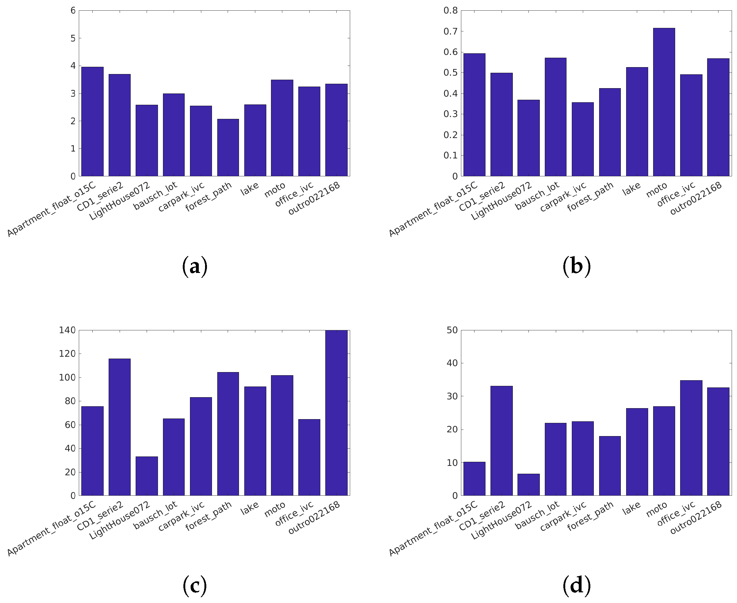
- Narwaria et al. [34]’s database (Available at http://ivc.univ-nantes.fr/en/databases/JPEG_HDR_Images/) is composed of 10 source images, which have been distorted by a backward compatible compression with the JPEG codec and the iCam TMO [36]. This database was used along with others to tune HDR-VDP2. The angular resolution used during the subjective test was 60 pix/degree and the surround luminance was 130 . For this database due to its surround luminance above 100 , we consider a surround luminance of 20 to obtain the color space . The characteristics of each reference image are reported on Figure 3.
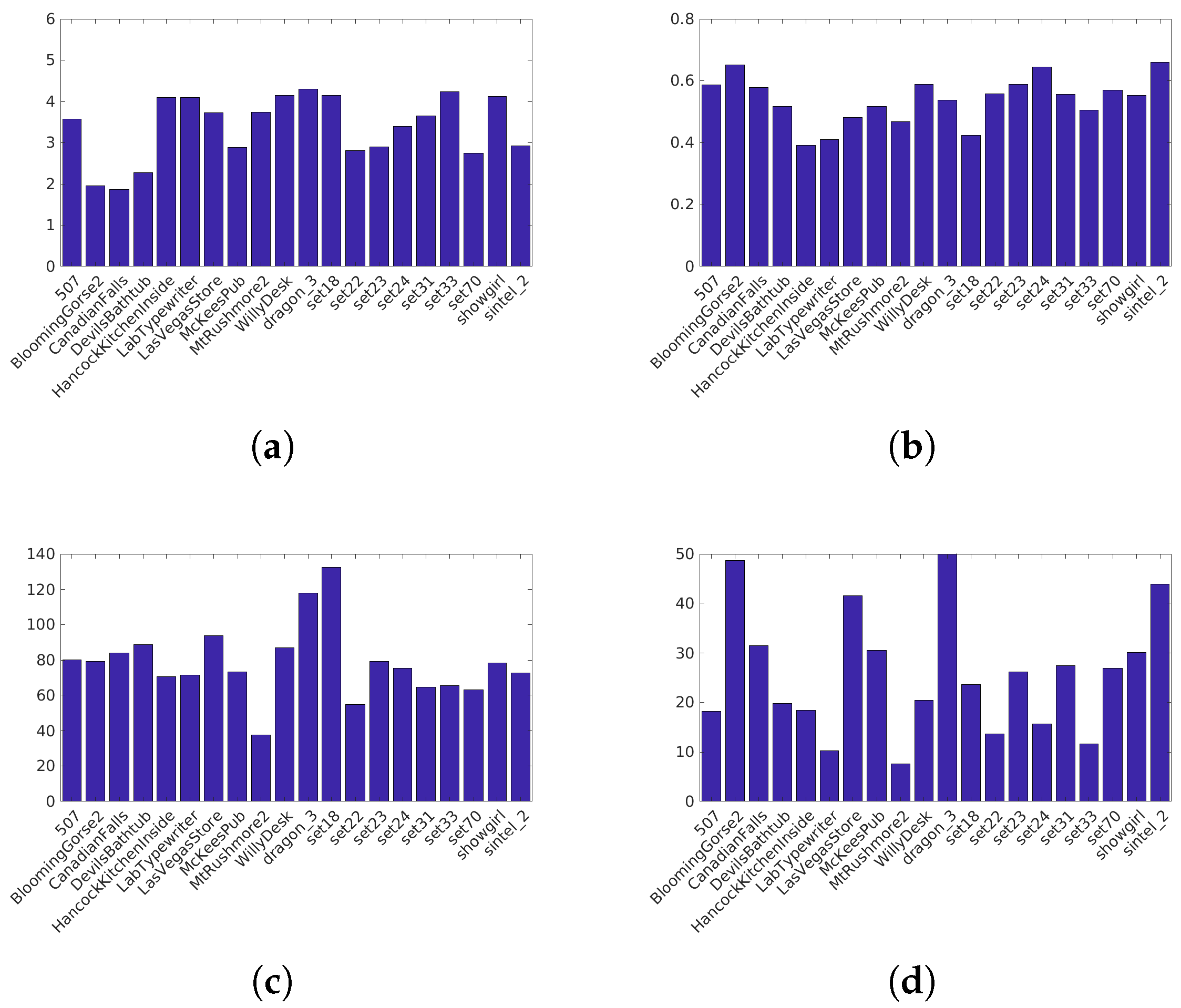
- Korshunov et al. [35]’s database (Available at http://mmspg.epfl.ch/jpegxt-hdr) consists in images distorted with a backward-compatible compression scheme using the JPEG-XT standard and either the Mantiuk et al. [37] or the Reinhard et al. [38] TMO. The angular resolution used during the subjective test was 60 pix/degree and the surround luminance was 20 . The characteristics of each reference images are reported on Figure 4.
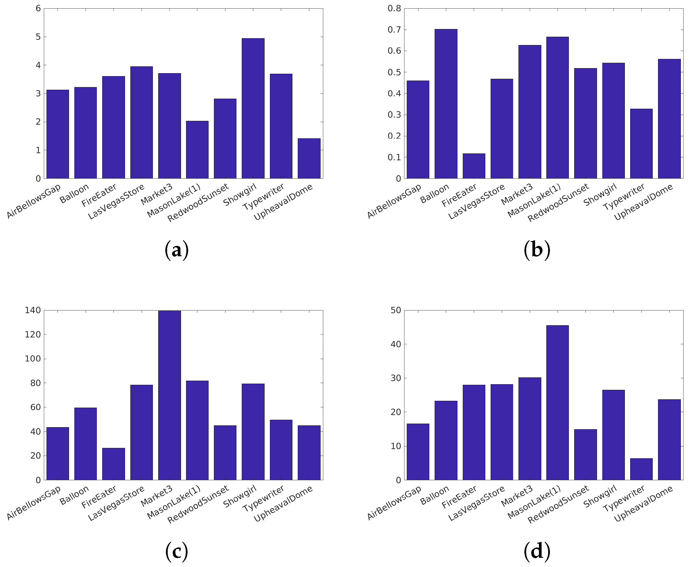
- Zerman et al. [19]’s database (Available at http://webpages.l2s.centralesupelec.fr/perso/giuseppe.valenzise/) is partially composed of images from [39]. The distorted images are generated by using both backward-compatible compression using the TMO proposed by Mai et al. [40] and using a non backward-compatible compression with the use of the PQ function for the EOTF. The compression was performed using the JPEG and the JPEG2000 codec. The angular resolution used during the subjective test was 40 pix/degree and the surround luminance was 20 . The characteristics of each reference images are reported on Figure 5.
The main limitation of these databases is the limited BT.709 gamut used during their creation. The wider BT.2020 color gamut is more and more associated with HDR images and videos. In addition, Standards Developing Organizations such as DVB, recommend the use of the BT.2020 gamut with HDR content [41].
3.1.2. Proposed Databases
To deal with the limitations of existing databases, we propose two new databases (Available at www-percept.irisa.fr/software/). The first one is a database with BT.709 contents encapsulated in a BT.2020 gamut and the second one is composed with native BT.2020 content. We used the same display for both of them: the SONY BVM-X300. This is a professional HDR video monitor able to faithfully display the brightness of signals [42]. It has a peak brightness at 1000 and a luminance of a black pixel that was too low to be measured by our equipment (<0.2 ). In this paper, we assume a luminance for the black pixel at 0.001 . This monitor also allows us to force the use of a chosen EOTF without having to consider the image metadata.
To display the images on the screen, we used the b<>com *Ultra Player* which allows to distribute uncompressed YUV content with a 10 bits quantization and 4:2:0 chroma sub-sampling.The connection to the screen was done using 3G-SDI cables.
To create the distortions, we used HDRTools (v0.16) (Available at https://gitlab.com/standards/HDRTools/) to apply format conversion, chrominance sub-sampling or gamut conversion. For the compression and decompression of the images, we used the reference software of HEVC, the HEVC test Model (v16.17) (Available at https://hevc.hhi.fraunhofer.de/).
For both subjective tests, we used the same methodology: the Double-Stimulus Impairment Scale (DSIS) variant I methodology [43] with a side-by-side comparison. Pairs of images were presented to the viewers, one side being always the reference. 50% of the participant had the reference always on the right-hand side, 50% always on the left-hand side. To avoid a bias with the order of presentation, the pairs of images were randomized for each participant with the condition that the same content was never shown twice consecutively. Each image pair was shown 10 s and voting time was 5 s. The test session lasts 35 min (including instructions and training time) with a 5 min pause in the middle of the test.
To obtain realistic distortion we compress the images with the HEVC codec using the recommendation ITU-T H Suppl.15 [44], i.e., a 10 bits quantization for the images, the PQ EOTF and the color space. Moreover this recommendation proposes different processes for increasing the quality of the compression such as a 4:2:0 chroma subsampling using a luma-adjustment process and a chroma Qp adaptation. This last is of special interest for this study because it corrects errors due to the compression of the chrominances. In WCG, most of chroma values tend to be near their mean value (i.e., 512) while the component tends to use most of its range. This is even more significant for BT.709 content encapsulated in a BT.2020 gamut. This behaviour creates a shift in the bitrate allocation from the chrominance to the luminance. This can potentially create visible chrominance artifacts. The chroma Qp adaptation proposed in the recommendation is a method to counter this effect. Because we wanted to create realistic color artifacts, we distort the images using the compression with and without the chroma Qp adaptation to study the sensibility of the color metrics.
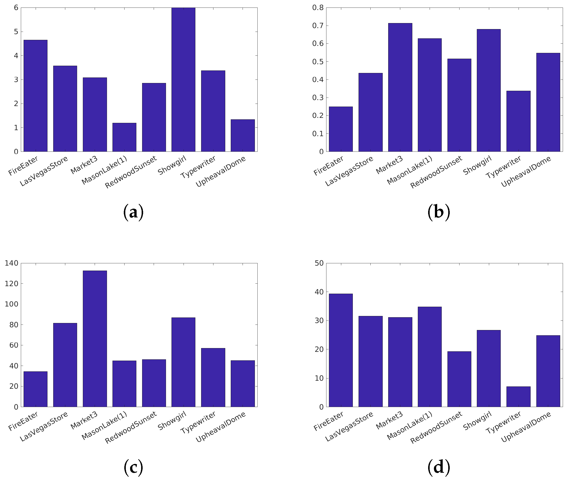
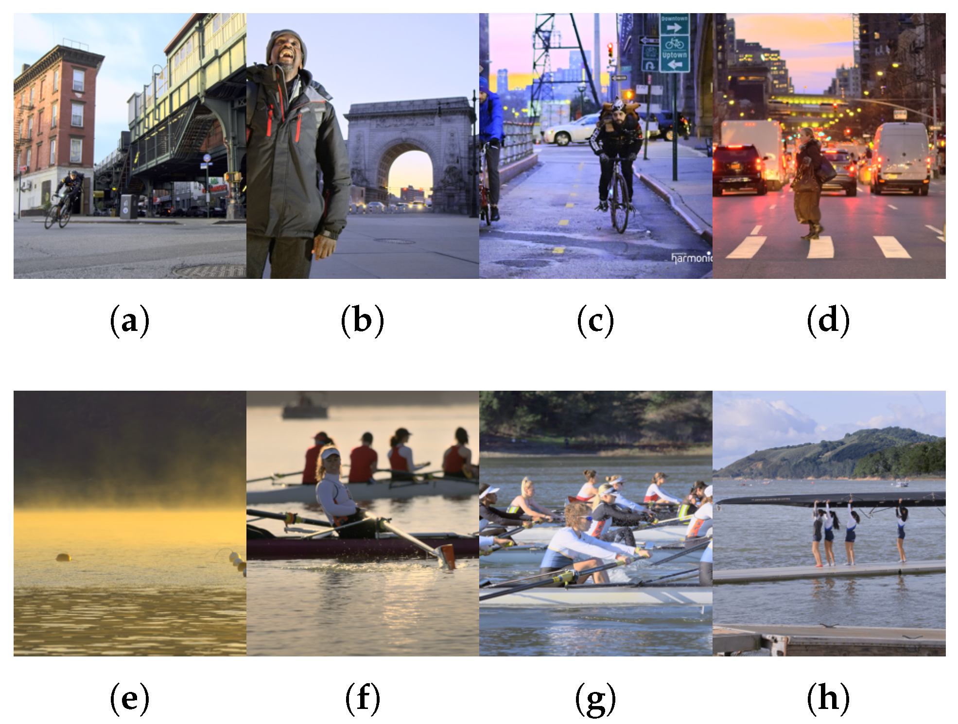
The first database we propose was already presented in [45]. Eight images were selected from 3 collections: two are from the MPEG HDR sequences (FireEater and Market) [46], one is from the Stuttgart HDR Video Database [47] and the remaining five images are from the HDR photographic survey [48]. Note that these images also belong to Zerman et al.’s database [19]. The characteristics of the images are not exactly the same as in Zerman et al. [19] because we used only half of the images () to be able to display simultaneously both the reference image and the distorted image on the same screen. The characteristics of the images can be found on Figure 6.
Fifteen naive subjects participated in this test (11 males, 4 females) with an average age of . All declared normal or corrected-to-normal vision. One participant was removed from the analysis using the methodology described in [43].
Because we used the display in HD mode, we choose to call this database HDdtb in this paper. Four kinds of distortions have been chosen:
- HEVC compression using the recommendation ITU-T H Suppl.15 [44]. Four different quantization parameters () were selected for each image for this distortion.
- HEVC compression without the chroma adaptation leading to more chrominance distortions. Three were selected for each image.
- Gaussian noise on the chroma components: 3 levels of noise were selected.
- Gamut mismatch: two kinds of distortion were created: on one hand, the BT.709 images were considered as if they had been already encapsulated in a BT.2020 gamut leading to more saturated images. On the other hand, we took images already encapsulated in a BT.2020 gamut and considered them as BT.709 images and re-encapsulated them in a BT.2020 gamut. This creates less saturated images.
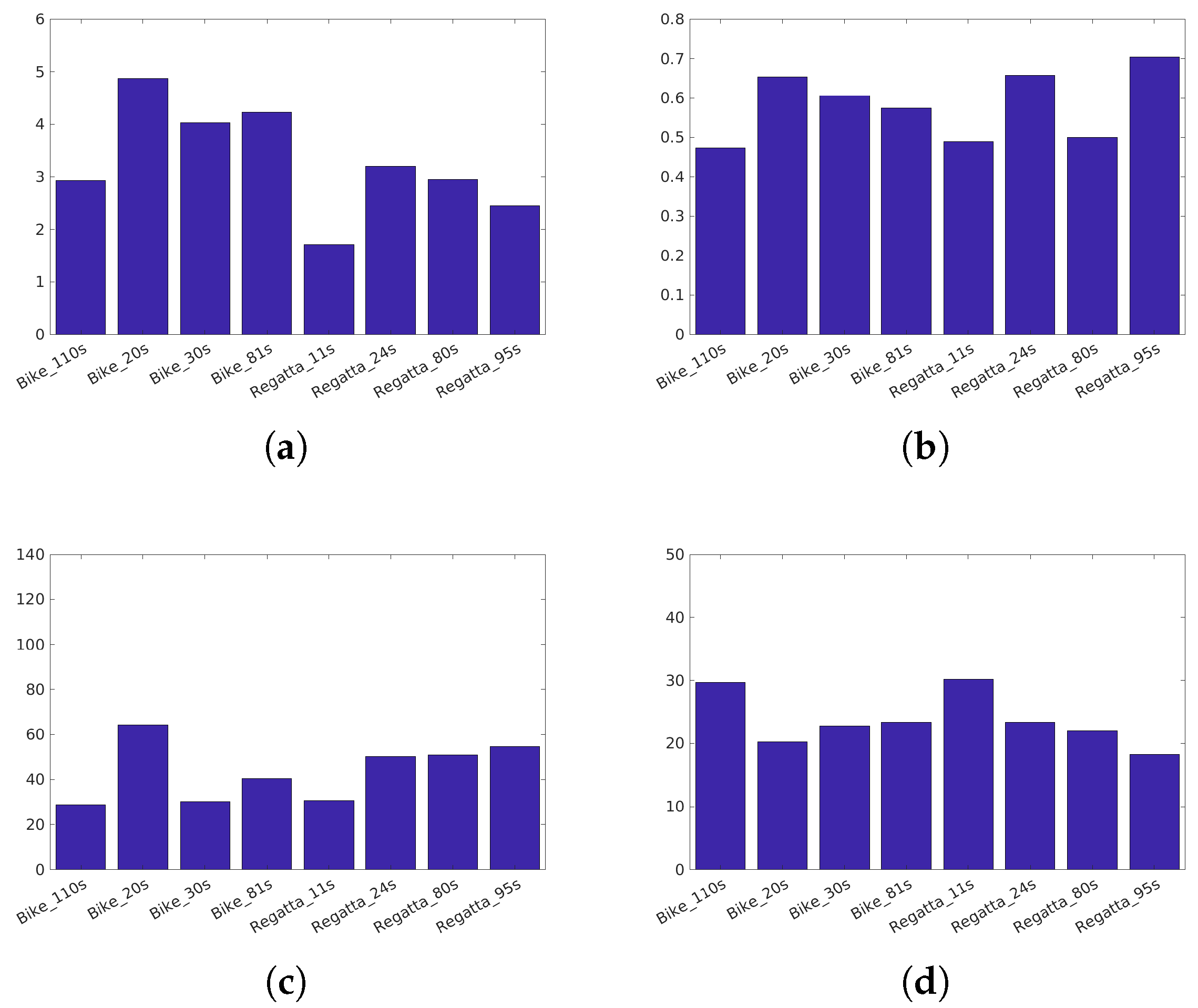
For the second database, we used eight 4K images produced by Harmonic Inc. The characteristics of the images are given in Figure 7. We used only part of these images so the reference and the distorted image could fit on our display () with a band of 60 black pixels. We called this new database 4Kdtb. We used the same visualization distance as in the previous database. Thirteen experts or sensitized subjects participated in this test (11 males, 2 females) with an average age of 40. All declared normal or corrected-to-normal vision. With this database we aim to create more visible color artifacts induced by compression than in the HDdtb database. We compressed the images with four different with three different options for the compression:
- HEVC compression using the recommendation ITU-T H Suppl.15 [44].
- HEVC compression without the chroma offset algorithm.
- HEVC compression with 8 bits quantization for the chroma instead of 10 during the compression. The chroma were re-sampled to 10 bits before displaying images on screen.
Because we have a higher resolution, the angular resolution increases as well and become 120 pix/degree. Because most quality metrics are not adapted to this kind of resolution, we choose to downsample the images to obtain a 60 pix/degree resolution before testing the different quality metrics. Using a downsampled image can improve the performances of some metrics such as MS-SSIM or HDR-VDP2, which were tuned for lower resolution.
3.2. Performance Indexes
We present the performances of the different quality metrics for each database with four different indicators. Before computing these indicators, a non linear regression is applied to the quality scores thanks to a logistic function:
where is the score of the quality metrics on the image i and the mapped quality score. Parameters a, b, c and d are determined by the regression conducted by the lsqcurvefit function of Matlab.
The four performance indicators are given below:
4. Results
In this section, we present the performances of the different metrics presented in the previous sections. For the sake of completeness, we also study the performances of the following color-blind HDR metrics: PU-VIF [9], HDR-VDP2 [11] (version 2.2.1) [12] and HDR-VQM [13]. Note that HDR-VDP2 requires a number of parameters such as the angular resolution, the surround luminance and the spectral emission of the screen. For these parameters, we use the values corresponding to the different subjective tests. We measured the spectrum of the Sony BVM-X300 and the SIM2 HDR47ES4MB monitor using the “X-Rite Eye one Pro 2” probe (more details are given in [45]. All these parameters are summarized in Table 3.
Figure 8, Figure 9, Figure 10, Figure 11 and Figure 12 represent the SROCC performances for each database and each metric. Numerical values of the performance indexes (SROCC, PCC, OR, RMSE) can be found in Appendix B.
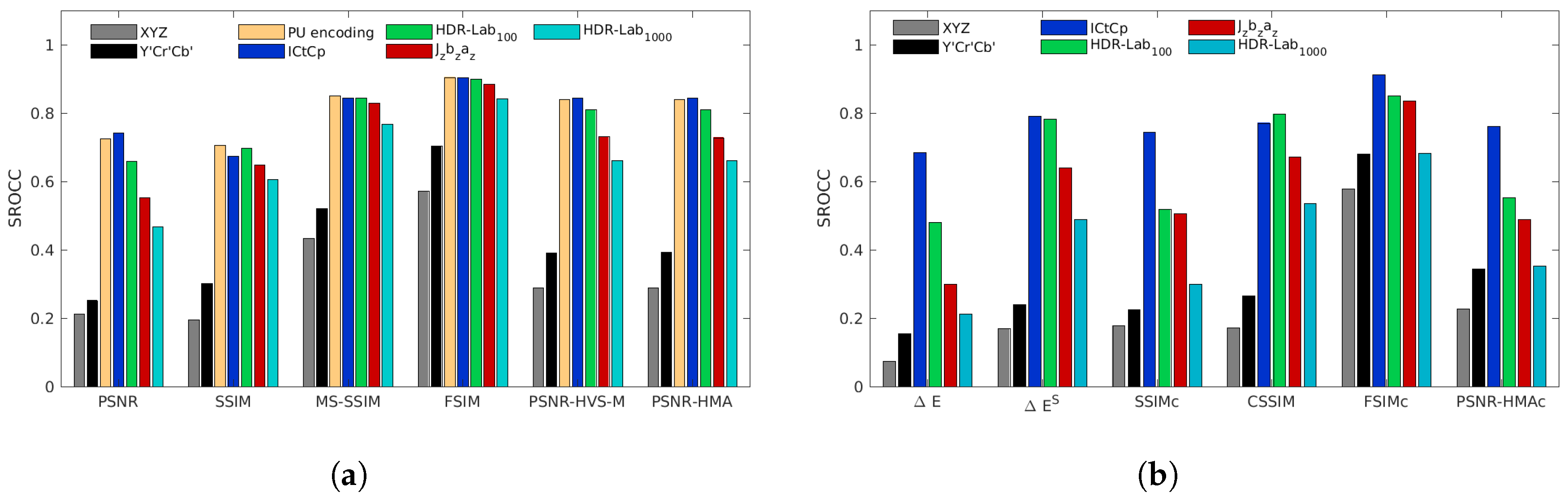
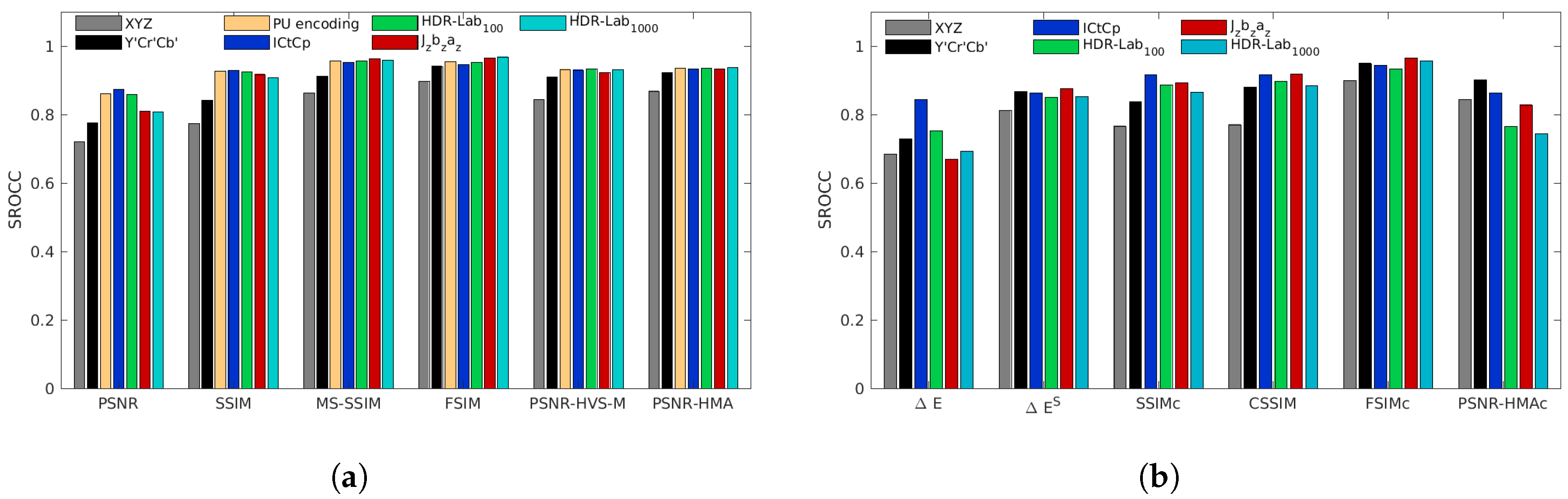
4.1. 4Kdtb Database
With our proposed 4Kdtb (cf. Figure 8), for each color-blind metrics, the best color spaces are always the , and the PU-encoding. and provide the lowest performances. The best performing color-blind metrics is FSIM used with the PU-encoding, closely followed by and . MS-SSIM used with the PU encoding, and, are almost on par with the second best performing metrics HDR-VDP2 (cf. Appendix B). The only color space that provides good performances on all color metrics is the color space.
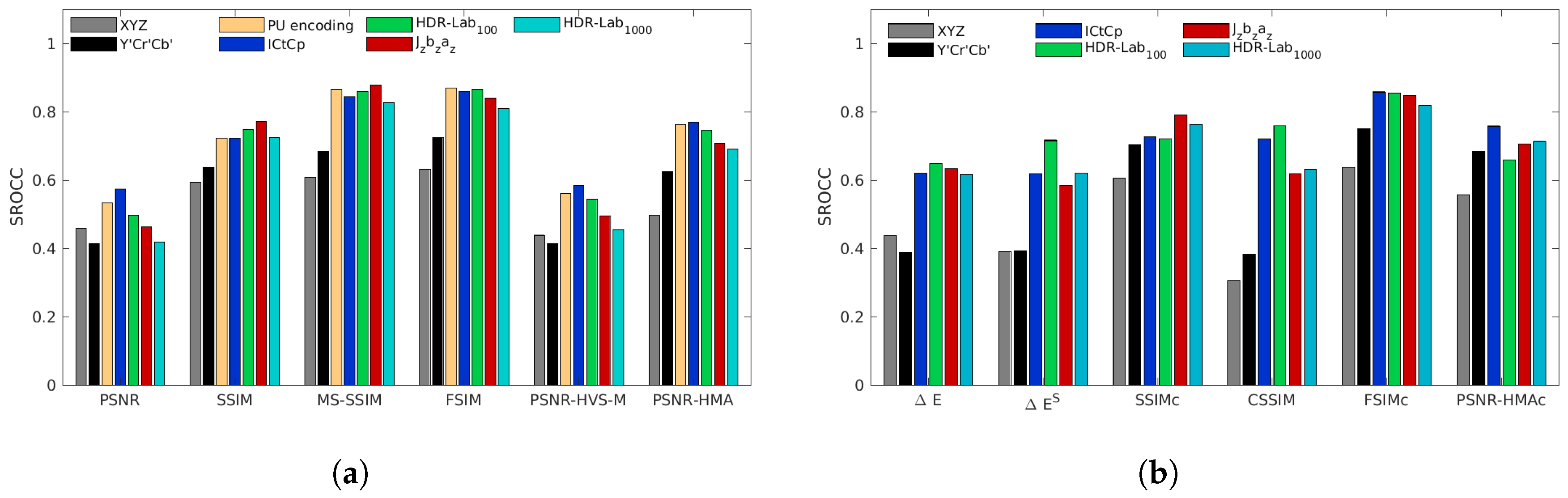
4.2. Zerman et al. Database
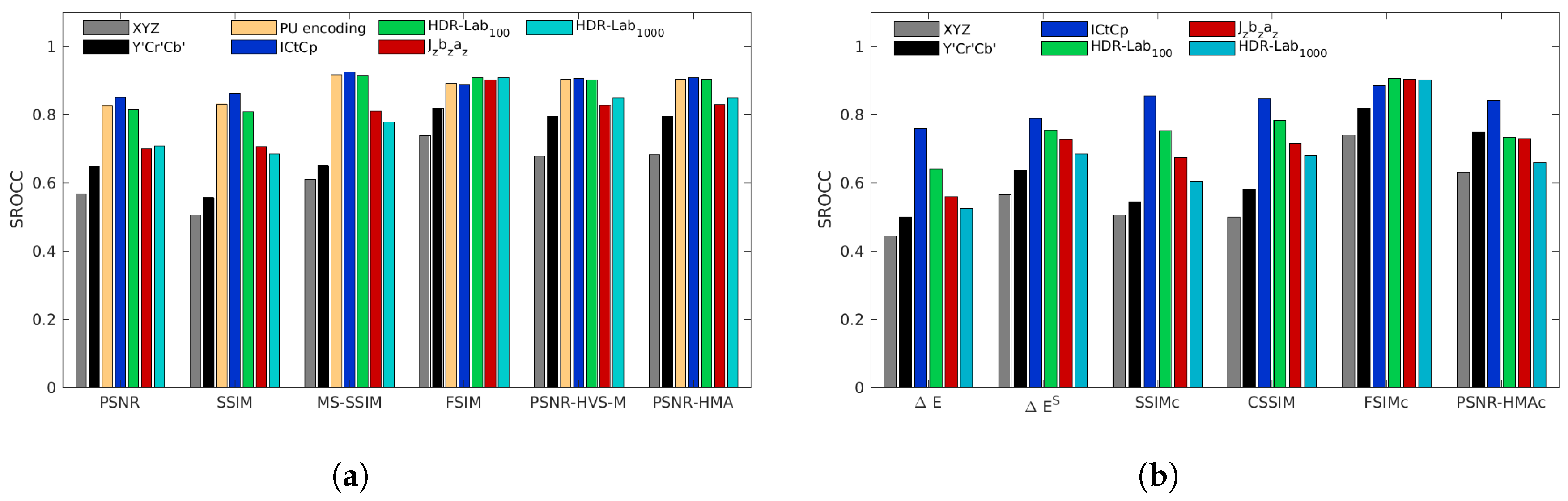
With the Zerman et al. database, as previously, the color spaces, , and the PU-encoding provide the best performances for almost all color-blind metrics (cf. Figure 9). However, there is one exception with FSIM. Used with the following color spaces, , and , it provides slightly better performances than and the PU-encoding. The best performing color-blind metrics are, with almost the same performances, HDR-VDP2, HDR-VQM and .
4.3. HDdtb Database
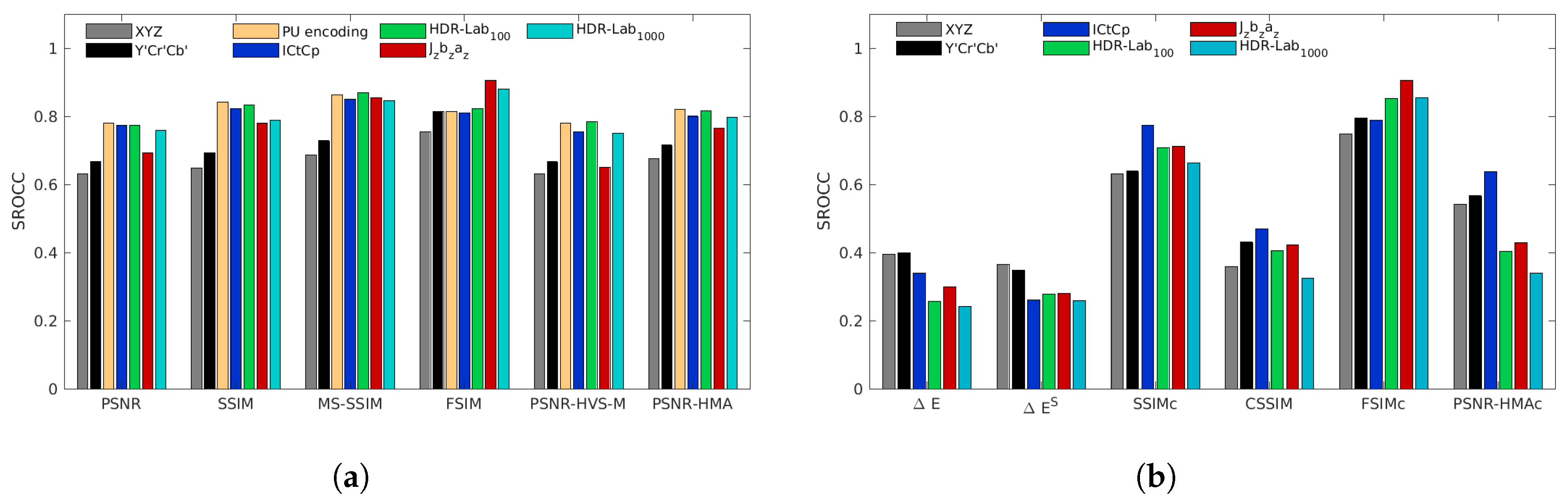
With our proposed HDdtb (cf. Figure 10), for color-blind metrics, the color space provides slightly lower performances for all metrics, except with FSIM. For this metric, the performances with are higher. The best performing color-blind metrics for this database are , and . For the color metrics, the metrics based on color difference metrics (, and CSSIM) have very low performances. This is partially due to the presence of the gamut mismatch artifact. As noticeable on Table 4, discarding this artifact increases the performances of these metrics. For the participants of our subjective test, the distortions on the images are clearly visible but are not directly associated with a loss in quality perception.
4.4. Korshunov et al. Database
The Korshunov et al. database is the less selective database (cf. Figure 11). Most of the metrics have high correlation coefficients and the choice of color space has close to no impact on the performances especially on color-blind metrics. Even using non-perceptually linear color space like the color space impacts only moderately the performances of MS-SSIM, FSIM, PSNR-HVS-M and PSNR-HMA. For this database, the best performing color-blind metrics are , and .
4.5. Narwaria et al. Database
With the Narwaria et al. database (cf. Figure 12), is the best color space for SSIM and MS-SSIM while the PU-encoding and the are the best color spaces for FSIM. The best metrics for this database are , HDR-VDP2 and HDR-VQM. The good performances of HDR-VDP2 were expected for this database because it was part of the training set of this metric. For this database, the performances of the PSNR and the PSNR-HVS-M are relatively low compared to the other databases. The fact that PSNR-HMA with the adequate color space significantly increases the performances of PSNR-HVS-M suggests that the backward compatible compression used by Narwaria et al. (Section 3.1.1) creates distortions that impact the mean luminance and the contrast of the images. Indeed PSNR-HMA is an improvement of PSNR-HVS-M that takes into account these two kinds of artifacts [50].
4.6. Results Summary
For all studied databases, HDR-VDP2 has generally high performances although it is not always on the top three metrics (cf. Appendix B). FSIM and MS-SSIM with appropriate perceptually uniform color space are often on par if not better than HDR-VDP2.
Among all metrics, FSIM is the less sensitive metrics to the choice of color space assuming that this color space is perceptually uniform.
The color extension of FSIM, namely FSIMc, does not improve the performances of FSIM even for our proposed database 4Kdtb which focuses on chromatic distortions. Worst, the metrics becomes much more sensitive to the color space choice. We observe the same behavior for the color extension of PSNR-HMA, PSNR-HMAc, which decreases the performances of the metrics for any color spaces.
When using the two non-uniform color space and , the performances of all metrics drop significantly compared to the other color spaces for all the databases and especially for our proposed database 4Kdtb, the Zerman et al. database and the Narwaria et al. database. It emphasizes the importance of perceptually uniform color space for predicting the quality of HDR images.
5. General Discussion
We separate our general discussion in two parts. First, we study the impact of the color space on the metrics performances. Moreover we emphasize the influence of the diffuse white luminance. As a reminder, the luminance of the diffuse white correponds to the luminance of a 100% reflectance white card without any specular highlight. In HDR imaging, it is different from the peak brightness. In the second part of our analysis, we discuss the sensitivity of chrominance artifacts on color metrics using our proposed database 4Kdtb.
5.1. Impact of the Diffuse White Luminance
Our results suggest that the best color space for assessing the quality of HDR images depends on the test database. Indeed, some of the color spaces are adapted and tuned for one visualization condition.
The color space considers two important parameters, i.e., the diffuse white and the surround luminance. Moreover, the final equation of the color space (Equation (13)) was tuned using the experimental dataset called SL2 [20]. This dataset was obtained for a diffuse white at 997 . This explain why the luminance have a behaviour close to the luminance (cf. Figure 2).
The PU function and the color space were not obtained through the same kind of training. They were created using Daly’s Contrast Sensitivity Function model [51] and Barten’s Contrast Sensitivity Function model [52], respectively. However, Figure 2, that represent the different color spaces luminance in function of the linear luminance, suggest that and the PU encoded luminance have a behaviour closer to the luminance than from the luminance or than the luminance.
Because the color spaces are adapted for different viewing conditions, it is not easy to determine the best color space.
- With the proposed database 4Kdtb, the color spaces with a diffuse white around 100 (, and the PU-mapping) give better performances than and spaces. We also observe that the performances of color metrics are more sensitive to the color space choice.
- We draw a similar conclusion on Zerman et al. database, except for FSIM and FSIMc (cf. Figure 9). These two metrics are less sensitive to the color space for this database.
- With the proposed database HDdtb (cf. Figure 11), the color space provides the lowest performances for PSNR, SSIM, MS-SSIM and PSNR-HMA metrics but provides the highest performances with FSIM and FSIMc. However, results indicate that the PSNR, SSIM and PSNR-HMA metrics based on and color spaces perform better than the same metrics using the color space. This suggests that the low performances of these metrics is not due to the diffuse white characteristics of the images, but to the design of color space which corrects a deviation in the perception of the blue hue (cf. Equation (9)). To test this hypothesis, we measure the SROCC of these metrics on the HDdtb database with the color space without the blue deviation correction. We call this new space . Results, shown in Table 5, indicate that SROCC values of the three aforementioned metrics increase with the color space. In addition, metrics using this modified color space provide similar performances to metrics based on the color space. This is consistent with the fact that and are adapted to almost the same diffuse white luminance. This might be due to the presence of the “gammut mismatch” artifact in this database. Indeed, the “gammut mismatch” artifact creates visible distortions that was not associated with a subjective quality loss during our test. We suspect that the blue hue deviation correction makes the color space more sensitive to this distortion. However, this is difficult to demonstrate due to the low number of images with this kind of artifact present in this database.
- With the Narwaria et al. database, it is difficult to draw a conclusion (cf. Figure 12). The MS-SSIM and the SSIM metrics perform better when using the color space. However, the FSIM and PSNR-HMA metrics perform better when using the color space. This contrasted result might be due to the fact that the diffuse white luminance is likely not homogeneous across the entire database.
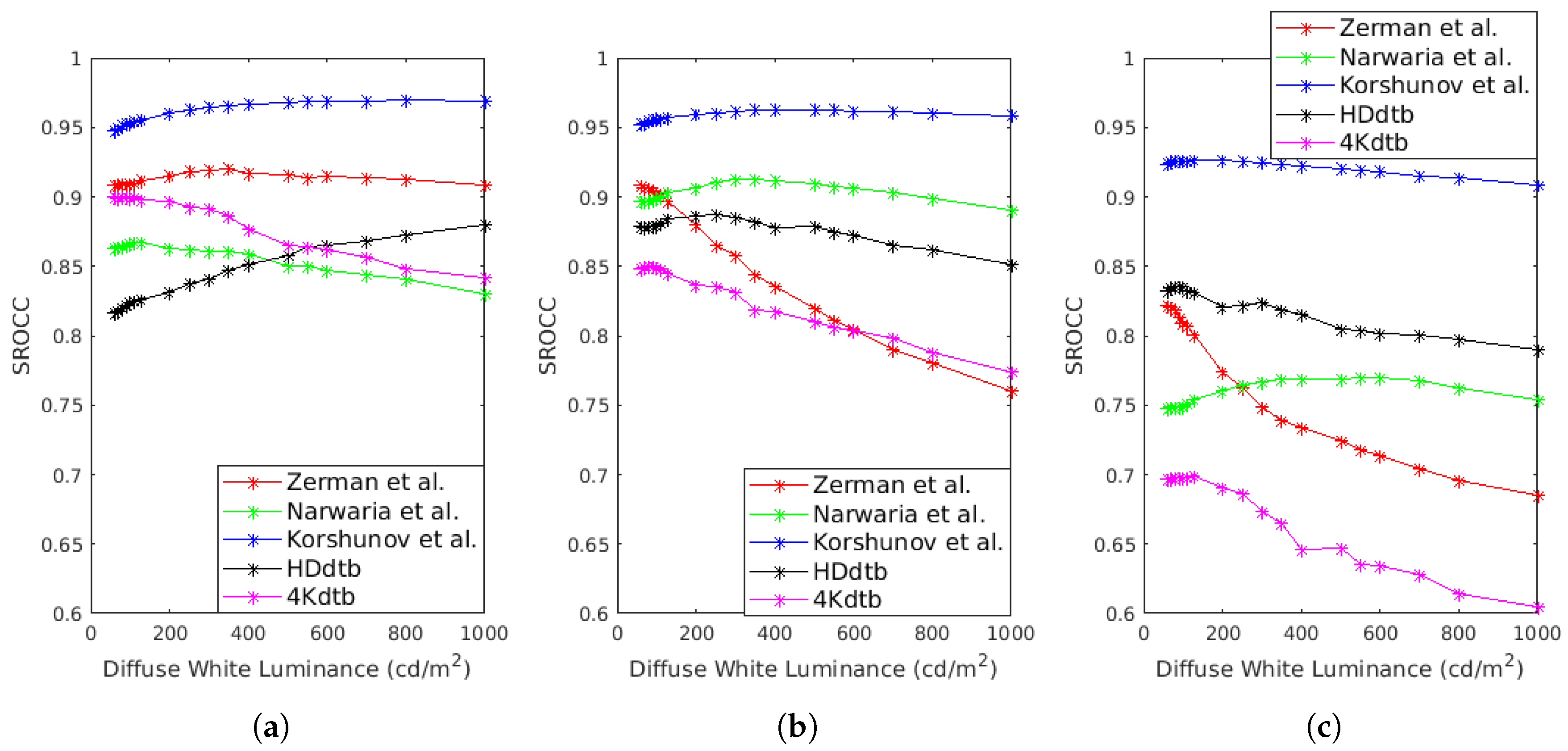
To go further into the analysis, we propose to evaluate the impact of the diffuse white on the performances of metrics. The SROCC performances of three metrics (FSIM, MS-SSIM and SSIM) are evaluated for a diffuse white in the range 80 to 1000. Results are plotted in Figure 13. For the FSIM, the performances decrease slightly when the diffuse white luminance increases for the 4Kdtb database and the Narwaria et al. database while increasing with the diffuse white for the HDdtb. The impact of the diffuse white is more important on the MS-SSIM metric. For example, with the Zerman et al. database, the SROCC score drops from 0.9143 to 0.7791. The impact for the SSIM metrics is in the same order of magnitude as for MS-SSIM.
5.2. Sensibility to Chrominance Distortions
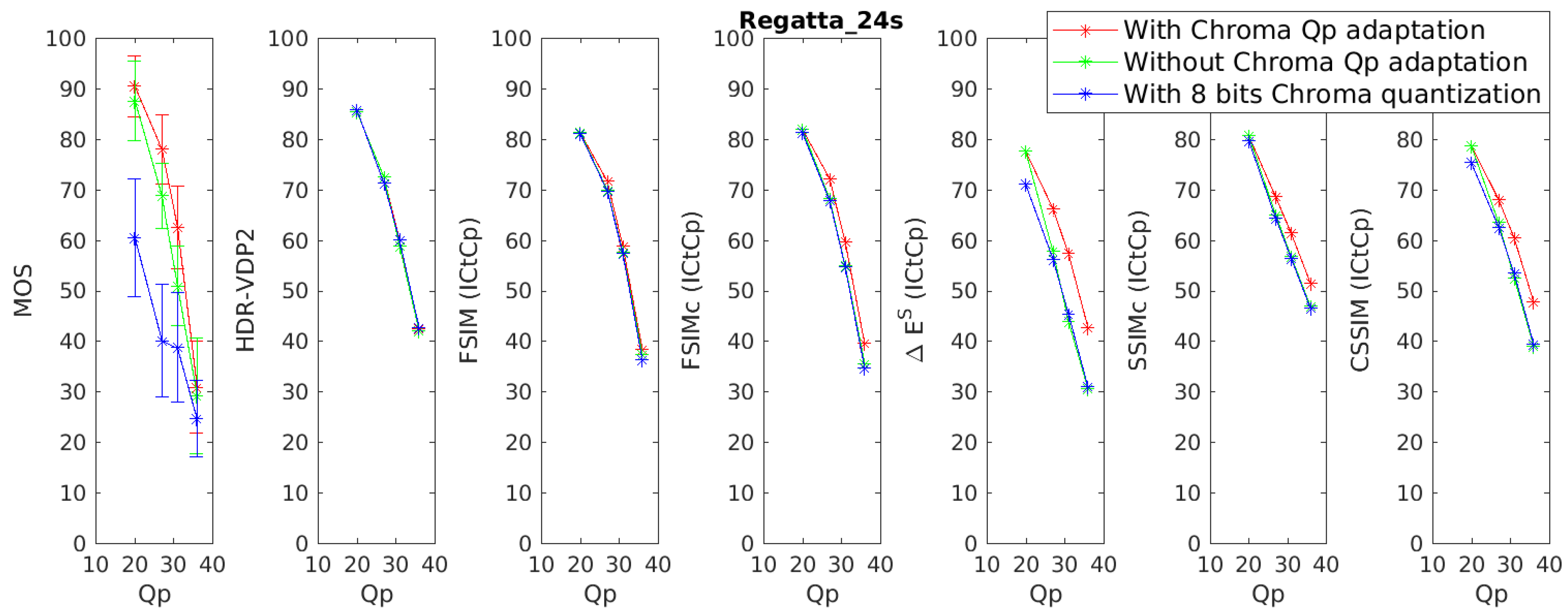
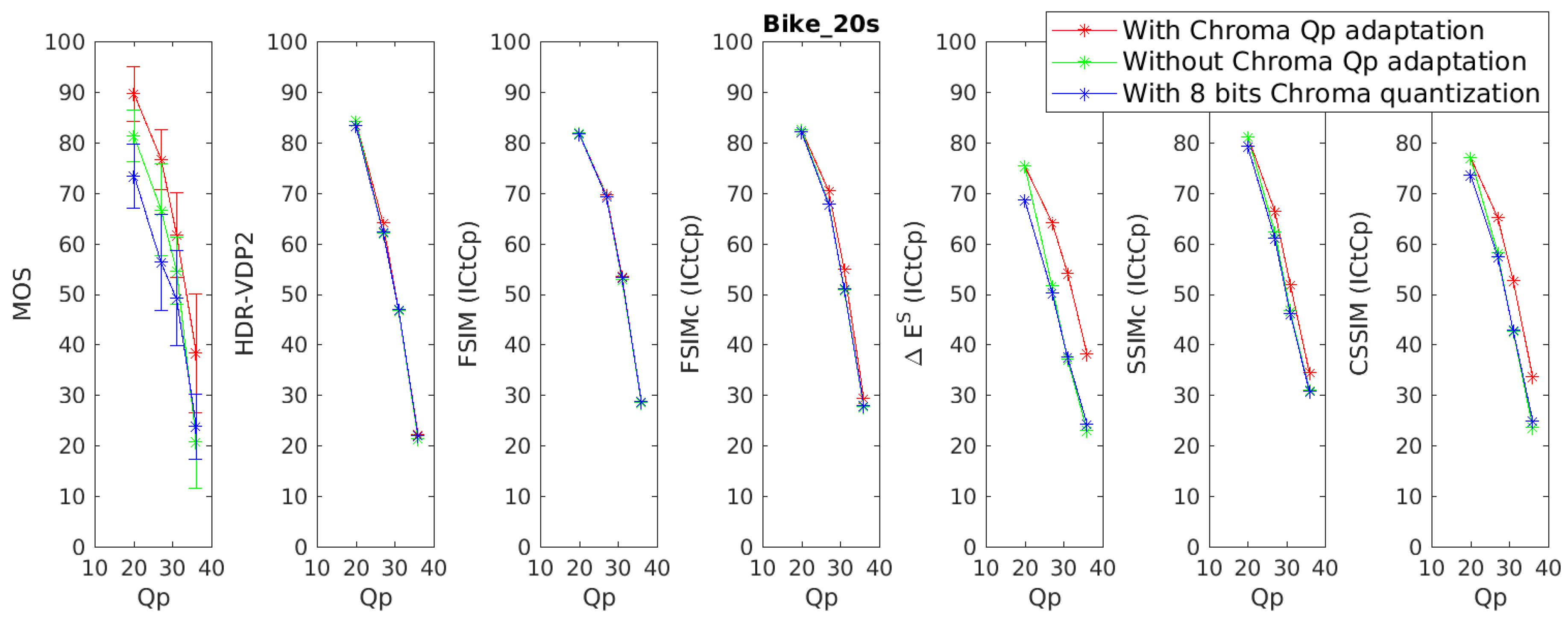
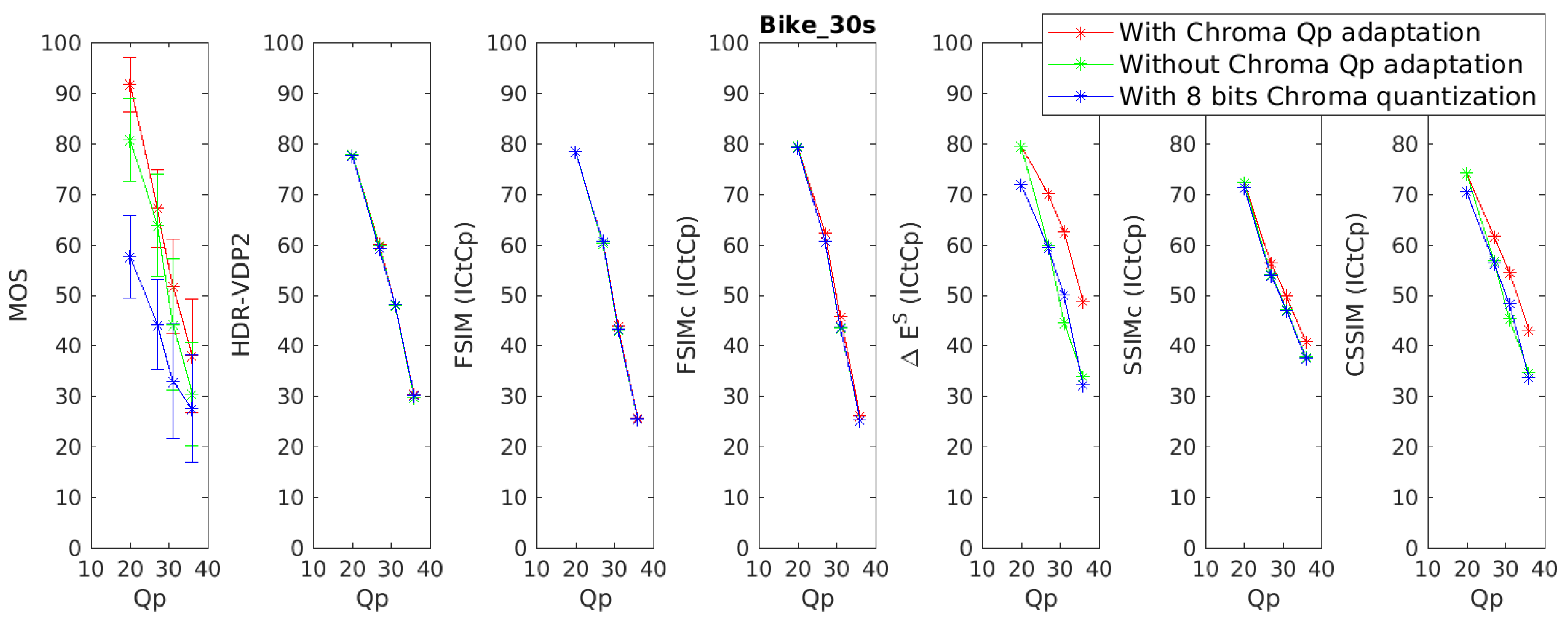
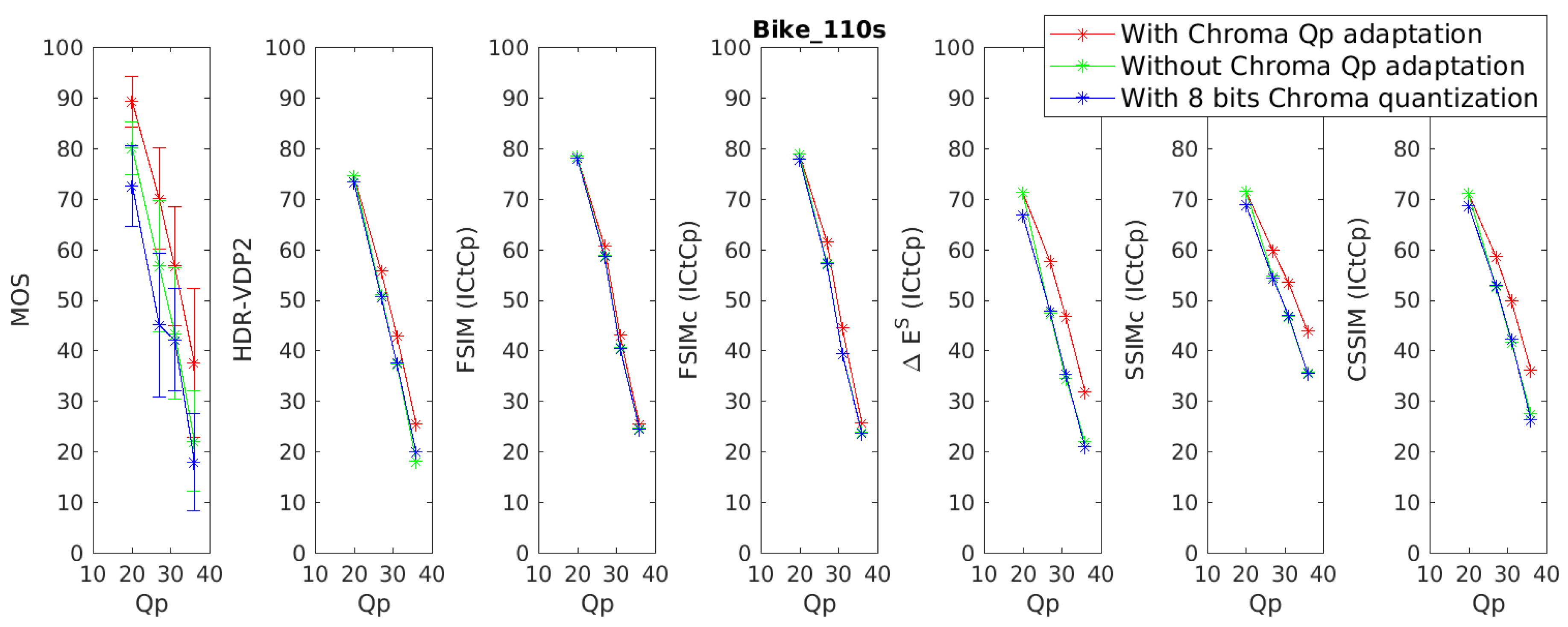
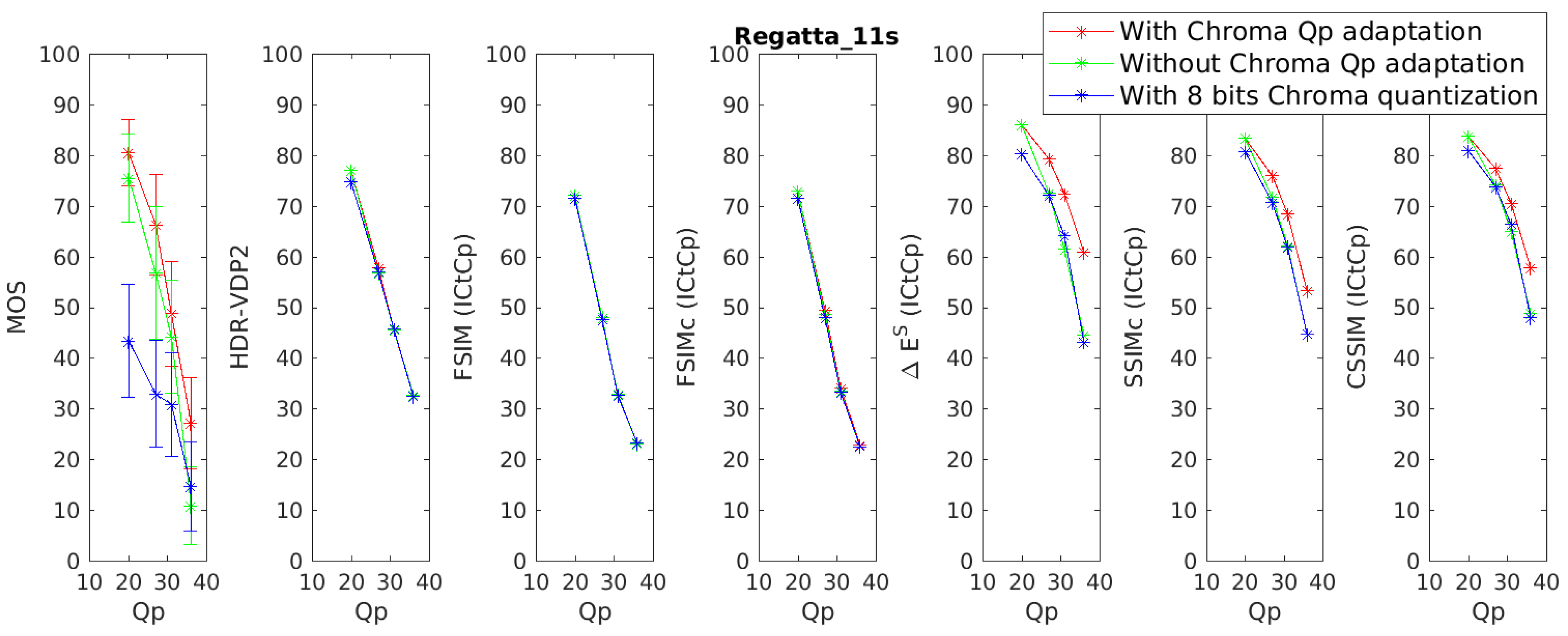
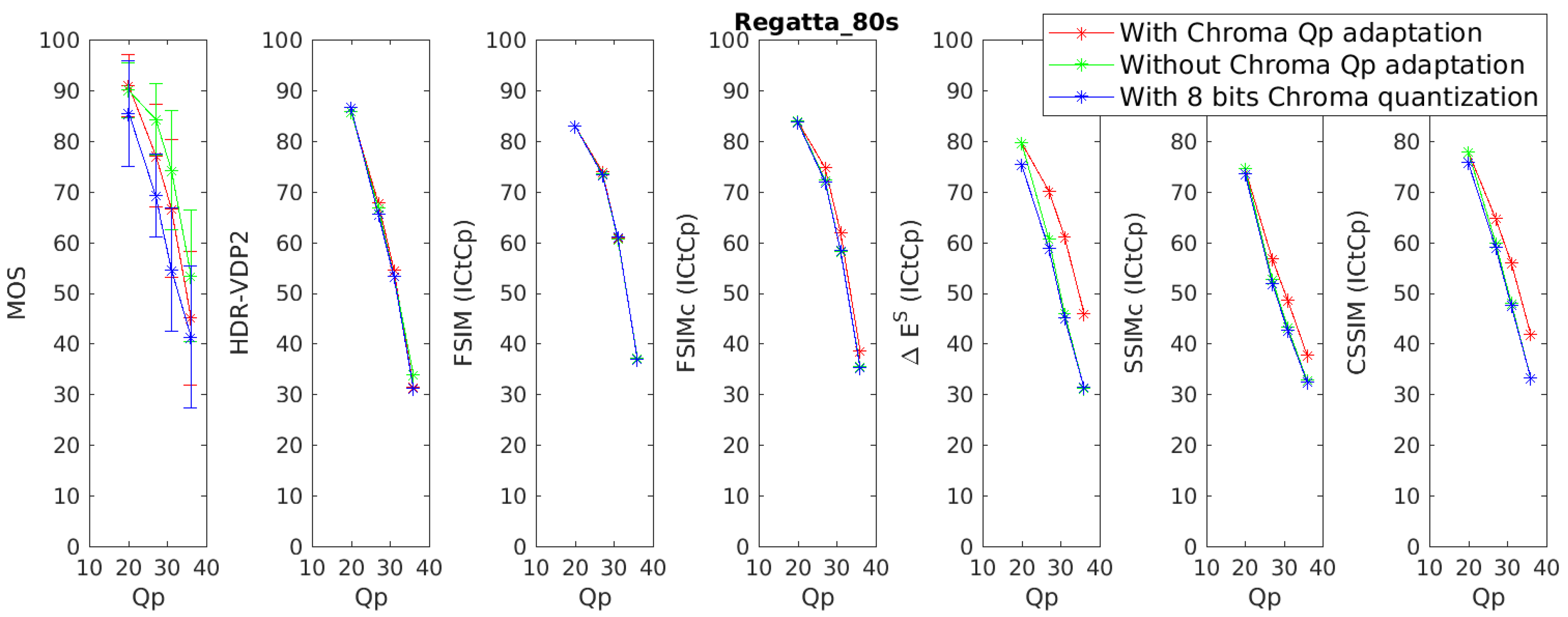
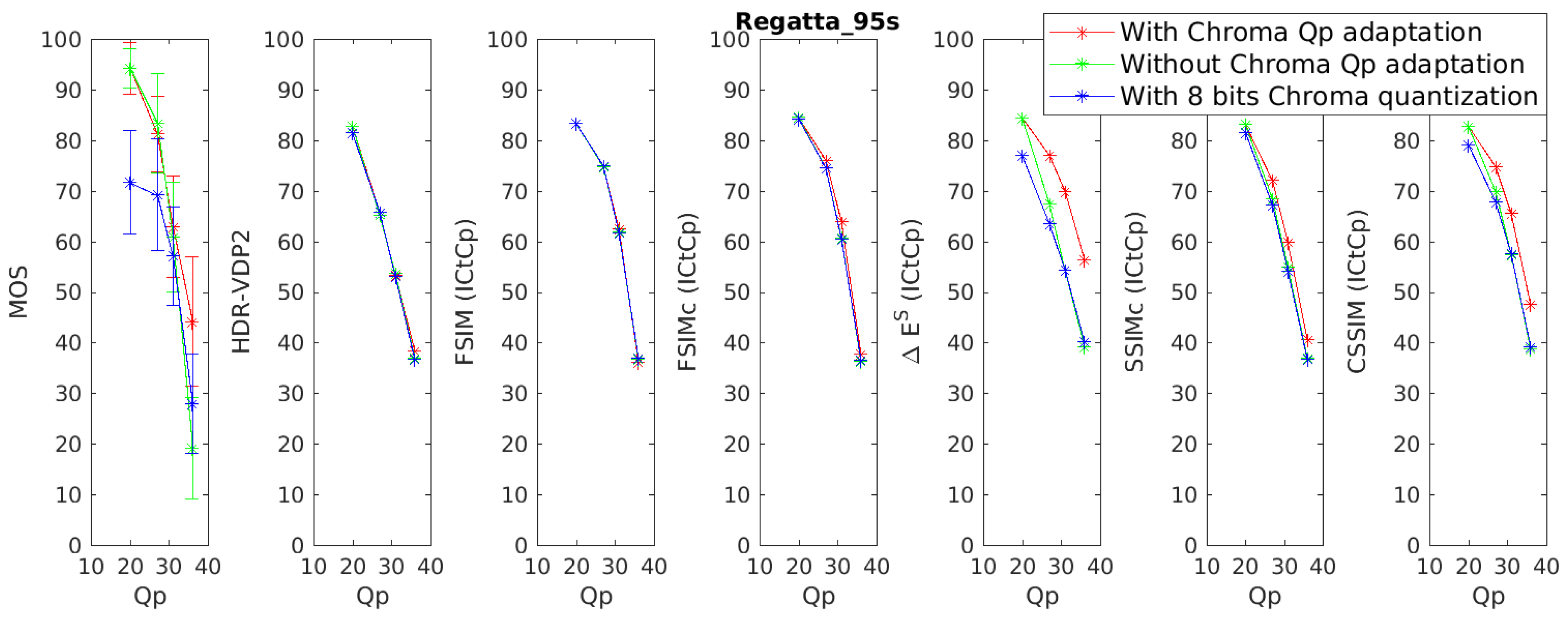
In this section, the ability of color metrics to take into account chrominance artifacts is discussed. The discussion is focused on the database 4Kdtb which is the only database providing significant chrominance artifacts. Also we only consider metrics using the color space since the best performances are observed with this color space. Figure 14 presents the Mean Opinion Score (MOS) and objective scores for the reference image “Regatta_24s”, for the distorted images (compressed with HEVC). The objective scores are given after applying the logistic regression presented in Section 4. Results for the other reference images can be found on Appendix C.
There is a clear difference of quality perception between the images compressed with the chroma adaptation (cf. Section 3.1.2) (red Line) and the images compressed without the chroma adaptation and a 8 bits quantization on the chrominance (blue line). The MOS of images compressed without the chroma adaptation algorithm and a 10 bits quantization (green line) are in-between the two previous encodings.
As expected, the color-blind metrics, i.e., HDR-VDP2 and FSIM, are not sensitive at all to the chrominance distortions. However, more surprisingly, the color extension of FSIM, namely FSIMc, is not sensitive to the generated chrominance artifacts. The metrics was tailored for images in a BT.709 gamut with a SDR range. Its non-sensibility to the chrominance might be due to the pre-defined constant used for the color comparisons [29].
The other color metrics, i.e., , SSIMc and CSSIM, are more sensitive to the chrominance artifacts. However, SSIMc and CSSIM have a tendency to underestimate the influence of chrominance artifacts for images compressed with a low (so low distortion in the luminance channel) and a 8 bits quantization on the chrominance (cf. Figure A7, Figure A9, Figure A10, Figure A11 and Figure A13).
6. Recommendations
In this section, some recommendations are given to assess the HDR/WCG content quality in the context of image/video compression. The recommendations are listed below:
- For assessing the impact of luminance distortions, we recommend to use the FSIM metric. This is one of the best performing metrics. Moreover, it is the less sensitive to the choice of color space and to the diffuse white of the images. Using the color extension of the metrics (FSIMc) does not bring a significant added-value. In addition, it is important to underline that the FSIMc metrics is sensitive to the choice of color space (cf. Figure 8).
- For assessing the impact of chrominance distortions, we recommend to use the metric.
- For assessing the impact of both luminance and chrominance distortions, we recommend to use both the FSIM metrics and the metrics.
- To choose the color space, we recommend to take into account the diffuse white used during the color grading of the images. If the producer of the content follows the ITU recommendation BT.2408 [53] that defines the diffuse white luminance at 203 , we recommend to use the color space. Indeed, this color space is well adapted to a low value of diffuse white. At the opposite, the color space is well appropriate for a diffuse white luminance at 997 . Another benefit to use the color space is related to its direct compatibility with popular compression codecs such as HEVC.
- For application where the calculation time and the complexity are critical aspects, we recommend to be very careful with the choice of the color space. The simplest metrics, such as PSNR and SSIM, are much more sensitive than FSIM to the diffuse white luminance.
- If the chosen metrics is the PSNR, we recommend to first verify that the tested image/video processing application, such as compression codecs, does not create luminance mean shift or contrast change. These artifacts can be induced by backward compatible compression (if the image is first tone-mapped, then compressed using a legacy codec and finally tone expanded).
Due to the characteristics of the tested databases, these recommendations have to be used in the context of image/video compression. Different subjective tests would be required to extend the analysis to other kinds of distortion.
7. Conclusions
In this article, we reviewed the relevance of using SDR metrics with perceptually uniform color spaces to assess the quality of HDR/WCG contents. We studied twelve different metrics along with six different color spaces. To evaluate the performances of these metrics, we used three existing HDR image databases annotated with MOS and created two more databases specifically dedicated to WCG and chrominance artifacts. We showed that the use of perceptually uniform color spaces increases, in most cases, the performances of SDR metrics for HDR/WCG contents.
In this study, we also highlight two weaknesses of state-of-art metrics. First, The relationship between the diffuse white used for grading the image and the diffuse white used for the color space is not always easy to define. In a number of cases, we do not know the value of the diffuse white used for grading of the image. Choosing an arbitrary diffuse white for the color space may significantly alter the objective quality assessment. Further analysis of this relationship is required. A better understanding could help to evaluate compression of images using the HLG EOTF for which the diffuse white depends on the display. Second, to the best of our knowledge, the quality assessment of DR/WCG images with chrominance distortions is still an open-issue, because of the lack of relevant objective metrics.
In a broader perspective, the relevance of subjective tests can also be questioned. For example, on the proposed database HDdtb, viewers did not perceive the gamut mismatch artifact as a loss of quality. However, this kind of artifact changes completely the appearance of images. Some other artifact could also alter the image appearance like the tone mapping/tone expansion used during backward compatible compression. In some cases, asking the viewers to not assess only the quality of the images but also their fidelity to the image appearance can be valuable to fully evaluate image processing algorithms.
Supplementary Materials
The following are available online at https://0-www-mdpi-com.brum.beds.ac.uk/2313-433X/5/1/18/s1.
Author Contributions
Conceptualization, M.R.; Data curation, M.R.; Formal analysis, M.R.; Investigation, M.R.; Methodology, M.R.; Project administration, O.L.M., R.C. and X.D.; Resources, M.R., O.L.M., R.C. and X.D.; Software, M.R.; Supervision, O.L.M., R.C. and X.D.; Validation, O.L.M., R.C. and X.D.; Writing—original draft, M.R.; Writing—review & editing, O.L.M., R.C. and X.D.
Funding
This research received no external funding.
Acknowledgments
Thanks to all the participants that have accepted to be part of the two proposed subjective tests.
Conflicts of Interest
The authors declare no conflict of interest.
Abbreviations
The following abbreviations are used in this manuscript:
| HDR | High Dynamic Range |
| SDR | Standard Dynamic Range |
| WCG | Wide Color Gamut |
| HVS | Human Visual System |
| EOTF | Electro-Optic Transfer Function |
| OETF | Opto-Electronic Transfer Function |
| PU | Perceptually Uniform |
| PQ | Perceptual Quantizer |
| HLG | Hybrid Log Gamma |
| CSF | Contrast Sensitivity Function |
| DSIS | Double-Stimulus Impairment Scale |
| ACR-HR | Absolute Category Rating with Hidden Reference |
| SI | Spatial Information |
| DR | Dynamic Range |
| SROCC | Spearman Rank Order Correlation Coefficient |
| PCC | Pearson Correlation Coefficient |
| OR | Outlier Ratio |
| MSE | Mean Square Error |
| RMSE | Root Mean Square Error |
| PSNR | Peak Signal on Noise Ratio |
| SSIM | Structure SIMilarity |
| MS-SSIM | MultiScale Structure SIMilarity |
| FSIM | Feature SIMilarity |
| VIF | Visual Information Fidelity |
| HDR-VDP | High Dynamic Range Visual Difference Predictor |
| HDR-VQM | High Dynamic Range Video Quality Metric |
| TMO | Tone Mapping Operator |
| JPEG | Joint Photographic Experts Group |
| HEVC | High Efficiency Video Coding |
| ITU | International Telecommunication Union |
| DVB | Digital Video Broadcasting |
Appendix A. Database Images
The following images represent tone map version of all the used reference images. The tone mapping operator (TMO) used to produce this images was the Reinhard et al. TMO [54]. We used its Matlab implementation of the HDRToolbox [55]. The reason why the same content present in several databases (like FireEater) can have a different rendering is because the Reinhard TMO was applied indifferently on BT.709 content and BT.2020 content.
Appendix A.1. Narwaria et al.
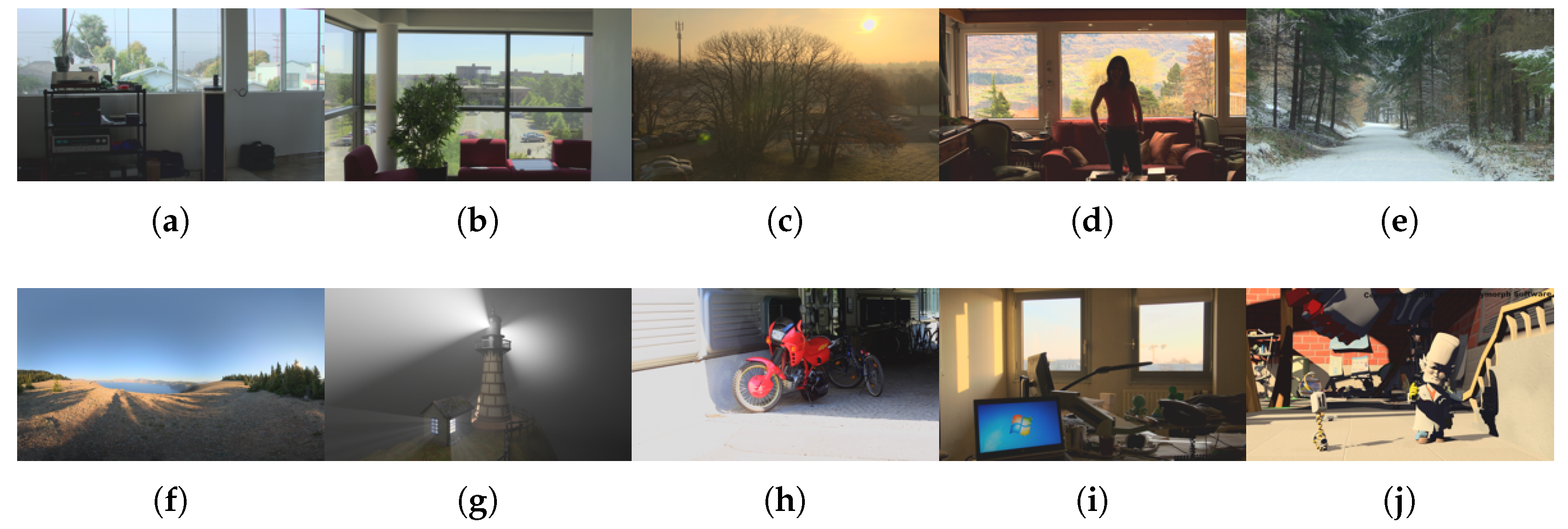
Figure A1.
Tone-mapped version (Reinhard et al. TMO [54]) of Narwaria et al. reference images. From left to right and from top to bottom: (a) Apartment_float_o15C (b) bausch_ lot (c) carpark_ ivc (d) CD1_serie2 (e) forest_path (f) lake (g) LightHouse072 (h) moto (i) office_ivc (j) outro022168.
Figure A1.
Tone-mapped version (Reinhard et al. TMO [54]) of Narwaria et al. reference images. From left to right and from top to bottom: (a) Apartment_float_o15C (b) bausch_ lot (c) carpark_ ivc (d) CD1_serie2 (e) forest_path (f) lake (g) LightHouse072 (h) moto (i) office_ivc (j) outro022168.

Appendix A.2. Zerman et al.
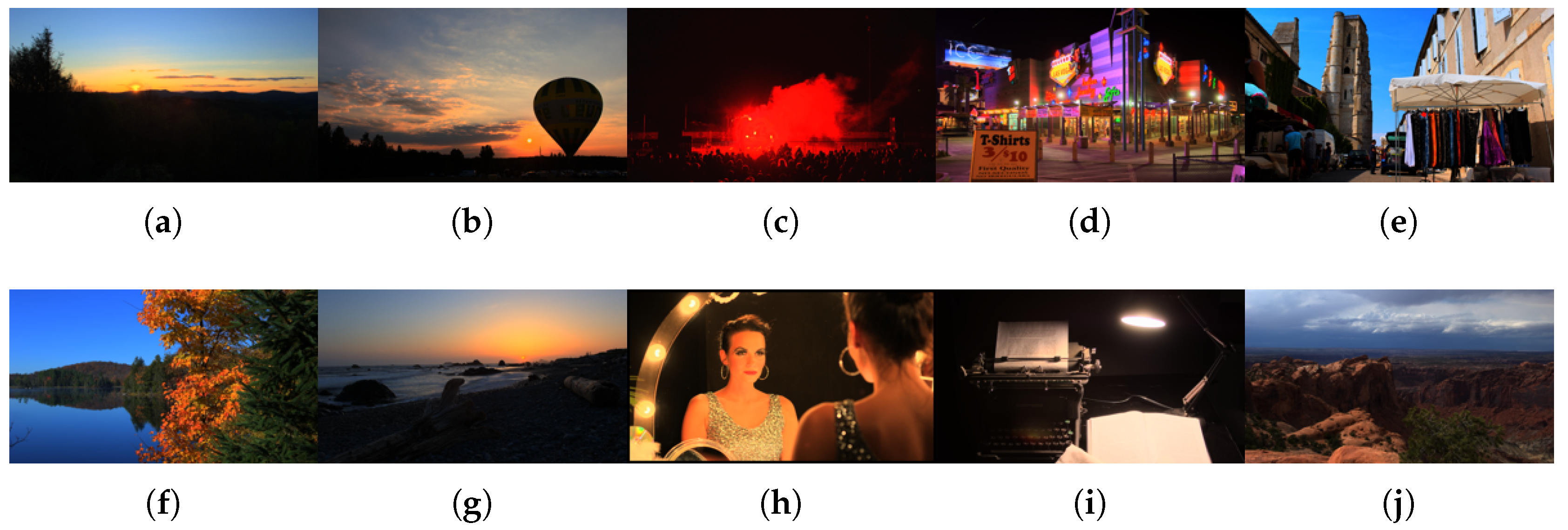
Figure A2.
Tone-mapped version (Reinhard et al. TMO [54]) of Zerman et al. reference images. From left to right and from top to bottom: (a) AirBellowsGap (b) Balloon (c) FireEater (d) LasVegasStore (e) Market3 (f) MasonLake(1) (g) RedwoodSunset (h) Showgirl (i) Typewriter (j) UpheavalDome.
Figure A2.
Tone-mapped version (Reinhard et al. TMO [54]) of Zerman et al. reference images. From left to right and from top to bottom: (a) AirBellowsGap (b) Balloon (c) FireEater (d) LasVegasStore (e) Market3 (f) MasonLake(1) (g) RedwoodSunset (h) Showgirl (i) Typewriter (j) UpheavalDome.

Appendix A.3. Korshunov et al.
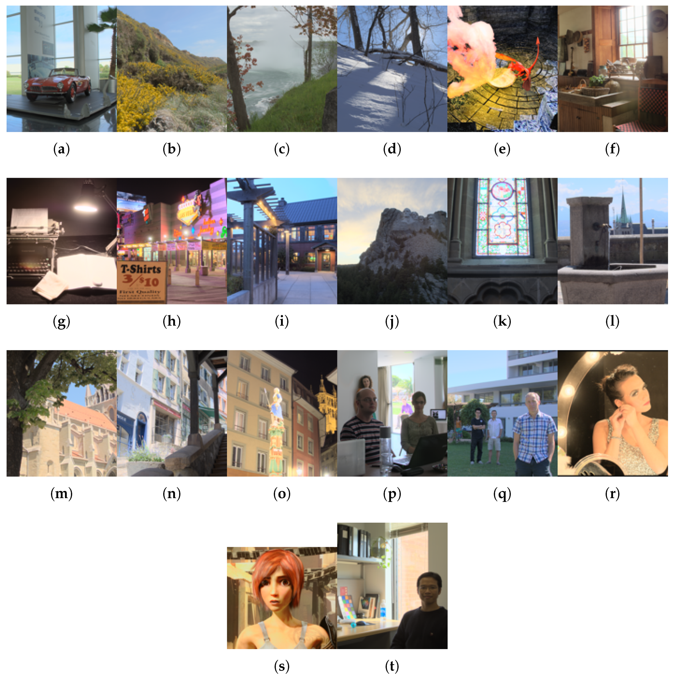
Figure A3.
Tone-mapped version (Reinhard et al. TMO [54]) of Korshunov et al. reference images. From left to right and from top to bottom: (a) 507 (b) BloomingGorse2 (c) CanadianFalls (d) DevilsBathtub (e) dragon_ 3 (f) HancockKitchenInside (g) LabTypewriter (h) LasVegasStore (i) McKeesPub (j) MtRushmore2 (k) set18 (l)set22 (m) set23 (n) set24 (o) set31 (p) set33 (q) set70 (r) showgirl (s) sintel_ 2 (t) WillyDesk.

Appendix A.4. HDdtb
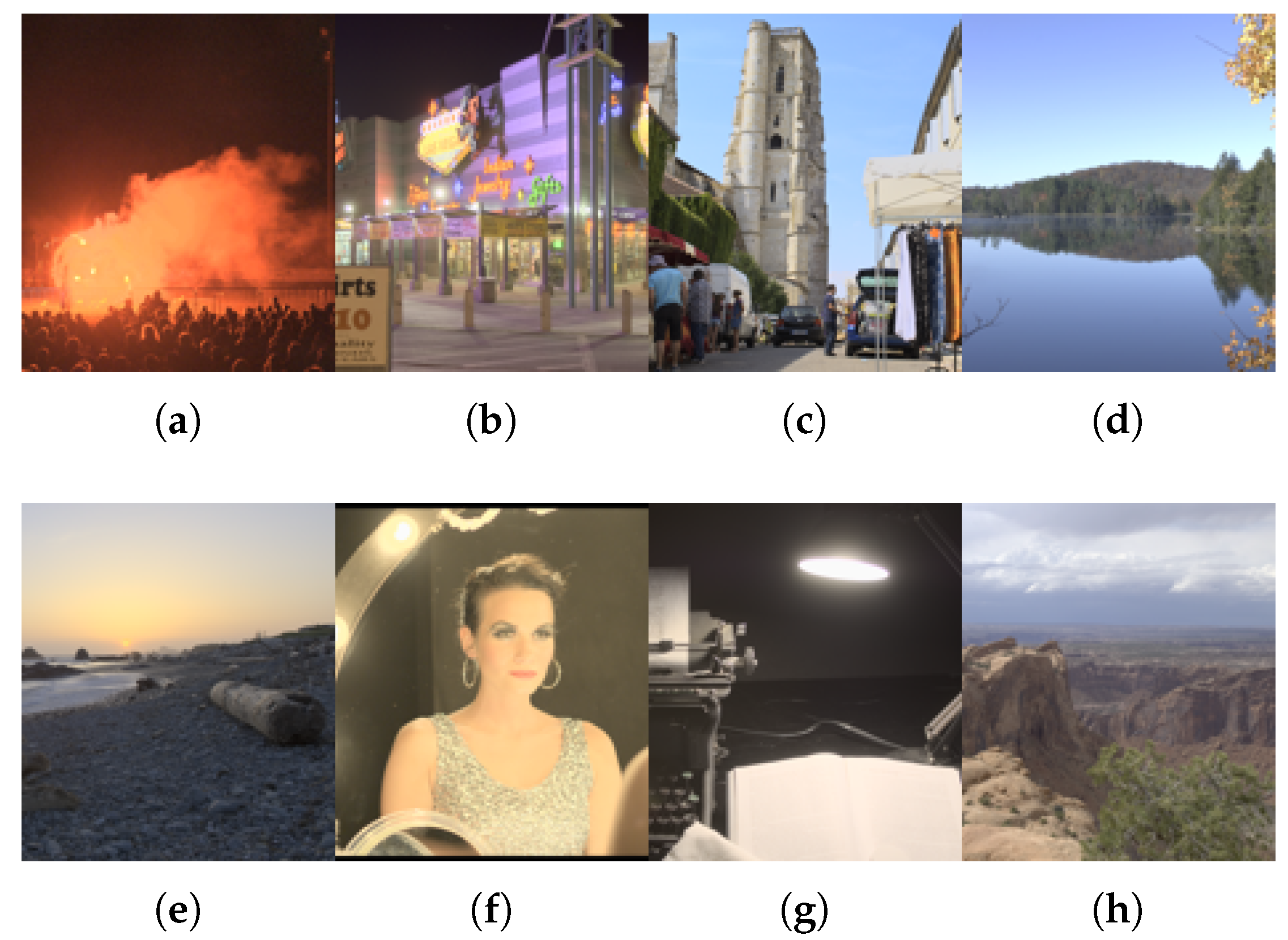
Figure A4.
Tone-mapped version (Reinhard et al. TMO [54]) of the HDdtb reference images. From left to right and from top to bottom: (a) FireEater (b) LasVegasStore (c) Market3 (d) MasonLake(1) (e) RedwoodSunset (f) Showgirl (g) Typewriter (h) UpheavalDome.
Figure A4.
Tone-mapped version (Reinhard et al. TMO [54]) of the HDdtb reference images. From left to right and from top to bottom: (a) FireEater (b) LasVegasStore (c) Market3 (d) MasonLake(1) (e) RedwoodSunset (f) Showgirl (g) Typewriter (h) UpheavalDome.

Appendix A.5. 4Kdtb
Figure A5.
Tone-mapped version (Reinhard et al. TMO [54]) of the 4Kdtb reference images. From left to right and from top to bottom: (a) Bike_ 20s (b) Bike_ 30s (c) Bike_ 81s (d) Bike_ 110s (e) Regatta_ 11s (f) Regatta_ 24s (g) Regatta_ 80s (h) Regatta_ 95s.
Figure A5.
Tone-mapped version (Reinhard et al. TMO [54]) of the 4Kdtb reference images. From left to right and from top to bottom: (a) Bike_ 20s (b) Bike_ 30s (c) Bike_ 81s (d) Bike_ 110s (e) Regatta_ 11s (f) Regatta_ 24s (g) Regatta_ 80s (h) Regatta_ 95s.

Appendix B. Performance Indexes
In this appendix, we present the numerical value for the performance indexes presented in Section 3.2 of each quality metrics with each database. The metrics with the best performances in terms of SROCC and PCC is in red, the second is in blue and the third in green.

Table A1.
PCC of the different color-blind quality metrics on the considered databases.
| Quality Metric | 4Kdtb | HDdtb | Narwaria et al. | Korshunov et al. | Zerman et al. |
|---|---|---|---|---|---|
| 0.6964 | 0.8002 | 0.5831 | 0.8597 | 0.8188 | |
| 0.6724 | 0.7950 | 0.5562 | 0.8602 | 0.8042 | |
| 0.4711 | 0.7320 | 0.5344 | 0.8004 | 0.7023 | |
| 0.7231 | 0.7948 | 0.6036 | 0.8697 | 0.8546 | |
| 0.5431 | 0.6899 | 0.5533 | 0.7999 | 0.7002 | |
| 0.1890 | 0.6416 | 0.4627 | 0.7017 | 0.5612 | |
| 0.2674 | 0.6755 | 0.4996 | 0.7635 | 0.6428 | |
| 0.6962 | 0.8520 | 0.7567 | 0.9265 | 0.8262 | |
| 0.6966 | 0.8448 | 0.7805 | 0.9243 | 0.8010 | |
| 0.6025 | 0.7677 | 0.7247 | 0.9021 | 0.6596 | |
| 0.6838 | 0.8366 | 0.7572 | 0.9296 | 0.8522 | |
| 0.6580 | 0.7851 | 0.7990 | 0.9174 | 0.6923 | |
| 0.2755 | 0.6174 | 0.6167 | 0.7786 | 0.4863 | |
| 0.3435 | 0.6729 | 0.6718 | 0.8423 | 0.5343 | |
| 0.8479 | 0.8881 | 0.8756 | 0.9631 | 0.9324 | |
| 0.8451 | 0.8899 | 0.8448 | 0.9606 | 0.9253 | |
| 0.7792 | 0.8395 | 0.8680 | 0.9068 | 0.7633 | |
| 0.8382 | 0.8763 | 0.8846 | 0.9575 | 0.9410 | |
| 0.8337 | 0.8603 | 0.9157 | 0.9694 | 0.8013 | |
| 0.4377 | 0.6422 | 0.6316 | 0.8619 | 0.6258 | |
| 0.5409 | 0.7062 | 0.7091 | 0.9126 | 0.6443 | |
| 0.9000 | 0.8443 | 0.8773 | 0.9568 | 0.8988 | |
| 0.8950 | 0.8476 | 0.8726 | 0.9540 | 0.9120 | |
| 0.8416 | 0.8923 | 0.8195 | 0.9733 | 0.9133 | |
| 0.8992 | 0.8234 | 0.8654 | 0.9471 | 0.8883 | |
| 0.8829 | 0.9187 | 0.8466 | 0.9724 | 0.9059 | |
| 0.5817 | 0.7372 | 0.6546 | 0.9015 | 0.7402 | |
| 0.7054 | 0.8066 | 0.7445 | 0.9215 | 0.8148 | |
| 0.8169 | 0.7963 | 0.6090 | 0.9210 | 0.9120 | |
| 0.8200 | 0.8023 | 0.5942 | 0.9218 | 0.9110 | |
| 0.6674 | 0.7088 | 0.5874 | 0.9252 | 0.8588 | |
| 0.8187 | 0.7762 | 0.6269 | 0.9297 | 0.9226 | |
| 0.7316 | 0.6624 | 0.5807 | 0.9120 | 0.8310 | |
| 0.3016 | 0.6320 | 0.4517 | 0.8102 | 0.6716 | |
| 0.4214 | 0.6540 | 0.5009 | 0.8972 | 0.7915 | |
| 0.8244 | 0.7873 | 0.7625 | 0.9364 | 0.8893 | |
| 0.8129 | 0.7693 | 0.7647 | 0.9360 | 0.8850 | |
| 0.6676 | 0.7545 | 0.7221 | 0.9368 | 0.8516 | |
| 0.8410 | 0.8140 | 0.7904 | 0.9310 | 0.9230 | |
| 0.7298 | 0.7592 | 0.7427 | 0.9261 | 0.8322 | |
| 0.3022 | 0.6750 | 0.5069 | 0.8574 | 0.6794 | |
| 0.4216 | 0.7203 | 0.6406 | 0.8942 | 0.7933 | |
| 0.8605 | 0.8715 | 0.9130 | 0.9518 | 0.9385 | |
| 0.7714 | 0.8676 | 0.9061 | 0.9612 | 0.9304 | |
| 0.8722 | 0.7645 | 0.7571 | 0.9215 | 0.8919 |
Table A2.
PCC of the different color quality metrics on the considered databases.
| Quality Metric | 4Kdtb | HDdtb | Narwaria et al. | Korshunov et al. | Zerman et al. |
|---|---|---|---|---|---|
| 0.4582 | 0.2502 | 0.6407 | 0.7629 | 0.6012 | |
| 0.2280 | 0.2559 | 0.6106 | 0.7024 | 0.5133 | |
| 0.6783 | 0.2548 | 0.6277 | 0.8065 | 0.7508 | |
| 0.4058 | 0.2952 | 0.6436 | 0.5536 | 0.5392 | |
| 0.2184 | 0.3438 | 0.3375 | 0.5993 | 0.3564 | |
| 0.2336 | 0.3083 | 0.3220 | 0.6873 | 0.4287 | |
| 0.7513 | 0.1135 | 0.6686 | 0.7334 | 0.7464 | |
| 0.4662 | 0.1027 | 0.5763 | 0.7470 | 0.6723 | |
| 0.7885 | 0.1355 | 0.5541 | 0.7639 | 0.7655 | |
| 0.6103 | 0.1331 | 0.5520 | 0.7556 | 0.6980 | |
| 0.2748 | 0.2698 | 0.2761 | 0.7152 | 0.4372 | |
| 0.3093 | 0.2047 | 0.2527 | 0.7250 | 0.6325 | |
| 0.5246 | 0.7050 | 0.7485 | 0.8845 | 0.7126 | |
| 0.3120 | 0.6618 | 0.7886 | 0.8664 | 0.5507 | |
| 0.7376 | 0.7764 | 0.7505 | 0.9176 | 0.8275 | |
| 0.5108 | 0.6842 | 0.8153 | 0.8914 | 0.6253 | |
| 0.2596 | 0.6020 | 0.6292 | 0.7713 | 0.4811 | |
| 0.2851 | 0.6187 | 0.7471 | 0.8354 | 0.5185 | |
| 0.7991 | 0.5193 | 0.7784 | 0.8929 | 0.7762 | |
| 0.5440 | 0.4249 | 0.6696 | 0.8828 | 0.6644 | |
| 0.7699 | 0.5137 | 0.7354 | 0.9152 | 0.8372 | |
| 0.6812 | 0.4872 | 0.6180 | 0.9197 | 0.7025 | |
| 0.2174 | 0.3671 | 0.4213 | 0.7590 | 0.4856 | |
| 0.3065 | 0.4367 | 0.5317 | 0.8788 | 0.5649 | |
| 0.8473 | 0.8598 | 0.8680 | 0.9360 | 0.9131 | |
| 0.6891 | 0.8654 | 0.8343 | 0.9633 | 0.9055 | |
| 0.9080 | 0.8086 | 0.8687 | 0.9453 | 0.8894 | |
| 0.8355 | 0.9162 | 0.8566 | 0.9717 | 0.9092 | |
| 0.5848 | 0.7337 | 0.6609 | 0.9029 | 0.7415 | |
| 0.6783 | 0.7923 | 0.7656 | 0.9541 | 0.8162 | |
| 0.5602 | 0.4489 | 0.6744 | 0.7533 | 0.7229 | |
| 0.3573 | 0.3986 | 0.6701 | 0.7275 | 0.6457 | |
| 0.7540 | 0.6467 | 0.7899 | 0.8608 | 0.8195 | |
| 0.4963 | 0.4749 | 0.7319 | 0.8196 | 0.7213 | |
| 0.2057 | 0.5711 | 0.5884 | 0.8328 | 0.6327 | |
| 0.3580 | 0.6153 | 0.7185 | 0.8942 | 0.7432 |
Table A3.
SROCC of the different color-blind quality metrics on the considered databases.
| Quality Metric | 4Kdtb | HDdtb | Narwaria et al. | Korshunov et al. | Zerman et al. |
|---|---|---|---|---|---|
| 0.7261 | 0.7802 | 0.5331 | 0.8597 | 0.8266 | |
| 0.6596 | 0.7751 | 0.4975 | 0.8602 | 0.8147 | |
| 0.4673 | 0.7587 | 0.4197 | 0.8078 | 0.7086 | |
| 0.7419 | 0.7745 | 0.5736 | 0.8742 | 0.8508 | |
| 0.5531 | 0.6933 | 0.4634 | 0.8102 | 0.7001 | |
| 0.2131 | 0.6311 | 0.4601 | 0.7216 | 0.5682 | |
| 0.2519 | 0.6687 | 0.4157 | 0.7756 | 0.6493 | |
| 0.7066 | 0.8430 | 0.7240 | 0.9280 | 0.8316 | |
| 0.6977 | 0.8355 | 0.7494 | 0.9253 | 0.8090 | |
| 0.6054 | 0.7904 | 0.7247 | 0.9085 | 0.6851 | |
| 0.6752 | 0.8245 | 0.7231 | 0.9307 | 0.8618 | |
| 0.6492 | 0.7813 | 0.7721 | 0.9181 | 0.7073 | |
| 0.1965 | 0.6488 | 0.5938 | 0.7746 | 0.5065 | |
| 0.3027 | 0.6926 | 0.6376 | 0.8421 | 0.5563 | |
| 0.8517 | 0.8640 | 0.8656 | 0.9583 | 0.9165 | |
| 0.8448 | 0.8708 | 0.8200 | 0.9567 | 0.9143 | |
| 0.7684 | 0.8505 | 0.8528 | 0.9600 | 0.7791 | |
| 0.8447 | 0.8464 | 0.8714 | 0.9529 | 0.9260 | |
| 0.8306 | 0.8557 | 0.9088 | 0.9648 | 0.8109 | |
| 0.4334 | 0.6864 | 0.6092 | 0.8646 | 0.6104 | |
| 0.5202 | 0.7296 | 0.6846 | 0.9124 | 0.6499 | |
| 0.9054 | 0.8149 | 0.8773 | 0.9553 | 0.8912 | |
| 0.8994 | 0.8239 | 0.8726 | 0.9553 | 0.9091 | |
| 0.8420 | 0.8799 | 0.8195 | 0.9692 | 0.9087 | |
| 0.9049 | 0.8099 | 0.8654 | 0.9477 | 0.8863 | |
| 0.8849 | 0.9069 | 0.8466 | 0.9663 | 0.9031 | |
| 0.5732 | 0.7546 | 0.6316 | 0.8986 | 0.7393 | |
| 0.7052 | 0.8153 | 0.7264 | 0.9415 | 0.8190 | |
| 0.8401 | 0.7803 | 0.5624 | 0.9331 | 0.9035 | |
| 0.8110 | 0.7856 | 0.5455 | 0.9333 | 0.9028 | |
| 0.6607 | 0.7508 | 0.4557 | 0.9311 | 0.8486 | |
| 0.8452 | 0.7554 | 0.5846 | 0.9308 | 0.9066 | |
| 0.7315 | 0.6501 | 0.4963 | 0.9230 | 0.8286 | |
| 0.2891 | 0.6314 | 0.4392 | 0.8449 | 0.6793 | |
| 0.3922 | 0.6670 | 0.4157 | 0.9102 | 0.7954 | |
| 0.8403 | 0.8218 | 0.7634 | 0.9369 | 0.9041 | |
| 0.8114 | 0.8167 | 0.7458 | 0.9365 | 0.9034 | |
| 0.6607 | 0.7984 | 0.6907 | 0.9384 | 0.8493 | |
| 0.8455 | 0.8011 | 0.7696 | 0.9343 | 0.9076 | |
| 0.7287 | 0.7664 | 0.7094 | 0.9339 | 0.8294 | |
| 0.2895 | 0.6773 | 0.4979 | 0.8692 | 0.6831 | |
| 0.3926 | 0.7160 | 0.6246 | 0.9236 | 0.7954 | |
| 0.8678 | 0.8685 | 0.8906 | 0.9516 | 0.9289 | |
| 0.7735 | 0.8330 | 0.8995 | 0.9572 | 0.9170 | |
| 0.8658 | 0.7464 | 0.7704 | 0.9322 | 0.8863 |
Table A4.
SROCC of the different color quality metrics on the considered databases.
| Quality Metric | 4Kdtb | HDdtb | Narwaria et al. | Korshunov et al. | Zerman et al. |
|---|---|---|---|---|---|
| 0.4807 | 0.2578 | 0.6490 | 0.7523 | 0.6394 | |
| 0.2123 | 0.2418 | 0.6179 | 0.6945 | 0.5259 | |
| 0.6846 | 0.3401 | 0.6218 | 0.8448 | 0.7599 | |
| 0.3008 | 0.2994 | 0.6339 | 0.6694 | 0.5602 | |
| 0.0739 | 0.3949 | 0.3896 | 0.6850 | 0.4436 | |
| 0.1549 | 0.3992 | 0.4377 | 0.7297 | 0.4999 | |
| 0.7827 | 0.2784 | 0.7181 | 0.8508 | 0.7559 | |
| 0.4898 | 0.2585 | 0.6207 | 0.8524 | 0.6851 | |
| 0.7911 | 0.2606 | 0.6195 | 0.8635 | 0.7892 | |
| 0.6396 | 0.2804 | 0.5855 | 0.8771 | 0.7283 | |
| 0.1706 | 0.3651 | 0.3911 | 0.8130 | 0.5665 | |
| 0.2392 | 0.3485 | 0.3927 | 0.8674 | 0.6365 | |
| 0.5184 | 0.7085 | 0.7212 | 0.8873 | 0.7535 | |
| 0.2991 | 0.6641 | 0.7643 | 0.8943 | 0.6047 | |
| 0.7437 | 0.7748 | 0.7273 | 0.9174 | 0.8545 | |
| 0.5059 | 0.7134 | 0.7926 | 0.8943 | 0.6740 | |
| 0.1785 | 0.6325 | 0.6064 | 0.7670 | 0.5065 | |
| 0.2259 | 0.6393 | 0.7044 | 0.8392 | 0.5443 | |
| 0.7972 | 0.4065 | 0.7605 | 0.8981 | 0.7834 | |
| 0.5369 | 0.3257 | 0.6322 | 0.8857 | 0.6813 | |
| 0.7712 | 0.4696 | 0.7212 | 0.9173 | 0.8464 | |
| 0.6730 | 0.4242 | 0.6181 | 0.9197 | 0.7037 | |
| 0.1717 | 0.3592 | 0.3054 | 0.7713 | 0.4995 | |
| 0.2657 | 0.4307 | 0.3830 | 0.8805 | 0.5805 | |
| 0.8510 | 0.8531 | 0.8548 | 0.9332 | 0.9068 | |
| 0.6835 | 0.8560 | 0.8196 | 0.9575 | 0.9025 | |
| 0.9127 | 0.7892 | 0.8585 | 0.9449 | 0.8852 | |
| 0.8371 | 0.9065 | 0.8485 | 0.9657 | 0.9046 | |
| 0.5784 | 0.7483 | 0.6376 | 0.8999 | 0.7413 | |
| 0.6799 | 0.7966 | 0.7512 | 0.9500 | 0.8196 | |
| 0.5533 | 0.4042 | 0.6592 | 0.7664 | 0.7337 | |
| 0.3534 | 0.3394 | 0.7138 | 0.7446 | 0.6589 | |
| 0.7618 | 0.6373 | 0.7585 | 0.8638 | 0.8418 | |
| 0.4893 | 0.4293 | 0.7065 | 0.8287 | 0.7301 | |
| 0.2282 | 0.5431 | 0.5565 | 0.8455 | 0.6315 | |
| 0.3443 | 0.5669 | 0.6851 | 0.9025 | 0.7486 |
Table A5.
OR of the different color-blind quality metrics on the considered databases.
| Quality Metric | 4Kdtb | HDdtb | Narwaria et al. | Korshunov et al. | Zerman et al. |
|---|---|---|---|---|---|
| 0.6354 | 0.5729 | 0.7714 | 0.5833 | 0.6400 | |
| 0.6458 | 0.5833 | 0.8857 | 0.6042 | 0.6800 | |
| 0.6563 | 0.5625 | 0.7714 | 0.6667 | 0.7000 | |
| 0.5938 | 0.5833 | 0.7786 | 0.5958 | 0.6100 | |
| 0.6563 | 0.6042 | 0.8143 | 0.6500 | 0.7400 | |
| 0.6875 | 0.6354 | 0.8429 | 0.8125 | 0.7700 | |
| 0.6979 | 0.6042 | 0.7714 | 0.7583 | 0.7300 | |
| 0.6354 | 0.4792 | 0.7786 | 0.4792 | 0.6500 | |
| 0.5938 | 0.4792 | 0.7857 | 0.4792 | 0.6500 | |
| 0.6458 | 0.4896 | 0.7571 | 0.5875 | 0.7100 | |
| 0.5833 | 0.5417 | 0.7929 | 0.4875 | 0.6700 | |
| 0.6771 | 0.5000 | 0.7500 | 0.5542 | 0.6900 | |
| 0.7083 | 0.6562 | 0.8071 | 0.7333 | 0.8700 | |
| 0.6979 | 0.5625 | 0.8286 | 0.7000 | 0.8000 | |
| 0.4063 | 0.5104 | 0.6786 | 0.3667 | 0.5000 | |
| 0.4375 | 0.4792 | 0.7357 | 0.3915 | 0.5400 | |
| 0.5000 | 0.4792 | 0.7143 | 0.3708 | 0.7000 | |
| 0.4479 | 0.5521 | 0.6500 | 0.3958 | 0.4600 | |
| 0.4271 | 0.5729 | 0.6857 | 0.3500 | 0.6900 | |
| 0.6875 | 0.6250 | 0.8143 | 0.6333 | 0.8100 | |
| 0.6667 | 0.5625 | 0.7929 | 0.5667 | 0.7900 | |
| 0.3545 | 0.5000 | 0.6143 | 0.4167 | 0.5000 | |
| 0.3750 | 0.5208 | 0.6714 | 0.4500 | 0.4400 | |
| 0.4479 | 0.5313 | 0.6357 | 0.3333 | 0.5300 | |
| 0.3229 | 0.5000 | 0.6714 | 0.4667 | 0.5200 | |
| 0.4167 | 0.5104 | 0.6500 | 0.3250 | 0.5900 | |
| 0.6562 | 0.5938 | 0.7714 | 0.5625 | 0.7800 | |
| 0.5833 | 0.5625 | 0.6786 | 0.4667 | 0.6900 | |
| 0.4896 | 0.6563 | 0.7500 | 0.5875 | 0.6600 | |
| 0.4583 | 0.6250 | 0.7643 | 0.5875 | 0.6400 | |
| 0.5938 | 0.6458 | 0.8071 | 0.5333 | 0.6600 | |
| 0.4583 | 0.7083 | 0.7857 | 0.5125 | 0.5900 | |
| 0.5521 | 0.6875 | 0.7571 | 0.5750 | 0.6700 | |
| 0.6979 | 0.6354 | 0.8500 | 0.7042 | 0.7600 | |
| 0.6667 | 0.6771 | 0.8214 | 0.5875 | 0.7200 | |
| 0.4167 | 0.7188 | 0.8071 | 0.5125 | 0.6200 | |
| 0.4792 | 0.7083 | 0.7786 | 0.5292 | 0.6100 | |
| 0.5833 | 0.6667 | 0.7571 | 0.4625 | 0.6500 | |
| 0.4271 | 0.6667 | 0.7643 | 0.5375 | 0.5700 | |
| 0.6032 | 0.5938 | 0.7643 | 0.5292 | 0.6800 | |
| 0.6979 | 0.6146 | 0.8429 | 0.6833 | 0.7500 | |
| 0.6667 | 0.5833 | 0.7857 | 0.6333 | 0.7100 | |
| 0.3545 | 0.4576 | 0.6250 | 0.3708 | 0.4400 | |
| 0.5313 | 0.5616 | 0.9061 | 0.392 | 0.5300 | |
| 0.4063 | 0.5938 | 0.7571 | 0.5833 | 0.5500 |
Table A6.
OR of the different color quality metrics on the considered databases.
| Quality Metric | 4Kdtb | HDdtb | Narwaria et al. | Korshunov et al. | Zerman et al. |
|---|---|---|---|---|---|
| 0.7083 | 0.7604 | 0.7714 | 0.7167 | 0.8100 | |
| 0.7083 | 0.7604 | 0.7929 | 0.7500 | 0.8000 | |
| 0.6354 | 0.7708 | 0.8357 | 0.7833 | 0.6900 | |
| 0.6458 | 0.7604 | 0.8429 | 0.8542 | 0.8000 | |
| 0.6562 | 0.7500 | 0.8643 | 0.8333 | 0.8500 | |
| 0.6875 | 0.8714 | 0.8429 | 0.7756 | 0.8700 | |
| 0.5417 | 0.7813 | 0.8214 | 0.8083 | 0.7100 | |
| 0.6667 | 0.7708 | 0.8143 | 0.8000 | 0.7600 | |
| 0.4792 | 0.7813 | 0.8214 | 0.8583 | 0.6800 | |
| 0.6563 | 0.7813 | 0.8429 | 0.7792 | 0.7400 | |
| 0.6875 | 0.7500 | 0.8714 | 0.8000 | 0.8600 | |
| 0.6771 | 0.7396 | 0.8500 | 0.7792 | 0.7500 | |
| 0.6979 | 0.5625 | 0.7929 | 0.6208 | 0.6900 | |
| 0.7083 | 0.6458 | 0.7429 | 0.8458 | 0.8000 | |
| 0.5729 | 0.5729 | 0.8429 | 0.5292 | 0.6400 | |
| 0.6979 | 0.5625 | 0.6929 | 0.6167 | 0.7300 | |
| 0.7188 | 0.6667 | 0.8000 | 0.7292 | 0.8700 | |
| 0.7188 | 0.6667 | 0.7643 | 0.6542 | 0.8000 | |
| 0.5417 | 0.6979 | 0.8071 | 0.6458 | 0.6700 | |
| 0.6771 | 0.7604 | 0.7500 | 0.6667 | 0.7700 | |
| 0.5000 | 0.8021 | 0.8143 | 0.6458 | 0.6900 | |
| 0.6667 | 0.7396 | 0.8286 | 0.6125 | 0.7600 | |
| 0.6979 | 0.7708 | 0.7929 | 0.7167 | 0.6900 | |
| 0.7083 | 0.7708 | 0.8000 | 0.6167 | 0.7600 | |
| 0.4375 | 0.5625 | 0.5928 | 0.5083 | 0.5600 | |
| 0.6563 | 0.5000 | 0.6357 | 0.3625 | 0.6200 | |
| 0.2917 | 0.5938 | 0.5857 | 0.4833 | 0.5500 | |
| 0.4375 | 0.4271 | 0.6714 | 0.3208 | 0.5500 | |
| 0.6458 | 0.5729 | 0.7786 | 0.5667 | 0.7700 | |
| 0.6562 | 0.5729 | 0.6786 | 0.3625 | 0.6900 | |
| 0.6354 | 0.7500 | 0.7571 | 0.7500 | 0.7300 | |
| 0.6458 | 0.7813 | 0.7643 | 0.7417 | 0.7400 | |
| 0.5104 | 0.7188 | 0.7500 | 0.6375 | 0.7600 | |
| 0.6458 | 0.7396 | 0.7357 | 0.6542 | 0.7300 | |
| 0.6667 | 0.6771 | 0.7571 | 0.6875 | 0.7500 | |
| 0.6771 | 0.6979 | 0.7000 | 0.5958 | 0.7500 |
Table A7.
RMSE of the different color-blind quality metrics on the considered databases.
| Quality Metric | 4Kdtb | HDdtb | Narwaria et al. | Korshunov et al. | Zerman et al. |
|---|---|---|---|---|---|
| 15.87 | 17.09 | 20.43 | 16.00 | 17.08 | |
| 16.44 | 17.45 | 24.95 | 15.97 | 17.66 | |
| 19.52 | 19.79 | 21.27 | 18.77 | 21.14 | |
| 15.32 | 16.81 | 20.05 | 15.46 | 15.49 | |
| 18.66 | 20.02 | 20.92 | 18.79 | 21.21 | |
| 21.80 | 21.24 | 22.36 | 22.31 | 24.58 | |
| 21.38 | 20.42 | 21.79 | 20.23 | 22.75 | |
| 15.92 | 14.48 | 16.44 | 11.75 | 16.69 | |
| 15.91 | 14.81 | 15.73 | 11.86 | 17.78 | |
| 17.70 | 17.08 | 16.12 | 13.52 | 22.41 | |
| 15.91 | 15.16 | 16.43 | 11.54 | 15.28 | |
| 16.70 | 17.14 | 15.13 | 12.46 | 21.20 | |
| 21.32 | 21.79 | 19.80 | 19.65 | 25.95 | |
| 20.89 | 20.49 | 18.63 | 16.88 | 25.11 | |
| 11.76 | 12.73 | 12.15 | 8.43 | 10.73 | |
| 11.86 | 12.62 | 13.46 | 8.71 | 11.26 | |
| 13.62 | 15.03 | 12.49 | 8.12 | 19.18 | |
| 12.10 | 13.33 | 11.73 | 9.04 | 10.53 | |
| 12.25 | 14.11 | 10.11 | 7.69 | 17.88 | |
| 19.95 | 21.23 | 19.65 | 15.88 | 23.17 | |
| 18.66 | 19.61 | 17.74 | 12.81 | 22.71 | |
| 9.67 | 14.84 | 12.07 | 9.11 | 13.02 | |
| 9.89 | 14.70 | 12.29 | 9.39 | 12.18 | |
| 11.98 | 12.50 | 14.41 | 7.19 | 12.09 | |
| 9.70 | 15.70 | 12.60 | 10.05 | 13.64 | |
| 10.42 | 10.94 | 13.39 | 7.31 | 12.58 | |
| 18.04 | 18.71 | 19.01 | 13.55 | 19.97 | |
| 15.72 | 16.37 | 16.79 | 11.60 | 17.22 | |
| 12.80 | 16.75 | 19.95 | 15.39 | 12.19 | |
| 12.70 | 16.53 | 20.23 | 12.14 | 14.20 | |
| 16.52 | 19.54 | 20.36 | 11.88 | 15.21 | |
| 12.74 | 17.45 | 19.60 | 11.54 | 11.45 | |
| 15.12 | 20.75 | 20.48 | 12.85 | 16.52 | |
| 21.15 | 21.46 | 22.44 | 18.36 | 22.01 | |
| 20.12 | 20.95 | 21.77 | 13.83 | 18.15 | |
| 12.55 | 17.07 | 16.28 | 10.99 | 13.60 | |
| 12.92 | 17.70 | 16.21 | 11.10 | 14.10 | |
| 16.51 | 18.20 | 17.40 | 10.96 | 15.62 | |
| 12.00 | 16.09 | 15.41 | 11.60 | 11.43 | |
| 15.16 | 18.11 | 16.84 | 11.82 | 16.47 | |
| 21.14 | 20.43 | 21.68 | 16.12 | 21.79 | |
| 20.11 | 19.21 | 19.31 | 14.04 | 18.08 | |
| 11.3 | 12.55 | 11.27 | 9.60 | 9.50 | |
| 14.11 | 14.72 | 10.64 | 8.57 | 10.88 | |
| 10.85 | 17.85 | 15.74 | 12.17 | 13.43 |
Table A8.
RMSE of the different color quality metrics on the considered databases.
| Quality Metric | 4Kdtb | HDdtb | Narwaria et al. | Korshunov et al. | Zerman et al. |
|---|---|---|---|---|---|
| 19.72 | 26.81 | 19.31 | 20.25 | 23.73 | |
| 21.60 | 26.77 | 19.92 | 22.29 | 25.49 | |
| 16.30 | 27.11 | 19.58 | 19.99 | 19.62 | |
| 20.28 | 26.46 | 19.25 | 26.08 | 25.01 | |
| 21.64 | 26.01 | 23.68 | 27.51 | 28.31 | |
| 21.57 | 26.36 | 23.82 | 22.77 | 26.83 | |
| 14.64 | 27.51 | 18.70 | 21.30 | 19.77 | |
| 19.67 | 27.68 | 20.56 | 20.82 | 21.99 | |
| 13.64 | 27.61 | 20.94 | 28.91 | 18.10 | |
| 17.58 | 27.44 | 21.45 | 20.53 | 20.35 | |
| 21.33 | 26.67 | 24.18 | 21.90 | 26.71 | |
| 21.09 | 27.11 | 24.34 | 21.59 | 23.00 | |
| 18.88 | 19.62 | 16.68 | 14.61 | 19.95 | |
| 21.07 | 20.74 | 15.46 | 15.92 | 24.30 | |
| 14.98 | 17.44 | 16.62 | 13.50 | 15.77 | |
| 19.07 | 20.18 | 14.56 | 14.20 | 22.63 | |
| 21.42 | 22.11 | 19.55 | 19.93 | 26.04 | |
| 21.26 | 21.76 | 16.72 | 17.22 | 25.40 | |
| 13.34 | 23.59 | 15.79 | 14.10 | 18.72 | |
| 18.61 | 25.05 | 18.68 | 14.71 | 22.20 | |
| 14.15 | 23.74 | 17.04 | 12.62 | 16.24 | |
| 16.24 | 24.16 | 20.41 | 16.47 | 21.14 | |
| 21.65 | 25.76 | 22.81 | 20.39 | 26.21 | |
| 21.11 | 24.91 | 21.30 | 14.94 | 24.51 | |
| 11.78 | 14.14 | 12.80 | 11.02 | 12.11 | |
| 16.07 | 13.88 | 13.87 | 8.41 | 12.0 | |
| 9.29 | 16.29 | 12.46 | 10.22 | 13.57 | |
| 12.19 | 11.09 | 12.98 | 7.40 | 12.36 | |
| 17.99 | 18.82 | 18.88 | 13.47 | 19.93 | |
| 16.30 | 16.90 | 16.18 | 9.38 | 17.17 | |
| 18.37 | 24.75 | 18.57 | 20.60 | 20.52 | |
| 20.72 | 25.40 | 18.70 | 21.49 | 22.68 | |
| 14.57 | 21.12 | 19.02 | 15.94 | 17.03 | |
| 19.26 | 24.37 | 17.14 | 17.94 | 20.57 | |
| 21.71 | 22.75 | 20.34 | 17.34 | 23.00 | |
| 20.71 | 21.83 | 17.49 | 14.02 | 19.87 |
Appendix C. Metrics Sensitivity on the Chrominance Artifacts with Our Proposed Database 4Kdtb
This appendix is an extension of the Section 5.2 where the impacts of the chrominance artifacts on quality metrics performances is studied. For each reference image of the database 4Kdtb, the subjective and objective scores for each distorted image are shown in function of the HEVC Qp. The objective scores are displayed after applying the logistic regression presented in Section 4.
The images compressed with the chroma Qp offset algorithm (cf. Section 3.1.2) are represented with a red line. The images compressed without the chroma Qp offset and 10 bits quantization on the chrominance with a green line. The images compressed without the chroma Qp offset algorithm and a 10 bits quantization are represented with a blue line.
Figure A6.
Subjective and objective scores for the image Bike_20s.

Figure A7.
Subjective and objective scores for the image Bike_30s.

Figure A8.
Subjective and objective scores for the image Bike_81s.

Figure A9.
Subjective and objective scores for the image Bike_110s.

Figure A10.
Subjective and objective scores for the image Regatta_11s

Figure A11.
Subjective and objective scores for the image Regatta_24s.

Figure A12.
Subjective and objective scores for the image Regatta_80s.

Figure A13.
Subjective and objective scores for the image Regatta_95s.

References
- Parameter Values for the HDTV Standard for Production and International Program Exchange; Rec BT.709-6, ITU-R; International Telecommunication Union (ITU): Geneva, Switzerland, 2015.
- Reference Electro-Optical Transfer Function for Flat Panel Displays Used in HDTV Studio Production; Rec BT.1886-0, ITU-R; International Telecommunication Union (ITU): Geneva, Switzerland, 2015.
- High Dynamic Range Electro-Optical Transfer Function of Mastering Reference Displays; Standard ST.2084; Society of Motion Picture & Television Engineers (SMPTE): White Plains, NY, USA, 2014.
- Essential Parameter Values for the Extended Image Dynamic Range Television System for Programme Production; Standard STD-B67; Association of Radio Industries and Businesses (ARIB): Tokyo, Japan, 2015.
- Parameter Values for Ultra-High Definition Television Systems for Production and International Programme Exchange; Rec BT.2020-2, ITU-R; International Telecommunication Union (ITU): Geneva, Switzerland, 2016.
- Image Parameter Values for High Dynamic Range Television for Use in Production and International Programme Exchange; Rec BT.2100-1, ITU-R; International Telecommunication Union (ITU): Geneva, Switzerland, 2017.
- Aydın, T.O.; Mantiuk, R.; Seidel, H.P. Extending quality metrics to full luminance range images. Proc. SPIE 2008, 6806. [Google Scholar] [CrossRef]
- Wang, Z.; Bovik, A.C.; Sheikh, H.R.; Simoncelli, E.P. Image quality assessment: From error visibility to structural similarity. IEEE Trans. Image Process. 2004, 13, 600–612. [Google Scholar] [CrossRef] [PubMed]
- Sheikh, H.R.; Bovik, A.C. Image information and visual quality. In Proceedings of the 2004 IEEE International Conference on Acoustics, Speech, and Signal Processing, Montreal, QC, Canada, 17–21 May 2004; Volume 3, pp. iii–709. [Google Scholar] [CrossRef]
- Wang, Z.; Simoncelli, E.P.; Bovik, A.C. Multiscale structural similarity for image quality assessment. In Proceedings of the The Thrity-Seventh Asilomar Conference on Signals, Systems Computers, Pacific Grove, CA, USA, 9–12 November 2003; Volume 2, pp. 1398–1402. [Google Scholar] [CrossRef]
- Mantiuk, R.; Kim, K.J.; Rempel, A.G.; Heidrich, W. HDR-VDP-2: A Calibrated Visual Metric for Visibility and Quality Predictions in All Luminance Conditions. ACM Trans. Graph. 2011, 30, 40:1–40:14. [Google Scholar] [CrossRef]
- Narwaria, M.; Mantiuk, R.; Da Silva, M.P.; Le Callet, P. HDR-VDP-2.2: A calibrated method for objective quality prediction of high-dynamic range and standard images. J. Electron. Imaging 2015, 24, 010501. [Google Scholar] [CrossRef]
- Narwaria, M.; Da Silva, M.P.; Le Callet, P. HDR-VQM: An objective quality measure for high dynamic range video. Signal Process. Image Commun. 2015, 35, 46–60. [Google Scholar] [CrossRef] [Green Version]
- Hanhart, P.; Bernardo, M.V.; Pereira, M.; Pinheiro, A.M.G.; Ebrahimi, T. Benchmarking of objective quality metrics for HDR image quality assessment. EURASIP J. Image Video Process. 2015, 2015, 39. [Google Scholar] [CrossRef]
- Richter, T. On the standardization of the JPEG XT image compression. In Proceedings of the 2013 Picture Coding Symposium (PCS), San Jose, CA, USA, 8–11 December 2013; pp. 37–40. [Google Scholar] [CrossRef]
- Hanhart, P.; Řeřábek, M.; Ebrahimi, T. Towards high dynamic range extensions of HEVC: Subjective evaluation of potential coding technologies. Proc. SPIE 2015, 9599. [Google Scholar] [CrossRef]
- Hanhart, P.; Řeřábek, M.; Ebrahimi, T. Subjective and objective evaluation of HDR video coding technologies. In Proceedings of the International Conference on Quality of Multimedia Experience (QoMEX), Lisbon, Portugal, 6–8 June 2016; pp. 1–6. [Google Scholar]
- Vigier, T.; Krasula, L.; Milliat, A.; Perreira Da Silva, M.; Le Callet, P. Performance and robustness of HDR objective quality metrics in the context of recent compression scenarios. In Proceedings of the Digital Media Industry and Academic Forum, Santorini, Greece, 4–6 July 2016; pp. 59–64. [Google Scholar] [CrossRef]
- Zerman, E.; Valenzise, G.; Dufaux, F. An extensive performance evaluation of full-reference HDR image quality metrics. Qual. User Exp. 2017, 2, 5. [Google Scholar] [CrossRef]
- Fairchild, M.D.; Chen, P.H. Brightness, lightness, and specifying color in high-dynamic-range scenes and images. Proc. SPIE 2011, 7867. [Google Scholar] [CrossRef]
- Colorimetry—Part 4: CIE 1976 L*A*B* Colour Space; Standard CIE S014-4/E:2007; Commision Internationale de l’Eclairage: Vienna, Austria, 1976.
- Safdar, M.; Cui, G.; Kim, Y.J.; Luo, M.R. Perceptually uniform color space for image signals including high dynamic range and wide gamut. Opt. Express 2017, 25, 15131–15151. [Google Scholar] [CrossRef]
- Ebner, F.; Fairchild, M.D. Development and testing of a color space (IPT) with improved hue uniformity. In Proceedings of the Color and Imaging Conference, Scottsdale, AZ, USA, 17–20 November 1998; Society for Imaging Science and Technology: Springfield, VA, USA, 1998; Volume 1998, pp. 8–13. [Google Scholar]
- What Is ICtCp? White paper Version 7.2; Dolby: San Francisco, CA, USA, 2017.
- Pieri, E.; Pytlarz, J. Hitting the Mark—A New Color Difference Metric for HDR and WCG Imagery. SMPTE Motion Imaging J. 2018, 127, 18–25. [Google Scholar] [CrossRef]
- Zhang, X.; Wandell, B.A. A spatial extension of CIELAB for digital color-image reproduction. J. Soc. Inf. Disp. 1997, 5, 61–63. [Google Scholar] [CrossRef]
- Wang, Z.; Lu, L.; Bovik, A.C. Video quality assessment based on structural distortion measurement. Signal Process. Image Commun. 2004, 19, 121–132. [Google Scholar] [CrossRef] [Green Version]
- Hassan, M.A.; Bashraheel, M.S. Color-based structural similarity image quality assessment. In Proceedings of the 2017 8th International Conference on Information Technology (ICIT), Amman, Jordan, 17–18 May 2017; pp. 691–696. [Google Scholar] [CrossRef]
- Zhang, L.; Zhang, L.; Mou, X.; Zhang, D. FSIM: A Feature Similarity Index for Image Quality Assessment. IEEE Trans. Image Process. 2011, 20, 2378–2386. [Google Scholar] [CrossRef] [PubMed] [Green Version]
- Ponomarenko, N.; Silvestri, F.; Egiazarian, K.; Carli, M.; Astola, J.; Lukin, V. On between-coefficient contrast masking of DCT basis functions. In Proceedings of the Third International Workshop on Video Processing and Quality Metrics, Scottsdale, AZ, USA, 25–26 January 2007; Volume 4. [Google Scholar]
- Ponomarenko, N.; Ieremeiev, O.; Lukin, V.; Egiazarian, K.; Jin, L.; Astola, J.; Vozel, B.; Chehdi, K.; Carli, M.; Battisti, F.; et al. Color image database TID2013: Peculiarities and preliminary results. In Proceedings of the 2013 4th European Workshop on Visual Information Processing (EUVIP), Paris, France, 10–12 June 2013. [Google Scholar]
- Subjective Video Quality Assessment Methods for Multimedia Applications; Rec P.910, ITU-T; International Telecommunication Union (ITU): Geneva, Switzerland, 2008.
- Hasler, D.; Suesstrunk, S.E. Measuring colorfulness in natural images. Proc. SPIE 2003, 5007. [Google Scholar] [CrossRef]
- Narwaria, M.; Da Silva, M.P.; Le Callet, P.; Pepion, R. Tone mapping-based high-dynamic-range image compression: Study of optimization criterion and perceptual quality. Opt. Eng. 2013, 52, 102008. [Google Scholar] [CrossRef]
- Korshunov, P.; Hanhart, P.; Richter, T.; Artusi, A.; Mantiuk, R.; Ebrahimi, T. Subjective quality assessment database of HDR images compressed with JPEG XT. In Proceedings of the 2015 Seventh International Workshop on Quality of Multimedia Experience (QoMEX), Pylos-Nestoras, Greece, 26–29 May 2015; pp. 1–6. [Google Scholar] [CrossRef]
- Kuang, J.; Johnson, G.M.; Fairchild, M.D. iCAM06: A refined image appearance model for HDR image rendering. J. Vis. Commun. Image Represent. 2007, 18, 406–414. [Google Scholar] [CrossRef]
- Mantiuk, R.; Myszkowski, K.; Seidel, H.P. A Perceptual Framework for Contrast Processing of High Dynamic Range Images. ACM Trans. Appl. Percept. 2006, 3, 286–308. [Google Scholar] [CrossRef]
- Reinhard, E.; Stark, M.; Shirley, P.; Ferwerda, J. Photographic Tone Reproduction for Digital Images. In Proceedings of the 29th Annual Conference on Computer Graphics and Interactive Techniques (SIGGRAPH ’02 ), San Antonio, TX, USA, 23–26 July 2002; ACM: New York, NY, USA, 2002; pp. 267–276. [Google Scholar] [CrossRef]
- Valenzise, G.; De Simone, F.; Lauga, P.; Dufaux, F. Performance evaluation of objective quality metrics for HDR image compression. Proc. SPIE 2014, 9217. [Google Scholar] [CrossRef]
- Mai, Z.; Mansour, H.; Mantiuk, R.; Nasiopoulos, P.; Ward, R.; Heidrich, W. Optimizing a Tone Curve for Backward-Compatible High Dynamic Range Image and Video Compression. IEEE Trans. Image Process. 2011, 20, 1558–1571. [Google Scholar] [CrossRef]
- Specification for the Use of Video and Audio Coding in Broadcast and Broadband Applications; Technical Specification ETSI TS 101 154 v2.4.1; Digital Video Broadcasting (DVB): Sophia Antipolis, France, 2018.
- Operation Manuals: BVM-X300; Manual Version 2.2; Sony: Tokyo, Japan, 2017.
- Methodology for the Subjective Assessment of the Quality of Television Pictures; Rec BT.500-13, ITU-R; International Telecommunication Union (ITU): Geneva, Switzerland, 2012.
- Conversion and Coding Practices for HDR/WCG Y’CbCr 4:2:0 Video with PQ Transfer Characteristics; Rec H-Suppl.15, ITU-T; International Telecommunication Union (ITU): Geneva, Switzerland, 2017.
- Rousselot, M.; Auffret, E.; Ducloux, X.; Le Meur, O.; Cozot, R. Impacts of Viewing Conditions on HDR-VDP2. In Proceedings of the 2018 26th European Signal Processing Conference (EUSIPCO), Rome, Italy, 3–7 September 2018; pp. 1442–1446. [Google Scholar] [CrossRef]
- Lasserre, S.; LeLéannec, F.; Francois, E. Description of HDR Sequences Proposed by Technicolor; ISO/IEC JTC1/SC29/WG11 JCTVC-P0228]; IEEE: San Jose, CA, USA, 2013. [Google Scholar]
- Froehlich, J.; Grandinetti, S.; Eberhardt, B.; Walter, S.; Schilling, A.; Brendel, H. Creating cinematic wide gamut HDR-video for the evaluation of tone mapping operators and HDR-displays. Proc. SPIE 2014, 9023. [Google Scholar] [CrossRef]
- Fairchild, M.D. The HDR photographic survey. In Proceedings of the Color and Imaging Conference, Albuquerque, NM, USA, 5–9 November 2007; Society for Imaging Science and Technology: Springfield, VA, USA, 2007; Volume 2007, pp. 233–238. [Google Scholar]
- Methods, Metrics and Procedures for Statistical Evaluation, Qualification And Comparison of Objective Quality Prediction Models; Rec P.1401, ITU-T; International Telecommunication Union (ITU): Geneva, Switzerland, 2012.
- Ponomarenko, N.; Ieremeiev, O.; Lukin, V.; Egiazarian, K.; Carli, M. Modified image visual quality metrics for contrast change and mean shift accounting. In Proceedings of the 2011 11th International Conference, The Experience of Designing and Application of CAD Systems in Microelectronics (CADSM), Polyana-Svalyava, Ukraine, 23–25 February 2011. [Google Scholar]
- Daly, S.J. Visible differences predictor: An algorithm for the assessment of image fidelity. Proc. SPIE 1992, 1666. [Google Scholar] [CrossRef]
- Barten, P.G.J. Formula for the contrast sensitivity of the human eye. Proc. SPIE 2003, 5294. [Google Scholar] [CrossRef]
- Operational Practices in HDR Television Production; Rec BT.2408-0, ITU-R; International Telecommunication Union (ITU): Geneva, Switzerland, 2017.
- Reinhard, E.; Stark, M.; Shirley, P.; Ferwerda, J. Photographic tone reproduction for digital images. ACM Trans. Graph. (TOG) 2002, 21, 267–276. [Google Scholar] [CrossRef]
- Banterle, F.; Artusi, A.; Debattista, K.; Chalmers, A. Advanced High Dynamic Range Imaging: Theory and Practice, 2nd ed.; AK Peters (CRC Press): Natick, MA, USA, 2017. [Google Scholar]
Figure 1.
Diagram of the proposed method to adapt SDR metrics to HDR/WCG contents.

Figure 2.
Different perceptually uniform luminances as a function of the linear luminance: (a) for the range 0–1000 , (b) for the range 0–150 .
Figure 2.
Different perceptually uniform luminances as a function of the linear luminance: (a) for the range 0–1000 , (b) for the range 0–150 .

Figure 3.
Characteristics of the Narwaria et al. [34] images: (a) The dynamic range, (b) key, (c) spatial Information, (d) Colorfulness.
Figure 3.
Characteristics of the Narwaria et al. [34] images: (a) The dynamic range, (b) key, (c) spatial Information, (d) Colorfulness.

Figure 4.
Characteristics of the Korshunov et al. [35] images: (a) The dynamic range, (b) key, (c) spatial Information, (d) Colorfulness.
Figure 4.
Characteristics of the Korshunov et al. [35] images: (a) The dynamic range, (b) key, (c) spatial Information, (d) Colorfulness.

Figure 5.
Characteristics of the Zerman et al. [19] images: (a) The dynamic range, (b) key, (c) spatial Information, (d) Colorfulness.
Figure 5.
Characteristics of the Zerman et al. [19] images: (a) The dynamic range, (b) key, (c) spatial Information, (d) Colorfulness.

Figure 6.
Characteristics of the HDdtb images: (a) The dynamic range, (b) key, (c) spatial Information, (d) Colorfulness.
Figure 6.
Characteristics of the HDdtb images: (a) The dynamic range, (b) key, (c) spatial Information, (d) Colorfulness.

Figure 7.
Characteristics of the 4Kdtb images: ((a) The dynamic range, (b) key, (c) spatial Information, (d) Colorfulness.
Figure 7.
Characteristics of the 4Kdtb images: ((a) The dynamic range, (b) key, (c) spatial Information, (d) Colorfulness.

Figure 8.
SROCC performances for the 4Kdtb database for color-blind quality metrics (a) and for color quality metrics (b).
Figure 8.
SROCC performances for the 4Kdtb database for color-blind quality metrics (a) and for color quality metrics (b).

Figure 9.
SROCC performances for the Zerman et al. database for color-blind quality metrics (a) and for color quality metrics (b).
Figure 9.
SROCC performances for the Zerman et al. database for color-blind quality metrics (a) and for color quality metrics (b).

Figure 10.
SROCC performances for the HDdtb database for color-blind quality metrics (a) and for color quality metrics (b).
Figure 10.
SROCC performances for the HDdtb database for color-blind quality metrics (a) and for color quality metrics (b).

Figure 11.
SROCC performances for the Korshunov et al. database for color-blind quality metrics (a) and for color quality metrics (b).
Figure 11.
SROCC performances for the Korshunov et al. database for color-blind quality metrics (a) and for color quality metrics (b).

Figure 12.
SROCC performances for the Narwaria et al. database for color-blind quality metrics (a) and for color quality metrics (b).
Figure 12.
SROCC performances for the Narwaria et al. database for color-blind quality metrics (a) and for color quality metrics (b).

Figure 13.
SROCC of (a) , (b) , (c) in function of the diffuse white luminance.

Figure 14.
Subjective and objective scores for the image Regatta_24s and for 6 metrics based on the color space.
Figure 14.
Subjective and objective scores for the image Regatta_24s and for 6 metrics based on the color space.

Table 1.
Selected SDR quality metrics.
| Name | Color | Reference | Main Principle |
|---|---|---|---|
| PSNR | Ratio between the range of the signal and the mean square error | ||
| ✓ | Mean of the color difference metrics | ||
| ✓ | Zhang et al. [26] | Mean of the color difference metrics by considering the blurring effect of the HVS. Also known as S-CIELab | |
| SSIM | Wang et al. [8] | Metrics based on the comparison of three characteristics of the images: the luminance, the contrast and the structure | |
| SSIMc | ✓ | Wang et al. [27] | Linear combination of the SSIM applied on the three components Y, Cr and Cb of the images. |
| CSSIM | ✓ | Hassan et al. [28] | Combination of SSIM and |
| MS-SSIM | Wang et al. [10] | Multi-scale SSIM | |
| FSIM | Zhang et al. [29] | Comparison of the phase congruency and the gradient magnitude | |
| FSIMc | ✓ | Zhang et al. [29] | Color extension of FSIM. Adds two comparisons corresponding to the two chrominance components |
| PSNR-HVS-M | Ponomarenko et al. [30] | PSNR on the DCT blocks of the images using CSF and visual masking | |
| PSNR-HMA | Ponomarenko et al. [31] | Improvement of the PSNR-HVS-M. Takes into account the particularities of the mean shift and the contrast change distortions | |
| PSNR-HMAc | ✓ | Ponomarenko et al. [31] | Linear combination of the PSNR-HMA on the three components Y, Cr and Cb of the images. |
Table 2.
Number of observers, number of images, subjective test protocol, kind of distortion and used display for the 3 existing HDR image quality databases and the two databases proposed in this paper.
Table 2.
Number of observers, number of images, subjective test protocol, kind of distortion and used display for the 3 existing HDR image quality databases and the two databases proposed in this paper.
| Name | #Obs | #Img | Protocol | Distortion | Display | Gamut | Size |
|---|---|---|---|---|---|---|---|
| Narwaria et al. [34] | 27 | 140 | ACR-HR | JPEG | SIM2 HDR47ES4MB | BT.709 | 1920 × 1080 |
| Korshunov et al. [35] | 24 | 240 | DSIS (side by side) | JPEG-XT | SIM2 HDR47ES4MB | BT.709 | 944 × 1080 |
| Zerman et al. [19] | 15 | 100 | DSIS | JPEG, JPEG-XT JPEG2000 | SIM2 HDR47ES4MB | BT.709 | 1920 × 1080 |
| Proposed HDdtb | 15 | 96 | DSIS (side by side) | HEVC, Gaussian noise, Gamut mismatch | Sony BVM-X300 | BT.2020 | 944 × 1080 |
| Proposed 4Kdtb | 13 | 96 | DSIS (side by side) | HEVC, Quantization | Sony BVM-X300 | BT.2020 | 1890 × 2160 |
Table 3.
Parameters used for HDR-VDP2.
| Name | Angular Resolution (Pixel/Degree) | Surround Luminance () | Spectral Emission |
|---|---|---|---|
| Narwaria et al. | 60 | 130 | SIM2 HDR47ES4MB |
| Korshunov et al. | 60 | 20 | SIM2 HDR47ES4MB |
| Zerman et al. | 40 | 20 | SIM2 HDR47ES4MB |
| HDdtb | 60 | 40 | Sony BVM-X300 |
| 4Kdtb | 60 | 40 | Sony BVM-X300 |
Table 4.
SROCC for the HDdtb database with and without the gamut mismatch artifact.
| Quality Metric | All Images | Without the “Gamut Mismatch” Distortion | Compression Artifacts Only |
|---|---|---|---|
| 0.2578 | 0.3905 | 0.6190 | |
| 0.2784 | 0.5687 | 0.6946 | |
| 0.4065 | 0.6453 | 0.7714 |
Table 5.
SROCC for the HDdtb database for three metrics based on , and .
| Color Spaces | |||
|---|---|---|---|
| Metrics | |||
| PSNR | 0.6933 | 0.7463 | 0.7587 |
| SSIM | 0.7831 | 0.7973 | 0.7904 |
| PSNR-HMA | 0.7664 | 0.7949 | 0.7984 |
© 2019 by the authors. Licensee MDPI, Basel, Switzerland. This article is an open access article distributed under the terms and conditions of the Creative Commons Attribution (CC BY) license (http://creativecommons.org/licenses/by/4.0/).
Share and Cite
MDPI and ACS Style
Rousselot, M.; Le Meur, O.; Cozot, R.; Ducloux, X. Quality Assessment of HDR/WCG Images Using HDR Uniform Color Spaces. J. Imaging 2019, 5, 18. https://0-doi-org.brum.beds.ac.uk/10.3390/jimaging5010018
AMA Style
Rousselot M, Le Meur O, Cozot R, Ducloux X. Quality Assessment of HDR/WCG Images Using HDR Uniform Color Spaces. Journal of Imaging. 2019; 5(1):18. https://0-doi-org.brum.beds.ac.uk/10.3390/jimaging5010018
Chicago/Turabian StyleRousselot, Maxime, Olivier Le Meur, Rémi Cozot, and Xavier Ducloux. 2019. "Quality Assessment of HDR/WCG Images Using HDR Uniform Color Spaces" Journal of Imaging 5, no. 1: 18. https://0-doi-org.brum.beds.ac.uk/10.3390/jimaging5010018
Note that from the first issue of 2016, this journal uses article numbers instead of page numbers. See further details here.