HOSVD-Based Algorithm for Weighted Tensor Completion

Abstract

Matrix completion, the problem of completing missing entries in a data matrix with low-dimensional structure (such as rank), has seen many fruitful approaches and analyses. Tensor completion is the tensor analog that attempts to impute missing tensor entries from similar low-rank type assumptions. In this paper, we study the tensor completion problem when the sampling pattern is deterministic and possibly non-uniform. We first propose an efficient weighted Higher Order Singular Value Decomposition (HOSVD) algorithm for the recovery of the underlying low-rank tensor from noisy observations and then derive the error bounds under a properly weighted metric. Additionally, the efficiency and accuracy of our algorithm are both tested using synthetic and real datasets in numerical simulations.

1. Introduction

In many data-rich domains such as computer vision, neuroscience, and social networks, tensors have emerged as a powerful paradigm for handling the data deluge. In recent years, tensor analysis has gained more and more attention. To a certain degree, tensors can be viewed as the generalization of matrices to higher dimensions, and thus multiple questions from matrix analysis extend naturally to tensors. Similar to matrix decomposition, the problem of tensor decomposition (decomposing an input tensor into several less complex components) has been widely studied both in theory and application (see e.g., [1,2,3]). Thus far, the problem of low-rank tensor completion, which aims to complete missing or unobserved entries of a low-rank tensor, is one of the most actively studied problems (see e.g., [4,5,6,7]). It is noteworthy that, as caused by various unpredictable or unavoidable reasons, multidimensional datasets are commonly raw and incomplete, and thus often only a small subset of entries of tensors are available. It is, therefore, natural to address the above issue using tensor completion in modern data-driven applications, in which data are naturally represented as a tensor, such as image/video inpainting [5,8], link-prediction [9], and recommendation systems [10], to name a few.

In the past few decades, the matrix completion problem, which is a special case of tensor completion, has been extensively studied. In matrix completion, there are mature algorithms [11], theoretical foundations [12,13,14] and various applications [15,16,17,18] that pave the way for solving the tensor completion problem in high-order tensors. Recently, Foucart et al. [19] proposed a simple algorithm for matrix completion for general deterministic sampling patterns, and raised the following questions: given a deterministic sampling pattern $\Omega$ and corresponding (possibly noisy) observations of the matrix entries, what type of recovery error can we expect? In what metric? How can we efficiently implement recovery? These were investigated in [19] by introducing an appropriate weighted error metric for matrix recovery of the form $\parallel H⊡(\widehat{M}-M){\parallel }_F$, where M is the true underlying low-rank matrix, $\widehat{M}$ refers to the recovered matrix, and H is a best rank-1 matrix approximation for the sampling pattern $\Omega$. In this regard, similar questions arise for the problem of tensor completion with deterministic sampling patterns. Unfortunately, as is often the case, moving from the matrix setting to the tensor setting presents non-trivial challenges, and notions such as rank and SVD need to be re-defined and re-evaluated. We address these extensions for the completion problem here.

Motivated by the matrix case, we propose an appropriate weighted error metric for tensor recovery of the form $\parallel \mathcal{H}⊡(\widehat{\mathcal{T}}-\mathcal{T}){\parallel }_F$, where $\mathcal{T}$ is the true underlying low-rank tensor, $\widehat{\mathcal{T}}$ is the recovered tensor, and $\mathcal{H}$ is an appropriate weight tensor. For the existing work, the error is only limited to the form $\parallel \widehat{\mathcal{T}}{-\mathcal{T}\parallel }_F$, which corresponds to the case that all the entries of $\mathcal{H}$ are 1, where $\mathcal{H}$ can be considered to be a CP rank-1 tensor. It motivates us to rephrase the questions mentioned above as follows.

Main questions. Given a sampling pattern $\Omega$, and noisy observations $\mathcal{T}+\mathcal{Z}$ on $\Omega$, for what rank-one weight tensor $\mathcal{H}$ can we efficiently find a tensor $\widehat{\mathcal{T}}$ so that $\parallel \mathcal{H}⊡(\widehat{\mathcal{T}}-\mathcal{T}){\parallel }_F$ is small compared to ${∥\mathcal{H}∥}_F$? And how can we efficiently find such weight tensor $\mathcal{H}$, or determine that a fixed $\mathcal{H}$ has this property?

1.1. Contributions

Our main goal is to provide an algorithmic tool, theoretical analysis, and numerical results that address the above questions. In this paper, we propose a simple weighted Higher Order Singular Value Decomposition (HOSVD) method. Before we implement the weighted HOSVD algorithm, we first appropriately approximate the sampling pattern $\Omega$ with a rank one tensor $\mathcal{H}$. We can achieve high accuracy if $\parallel \mathcal{H}-{\mathcal{H}}^{(-1)}⊡{\mathbf{1}}_{\Omega }{\parallel }_F$ is small, where ${\mathcal{H}}^{(-1)}$ denotes the element-wise inverse. Finally, we present empirical results on synthetic and real datasets. The simulation results show that when the sampling pattern is non-uniform, the use of weights in the weighted HOSVD algorithm is essential, and the results of the weighted HOSVD algorithm can provide a very good initialization for the total variation minimization algorithm which can dramatically reduce the iterative steps without lose the accuracy. In doing so, we extend the weighted matrix completion results of [19] to the tensor setting.

1.2. Organization

The paper is organized as follows. In Section 2, we give a brief review of related work and concepts for tensor analysis, instantiate notations, and state the tensor completion problem under study. Our main results are stated in Section 3 and the proofs are provided in Appendix A and Appendix B. The numerical results are provided and discussed in Section 4.

2. Related Work, Background, and Problem Statement

In this section, we give a brief overview of the works that are related to ours, introduce some necessary background information about tensors, and finally give a formal statement of tensor completion problem under study. The related work can be divided into two lines: that based on matrix completion problems, which leads to a discussion of weighted matrix completion and related work, and that based on tensor analysis, in which we focus on CP and Tucker decompositions.

2.1. Matrix Completion

The matrix completion problem is to determine a complete $d_1\times d_2$ matrix M from its partial entries on a subset $\Omega \subseteq \left[d_1\right]\times \left[d_2\right]$. We use $\mathbf{1}$${}_{\Omega }$ to denote the matrix whose entries are 1 on $\Omega$ and 0 elsewhere so that the entries of $M_{\Omega }={\mathbf{1}}_{\Omega }⊡M$ are equal to those of the matrix M on $\Omega$, and are equal to 0 elsewhere, where ⊡ denotes the Hadamard product. There are various works that aim to understand matrix completion with respect to the sampling pattern $\Omega$. For example, the works in [20,21,22] relate the sampling pattern $\Omega$ to a graph whose adjacency matrix is given by ${\mathbf{1}}_{\Omega }$ and show that as long as the sampling pattern $\Omega$ is suitably close to an expander, efficient recovery is possible when the given matrix M is sufficiently incoherent. Mathematically, the task of understanding when there exists a unique low-rank matrix M that can complete $M_{\Omega }$ as a function of the sampling pattern $\Omega$ is very important. In [23], the authors give conditions on $\Omega$ under which there are only finitely many low-rank matrices that agree with $M_{\Omega }$, and the work of [24] gives a condition under which the matrix can be locally uniquely completed. The work in [25] generalized the results of [23,24] to the setting where there is sparse noise added to the matrix. The works [26,27] study when rank estimation is possible as a function of a deterministic pattern $\Omega$. Recently, [28] gave a combinatorial condition on $\Omega$ that characterizes when a low-rank matrix can be recovered up to a small error in the Frobenius norm from observations in $\Omega$ and showed that nuclear minimization will approximately recover M whenever it is possible, where the nuclear norm of M is defined as ${\parallel M\parallel }_{*}:={\sum }_{i=1}^r{\sigma }_i$ with ${\sigma }_1,\cdots ,{\sigma }_r$ the non-zero singular values of M.

All the works mentioned above are in the setting where recovery of the entire matrix is possible, but in many cases full recovery is impossible. Ref. [29] uses an algebraic approach to answer the question of when an individual entry can be completed. There are many works (see e.g., [30,31]) that introduce a weight matrix for capturing the recovery results of the desired entries. The work [21] shows that, for any weight matrix, H, there is a deterministic sampling pattern $\Omega$ and an algorithm that returns $\widehat{M}$ using the observation $M_{\Omega }$ such that $\parallel H⊡(\widehat{M}-M){\parallel }_F$ is small. The work [32] generalizes the algorithm in [21] to find the “simplest” matrix that is correct on the observed entries. Succinctly, their works give a way of measuring which deterministic sampling patterns, $\Omega$, are “good” with respect to a weight matrix H. In contrast to these two works, [19] is interested in the problem of whether one can find a weight matrix H and create an efficient algorithm to find an estimate $\widehat{M}$ for an underlying low-rank matrix M from a sampling pattern $\Omega$ and noisy samples $M_{\Omega }+Z_{\Omega }$ such that $\parallel H⊡(\widehat{M}-M){\parallel }_F$ is small.

In particular, one of our theoretical results is that we generalize the upper bounds for weighted recovery of low-rank matrices from deterministic sampling patterns in [19] to the upper bound of tensor weighted recovery. The details of the connection between our result and the matrix setting result in [19] is discussed in Section 3.

2.2. Tensor Completion Problem

Tensor completion is the problem of filling in the missing elements of partially observed tensors. Similar to the matrix completion problem, low rankness is often a necessary hypothesis to restrict the degrees of freedom of the missing entries for the tensor completion problem. Since there are multiple definitions of the rank of a tensor, this completion problem has several variations.

The most common tensor completion problems [5,33] may be summarized as follows (we will define the different ranks subsequently, see further on in this section).

Definition 1

(Low-rank tensor completion (LRTC) [7]). Given a low-rank (CP rank, Tucker rank, or other ranks) tensor $\mathcal{T}$ and sampling pattern Ω, the low-rank completion of $\mathcal{T}$ is given by the solution of the following optimization problem:

$$\begin{array}{ccc}\hfill & & \underset{\mathcal{X}}{\mathit{min}}{\mathit{rank}}_{*}\left(\mathcal{X}\right)\hfill \\ & & \mathit{subject}\mathit{to}{\mathcal{X}}_{\Omega }={\mathcal{T}}_{\Omega },\hfill \end{array}$$

(1)

where ${\mathit{rank}}_{*}$ denotes the specific tensor rank assumed at the beginning.

In the literature, there are many variants of LRTC but most of them are based on the following questions:

(1)

What type of the rank should one use (see e.g., [34,35,36])?

(2)

Are there any other restrictions based on the observations that one can assume (see e.g., [5,37,38])?

(3)

Under what conditions can one expect to achieve a unique and exact completion (see e.g., [34])?

In the rest of this section, we instantiate some notations and review basic operations and definitions related to tensors. Then some tensor decomposition-based algorithms for tensor completion are stated. Finally, a formal problem statement under study will be presented.

2.2.1. Preliminaries and Notations

Tensors, matrices, vectors, and scalars are denoted in different typeface for clarity below. In the sequel, calligraphic boldface capital letters are used for tensors, capital letters are used for matrices, lower boldface letters for vectors, and regular letters for scalars. The set of the first d natural numbers is denoted by $\left[d\right]:=\{1,\cdots ,d\}$. Let $\mathcal{X}\in {\mathbb{R}}^{d_1\times \cdots \times d_n}$ and $\alpha \in \mathbb{R}$, ${\mathcal{X}}^{\left(\alpha \right)}$ represents the element-wise power operator, i.e., ${\left({\mathcal{X}}^{\left(\alpha \right)}\right)}_{i_1\cdots i_n}={\mathcal{X}}_{i_1\cdots i_n}^{\alpha }$. ${\mathbf{1}}_{\Omega }\in {\mathbb{R}}^{d_1\times \cdots \times d_n}$ denotes the tensor with 1 on $\Omega$ and 0 otherwise. We use $\mathcal{X}\succ 0$ to denote the tensor with ${\mathcal{X}}_{i_1\cdots i_n}>0$ for all $i_1,\cdots ,i_n$. Moreover, we say that $\Omega \sim \mathcal{W}$ if the entries of $\mathcal{X}$ are sampled randomly with the sampling set $\Omega$ such that $(i_1,\cdots ,i_n)\in \Omega$ with probability ${\mathcal{W}}_{i_1\cdots i_n}$. We include here some basic notions relating to tensors, and refer the reader to e.g., [2] for a more thorough survey.

Definition 2

(Tensor). A tensor is a multidimensional array. The dimension of a tensor is called the order (also called the mode). The space of real tensors of order n and size $d_1\times \cdots \times d_n$ is denoted as ${\mathbb{R}}^{d_1\times \cdots \times d_n}$. The elements of a tensor $\mathcal{X}\in {\mathbb{R}}^{d_1\times \cdots \times d_n}$ are denoted by ${\mathcal{X}}_{i_1\cdots i_n}$.

An n-order tensor $\mathcal{X}$ can be matricized in n ways by unfolding it along each of the n modes. The definition for the matricization of a given tensor is stated below.

Definition 3

(Matricization/unfolding of a tensor). The mode-k matricization/unfolding of tensor $\mathcal{X}\in {\mathbb{R}}^{d_1\times \cdots \times d_n}$ is the matrix, which is denoted as ${\mathcal{X}}_{\left(k\right)}\in {\mathbb{R}}^{d_k\times \prod _{j\ne k}{d}_j}$, whose columns are composed of all the vectors obtained from $\mathcal{X}$ by fixing all indices except for the k-th dimension. The mapping $\mathcal{X}\mapsto {\mathcal{X}}_{\left(k\right)}$ is called the mode-k unfolding operator.

Example 1.

Let $\mathcal{X}\in {\mathbb{R}}^{3\times 4\times 2}$ with the following frontal slices:

$$X_1=\left[\begin{array}{cccc}1& 4& 7& 10\\ 2& 5& 8& 11\\ 3& 6& 9& 12\end{array}\right]X_2=\left[\begin{array}{cccc}13& 16& 19& 22\\ 14& 17& 20& 23\\ 15& 18& 21& 24\end{array}\right],$$

then the three mode-n matricizations are

$$\begin{array}{ccc}\hfill {\mathcal{X}}_{\left(1\right)}& =& \left[\begin{array}{cccccccc}1& 4& 7& 10& 13& 16& 19& 22\\ 2& 5& 8& 11& 14& 17& 20& 23\\ 3& 6& 9& 12& 15& 18& 21& 24\end{array}\right],\hfill \\ \hfill {\mathcal{X}}_{\left(2\right)}& =& \left[\begin{array}{cccccc}1& 2& 3& 13& 14& 15\\ 4& 5& 6& 16& 17& 18\\ 7& 8& 9& 19& 20& 21\\ 10& 11& 12& 22& 23& 24\end{array}\right],\hfill \\ \hfill {\mathcal{X}}_{\left(3\right)}& =& \left[\begin{array}{ccccccc}1& 2& 3& \cdots & 10& 11& 12\\ 13& 14& 15& \cdots & 22& 23& 24\end{array}\right].\hfill \end{array}$$

Definition 4

(Folding operator). Suppose that $\mathcal{X}$ is a tensor. The mode-k folding operator of a matrix $M={\mathcal{X}}_{\left(k\right)}$, denoted as ${\mathrm{fold}}_k\left(M\right)$, is the inverse operator of the unfolding operator.

Definition 5

(∞-norm). Given $\mathcal{X}\in {\mathbb{R}}^{d_1\times \cdots \times d_n}$, the norm ${∥\mathcal{X}∥}_{\infty }$ is defined as

$${∥\mathcal{X}∥}_{\infty }=\underset{i_1,\cdots ,i_n}{max}\left|{\mathcal{X}}_{i_1\cdots i_n}\right|.$$

The unit ball under the ∞-norm is denoted by $\mathit{B}$${}_{\infty }$.

Definition 6

(Frobenius norm). The Frobenius norm for a tensor $\mathcal{X}\in {\mathbb{R}}^{d_1\times \cdots \times d_n}$ is defined as

$${∥\mathcal{X}∥}_F=\sqrt{{\sum }_{i_1,\cdots ,i_n}{\mathcal{X}}_{i_1\cdots i_n}^2}.$$

Definition 7

(Max-norm for matrix). Given $X\in {\mathbb{R}}^{d_1\times d_2}$, the max-norm for X is defined as

$${∥X∥}_{max}=\underset{X=U{V}^T}{min}{∥U∥}_{2,\infty }{∥V∥}_{2,\infty }.$$

Definition 8

(Product operations).  

• Outer product: Let ${\mathit{a}}_{\mathbf{1}}\in {\mathbb{R}}^{d_1},\cdots ,{\mathit{a}}_{\mathit{n}}\in {\mathbb{R}}^{d_n}$. The outer product among these n vectors is a tensor $\mathcal{X}\in {\mathbb{R}}^{d_1\times \cdots \times d_n}$ defined as:

  $$\mathcal{X}={\mathit{a}}_1\otimes \cdots \otimes {\mathit{a}}_n,{\mathcal{X}}_{i_1,\cdots ,i_n}=\prod _{k=1}^n{\mathit{a}}_k\left(i_k\right).$$
  The tensor $\mathcal{X}\in {\mathbb{R}}^{d_1\times \cdots \times d_n}$ is of rank one if it can be written as the outer product of n vectors.
• Kronecker product of matrices: The Kronecker product of $A\in {\mathbb{R}}^{I\times J}$ and $B\in {\mathbb{R}}^{K\times L}$ is denoted by $A\otimes B$. The result is a matrix of size $\left(KI\right)\times \left(JL\right)$ defined by

  $$\begin{array}{ccc}\hfill A\otimes B& =& \left[\begin{array}{cccc}{A}_{11}B& A_{12}B& \cdots & A_{1J}B\\ A_{21}B& A_{22}B& \cdots & A_{2J}B\\ ⋮& ⋮& \ddots & ⋮\\ A_{I1}B& A_{I2}B& \cdots & A_{IJ}B\end{array}\right].\hfill \end{array}$$
• Khatri-Rao product: Given matrices $A\in {\mathbb{R}}^{d_1\times r}$ and $B\in {\mathbb{R}}^{d_2\times r}$, their Khatri-Rao product is denoted by $A\odot B$. The result is a matrix of size $\left(d_1{d}_2\right)\times r$ defined by

  $$A\odot B=\left[\begin{array}{ccc}{\mathit{a}}_{\mathbf{1}}\otimes {\mathit{b}}_{\mathbf{1}}& \cdots & {\mathit{a}}_{\mathit{r}}\otimes {\mathit{b}}_{\mathit{r}}\end{array}\right],$$

  where ${\mathit{a}}_{\mathit{i}}$ and ${\mathit{b}}_{\mathit{i}}$ stand for the i-th column of A and B respectively.
• Hadamard product: Given $\mathcal{X},\mathcal{Y}\in {\mathbb{R}}^{d_1\times \cdots \times d_n}$, their Hadamard product $\mathcal{X}⊡\mathcal{Y}\in {\mathbb{R}}^{d_1\times \cdots \times d_n}$ is defined by element-wise multiplication, i.e.,

  $${(\mathcal{X}⊡\mathcal{Y})}_{i_1\cdots i_n}={\mathcal{X}}_{i_1\cdots i_n}{\mathcal{Y}}_{i_1\cdots i_n}.$$
• Mode-k product: Let $\mathcal{X}\in {\mathbb{R}}^{d_1\times \cdots \times d_n}$ and $U\in {\mathbb{R}}^{d_k\times J}$, the multiplication between $\mathcal{X}$ on its mode-k with U is denoted as $\mathcal{Y}=\mathcal{X}{\times }_{k}U$ with

  $${\mathcal{Y}}_{i_1,\cdots ,i_{k-1},j,i_{k+1},\cdots ,i_n}=\sum _{s=1}^{d_k}{\mathcal{X}}_{i_1,\cdots ,i_{k-1},s,i_{k+1},\cdots ,i_n}{U}_{s,j}.$$

Definition 9

(Tensor (CP) rank [1,39]). The (CP) rank of a tensor $\mathcal{X}$, denoted $\mathrm{rank}\left(\mathcal{X}\right)$, is defined as the smallest number of rank-1 tensors that generate $\mathcal{X}$ as their sum. We use $K_r$ to denote the cone of rank-r tensors.

Given ${}^{k}M\in {\mathbb{R}}^{d_k\times r}$, we use $〚{}^{1}M,\cdots ,{}^{n}M〛$ to denote the CP representation of tensor $\mathcal{X}$, i.e.,

$$\mathcal{X}=\sum _{j=1}^r\left({}^{1}M(:,j)\otimes \cdots \otimes {}^{n}M(:,j)\right),$$

where $M(:,j)$ means the j-th column of the matrix M.

Different from the case of matrices, the rank of a tensor is not presently well understood. Additionally, the task of computing the rank of a tensor is an NP-hard problem [40]. Next we introduce an alternative definition of the rank of a tensor, which is easy to compute.

Definition 10

(Tensor Tucker rank [39]). Let $\mathcal{X}\in {\mathbb{R}}^{d_1\times \cdots \times d_n}$. The tuple $(r_1,\cdots ,r_n)\in {\mathbb{N}}^n$ is called the Tucker rank of the tensor $\mathcal{X}$, where $r_k=\mathrm{rank}\left({\mathcal{X}}_{\left(k\right)}\right)$. We use $K_{\mathit{r}}$ to denote the cone of tensors with Tucker rank $\mathit{r}$.

Tensor decompositions are powerful tools for extracting meaningful, latent structures in heterogeneous, multidimensional data (see e.g., [2]). In this paper, we focus on two most widely used decomposition methods: CP and HOSVD. For more comprehensive introduction, readers are referred to [2,41,42].

2.2.2. CP-Based Method for Tensor Completion

The CP decomposition was first proposed by Hitchcock [1] and further discussed in [43]. The formal definition of the CP decomposition is the following.

Definition 11

(CP decomposition). Given a tensor $\mathcal{X}\in {\mathbb{R}}^{d_1\times \cdots \times d_n}$, its CP decomposition is an approximation of n loading matrices $A_k\in {\mathbb{R}}^{d_k\times r}$, $k=1,\cdots ,n$, such that

$$\mathcal{X}\approx 〚A_1,\cdots ,A_n〛=\sum _{i=1}^r{A}_1(:,i)\otimes \cdots \otimes A_n(:,i),$$

where r is a positive integer denoting an upper bound of the rank of $\mathcal{X}$ and $A_k(:,i)$ is the i-th column of matrix $A_k$. If we unfold $\mathcal{X}$ along its k-th mode, we have

$${\mathcal{X}}_{\left(k\right)}\approx A_k{(A_1\odot \dots \odot A_{k-1}\odot A_{k+1}\odot \cdots \odot A_n)}^T.$$

Here the ≈ sign means that the algorithm should find an optimal $\widehat{\mathcal{X}}$ with the given rank such that the distance between the low-rank approximation and the original tensor, $\parallel \mathcal{X}-\widehat{\mathcal{X}}{\parallel }_F$, is minimized.

Given an observation set $\Omega$, the main idea to implement tensor completion for a low-rank tensor $\mathcal{T}$ is to conduct imputation based on the equation

$$\mathcal{X}={\mathcal{T}}_{\Omega }+{\widehat{\mathcal{X}}}_{{\Omega }^c},$$

where $\widehat{\mathcal{X}}=〚A_1,\cdots ,A_n〛$ is the interim low-rank approximation based on the CP decomposition, $\mathcal{X}$ is the recovered tensor used in next iteration for decomposition, and ${\Omega }^c=\left\{(i_1,\cdots ,i_n):1\le i_k\le d_k\right\}\setminus \Omega$. For each iteration, we usually estimate the matrices $A_k$ using the alternating least squares optimization method (see e.g., [44,45,46]).

2.2.3. HOSVD-Based Method for Tensor Completion

The Tucker decomposition was proposed by Tucker [47] and further developed in [48,49].

Definition 12

(Tucker decomposition). Given an n-order tensor $\mathcal{X}$, its Tucker decomposition is defined as an approximation of a core tensor $\mathcal{C}\in {\mathbb{R}}^{r_1\times \cdots \times r_n}$ multiplied by n factor matrices $A_k\in {\mathbb{R}}^{d_k\times r_k}$, $k=1,\cdots ,n$ along each mode, such that

$$\mathcal{X}\approx \mathcal{C}{\times }_1{A}_1{\times }_2\cdots {\times }_n{A}_n=〚\mathcal{C};A_1,\cdots ,A_n〛,$$

where $r_k$ is a positive integer denoting an upper bound of the rank of the matrix ${\mathcal{X}}_{\left(k\right)}$.

If we unfold $\mathcal{X}$ along its k-th mode, we have

$${\mathcal{X}}_{\left(k\right)}\approx A_k{\mathcal{C}}_{\left(k\right)}{(A_1\otimes \cdots \otimes A_{k-1}\otimes A_{k+1}\otimes \cdots \otimes A_n)}^T$$

Tucker decomposition is a widely used tool for tensor completion. To implement Tucker decomposition, one popular method is called the higher-order SVD (HOSVD) [47]. The main idea of HOSVD is:

• Unfold $\mathcal{X}$ along mode k to obtain matrix ${\mathcal{X}}_{\left(k\right)}$;
• Find the economic SVD decomposition of ${\mathcal{X}}_{\left(k\right)}={}^{k}U{}^k\Sigma {}^k{V}^T$;
• Set $A_k$ to be the first $r_k$ columns of ${}^{k}U$;
• $\mathcal{C}=\mathcal{X}{\times }_1{A}_1^T{\times }_2\cdots {\times }_n{A}_n^T$.

If we want to find a Tucker rank $\mathit{r}=[r_1,\cdots ,r_n]$ approximation for the tensor $\mathcal{X}$ via HOSVD process, we just replace $A_k$ by the first $r_k$ columns of $U_k$.

2.2.4. Tensor Completion Problem under Study

In our setting, it is supposed that $\mathcal{T}$ is an unknown tensor in $K_r\cap \beta {\mathit{B}}_{\infty }$ or $K_{\mathit{r}}\cap \beta {\mathit{B}}_{\infty }$. Fix a sampling pattern $\Omega \subseteq \left[d_1\right]\times \cdots \times \left[d_n\right]$ and the weight tensor $\mathcal{W}$. Our goal is to design an algorithm that gives provable guarantees for a worst-case $\mathcal{T}$, even if it is adapted to $\Omega$.

In our algorithm, the observed data are ${\mathcal{T}}_{\Omega }+{\mathcal{Z}}_{\Omega }={\mathbf{1}}_{\Omega }⊡\left(\mathcal{T}+\mathcal{Z}\right)$, where ${\mathcal{Z}}_{i_1\cdots i_n}\sim \mathcal{N}(0,{\sigma }^2)$ are i.i.d. Gaussian random variables. From the observations, the goal is to learn something about $\mathcal{T}$. In this paper, instead of measuring our recovered results with the underlying true tensor in a standard Frobenius norm $\parallel \mathcal{T}-\widehat{\mathcal{T}}{\parallel }_F$, we are interested in learning $\mathcal{T}$ using a weighted Frobenius norm, i.e., to develop an efficient algorithm to find $\widehat{\mathcal{T}}$ so that

$${∥{\mathcal{W}}^{(1/2)}⊡(\mathcal{T}-\widehat{\mathcal{T}})∥}_F$$

is as small as possible for some weight tensor $\mathcal{W}$. When measuring the weighted error, it is important to normalize appropriately to understand the meaning of the error bounds. In our results, we always normalize the error bounds by ${∥{\mathcal{W}}^{(1/2)}∥}_F$. It is noteworthy that

$$\begin{array}{ccc}\hfill \frac{{∥{\mathcal{W}}^{(1/2)}⊡(\mathcal{T}-\widehat{\mathcal{T}})∥}_F}{{∥{\mathcal{W}}^{(1/2)}∥}_F}& =& {\left(\sum _{i_1,\cdots ,i_n}\frac{{\mathcal{W}}_{i_1\cdots i_n}}{{\sum }_{i_1,\cdots ,i_n}{\mathcal{W}}_{i_1,\cdots ,i_n}}{({\mathcal{T}}_{i_1\cdots i_n}-{\widehat{\mathcal{T}}}_{i_1\cdots i_n})}^2\right)}^{1/2},\hfill \end{array}$$

which gives a weighted average of the per entry squared error. Generally, our problem can be formally stated below.

Problem: Weighted Universal Tensor Completion Parameters: Dimensions $d_1,\cdots ,d_n$; A sampling pattern $\Omega \subseteq \left[d_1\right]\times \cdots \times \left[d_n\right]$; Parameters $\sigma ,\beta >0$, r or $\mathit{r}=[r_1\cdots r_n]$; A rank-1 weight tensor $\mathcal{W}\in {\mathbb{R}}^{d_1\times \cdots \times d_n}$ so that ${\mathcal{W}}_{i_1\cdots i_n}>0$ for all $i_1,\cdots ,i_n$; A set K (e.g., $K_r\cap \beta {\mathit{B}}_{\infty }$ or $K_{\mathit{r}}\cap \beta {\mathit{B}}_{\infty }$). Goal: Design an efficient algorithm $\mathcal{A}$ with the following guarantees: $\mathcal{A}$ takes as input entries ${\mathcal{T}}_{\Omega }+{\mathcal{Z}}_{\Omega }$ so that ${\mathcal{Z}}_{i_1\cdots i_n}\sim \mathcal{N}(0,{\sigma }^2)$ are i.i.d.; $\mathcal{A}$ runs in polynomial time; With high probability over the choice of $\mathcal{Z}$, $\mathcal{A}$ returns an estimate $\widehat{\mathcal{T}}$ of $\mathcal{T}$ so that $$\frac{{∥{\mathcal{W}}^{(1/2)}⊡(\mathcal{T}-\widehat{\mathcal{T}})∥}_F}{{∥{\mathcal{W}}^{(1/2)}∥}_F}\le \delta$$ for all $\mathcal{T}\in K$, where $\delta$ depends on the problem parameters.

Remark 1

(Strictly positive $\mathcal{W}$). The requirement that ${\mathcal{W}}_{i_1\cdots i_n}$ is strictly greater than zero is a generic condition. In fact, if ${\mathcal{W}}_{i_1\cdots i_n}=0$ for some $(i_1,\cdots ,i_n)$, some mode k with index $i_k$ of $\mathcal{W}$ is zero, then we can reduce the problem to a smaller one by ignoring that mode k with index $i_k$.

3. Main Results

In this section, we state informal versions of our main results. With fixed sampling pattern $\Omega$ and weight tensor $\mathcal{W}$, we can find $\widehat{\mathcal{T}}$ by solving the following optimization problem:

$$\widehat{\mathcal{T}}={\mathcal{W}}^{(-1/2)}⊡\underset{\mathrm{rank}\left(\mathcal{X}\right)=r}{\mathrm{argmin}}{∥\mathcal{X}-{\mathcal{W}}^{(-1/2)}⊡{\mathcal{Y}}_{\Omega }∥}_F,$$

(2)

or

$$\widehat{\mathcal{T}}={\mathcal{W}}^{(-1/2)}⊡\underset{\mathrm{Tucker}-\mathrm{rank}\left(\mathcal{X}\right)=\mathit{r}}{\mathrm{argmin}}{∥\mathcal{X}-{\mathcal{W}}^{(-1/2)}⊡{\mathcal{Y}}_{\Omega }∥}_F,$$

(3)

where ${\mathcal{Y}}_{\Omega }\in {\mathbb{R}}^{d_1\times \cdots \times d_n}$ with

$${\mathcal{Y}}_{\Omega }(i_1,\cdots ,i_n)=\left\{\begin{array}{cc}{\mathcal{T}}_{i_1\cdots i_n}+{\mathcal{Z}}_{i_1\cdots i_n}\hfill & \mathrm{if}(i_1,\cdots ,i_n)\in \Omega \hfill \\ 0\hfill & \mathrm{if}(i_1,\cdots ,i_n)\notin \Omega \hfill \end{array}\right..$$

It is known that solving (2) is NP-hard [40]. However, there are some polynomial time algorithms to find approximate solutions for (2) such that the approximation is (empirically) close to the actual solution of (2) in terms of the Frobenius norm. In our numerical experiments, we solve (2) via the CP-ALS algorithm [43]. To solve (3), we use the HOSVD process [48]. Assume that $\mathcal{T}$ has Tucker rank $\mathit{r}=[r_1,\cdots ,r_n]$. Let

$${\widehat{A}}_i=\underset{\mathrm{rank}\left(A\right)=r_i}{\mathrm{argmin}}{∥A-{({\mathcal{W}}^{(-1/2)}⊡{\mathcal{Y}}_{\Omega })}_{\left(i\right)}∥}_2$$

and set ${\widehat{U}}_i$ to be the left singular vector matrix of ${\widehat{A}}_i$. Then the estimated tensor is of the form

$$\widehat{\mathcal{T}}={\mathcal{W}}^{(-1/2)}⊡(({\mathcal{W}}^{(-1/2)}⊡{\mathcal{Y}}_{\Omega }){\times }_1{\widehat{U}}_1{\widehat{U}}_1^T{\times }_2\cdots {\times }_n{\widehat{U}}_n{\widehat{U}}_n^T.$$

In the following, we call this the weighted HOSVD algorithm.

3.1. General Upper Bound

Suppose that the optimal solution $\widehat{\mathcal{T}}$ for (2) or (3) $\widehat{\mathcal{T}}$ can be found, we would like to give an upper bound estimations for $\parallel {\mathcal{W}}^{(1/2)}⊡(\mathcal{T}-\widehat{\mathcal{T}}){\parallel }_F$ with some proper weight tensor $\mathcal{W}$.

Theorem 1.

Let $\mathcal{W}={\mathit{w}}_1\otimes \cdots \otimes {\mathit{w}}_n\in {\mathbb{R}}^{d_1\times \cdots \times d_n}$ have strictly positive entries, and fix $\Omega \subseteq \left[d_1\right]\times \cdots \times \left[d_n\right]$. Suppose that $\mathcal{T}\in {\mathbb{R}}^{d_1\times \cdots \times d_n}$ has rank r for problem (2) or Tucker rank $\mathit{r}=[r_1,\cdots ,r_n]$ for problem (3), and let $\widehat{\mathcal{T}}$ be the optimal solutions for (2) or (3). Suppose that ${\mathcal{Z}}_{i_1\cdots i_n}\sim \mathcal{N}(0,{\sigma }^2)$. Then with probability at least $1-2^{-|\Omega |/2}$ over the choice of $\mathcal{Z}$,

$${∥{\mathcal{W}}^{(1/2)}⊡(\mathcal{T}-\widehat{\mathcal{T}})∥}_F\le 2{∥\mathcal{T}∥}_{\infty }{∥{\mathcal{W}}^{(1/2)}-{\mathcal{W}}^{(-1/2)}⊡{\mathbf{1}}_{\Omega }∥}_F+4\sigma \mu \sqrt{|\Omega |log\left(2\right)},$$

Recall here, ${\left({\mathcal{W}}^{(1/2)}\right)}_{i_1\cdots i_n}={\mathcal{W}}_{i_1\cdots i_n}^{(1/2)}$ and ${\left({\mathcal{W}}^{(-1/2)}\right)}_{i_1\cdots i_n}={\mathcal{W}}_{i_1\cdots i_n}^{(-1/2)}$ as defined in Section 2.2.1 and ${\mu }^2={max}_{(i_1,\cdots ,i_n)\in \Omega }\frac{1}{{\mathcal{W}}_{i_1\cdots i_n}}$.

Notice that the upper bound in Theorem 1 is for the optimal output $\widehat{\mathcal{T}}$ for problems (2) and (3), which is general. However, the upper bound in Theorem 1 contains no rank information of the underlying tensor $\mathcal{T}$. To introduce the rank information of the underlying tensor $\mathcal{T}$, we restrict our analysis for Problem (3) by considering the HOSVD process in the sequel.

3.2. Results for Weighted HOSVD Algorithm

In this section, we begin by giving a general upper bound for the weighted HOSVD algorithm.

3.2.1. General Upper Bound for Weighted HOSVD

Theorem 2

(Informal, see Theorem A1). Let $\mathcal{W}={\mathit{w}}_{\mathbf{1}}\otimes \cdots \otimes {\mathit{w}}_{\mathit{n}}\in {\mathbb{R}}^{d_1\times \cdots \times d_n}$ have strictly positive entries, and fix $\Omega \subseteq \left[d_1\right]\times \cdots \times \left[d_n\right]$. Suppose that $\mathcal{T}\in {\mathbb{R}}^{d_1\times \cdots \times d_n}$ has Tucker rank $\mathit{r}=[r_1,\cdots ,r_n]$. Suppose that ${\mathcal{Z}}_{i_1\cdots i_n}\sim \mathcal{N}(0,{\sigma }^2)$ and let $\widehat{\mathcal{T}}$ be the estimate of the solution of (3) via the HOSVD process. Then

$$\begin{array}{c}{∥{\mathcal{W}}^{(1/2)}⊡(\mathcal{T}-\widehat{\mathcal{T}})∥}_F\lesssim \left(\sum _{k=1}^n\sqrt{r_{k}log(d_k+\prod _{j\ne k}{d}_j)}{\mu }_k\right)\sigma \hfill \\ \hfill +\left(\sum _{k=1}^n{r}_k{∥{({\mathcal{W}}^{(-1/2)}⊡{\mathbf{1}}_{\Omega }-{\mathcal{W}}^{(1/2)})}_{\left(k\right)}∥}_2\right){∥\mathcal{T}∥}_{\infty },\end{array}$$

with high probability over the choice of $\mathcal{Z}$, where

$${\mu }_k^2=max\left\{\underset{i_k}{max}\left(\sum _{i_1,\cdots ,i_{k-1},i_{k+1},\cdots ,i_n}\frac{1_{(i_1,i_2,\cdots ,i_n)\in \Omega }}{{\mathcal{W}}_{i_1{i}_2\cdots i_n}}\right),\underset{i_1,\cdots ,i_{k-1},i_{k+1},\cdots ,i_n}{max}\left(\sum _{i_k}\frac{1_{(i_1,i_2,\cdots ,i_n)\in \Omega }}{{\mathcal{W}}_{i_1{i}_2\cdots i_n}}\right)\right\}.$$

and $a\lesssim b$ means that $a\le cb$ for some universal constant $c>0$.

Remark 2.

The upper bound in [19] suggests $\parallel W^{(1/2)}⊡(M-\widehat{M}){\parallel }_F\le 2\sqrt{2}r\lambda {\parallel M\parallel }_{\infty }$$+4\sqrt{2}\sigma {\mu }_1\sqrt{rlog(d_1+d_2)}$, where $\lambda =\parallel W^{(1/2)}-W^{(-1/2)}\circ {\mathbf{1}}_{\Omega }\parallel$ and ${\mu }_1^2=ma{x}_{(i,j)\in \Omega }\frac{1}{W_{ij}}$, where $\widehat{M}$ is obtained by considering the truncated SVD decompositions. Notice that in our result, when $n=2$, the upper bound becomes $2\sqrt{rlog(d_1+d_2)}\mu \sigma +2r\parallel W^{(1/2)}-W^{(-1/2)}\circ {\mathbf{1}}_{\Omega }{\parallel \parallel M\parallel }_{\infty }$ with ${\mu }^2=max\{\parallel {\mathbf{1}}_{\Omega }\circ W^{(-1)}{\parallel }_{\infty },\parallel {\mathbf{1}}_{\Omega }\circ W^{(-1)}{\parallel }_1\}$. Since $\mu$ in our work is much bigger than the ${\mu }_1$ in [19], the bound in our work is weaker than the one in [19]. The reason is that in order to obtain a general bound for all tensor, the fact that the optimal approximations $\widehat{M}$ for a given matrix in the spectral norm and Frobenious norm are the same cannot be applied.

3.2.2. Case Study: When $\Omega \sim \mathcal{W}$

To understand the bounds mentioned above, we also study the case when $\Omega \sim \mathcal{W}$ such that $\parallel {({\mathcal{W}}^{(1/2)}-{\mathcal{W}}^{(-1/2)}⊡{\mathbf{1}}_{\Omega })}_{\left(k\right)}{\parallel }_2$ is small for $k=1,\cdots ,n$. Even though the samples are taken randomly in this case, our goal is to understand our upper bounds for deterministic sampling pattern $\Omega$. To make sure that $\parallel {({\mathcal{W}}^{(1/2)}-{\mathcal{W}}^{(-1/2)}⊡{\mathbf{1}}_{\Omega })}_{\left(k\right)}{\parallel }_2$ is small, we need to assume that each entry of $\mathcal{W}$ is not too small. For this case, we have the following main results.

Theorem 3

(Informal, see Theorems A2 and A7). Let $\mathcal{W}={\mathit{w}}_{\mathbf{1}}\otimes \cdots \otimes {\mathit{w}}_{\mathit{n}}\in {\mathbb{R}}^{d_1\times \cdots \times d_n}$ be a CP rank-1 tensor so that for all $(i_1,\cdots ,i_n)\in \left[d_1\right]\times \cdots \times \left[d_n\right]$ we have ${\mathcal{W}}_{i_1\cdots i_n}\in [\frac{1}{\sqrt{d_1\cdots d_n}},1]$. Suppose that $\Omega \sim \mathcal{W}$.

• Upper bound: Then the following holds with high probability.
  For our weighted HOSVD algorithm $\mathcal{A}$, for any Tucker $\mathrm{rank-}\mathit{r}$ tensor $\mathcal{T}$ with ${∥\mathcal{T}∥}_{\infty }\le \beta$, $\mathcal{A}$ returns $\widehat{\mathcal{T}}=\mathcal{A}({\mathcal{T}}_{\Omega }+{\mathcal{Z}}_{\Omega })$ so that with high probability over the choice of $\mathcal{Z}$,

  $$\begin{array}{cc}\hfill \frac{{∥{\mathcal{W}}^{(1/2)}⊡(\mathcal{T}-\widehat{\mathcal{T}})∥}_F}{{∥{\mathcal{W}}^{(1/2)}∥}_F}& \lesssim \frac{1}{\sqrt{|\Omega |}}\left(\beta n^{2}r{d}^{\frac{n-1}{2}}log\left(d\right)+\sigma n^2{r}^{1/2}{d}^{\frac{n-1}{2}}\right),\hfill \end{array}$$

  where $r={max}_k\left\{r_k\right\}$ and $d={max}_k\left\{d_k\right\}$.
• Lower bound: If additionally, $\mathcal{W}$ is flat (the entries of $\mathcal{W}$ are close), then for our weighted HOSVD algorithm $\mathcal{A}$, there exists some $\mathcal{T}\in K_{\mathbf{r}}\cap \beta {\mathit{B}}_{\infty }$ so that with probability at least $\frac{1}{2}$ over the choice of $\mathcal{Z}$,

  $$\begin{array}{ccc}& & \frac{{∥{\mathcal{W}}^{(1/2)}⊡(\mathcal{A}({\mathcal{T}}_{\Omega }+{\mathcal{Z}}_{\Omega })-\mathcal{T})∥}_F}{{∥{\mathcal{W}}^{(1/2)}∥}_F}\hfill \\ & \gtrsim & min\left\{\frac{\sigma }{\sqrt{|\Omega |}}{\left(\frac{\tilde{r}\tilde{d}}{\tilde{d}+2C^{\prime 2}\tilde{r}}\right)}^{\frac{n}{2}},\frac{\sigma }{\sqrt{|\Omega |}}{\left(\frac{\tilde{r}\tilde{d}}{{\left(\sqrt{\tilde{d}}+\sqrt{2\tilde{r}log\left(\tilde{r}\right)}{C}^{\prime }\right)}^2}\right)}^{\frac{n}{2}},\frac{\beta }{\sqrt{nlog\left(\tilde{d}\right)}}\right\},\hfill \end{array}$$

  where $\tilde{r}={min}_k\left\{r_k\right\}$, $\tilde{d}={min}_k\left\{d_k\right\}$, and $C^{\prime }$ is some constant to measure the “flatness" of $\mathcal{W}$.

Remark 3.

The formal statements in Theorems A2 and A7 are more general than the statements in Theorem 3.

4. Experiments

4.1. Simulations for Uniform Sampling Pattern

In this section, we test the performance of our weighted HOSVD algorithm when the sampling pattern arises from uniform random sampling. Consider a tensor $\mathcal{T}$ of the form $\mathcal{T}=\mathcal{C}{\times }_1{U}_1{\times }_2\cdots {\times }_n{U}_n$, where $U_i\in {\mathbb{R}}^{d_i\times r_i}$ and $\mathcal{C}\in {\mathbb{R}}^{r_1\times \cdots \times r_n}$. Let $\mathcal{Z}$ be a Gaussian random tensor with ${\mathcal{Z}}_{i_1\cdots i_n}\in \mathcal{N}(0,\sigma )$ and $\Omega$ be the sampling pattern set according to uniform sampling. In this simulation, we compare the results of numerical experiments for using the HOSVD algorithm to solve

$$\widehat{\mathcal{T}}=\underset{\mathrm{Tucker}\_\mathrm{rank}\left(\mathcal{X}\right)=\mathit{r}}{\mathrm{argmin}}{∥\mathcal{X}-{\mathcal{Y}}_{\Omega }∥}_F,$$

(4)

$$\widehat{\mathcal{T}}=\underset{\mathrm{Tucker}\_\mathrm{rank}\left(\mathcal{X}\right)=\mathit{r}}{\mathrm{argmin}}{∥\mathcal{X}-\frac{1}{p}{\mathcal{Y}}_{\Omega }∥}_F,$$

(5)

and

$$\widehat{\mathcal{T}}={\mathcal{W}}^{(-1/2)}⊡\underset{\mathrm{Tucker}\_\mathrm{rank}\left(\mathcal{X}\right)=\mathit{r}}{\mathrm{argmin}}{∥\mathcal{X}-{\mathcal{W}}^{(-1/2)}⊡{\mathcal{Y}}_{\Omega }∥}_F,$$

(6)

where $p=\frac{|\Omega |}{{\prod }_{k=1}^n{d}_k}$ and ${\mathcal{Y}}_{\Omega }={\mathcal{T}}_{\Omega }+{\mathcal{Z}}_{\Omega }$.

First, we generate a synthetic sampling set $\Omega$ with sampling rate SR$:=\frac{|\Omega |}{{\prod }_{k=1}^n{d}_k}=30\%$ and find a weight tensor $\mathcal{W}$ by solving

$$\mathcal{W}=\underset{\mathcal{X}\succ 0,\mathrm{rank}\left(\mathcal{X}\right)=1}{\mathrm{argmin}}{\parallel \mathcal{X}-{\mathbf{1}}_{\Omega }\parallel }_F$$

(7)

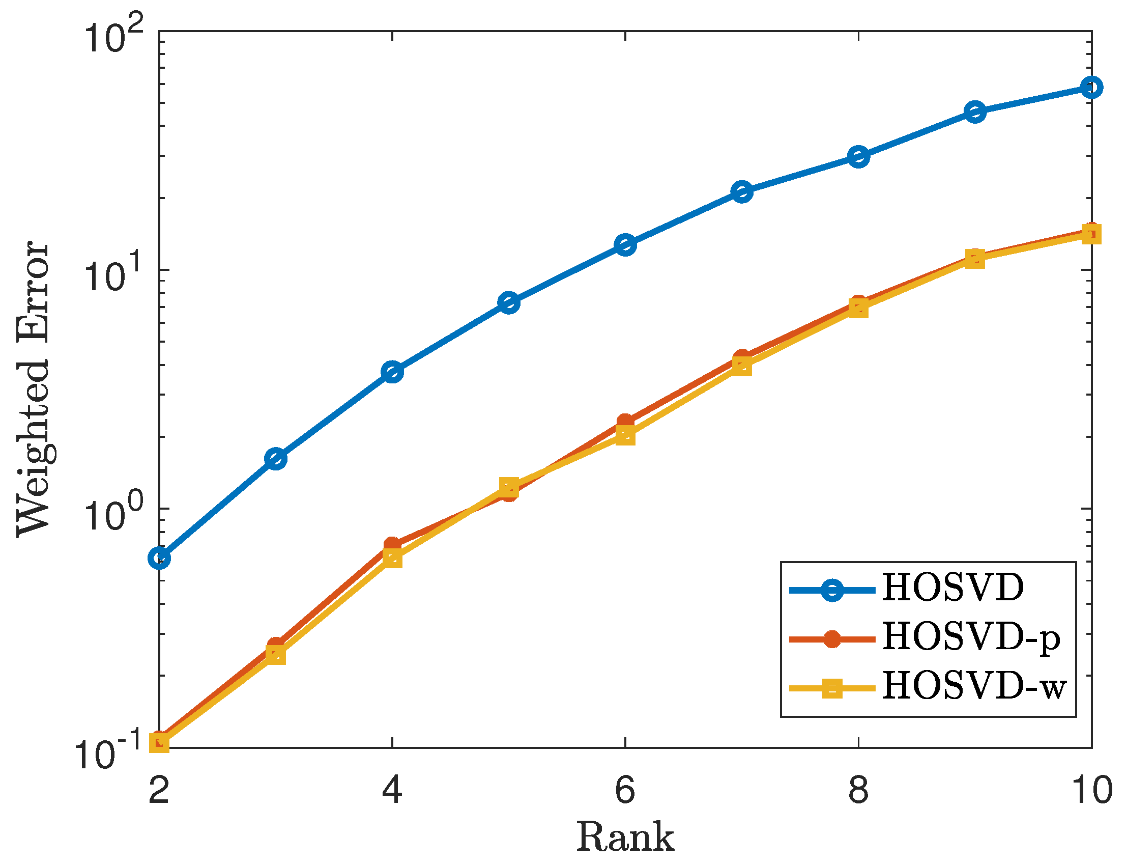
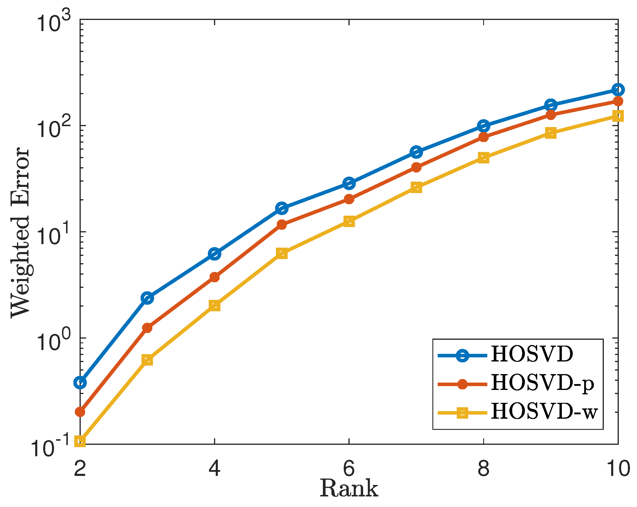
via the alternating least squares method for the non-negative CP decomposition. Next, we generate synthetic tensors $\mathcal{T}\in {\mathbb{R}}^{d_1\times \cdots \times d_n}$ of the form $\mathcal{C}{\times }_1{U}_1{\times }_2\cdots {\times }_n{U}_n$ with $n=3,4$ with $\mathrm{rank}\left({\mathcal{T}}_{\left(i\right)}\right)=r$, where $i=1,\cdots ,n$, and r varies from 2 to 10. Then we add mean zero Gaussion random noise $\mathcal{Z}$ with variance $\sigma ={10}^{-2}$ so that a new tensor is generated, which is denoted by $\mathcal{Y}=\mathcal{T}+\mathcal{Z}$. Then we solve the tensor completion problems (4), (5) and (6) by the HOSVD procedure. For each fixed low-rank tensor, we average over 20 tests. We measure error using the weighted Frobenius norm. The simulation results are reported in Figure 1 and Figure 2. Figure 1 shows the results for the tensor of size $100\times 100\times 100$ and Figure 2 shows the results for the tensor of size $50\times 50\times 30\times 30$, where the weighted error is of the form $\frac{\parallel {\mathcal{W}}^{(1/2)}⊡(\widehat{\mathcal{T}}-\mathcal{T}){\parallel }_F}{\parallel {\mathcal{W}}^{(1/2)}\parallel }$. These figures demonstrate that using our weighted samples performs more efficiently than using the original samples. For the uniform sampling case, the p weighted samples and $\mathcal{W}$ weighted samples exhibit similar performance.

4.2. Simulation for Non-Uniform Sampling Pattern

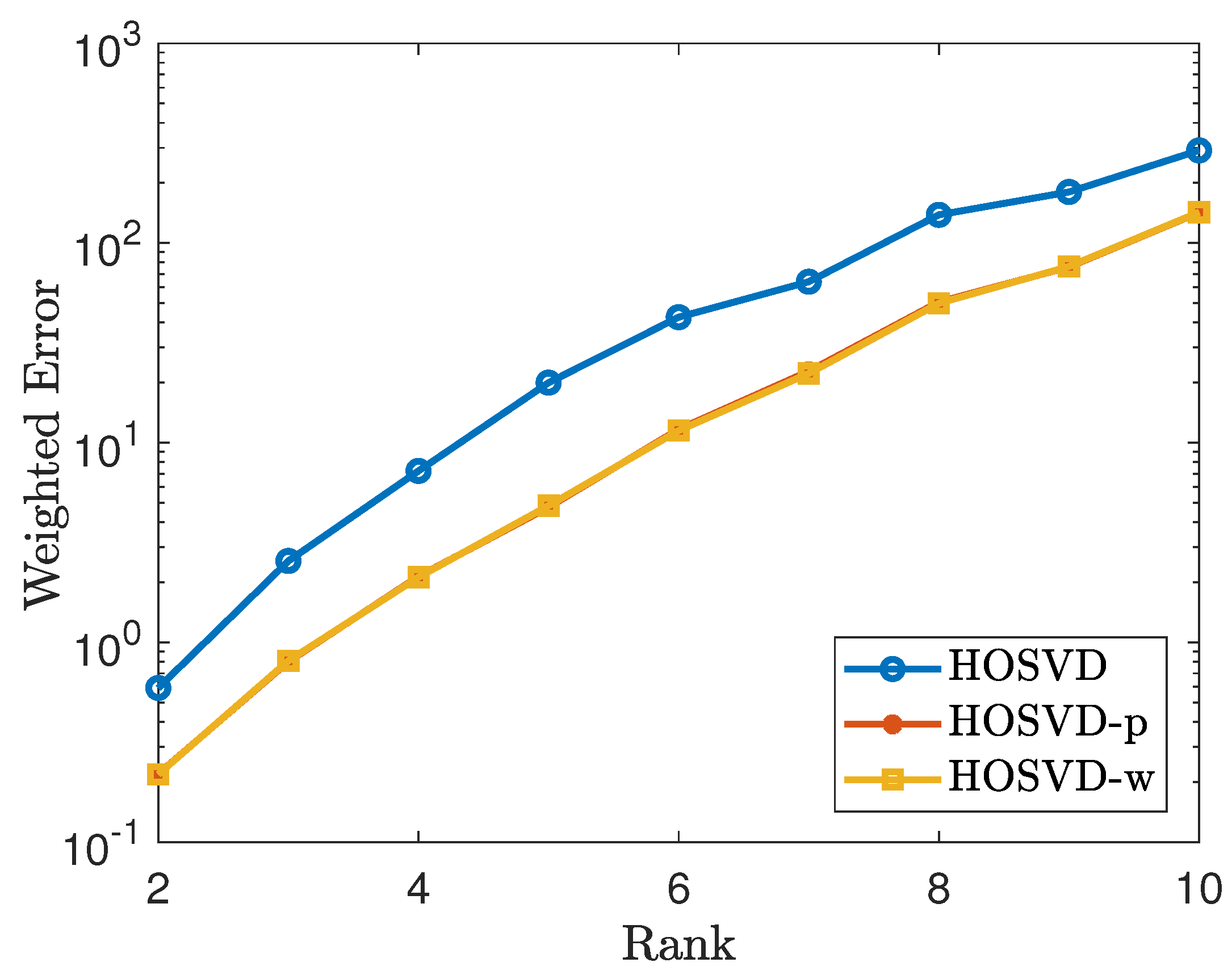
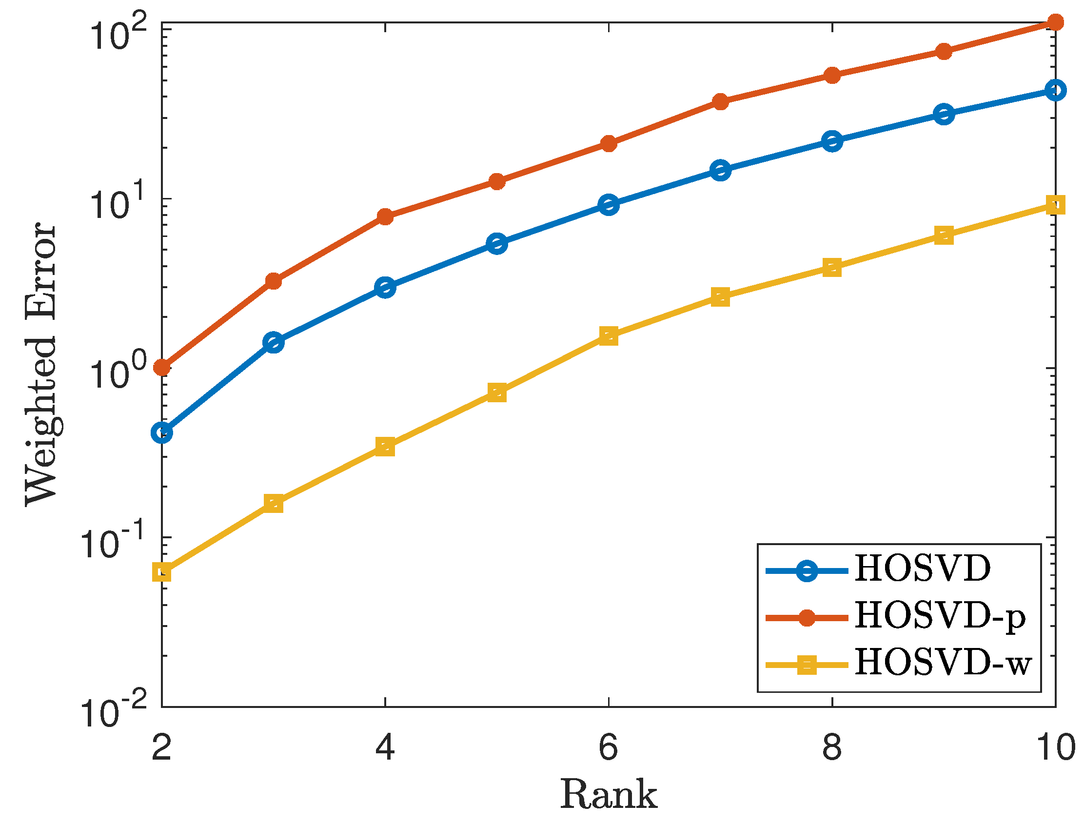
To generate a non-uniform sampling pattern with sampling rate $30\%$, we first generate a CP rank 1 tensor of the form $\mathcal{H}=〚\mathbf{1};{\mathit{h}}_{\mathbf{1}},\cdots ,{\mathit{h}}_{\mathit{n}}〛$, where ${\mathit{h}}_{\mathit{i}}=(u_i{\mathbf{1}}_{\lceil d_i/2\rceil },v_i{\mathbf{1}}_{\lfloor d_i/2\rfloor })$$0<u_i,v_i\le 1$. Let $\Omega \sim \mathcal{H}$. Then we repeat the process as in Section 4.1. The simulation results are shown in Figure 3 and Figure 4. As shown in figures, the results using our proposed weighted samples perform more efficiently than using the p weighted samples.

Remark 4.

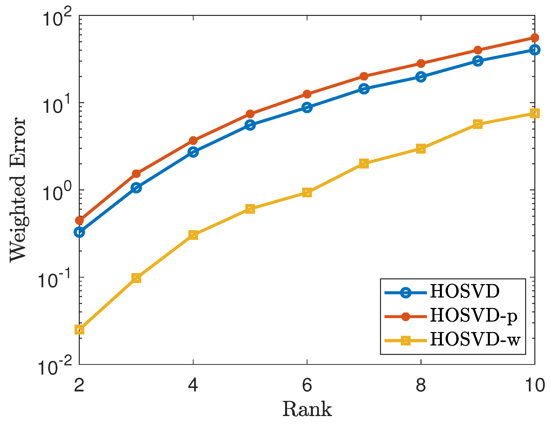
When we use the HOSVD procedure to solve (4), (5), and (6), we need (an estimate of) the Tucker rank as input. Instead of inputting the real rank of the true tensor, we could also use the rank that is estimated by considering the decay of the singular values for the unfolded matrices of the sampled tensor ${\mathcal{Y}}_{\Omega }$ as the input rank, which we call SV-rank. The simulation results for the non-uniform sampling pattern with SV-rank as input are reported in Figure 5. The simulation shows that the weighted HOSVD algorithm performs more efficiently than using the p weighted samples or the original samples. Comparing Figure 5 with Figure 3, we could observe that using the estimated rank as input for HOSVD procedure performs even better than using the real rank as input. This observation motivates a way to find a “good" rank as input for HOSVD procedure.

Remark 5.

We only provide guarantees on the performance in the weighted Frobenius norm, (as we report the weighted error $\frac{\parallel {\mathcal{W}}^{(1/2)}⊡(\widehat{\mathcal{T}}-\mathcal{T}){\parallel }_F}{\parallel {\mathcal{W}}^{(1/2)}{\parallel }_F}$), our procedures exhibit good empirical performance even in the usual relative error $\frac{\parallel \widehat{\mathcal{T}}{-\mathcal{T}\parallel }_F}{{\parallel \mathcal{T}\parallel }_F}$ when the Tucker rank of the tensor is relatively low. However, we observe that the advantages of weighted HOSVD scheme tend to be diminished in terms of relative error when the Tucker rank increases. This result is not surprising since the entries are treated unequally in scheme (6). Therefore we leave the investigation on relative error and the tensor rank for future work.

4.3. Test for Real Data

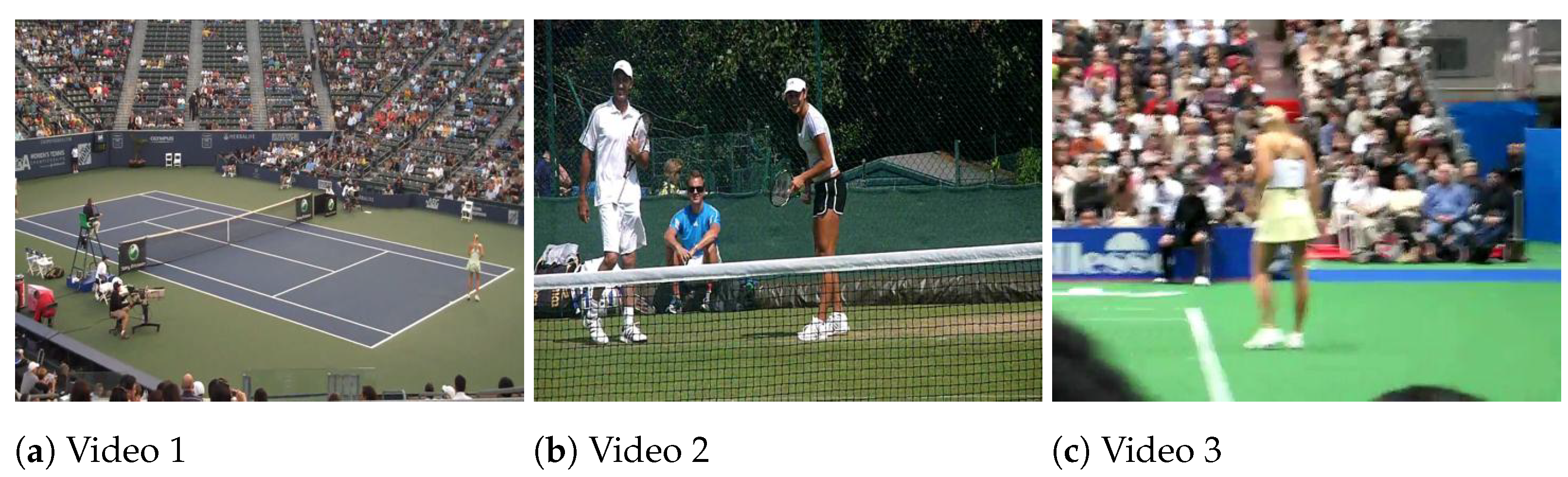
In this section, we test our weighted HOSVD algorithm for tensor completion on three videos, see [50]. The dataset is the tennis-serve data from an Olympic Sports Dataset [51]. One can download the dataset from http://vision.stanford.edu/Datasets (accessed date 10 May 2021). There are a lot of videos in the zip file and we only choose three of them: “d2P_zx_JeoQ_00120_00515.seq” (video 1), “gs3sPDfbeg4_00082_00229.seq”(video 2), and “VADoc-AsyXk_00061_ 0019.seq” (video 3). The three videos are color video. In our simulation, we use the same setup as the one in [50], and choose 30 frames evenly from each video. For each frame, the size is scaled to $360\times 480\times 3$, so each video is transformed into a 4-D tensor data of size $360\times 480\times 3\times 30$. The first frame of each video after preprocessing is illustrated in Figure 6.

We implement the experiments for different sampling rates of $10\%$, $30\%$, $50\%$, and $80\%$ to generate uniform and non-uniform sampling patterns $\Omega$. In our implementation, we use the SV-rank of ${\mathcal{T}}_{\Omega }$ as the input rank. According to the generated sampling pattern, we find a weight tensor $\mathcal{W}$ and find estimates ${\widehat{\mathcal{T}}}_1$ and ${\widehat{\mathcal{T}}}_2$ by considering (4) and (6) respectively, using the input Tucker rank $\mathit{r}$. The entries on ${\mathcal{T}}_1$ and ${\mathcal{T}}_2$ are forced to be the observed data. The Signal to Noise Ratio (SNR)

$$SNR\left(\widehat{\mathcal{T}}\right)=-20{log}_{10}\left(\frac{\parallel \widehat{\mathcal{T}}{-\mathcal{T}\parallel }_F}{{\parallel \mathcal{T}\parallel }_F}\right)$$

are computed and the simulation results are reported in

Table 1. Signal to noise ratio (SNR) and elapsed time (in second) for Higher Order Singular Value Decomposition (HOSVD) and HOSVD-w on video data with uniform sampling pattern. The HOSVD-w and HOSVD-p behave very similar for uniform sampling hence we integrate the results into one column.

Video	SR	Input Rank	HOSVD-w+TV	HOSVD	HOSVD-w/HOSVD-p	TVM
	10%	$\left[71735\right]$	13.29 (16.3 s)	1.27 (3.74 s)	10.15 (11.4 s)	13.04 (41.3 s)
	30%	$\left[181036\right]$	16.96 (14.0 s)	4.26 (4.01 s)	12.05 (7.23 s)	17.05 (29.7 s)
	50%	$\left[264311\right]$	19.60 (12.2 s)	8.21 (2.99 s)	14.59 (7.03 s)	19.68 (23.8 s)
	80%	$\left[4747322\right]$	24.90 (11.5 s)	17.29 (6.55 s)	19.75 (8.08 s)	25.01 (18.1 s)
	10%	$\left[28637\right]$	10.98 (13.1 s)	1.19 (4.20 s)	7.88 (8.76 s)	10.89 (42.2 s)
	30%	$\left[3418315\right]$	14.44 (16.1 s)	4.11 (3.80 s)	10.40 (7.51 s)	14.50 (31.4 s)
	50%	$\left[353339\right]$	16.95 (15.3 s)	7.85 (5.86 s)	12.84 (7.64 s)	16.96 (26.6 s)
	80%	$\left[5650321\right]$	22.21 (15.1 s)	16.51 (7.24 s)	18.64 (8.45 s)	22.19 (18.4 s)
	10%	$\left[129310\right]$	12.34 (16.1 s)	1.22 (2.73 s)	8.46 (9.88 s)	12.23 (45.7 s)
	30%	$\left[2024311\right]$	17.10 (15.3 s)	4.24 (3.17 s)	11.62 (7.62 s)	17.19 (35.3 s)
	50%	$\left[2532314\right]$	20.44 (12.3 s)	8.20 (3.92 s)	14.54 (5.85 s)	20.49 (28.9 s)
	80%	$\left[5072330\right]$	26.80 (12.4 s)	18.03 (8.40 s)	21.38 (8.93s)	26.71 (20.9 s)

and

Table 2. Signal to noise ratio (SNR) for HOSVD and HOSVD-w on video data with non-uniform sampling pattern.

Video	SR	Input Rank	HOSVD	HOSVD-w	HOSVD-p
	10%	$\left[61333\right]$	1.09	10.07	5.56
	30%	$\left[1028316\right]$	3.74	11.81	7.53
	50%	$\left[2141314\right]$	7.05	13.22	10.73
	80%	$\left[4457326\right]$	15.76	19.60	17.39
	10%	$\left[381132\right]$	1.13	8.04	4.33
	30%	$\left[2619316\right]$	3.79	10.13	6.80
	50%	$\left[3027310\right]$	7.15	12.57	10.14
	80%	$\left[5350323\right]$	14.81	18.55	16.31
	10%	$\left[161132\right]$	1.09	8.31	4.73
	30%	$\left[1723317\right]$	3.76	11.05	6.87
	50%	$\left[2438314\right]$	7.18	13.78	9.99
	80%	$\left[4769322\right]$	15.88	20.82	16.02

. As shown in the tables, applying HOSVD process to (6) can give a better result than applying HOSVD process to (4) directly regardless of the uniformity of the sampling pattern.

Finally, we test the proposed weighted HOSVD algorithm on real candle video data named “candle_4_A” [52] (The dataset can be downloaded from the Dynamic Texture Toolbox in http://0-www-vision-jhu-edu.brum.beds.ac.uk/code/ (accessed date 10 May 2021). We have tested the relation between the relative errors and the sampling rates using $\mathit{r}=(5,5,5)$ as the input rank for HOSVD algorithm. The relative errors are presented in Figure 7. The simulation results also show that the proposed weighted HOSVD algorithm can implement tensor completion efficiently.

4.4. The Application of Weighted HOSVD on Total Variation Minimization

As shown in the previous simulations, the weighted HOSVD decomposition can provide better results for tensor completion by comparing with HOSVD. There are a bunch of algorithms that are Sensitive to initialization. Additionally, real applications may have higher requirements for accuracy. Therefore, it is meaningful to combine our weighted HOSVD with other algorithms in order to further improve the performance. In this section, we would consider the application of weighted HOSVD decomposition on the total variation minimization algorithm. As a traditional approach, the total variation minimization (TVM), is broadly applied in studies about image recovery and denoising. While the earliest research could trace back to 1992 [53]. The later studies combined TVM and other low rank approximation algorithms such as Nuclear Norm Minimization (see e.g., [54,55,56]) and HOSVD (e.g., [57,58,59]) in order to achieve better performance in image and video completion tasks.

Motivated by the matrix TV minimization, we proposed the tensor TV minimization which is summarized in Algorithm 1. In Algorithm 1, the Laplacian operator computes the divergence of all-dimension gradients for each entry of the tensor. The shrink operator simply moves the input towards 0 with distance $\lambda$, or formally defined as:

$$\mathrm{shrink}(x,\lambda )=\mathbf{sign}\left(x\right)·max\left(\right|x|-\lambda ,0)$$

For the initialization of ${\mathcal{X}}^0$ in Algorithm 1, we assign ${\mathcal{X}}^0$ to be the output of the result from HOSVD-w.

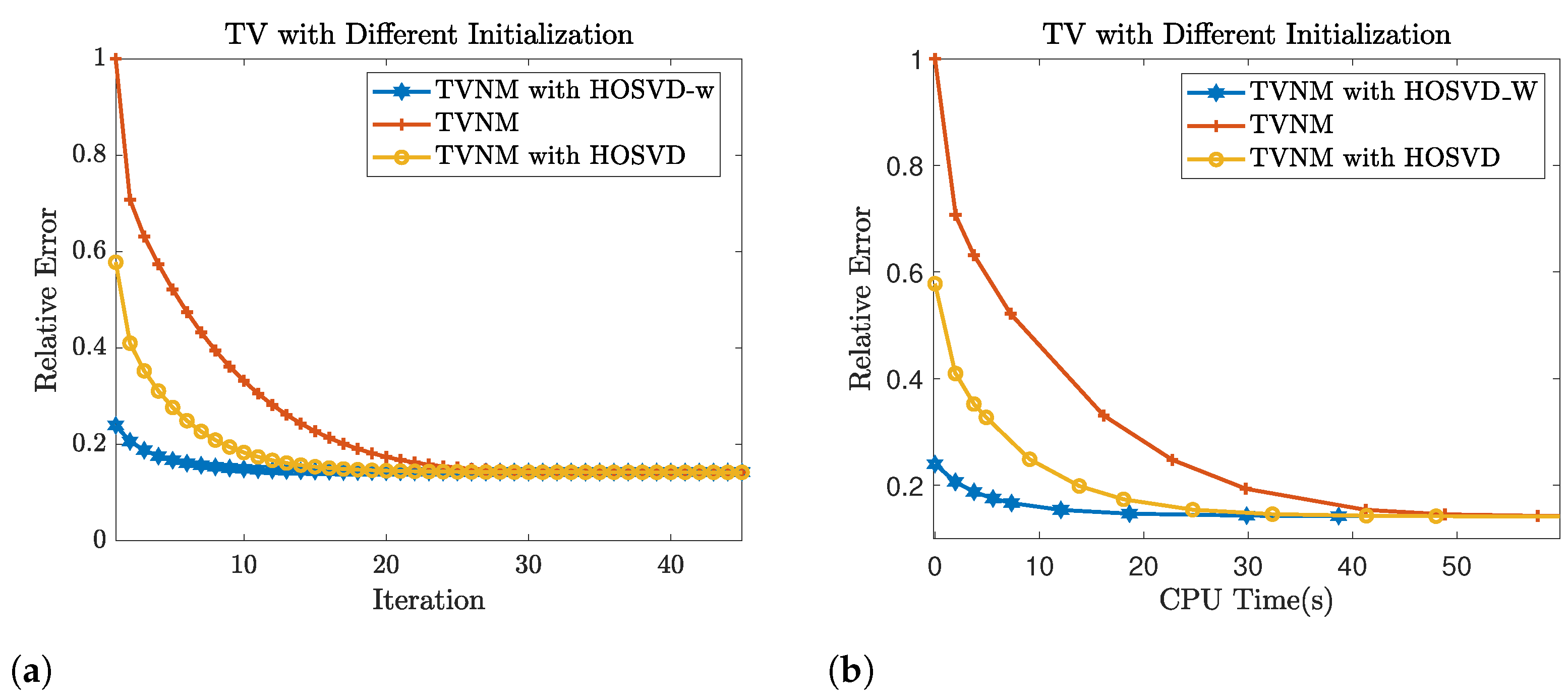
Applying the same experiment setting as in Section 4.3, we evaluate the performance of the cocktail approach as well as the regular HOSVD approach. We report the simulation results in Table 1 and we measure the performances by considering the signal to noise ratio(SNR). As shown in Table 1, the total variation minimization could be applied to further improve the result of (6). Specifically, the TVM with $\mathbf{0}$ as initialization performs similar to TVM with HOSVD-w as initialization when the observed rate is high, but the HOSVD-w initialization could improve the performance of TVM when the observed rate is very low (e.g., 10%). Additionally, we compared the decay of relative error for using the weighted HOSVD output as initialization and the default initialization (${\mathcal{X}}^0=\mathbf{0}$). The iterative results are shown in Figure 8, and it shows that using the result from weighted HOSVD as an initialization could notably reduce the iterations of TV-minimization for achieving the convergence threshold ($\parallel {\mathcal{X}}^k-{\mathcal{X}}^{k-1}{\parallel }_F<{10}^{-4}$).

Algorithm 1: TV Minimization for Tensor.

5. Conclusions

In this paper, we propose a simple but efficient algorithm named the weighted HOSVD algorithm for recovering an underlying low-rank tensor from noisy observations. For this algorithm, we provide upper and lower error bounds that measure the difference between the estimates and the true underlying low-rank tensor. The efficiency of our proposed weighted HOSVD algorithm is also shown by numerical simulations. Additionally, the result of our weighted HOSVD algorithm can be used as an initialization for the total variation minimization algorithm, which shows that using our method as an initialization for the total variation minimization algorithm can increasingly reduce the iterative steps leading to improved overall performance in reconstruction (see our conference paper [60]). It would be interesting for future work to combine the weighted HOSVD algorithm with other algorithms to achieve more accurate results for tensor completion in many settings.

References

- Hitchcock, F.L. The expression of a tensor or a polyadic as a sum of products. J. Math. Phys. 1927, 6, 164–189. [Google Scholar] [CrossRef]
- Kolda, T.G.; Bader, B.W. Tensor decompositions and applications. SIAM Rev. 2009, 51, 455–500. [Google Scholar] [CrossRef]
- Zare, A.; Ozdemir, A.; Iwen, M.A.; Aviyente, S. Extension of PCA to higher order data structures: An introduction to tensors, tensor decompositions, and tensor PCA. Proc. IEEE 2018, 106, 1341–1358. [Google Scholar] [CrossRef] [Green Version]
- Ge, H.; Caverlee, J.; Zhang, N.; Squicciarini, A. Uncovering the spatio-temporal dynamics of memes in the presence of incomplete information. In Proceedings of the 25th ACM International on Conference on Information and Knowledge Management, Indianapolis, IN, USA, 24–28 October 2016; pp. 1493–1502. [Google Scholar]
- Liu, J.; Musialski, P.; Wonka, P.; Ye, J. Tensor completion for estimating missing values in visual data. IEEE Trans. Pattern Anal. Mach. Intell. 2012, 35, 208–220. [Google Scholar] [CrossRef] [PubMed]
- Liu, Y.; Shang, F.; Cheng, H.; Cheng, J.; Tong, H. Factor matrix trace norm minimization for low-rank tensor completion. In Proceedings of the 2014 SIAM International Conference on Data Mining, Philadelphia, PA, USA, 24–26 April 2014; pp. 866–874. [Google Scholar]
- Song, Q.; Ge, H.; Caverlee, J.; Hu, X. Tensor Completion Algorithms in Big Data Analytics. ACM Trans. Knowl. Discov. Data 2019, 13, 1–48. [Google Scholar] [CrossRef]
- Kressner, D.; Steinlechner, M.; Vandereycken, B. Low-rank tensor completion by Riemannian optimization. BIT Numer. Math. 2014, 54, 447–468. [Google Scholar] [CrossRef] [Green Version]
- Ermiş, B.; Acar, E.; Cemgil, A.T. Link prediction in heterogeneous data via generalized coupled tensor factorization. Data Min. Knowl. Discov. 2015, 29, 203–236. [Google Scholar] [CrossRef]
- Symeonidis, P.; Nanopoulos, A.; Manolopoulos, Y. Tag recommendations based on tensor dimensionality reduction. In Proceedings of the 2008 ACM Conference on Recommender Systems, Lausanne, Switzerland, 23–25 October 2008; pp. 43–50. [Google Scholar]
- Cai, J.F.; Candès, E.J.; Shen, Z. A singular value thresholding algorithm for matrix completion. SIAM J. Optim 2010, 20, 1956–1982. [Google Scholar] [CrossRef]
- Cai, T.T.; Zhou, W.X. Matrix completion via max-norm constrained optimization. Electron. J. Stat. 2016, 10, 1493–1525. [Google Scholar] [CrossRef]
- Candes, E.J.; Plan, Y. Matrix completion with noise. Proc. IEEE 2010, 98, 925–936. [Google Scholar] [CrossRef] [Green Version]
- Candès, E.J.; Recht, B. Exact matrix completion via convex optimization. Found. Comput. Math. 2009, 9, 717. [Google Scholar] [CrossRef] [Green Version]
- Amit, Y.; Fink, M.; Srebro, N.; Ullman, S. Uncovering shared structures in multiclass classification. In Proceedings of the 24th International Conference on Machine Learning, Corvalis, OR, USA, 20–24 June 2007; pp. 17–24. [Google Scholar]
- Cai, H.; Cai, J.F.; Wang, T.; Yin, G. Accelerated Structured Alternating Projections for Robust Spectrally Sparse Signal Recovery. IEEE Trans. Signal Process. 2021, 69, 809–821. [Google Scholar] [CrossRef]
- Gleich, D.F.; Lim, L.H. Rank aggregation via nuclear norm minimization. In Proceedings of the 17th ACM SIGKDD International Conference on Knowledge Discovery and Data Mining, San Diego, CA, USA, 21–24 August 2011; pp. 60–68. [Google Scholar]
- Liu, Z.; Vandenberghe, L. Interior-point method for nuclear norm approximation with application to system identification. SIAM J. Matrix Anal. Appl. 2009, 31, 1235–1256. [Google Scholar] [CrossRef]
- Foucart, S.; Needell, D.; Pathak, R.; Plan, Y.; Wootters, M. Weighted matrix completion from non-random, non-uniform sampling patterns. IEEE Trans. Inf. Theory 2020, 67, 1264–1290. [Google Scholar] [CrossRef]
- Bhojanapalli, S.; Jain, P. Universal matrix completion. arXiv 2014, arXiv:1402.2324. [Google Scholar]
- Heiman, E.; Schechtman, G.; Shraibman, A. Deterministic algorithms for matrix completion. Random Struct. Algorithms 2014, 45, 306–317. [Google Scholar] [CrossRef]
- Li, Y.; Liang, Y.; Risteski, A. Recovery guarantee of weighted low-rank approximation via alternating minimization. In Proceedings of the International Conference on Machine Learning, New York, NY, USA, 19–24 June 2016; pp. 2358–2367. [Google Scholar]
- Pimentel-Alarcón, D.L.; Boston, N.; Nowak, R.D. A characterization of deterministic sampling patterns for low-rank matrix completion. IEEE J. Sel. Top. Signal Process. 2016, 10, 623–636. [Google Scholar] [CrossRef] [Green Version]
- Shapiro, A.; Xie, Y.; Zhang, R. Matrix completion with deterministic pattern: A geometric perspective. IEEE Trans. Signal Process. 2018, 67, 1088–1103. [Google Scholar] [CrossRef] [Green Version]
- Ashraphijuo, M.; Aggarwal, V.; Wang, X. On deterministic sampling patterns for robust low-rank matrix completion. IEEE Signal Process. Lett. 2017, 25, 343–347. [Google Scholar] [CrossRef] [Green Version]
- Ashraphijuo, M.; Wang, X.; Aggarwal, V. Rank determination for low-rank data completion. J. Mach. Learn. Res. 2017, 18, 3422–3450. [Google Scholar]
- Pimentel-Alarcón, D.L.; Nowak, R.D. A converse to low-rank matrix completion. In Proceedings of the 2016 IEEE International Symposium on Information Theory (ISIT), Barcelona, Spain, 10–15 July 2016; pp. 96–100. [Google Scholar]
- Chatterjee, S. A deterministic theory of low rank matrix completion. arXiv 2019, arXiv:1910.01079. [Google Scholar]
- Király, F.J.; Theran, L.; Tomioka, R. The algebraic combinatorial approach for low-rank matrix completion. arXiv 2012, arXiv:1211.4116. [Google Scholar]
- Eftekhari, A.; Yang, D.; Wakin, M.B. Weighted matrix completion and recovery with prior subspace information. IEEE Trans. Inf. Theory 2018, 64, 4044–4071. [Google Scholar] [CrossRef] [Green Version]
- Negahban, S.; Wainwright, M.J. Restricted strong convexity and weighted matrix completion: Optimal bounds with noise. J. Mach. Learn. Res. 2012, 13, 1665–1697. [Google Scholar]
- Lee, T.; Shraibman, A. Matrix completion from any given set of observations. In Proceedings of the Advances in Neural Information Processing Systems, Red Hook, NY, USA, 5–10 December 2013; pp. 1781–1787. [Google Scholar]
- Gandy, S.; Recht, B.; Yamada, I. Tensor completion and low-n-rank tensor recovery via convex optimization. Inverse Probl. 2011, 27, 025010. [Google Scholar] [CrossRef] [Green Version]
- Ashraphijuo, M.; Wang, X. Fundamental conditions for low-CP-rank tensor completion. J. Mach. Learn. Res. 2017, 18, 2116–2145. [Google Scholar]
- Barak, B.; Moitra, A. Noisy tensor completion via the sum-of-squares hierarchy. In Proceedings of the Conference on Learning Theory, New York, NY, USA, 23–26 June 2016; pp. 417–445. [Google Scholar]
- Jain, P.; Oh, S. Provable tensor factorization with missing data. In Proceedings of the Advances in Neural Information Processing Systems, Montreal, QC, Canada, 8–13 December 2014; pp. 1431–1439. [Google Scholar]
- Goldfarb, D.; Qin, Z. Robust low-rank tensor recovery: Models and algorithms. SIAM J. Matrix Anal. Appl. 2014, 35, 225–253. [Google Scholar] [CrossRef] [Green Version]
- Mu, C.; Huang, B.; Wright, J.; Goldfarb, D. Square deal: Lower bounds and improved relaxations for tensor recovery. In Proceedings of the International Conference on Machine Learning, Beijing, China, 21–26 June 2014; pp. 73–81. [Google Scholar]
- Hitchcock, F.L. Multiple invariants and generalized rank of a p-way matrix or tensor. J. Math. Phys. 1928, 7, 39–79. [Google Scholar] [CrossRef]
- Kruskal, J.B. Rank, decomposition, and uniqueness for 3-way and N-way arrays. In Multiway Data Analysis; North-Holland Publishing Co.: Amsterdam, The Netherlands, 1989; pp. 7–18. [Google Scholar]
- Acar, E.; Yener, B. Unsupervised multiway data analysis: A literature survey. IEEE Trans. Knowl. Data Eng. 2008, 21, 6–20. [Google Scholar] [CrossRef]
- Sidiropoulos, N.D.; De Lathauwer, L.; Fu, X.; Huang, K.; Papalexakis, E.E.; Faloutsos, C. Tensor decomposition for signal processing and machine learning. IEEE Trans. Signal Process. 2017, 65, 3551–3582. [Google Scholar] [CrossRef]
- Carroll, J.D.; Chang, J.J. Analysis of individual differences in multidimensional scaling via an N-way generalization of “Eckart-Young” decomposition. Psychometrika 1970, 35, 283–319. [Google Scholar] [CrossRef]
- Bro, R. PARAFAC. Tutorial and applications. Chemom. Intell. Lab. Syst. 1997, 38, 149–172. [Google Scholar] [CrossRef]
- Kiers, H.A.; Ten Berge, J.M.; Bro, R. PARAFAC2—Part I. A direct fitting algorithm for the PARAFAC2 model. J. Chemometr. 1999, 13, 275–294. [Google Scholar] [CrossRef]
- Tomasi, G.; Bro, R. PARAFAC and missing values. Chemom. Intell. Lab. Syst. 2005, 75, 163–180. [Google Scholar] [CrossRef]
- Tucker, L.R. Some mathematical notes on three-mode factor analysis. Psychometrika 1966, 31, 279–311. [Google Scholar] [CrossRef] [PubMed]
- De Lathauwer, L.; De Moor, B.; Vandewalle, J. A multilinear singular value decomposition. SIAM J. Matrix Anal. Appl. 2000, 21, 1253–1278. [Google Scholar] [CrossRef] [Green Version]
- Kroonenberg, P.M.; De Leeuw, J. Principal component analysis of three-mode data by means of alternating least squares algorithms. Psychometrika 1980, 45, 69–97. [Google Scholar] [CrossRef]
- Fang, Z.; Yang, X.; Han, L.; Liu, X. A sequentially truncated higher order singular value decomposition-based algorithm for tensor completion. IEEE Trans. Cybern. 2018, 49, 1956–1967. [Google Scholar] [CrossRef] [PubMed]
- Niebles, J.C.; Chen, C.W.; Li, F.F. Modeling temporal structure of decomposable motion segments for activity classification. In European Conference on Computer Vision; Springer: Berlin/Heidelberg, Germany, 2010; pp. 392–405. [Google Scholar]
- Ravichandran, A.; Chaudhry, R.; Vidal, R. Dynamic Texture Toolbox. 2011. Available online: http://www.vision.jhu.edu (accessed on 10 May 2021).
- Rudin, L.I.; Osher, S.; Fatemi, E. Nonlinear total variation based noise removal algorithms. Phys. D Nonlinear Phenom. 1992, 60, 259–268. [Google Scholar] [CrossRef]
- Wu, Z.; Wang, Q.; Jin, J.; Shen, Y. Structure tensor total variation-regularized weighted nuclear norm minimization for hyperspectral image mixed denoising. Signal Process. 2017, 131, 202–219. [Google Scholar] [CrossRef]
- Madathil, B.; George, S.N. Twist tensor total variation regularized-reweighted nuclear norm based tensor completion for video missing area recovery. Inf. Sci. 2018, 423, 376–397. [Google Scholar] [CrossRef]
- Yao, J.; Xu, Z.; Huang, X.; Huang, J. Accelerated dynamic MRI reconstruction with total variation and nuclear norm regularization. In International Conference on Medical Image Computing and Computer-Assisted Intervention; Springer: Berlin/Heidelberg, Germany, 2015; pp. 635–642. [Google Scholar]
- Wang, Y.; Peng, J.; Zhao, Q.; Leung, Y.; Zhao, X.L.; Meng, D. Hyperspectral image restoration via total variation regularized low-rank tensor decomposition. IEEE J. Sel. Top. Appl. Earth Obs. Remote Sens. 2017, 11, 1227–1243. [Google Scholar] [CrossRef] [Green Version]
- Ji, T.Y.; Huang, T.Z.; Zhao, X.L.; Ma, T.H.; Liu, G. Tensor completion using total variation and low-rank matrix factorization. Inf. Sci. 2016, 326, 243–257. [Google Scholar] [CrossRef]
- Li, X.; Ye, Y.; Xu, X. Low-rank tensor completion with total variation for visual data inpainting. In Proceedings of the AAAI Conference on Artificial Intelligence, San Francisco, CA, USA, 4–9 February 2017; Volume 31. [Google Scholar]
- Chao, Z.; Huang, L.; Needell, D. Tensor Completion through Total Variation with Initialization from Weighted HOSVD. In Proceedings of the Information Theory and Applications, San Diego, CA, USA, 2–7 February 2020. [Google Scholar]
- Tropp, J.A. User-friendly tail bounds for sums of random matrices. Found. Comput. Math. 2012, 12, 389–434. [Google Scholar] [CrossRef] [Green Version]
- Lancaster, P.; Farahat, H. Norms on direct sums and tensor products. Math. Comp. 1972, 26, 401–414. [Google Scholar] [CrossRef]
Figure 1.
Tensor of size using the uniform sampling pattern: plots the errors of the form . The lines labeled as HOSVD, HOSVD-p and HOSVD-w represent the results for solving (4), (5) and (6), respectively.
Figure 2.
Figure 3.
Tensor of size using the non-uniform sampling pattern: plots the errors of the form . The lines labeled as HOSVD, HOSVD-p and HOSVD-w represent the results for solving (4), (5) and (6), respectively.
Figure 4.
Figure 5.
Tensor of size using the non-uniform sampling pattern and with the SV-rank as the input rank: plots the errors of the form .
Figure 6.
The first frame of videos [50].
Figure 7.
Relation between relative error and sampling rate for the dataset “candle_4_A” using as the input rank for HOSVD process. The left figure records the relative error for the uniform sampling pattern and the right figure for the non-uniform sampling pattern. The sampling error stands for the relative error between the original video and the video with masked entries estimated to be zeros, hence should approximately equal to , where SR is the sampling rate.
Figure 8.
Convergence comparison between total variation minimization (TVM) with HOSVD-w, , and HOSVD as initialization on video 1 with SR = 50%: (a) the relative error vs. number of iterations. (b) the relative error v.s. total computational CPU time(initialization + completion).