Predicting Traffic and Risk Exposure in the Maritime Industry

1
School of Population and Global Health, University of Western Australia, Perth 6009, Australia
2
Econometric Institute, Erasmus School of Economics, Erasmus University Rotterdam, 3062 Rotterdam, The Netherlands
*
Author to whom correspondence should be addressed.
Safety 2019, 5(3), 42; https://0-doi-org.brum.beds.ac.uk/10.3390/safety5030042
Submission received: 26 March 2019
/
Revised: 29 May 2019
/
Accepted: 27 June 2019
/
Published: 1 July 2019
(This article belongs to the Special Issue Maritime Safety and Operations)
Abstract
:Maritime regulators, port authorities, and industry require the ability to predict risk exposure of shipping activities at a micro and macro level to optimize asset allocation and to mitigate and prevent incidents. This article introduces the concept of a strategic planning tool by making use of the multi-layered risk estimation framework (MLREF), which accounts for ship specific risk, vessel traffic densities, and meets ocean conditions at the macro level. This article’s main contribution is to provide a traffic and risk exposure prediction routine that allows the traffic forecast to be distributed across the shipping route network to allow for predicting scenarios at the macro level (e.g., covering larger geographic areas) and micro level (e.g., passage way, particular route of interest). In addition, the micro level is introduced by providing a theoretical idea to integrate location specific spatial rate ratios along with the effect of the risk control option to perform sensitivity analysis of risk exposure prediction scenarios. Aspects of the risk exposure estimation routine were tested via a pilot study for the Australian region using a comprehensive and unique combination of datasets. Sources of uncertainties for risk assessments are described in general and discussed along with the potential for future developments and improvements.
1. Introduction
Incidents in shipping can lead to high costs and pollution damage to society. These costs vary substantially as demonstrated by several selected examples of oil spills including the Exxon Valdez (1989) with $USD 95B, the Sea Empress (1996) with £62M, and the Prestige (2002) with €778M. [1] The overall goal of any regulatory authority such as maritime administration or port authority is to assess and predict risk exposure in order to enhance the selection and deployment of risk control options (RCO’s) such as vessel traffic management, improved surveillance, aids to navigation, pilotage, inspections and surveys, and emergency responses. This allows improved asset allocation at the strategic level but also enhances surveillance to prevent incidents from happening at the operational level. Risk exposure can be expressed using different metrics such as expected numbers of incidents leading to a very serious and serious accident. This can also be converted into a monetary value at risk (MVR). MVR is best understood as a monetary value that can be used as proxy for incident consequences that are difficult to quantify. Wood [2] identifies four components to the costs of marine incidents, such as lost assets, loss of cargo, lost lives, and pollution. It is very complex to estimate some of these components since one cannot put a monetary value to the loss or damage to marine ecology (Goulielmos and Giziakis [3], Grigalunas et al. [4], and Grey [5]). The Formal Safety Assessment Guidelines provide an overall framework to address the various risks and consequences but does not provide any details to deal with damages to the marine ecology that cannot be quantified in monetary terms. Cost benefit analysis and the evaluation of risk control options are primarily based on costs to human lives and property IMO [6], which is understandable given that the main scope of Formal Safety Assessment (FSA) studies is to provide evidence when big revisions to the legislative framework are proposed at the international level, which is always a compromise. At the individual country level, however, a maritime administration might choose to be stricter and perform strategic planning that will allow a more refined allocation of its assets to avert incidents from happening in the first place. The main emphasis is not directly related to consequences but rather incident prevention that can lead to potential high consequences such as collisions and groundings where the associated damage types are mentioned by Wood [2]. The layers presented, in this case, as part of the strategic planning tool, cover the various components mentioned in the FSA methodology of the IMO but provide a more refined approach for coastal states for medium to long term strategic planning aspects and incident prevention.
This approach builds on the initial work of Vander Hoorn and Knapp [7] who introduce the multi-layered risk estimation framework (MLREF) to estimate risk exposure and provide a framework to expand on the various shortcomings of current risk assessments. While Vander Hoorn and Knapp [7] demonstrate the potential use of the framework as part of a strategic planning tool (SPT), components were still missing at the time, such as a method to predict risk exposure given changes in underlying traffic or the integration of location specific correction factors for collisions, powered groundings, or drift groundings that allow the application of MLREF at a more local level. The ability to allow for different metrics to measure risk exposure that indirectly accounts for potential incident damage type consequences also needs further refinement.
The contribution of this article is to introduce a method to predict traffic densities and subsequently risk exposure and to discuss the integration of a spatial correction factor as well as further discuss other extensions to account for consequences in a more refined way. The results of a pilot project with the Australian Maritime Safety Authority (AMSA) demonstrates the practical application of the traffic density and risk exposure prediction routine for regions of interest: the Great Barrier Reef (GBR), the North West (NW), and the South West (SW) regions of Australia.
Current approaches for risk assessment in shipping show serious limitations. Application areas are either geared toward semi real-time operational aspects (Hueffmeier et al. [8], and Eide et al. [9]) or small areas using a micro-level approach or medium to long term strategic planning aspects with limited prediction ability (DNV [10], BRISK [11], and Hansen et al. [12]). In addition, changes in location and magnitude of risk given future traffic scenarios are not quantified since the emphasis is primarily on real-time or near-real time applications (Montewka et al. [13]). Neither line of approach allows the integration of fully automated routines in order to quantify risk exposure. More importantly, risk is primarily estimated by modelling the geometry of the traffic and ignores the individual safety qualities of vessels. As such, vessels are treated equally, which is unrealistic given that safety qualities of vessels can vary considerably (Heij and Knapp [14], Heij et al. [15], and Knapp [16]) and are the reason why port state control inspections or industry vetting inspections exist. If incident data are used in the current approaches, it is not combined from various sources and biases and can, therefore, influence the validity of results.
Another shortcoming of current methods used in the industry is that the underlying location-specific environmental criteria such as the effect of wind, wave, and currents are omitted due to the complexities involved in quantifying their effect on risk exposure. Furthermore, uncertainties in the estimates are not identified nor quantified (Merrick and van Dorp [17]). Previous approaches to model location-specific probabilities of oil spills provide very different results (Goerlandt and Stahlberg [18]) and demonstrate the difficulty in providing reliable answers. The lack of understanding of the sources and magnitude of uncertainties makes it difficult for regulators to make policy decisions in order to reduce risk to an acceptable level.
2. Materials and Methods
2.1. High Level Description of the Components of the Strategic Planning Tool
Based on Vander Hoorn and Knapp [7], total risk exposure can be described as the combination of risk layers as follows: (1) ship specific risk as a proxy to safety quality, (2) vessel traffic densities, (3) location specific physical environmental parameters such as wind, wave, currents, and bathymetry, (4) other environmental factors such as sensitivities to pollution, and (5) intervention effects of risk control options (RCO), which can be deployed to mitigate risk such as e.g., pilotage, emergency towing tugs, VTS, SRS, navigational aids, and inspections. Total risk exposure is defined as the integration of these risk layers in order to assess and predict risk exposure for a given area of interest.
Figure 1 provides the components of MLREF (left hand side) as well as the visualization of a generic use case scenario of the proposed SPT. Risk exposure endpoints are collisions, which are powered and drift groundings leading to a very serious and serious incidents as well as candidates (irrespective of seriousness). Endpoints can be extended in future applications. In particular, the integration of estimating risk exposure in monetary terms to provide a proxy to consequences as demonstrated by Vander Hoorn and Knapp [7], which included oil pollution or ship emissions.
For strategic planning, the time frame is medium to long term, e.g., next five, 10, or 15 years. The end user can choose an area of interest, an economic or business scenario (e.g., business as usual, good economy, bad economy) and a time frame for future predictions. Other aspects such as change in traffic composition (e.g., size of vessels) can be chosen. Based on the user input parameters, the system calculates a baseline risk and future prediction scenarios where the magnitude and location of change of risk exposure is most relevant.
The end user can then perform sensitivity analysis given the effect and combination of control options (RCO) to find the best combination to mitigate risk, save money with improved asset allocation, or make policy decisions. Examples for asset allocations could be (1) verification of pollution response resources and arrangements, (2) verification of emergency towage asset location, (3) ship inspection resource allocation, and (4) placement or evaluation of navigational aids. Policy related topics could be to (1) assess/minimize emissions, (2) ad-hoc input into policy formulation in general, (3) introduction of new ship routing measures, and (4) visualizations such as change in traffic densities and/or risk exposure over time.
As mentioned earlier, the risk exposure endpoints at this stage are collisions, powered and drift groundings, and can be measures in various ways such as probabilities, expected numbers of incidents, and the monetary value at risk (MVR) as proxy to consequences (Knapp and Heij [14]). If incident costs are also considered as endpoints, then cost/benefit analysis can be performed. The developed routine should provide an estimate of the uncertainties when possible.
One major difference to other approaches is that, in combining the first two layers provided in Figure 1, the individual safety quality of a vessel is captured in addition to vessel traffic densities rather than estimating risk based on the geometry of vessel traffic. It is believed that 80% of all navigational incidents are somehow related to human error (Hansen [12]). Hence, the safety quality of a particular vessel is assumed to be more important in most incident cases.
The next section provides the theoretical framework for development of the risk prediction routine of the SPT and the integration of spatial correction factors so that the SPT can be used for macro and micro level applications. The routine was developed within a pilot project in conjunction with AMSA and relevant aspects are described and presented.
2.2. Theoretical Framework for Predictions at the Macro and Micro Level
The proposed method builds on the ideas presented by Vander Hoorn and Knapp [7] to combine ship-specific risk and vessel traffic densities based on nautical miles travelled, which works well at the macro level such as large geographic areas and where the micro level risk such as risk exposure at a specific route is not needed. The routine is extended by providing a risk prediction routine needed to run prediction scenarios for the SPT and by proposing an extension to integrate spatial correction factors so that the routine can also be used at the micro level. The aim is to evaluate current risk and to predict how the location and magnitude of risk exposure will change given an increase in future traffic, e.g., five, 10, or 15 years. Uncertainties are identified and discussed when possible.
Vander Hoorn and Knapp [7] aggregate individual ship-specific risk with total traffic densities measured as distance travelled to derive risk exposure at the grid level, which can then be aggregated across large areas. Comparisons of this macro style method have shown that this works well at predicting numbers of incidents across a large area such as Australia’s Exclusive Economic Zone (EEZ). Ship-specific risk as a proxy to safety quality is based on Knapp [16,19] using binary logistic regression. The statistical models are based on a unique combination of data sources (IMO, IHS Markit, LLIS, AMSA) of five years of data regarding ship particulars of the world fleet, their changes over time, global incident, and PSC inspections. Approximately 500 variables have been tested and separate models are estimated for each incident type and seriousness if possible. Incident seriousness is classified based on IMO definitions (IMO [20]). Please refer to Appendix A for a high-level summary of the logit models.
To provide traffic and risk prediction routines in order to estimate the magnitude and location of change in future risk exposure via prediction scenarios of the SPT. A risk prediction routine needs to be developed, which translates future vessel arrivals in port into risk exposure across areas.
Since risk exposure predictions are based on traffic projections, a traffic projection routine is proposed and tested in a pilot project setup as proof of concept. It consists of a ship tracks from automatic identification system (AIS) data, a route network (RouteNet), and a voyage database. Traffic data from AIS is matched against a route network, which provides the entry/exit points of the area of interest and accounts for all possible routes of the entry/exit points to major points capturing around 80% of total traffic. The purpose of establishing a voyage database is to facilitate generating a counterfactual traffic density based on an alternative scenario, e.g., traffic flow, pattern, and vessel composition in the future (e.g., 2020, 2025). The voyage database is then analyzed to study aggregate level spatial features of traffic, e.g., regional level patterns (aggregated over the year), and also enable spatial risk assessment.
Each ship track in the voyage database is classified according to its ship type and voyage description, i.e., origin and destination along with additional summary information such as distance travelled, days at sea, etc. At a very basic level, one could assume vessels follow routes as defined on the RouteNet. Implemented in this way, expected traffic volume and pattern under a counterfactual scenario can be extracted by simply applying the full set of port arrival forecasts to the RouteNet and proceeding with the risk assessment. Further details on the voyage database and RouteNet are provided in Appendix B.
Besides the traffic projections and, if the strategic planning tool is used at the micro level such as specific routes or smaller regions, then location specific parameters need to be accounted for. A spatial adjustment can also be considered if the data are available to reflect relative differences in risk between areas. More formally, this is implemented by first defining risk for an individual voyage as:
where:
- is the annual accident probability for vessel i (based on a vessel with ship particulars equal to that of vessel i),
- is the nautical miles travelled during voyage j of vessel i,
- is the expected total nautical miles travelled for vessel i (based on the expected nautical miles travelled for the vessels of this type).
Note that distance travelled is used, in this case, as a proxy for calculating risk exposure. In principle, there will be many metrics that can be considered in this step such as days at sea, frequency of collision candidates, etc. Defined in this way, the assumption is made that the effect of ship-specific risk factors for vessels observed in the study region is the same as the global ship-level risk but scaled (down), according to the fraction of traffic exposure. In other words, a baseline risk for a given level and type of traffic based on incident models estimated on global incident data is defined and applied at the individual voyage level. The baseline rate of accidents for ships of type k, and which enter location s, can be obtained using the equation below.
where:
- is the baseline probability for voyage j of ship i having an accident at location s. Spatial differences in risk between areas could be incorporated by:
- is an estimator for the spatial rate ratio at location s.
The spatial rate ratio can refine macro level results and provide an avenue to make predictions at a micro level. In other words, baseline risk exposure is adjusted based on geographic and location-specific conditions. At this stage, a spatial rate ratio for collisions and powered grounding still needs to be developed and a separate project is currently dealing with this aspect. Possible metrics could be developed using AIS data, geographic information systems (GIS) data, or drift simulations. For collisions, a metric that quantifies traffic complexity such as course orientations, crossing of vessels, or speed could be used. For powered groundings, speed, and distance to a hazard is more relevant. This could be accomplished via the creation of an available sea-room layer by combining bathymetry and extracts of electronic charts. This available sea-room layer could measure the distance to a hazard horizontally and vertically.
For drift grounding, location-specific conditions influence the probability of grounding given that the vessel is drifting due to the vessel’s exposure to the effect of wind, waves, and currents on the hull of a drifting vessel. A spatial rate ratio could be introduced via drift simulations and by adopting an approach suggested by Eide et al. [9] where the frequency of drift grounding is modelled to be the product of the frequency of ship drift candidates and the probability of grounding given that the ship is adrift. This is further influenced by the probability of self-repair, the time to shore probability distribution, and the tug response time as well as the possibility of anchoring. Preliminary tests were performed using three years of drift simulations, but results were not found to be suitable at this stage to be further processed since the test area was too small.
Traffic density under a counterfactual (future) scenario can be predicted as follows. Let Dkp(s) represent a baseline port level traffic density quantified as total nautical miles travelled (per 1000 vessels) at location s after aggregating across all j voyages of ship type k into/out of port p. Then we define:
where:
- represents the traffic density at location s under counterfactual scenario c for ship type k.
The double counting of vessels travelling between ports is avoided in this calculation, i.e., a vessel that travels from one port to another is not counted twice as both an arrival and a departure. The calculation involves the product sum across all ports of the port level density the number of voyages for ship type k [ to/from a port (in multiples of 1000), and the relative rate of change in numbers of voyages for ship type k between the baseline traffic density and the counterfactual scenario, which is estimated from the arrival forecast data.
In Equation (4), P + 1 represents the case whereby a vessel enters the area of interest but then bypasses all major ports defined on the route net. The traffic density for P + 1 represents a relatively small proportion of all voyages, but is needed here to capture total vessel activity.
The counterfactual traffic density is not calculated at the route level, i.e., it is based on scaling total traffic flows at the port level. In theory, it would be possible to extend the method described in this case so that any differences in relative changes at the route level can be reflected in the counterfactual density. However, this would only be necessary if general traffic patterns along major routes for a selected port/ship type pair were expected to change at different rates. Preliminary analyses of data provided via the pilot project did not reveal that to be the case for Australia. In the future, estimation of the baseline traffic density should be established with a larger baseline period such as three to five years instead of one year only, as used in the pilot study. This would also give a more accurate assessment of baseline risk.
Under the above approach, new routes could be added, and existing routes could be removed from evaluation of the counterfactual traffic density. The total density under the counterfactual scenario can then be derived by Equation (5) below.
Under a counterfactual traffic scenario (e.g., traffic in 2025), the rate of accidents for ship type (ST) equal k can be obtained by the equations below.
where:
- is an estimator of baseline (current) traffic density at location s summed across all ST.
- is an estimator of counterfactual (future) traffic density at location s summed across all ST.
- is an estimator of baseline (current) traffic density at location s for ST equal k.
- is an estimator of the counterfactual (future) traffic density at location s for ST equal k.
Lastly, the overall accident rate at location s for the counterfactual scenario can be obtained as the equation below.
The parameter links a change in traffic density to a change in risk and this is commonly set to be equal to two. This assumption is inherently made by most maritime risk assessments whereby collision risk increases according to the square of the change in traffic over time (DNV [10], BRISK [11]). The temporal relationship between changes in traffic and change in risk may be more complex than this. This assumption is used as a starting point based on available data and research carried out in this area. Ideally, this assumption should be tested by, for example, analysis of time series data. The calculations above are carried out first without consideration toward the presence of risk control options (RCOs). Under this definition, a base case scenario is estimated, which can then be re-estimated after applying the effect of an RCO (or joint effect of multiple RCOs combined). Estimates for the effect of RCOs are a topic for research and are location-specific using expert knowledge elicitation. For the purpose of illustrating the integration of this layer in the pilot project, results from earlier work performed for AMSA (DNV [10]) are used but can be replaced once this layer is fully completed.
A future extension to aid with cost benefit analysis for asset allocation decisions with relation to RCO’s for a coastal state could be to convert the end points into a monetary value at risk (MVR) based on Knapp and Heij [21]. MVR is calculated at ship level and consists of three main components: (1) yearly ship specific probability of a very serious and serious incidents denoted as Pinc, (2) five damage type probabilities (cargo, loss of life, pollution, hull and machinery, and other third party liabilities denoted as Pj and (3) the total insurable limit Vj based mainly on international conventions. The total insurable value (TIV) is defined as the sum of all five damage type categories so that TIV = which is multiplied by Pinc to obtain the MVR as follows: MVR = ). This approach is conservative since it will not account for ecological damages to the environment, which cannot be quantified but will account for oil pollution clean-up costs. Sensitivities to oil pollution could be added to the strategic planning tool based on a GIS knowledge layer derived by expert knowledge elicitation similar to the approach used by Carey et al. [22], which can also assist with oil pollution emergency response along with the means to predict the change in traffic. This will mainly drive change in magnitude and location of risk exposure.
The next section will present the results of a pilot project and provide a discussion about uncertainties relevant for MLREF in order to highlight some aspects, which are normally not considered in maritime risk assessments.
3. Results of the Pilot Project
Table 1 provides an overview of the data used in the pilot project with AMSA. Vessel traffic data was used from terrestrial and satellite AIS systems (Automatic Identification System). Ship types that form the basis for the methodology developed are as follows: (1) general cargo, (2) dry bulk, (3) container ships, (4) tankers, (5) passenger vessels, and 6) all other ship types. Fishing vessels and pleasure crafts were excluded. The pilot contained Australia’s EEZ as well as results divided into three sub-regions: the North West Area (NW), the South West Area (SW), and the Great Barrier Reef area (GBR). A figure of the areas is provided in Appendix B along with the RouteNet or major shipping routes across the Australian EEZ.
The raw dataset, which covers a large area, had to be filtered to select observations within the Australian EEZ. Data errors also had to be filtered out (refer to Appendix B for areas and AIS data-related issues). The project used estimated world-wide nautical miles travelled and average days at sea from IMO (IMO [23]) for calibration purposes of the yearly ship-specific probabilities. The logit models for ship-specific probabilities are described in Appendix A along with the data sources of global incident data, global inspection data, and ship particulars of the world commercial fleet. The ship-specific incidents are then merged with AIS data using IMO or MMSI if IMO was not available. Arrival forecasts at ship level for the major ports and shipping routes across the Australian EEZ was provided by AMSA.
Based on the methodology described in the previous section and the data provided for the proof of concept, the following estimates for the baseline year 2014 and predictions for 2020 and 2025 are provided in Table 2. The expected number of incidents is based on an increased traffic density forecast and ship-specific risk without the spatial correction factor of Equation (3), and, hence, an application at the macro level. The effect for risk control options (RCO) is only provided for one sub area since the effects were taken from earlier work undertaken by DNV [10] for this particular region. For validation, expected numbers of incidents are compared with actual observations when possible.
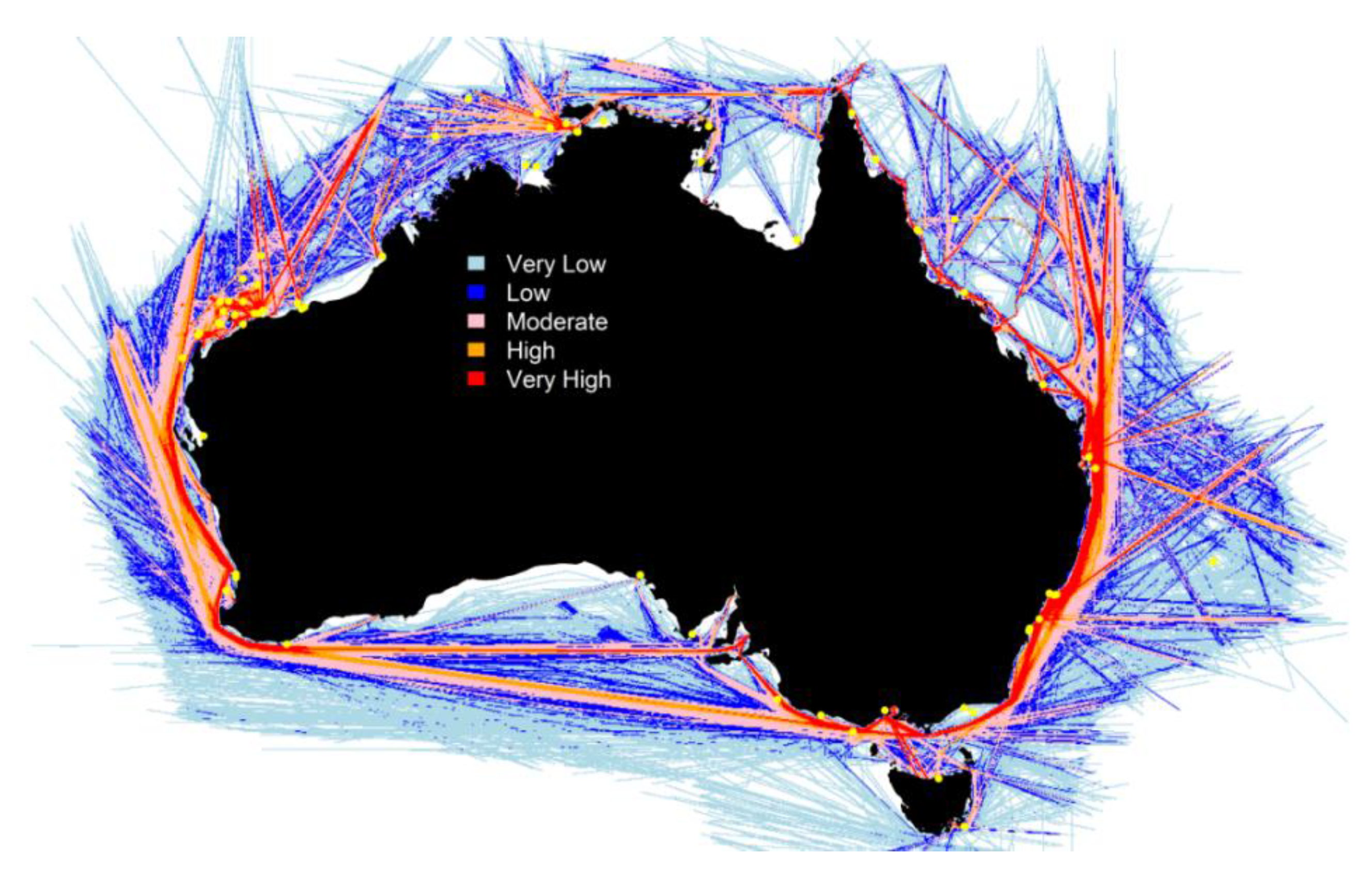
Since spatial visualization of estimates and predictions are important for policy makers in order to understand the magnitude and location of change of risk exposure for medium-term or long-term planning aspects, some examples are provided. The results for expected numbers of collisions is visualized spatially with a flexible resolution in Figure 2 and is compared with observed incidents. The expected numbers were calculated for each grid based on the safety quality of the ships that travelled in this area and the vessel traffic density, which determined the ship-specific risk exposure.
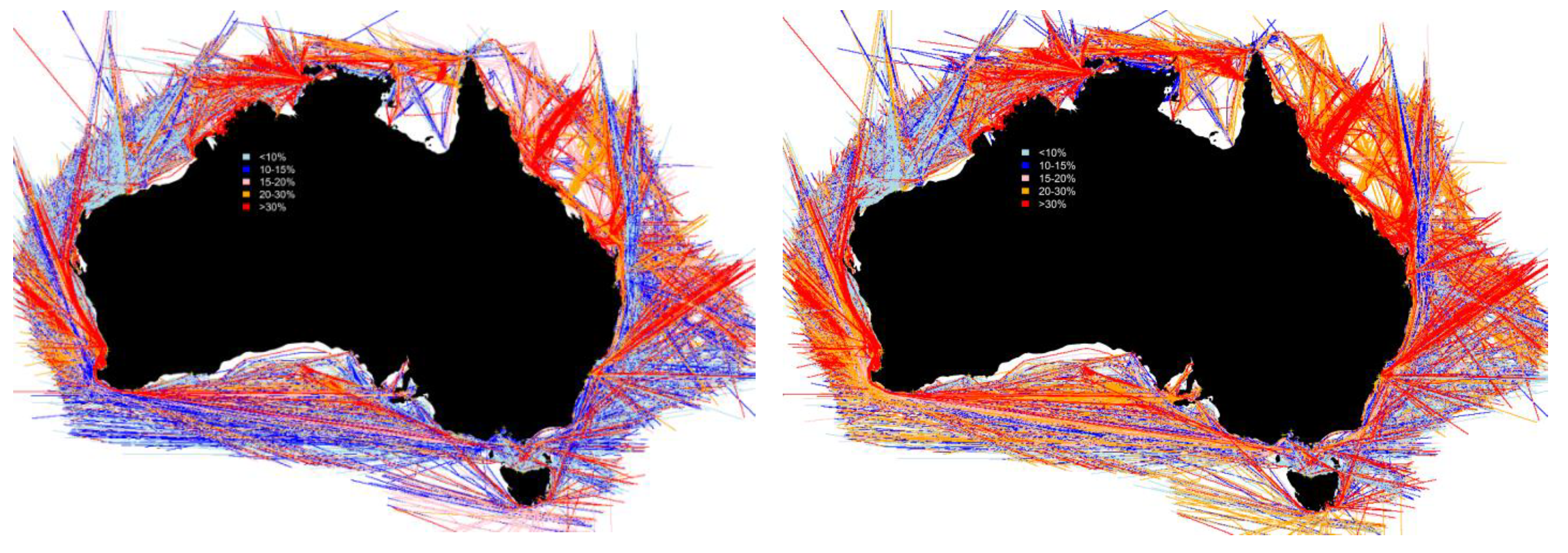
The same type of figure can be provided to visualize change in risk exposure compared to the baseline once suitable spatial correction factors have been implemented, as shown in Figure 3. It can then help us to visualize how risk is spatially distributed and demonstrate the effect of risk control options to mitigate (e.g., Pilotage, VTS, navigational aids, traffic separations, etc.) risk. An example for change in traffic and risk exposure is provided in Figure 3 for the year 2020 and based on a ‘business as usual’ economic development. Ideally, various scenarios reflecting different states of the economy (e.g., bad economy, good economy, etc.) and associated ship arrivals can be applied in the future to see how these changes will affect risk exposure over time. The results can then be used as a basis for sensitivity analysis by running prediction scenarios with different combinations of risk control options. At this stage, spatial correction factors for collisions and groundings are not yet applied for micro-level application.
The categories used in Figure 2 and Figure 3 to classify the risk levels are very low to very high. The thresholds were based on providing a roughly equal number of grid areas for the ‘moderate’, ‘high’, and ‘very high’ categories. All of the remaining grid areas defining the study area were then allocated to very low and low risk. The expected numbers of events appear very low since the associated area size (of a grid) is also very small (~3 nm2). These maps provide an indication of hot spots across a large area such as the whole Australian EEZ since it provides the visualization of the risk areas in addition to calculated figures, such as expected numbers of incidents.
Table 2 also presents a comparison of an expected number of incidents to observed events recorded during a recent period (2006–2010) within the EEZ. These results were based on 38.3 million of nm travelled and risk profiles of almost 7000 individual ships. Observed incidents were not accurate and were, therefore, treated with caution due to the quality issues associated with incident data mentioned earlier. Around 50% of the observations did not have coordinates (lat/long). Despite these difficulties, it is, nevertheless, interesting to make informal comparisons against estimates based on historical incident data. These estimates indicate that the base case scenario is about 5% higher (for drift groundings) than what historical incident data might suggest and up to around 50% to 80% higher powered groundings and collisions.
4. Discussion and Conclusions
The proposed strategic planning tool based on a multi-layered risk estimation framework provides a relatively straight forward approach to maritime risk assessment at the macro level with the possibility to downscale to the micro level by integrating a spatial correction factor. Its main purpose is to provide maritime administrations and coastal states with the means to run prediction scenarios for medium to long term planning aspects in order to allocate assets more effectively. The multi-layered approach can also be adopted for the daily or short-term operational aspect where layers can be combined to create an automated monitoring and alert system to enhance traffic monitoring. This will help coastal states to know as early as possible if a potentially dangerous situation is occurring and intervene to prevent incidents from happening in the first place.
The major difference compared to other approaches in risk assessment for strategic planning is that total risk exposure is divided into layers at the grid level, which can be treated individually or in a combined format. As such, the proposed approach allows the combination of the risk layers with a flexible spatial resolution. One of its main advantages is that it starts at the ship level by capturing safety qualities of ships that trade in a specific area and which can, therefore, reflect how risk will be heterogenous across ships as well as areas.
Several extensions of this application include: (1) to improve estimation of risk at different spatial scales, (2) to assess risk over time, and to (3) predict risk in the future given risk control scenarios and, lastly, (4) to use a combination of the risk layers to create an automated surveillance and alert system to enhance incident prevention. Another possible extension is to add a metric that quantifies potential incident consequences, e.g., the monetary value at risk, which can be estimated at the ship level and aggregated across spatial areas. This would allow improved cost benefit analysis against capital expenditures for asset allocation relevant for strategic planning. The key component for all uses is ship traffic whether it bein real-time or for longer-term traffic predictions. In order to understand risk exposure, the magnitude and location of change in traffic needs to be examined so that change in risk exposure can be monitored over time.
Several areas for future research are identified to extend the framework for its use at the micro level. To increase accuracy in areas where this is most relevant, a location specific weighting factor (referred to here as a spatial rate ratio) should be developed and integrated into the routine as a separate layer. This could be based on, for instance, historical candidates or it could be derived by a proxy variable that can describe traffic geometry such as, for instance, COG (course over ground), the average angle between passing ships, or another suitable proxy.
The current prediction routine still relies on the assumed temporal relationship of the average number of collision encounters being proportional to the number of nm travelled squared, which is widely used in maritime risk assessments for collisions based primarily on the geographic approach. The temporal relationship between changes in traffic and risk exposure may be more complex and might also have a seasonal component and this assumption should be tested.
For strategic planning purposes, risk can (whether they are expected numbers of incidents or monetary value at risk), in theory, be calculated for each of the main shipping routes in the future or for areas of interest to a maritime administration. The most important layer extensions to the framework presented in this case are, therefore, associated with location-specific risk parameters such as risk control options or underlying environmental conditions (wind, waves, and currents) or coastal sensitivities to oil pollution. Another layer that could improve risk prediction for all endpoints is the creation of an available sea-room layer, which quantifies distance to a hazard at the horizontal and vertical level. A logical extension of endpoints would be to add oil pollution and to distinguish between the amount of oil on water and on the coast. While the amount of oil is of interest with respect to strategic planning of oil pollution response assets, the monetary value at risk can provide an indication of damage costs associated with oil pollution, and will enable quantifying of all damages to the marine ecology. Since it is not possible to quantify damages to the marine ecology without a large degree of uncertainty, an alternative way to add this part is via a GIS knowledge layer that quantifies coastal sensitivities to oil pollution at a grid level using qualitative methods such as expert elicitation described earlier.
Lastly, another application of the framework, which is also heavily based on traffic, is to add a routine to estimate air pollution from shipping. To determine hazards, this would have to be coupled with chemical transport modelling and impact assessment on humans and the environment. The framework presented in this case could help address questions involving future scenarios of air pollution from shipping by combining data on pollutant inventories with traffic projections.
One problem with current approaches in maritime risk assessment is that the decision maker is led to believe that the results are definitive and in no way uncertain. The general concept of uncertainty of risk assessment is well established in the literature (Hayes [24]) including the various types of uncertainties. The majority of approaches to maritime risk assessment do not attempt to quantify uncertainty (Merrick and van Dorp [17], Eide et al. [9]). Furthermore, in the few cases where uncertainty intervals are provided, authors take great care to acknowledge the wide range of sources and assumptions and highlight that complete quantification of uncertainty is not possible.
Uncertainties arise from input data, parameter estimates, as along with simplifications and assumptions used in the modelling approach. If qualitative methods are used based on subjective judgement, additional challenges arise, which is mostly relevant for estimating the effects of risk control options (RCO’s) and sensitivities to oil pollution. These could be due to different perceptions, beliefs, and experiences and cognitive biases (Pidgeon et al. [25], Rohrmann [26], Kahneman & Tversky [27], and Fischhoff et al. [28]). In order to handle uncertainty within the general framework proposed in this scenario, uncertainty arising from each source would first need to be considered separately. Several sources of uncertainty that should be considered under the framework presented earlier are described below.
Describing current traffic activity within major regions is of interest to maritime administrations in an operational context as well as for longer-term planning purposes. The risk assessment presented in this scenario is based on one year of AIS data. The next step that would be reasonably straight forward is to apply the method to a longer time series of AIS data in order to gain a better understanding of spatial-temporal variations in traffic behavior. This could be undertaken at a relatively fine geographical mesh level and then be aggregated up to any area of interest. It is unlikely there would be a marked variation in total distance travelled yearly but would be useful to examine variation at the sub-regional level (or for major routes) and/or specific subgroups of the vessel types.
Ship-specific risk probabilities used in this framework are estimated based on a combined dataset consisting of global incident data and global world fleet data based on Knapp [16,20] using statistical models. A related matter concerns the assumption being made when making extrapolations into the future. Logically, it is likely that risk profiles will also change over time. Not only because composition of the vessel cohort will change but also because underlying risk for vessels with the same ship particulars may be different in five or 10 years from what it is today. For example, in the case of collision incidents, risk for a given vessel depends not only on its own safety quality but also interaction with other vessels where the density will clearly vary over time as well as change in the legislative framework. The conventional rule of “change in risk of collision is proportional to the square of change in traffic” has been adopted in this case. However, there is uncertainty in this assumption and testing this relationship is left as a topic for future research.
Changes in the legislative framework might be difficult to anticipate but will influence safety standards for future vessels over and above what might be predicted by the incident models currently available. For example, even though we may be able to forecast what the composition of the vessel fleet may look like for a particular region based on anticipated changes in trade. Those vessels may have somewhat different safety standards. The tendency for most ship types is also an increase in ship size. This is the reason we can only provide predictions of what risk may be in the future by applying our incident models to a given counterfactual traffic scenario assuming that all else is constant. This may be an area that can be further investigated since new risk factors become relevant, e.g., due to changes in the size of vessels and associated safety qualities. Lastly, forecasting future traffic is itself inherently uncertain.
Furthermore, uncertainties are associated with numerical models that describe the physical processes of how the combined forces of wind, waves, and currents act upon the hull of drifting vessels or how oil spreads across water. Input data to model metocean data present uncertainties in their own rights.
Uncertainty intervals for incident rates can be derived directly from historical incident data. Note that this is not the same as quantifying the uncertainty inherent in modelling the underlying system and does not directly address the questions raised above. Historical data on maritime incidents are of poor quality, usually under-reported, and will contain substantial data errors. Global incident data used for this work was compiled from four different data sources (IMO, IHS Markit, LLIS, and the Australian Maritime Safety Authority) reflecting the challenges when basing assessments on the incident data directly.
A comprehensive uncertainty analysis that addresses all of the issues discussed in this section cannot be carried out at this stage. Information and data required to quantify the relevant uncertainties is not yet available. Computer simulations involving different components of the maritime system could (in principle) be carried out, which would allow assessment of the uncertainty across the system including those individual components listed above.
It is important to consider that risk assessment should allow for multiple approaches since each one will have its own strengths and limitations and, therefore, facilitate addressing different questions of interest for a maritime operation such as operational real-time monitoring of vessel traffic or medium-term or longer-term strategic planning. Different approaches may be complementary, e.g., when a micro-level (mechanistic) model provides a better approach to quantify the effect of an intervention in a specific area while macro-level models allow real time applications for larger areas or strategic planning exercises.
Author Contributions
S.K. devised the original ideal and supervised the project. S.V.H. and S.K. developed the theoretical concepts and S.V.H. performed the computations. Both authors discussed the results and wrote the manuscript.
Funding
The Australian Maritime Safety Authority funded this research.
Acknowledgments
The authors wish to thank the Australian Maritime Safety Authority, IHS-Markit, LLI, and IMO for providing the necessary incident, fleet, traffic data, and arrival data.
Conflicts of Interest
The authors declare no conflict of interest.
Appendix A. Logit Models to Estimate Safety Qualities of Vessels
The underlying sample data is a combination of ship particular data of the commercial world fleet, historical inspection outcomes, and past ship incident data for the period from January 2006 to December 2010. Global incident information was combined from four different sources, and duplicates were eliminated. The remaining incidents were manually reclassified, according to IMO definitions [21], for seriousness, which are very serious (including total loss), serious, and less serious incidents. Besides manual reclassification per seriousness, incident initial events were identified when possible, which forms the basis of the models. This allows a better distinction between incident initial events and consequences. The following model types were estimated in Table A1.

Table A1.
Model types.
| Model Type | Use |
|---|---|
| Collisions—very serious and serious | Macro level |
| Powered groundings—very serious and serious | Macro level |
| Drift groundings—very serious and serious | Macro level |
| Drift candidates—irrespective of seriousness | Micro level |
The initial variables of all models and their respective groupings were selected based on Knapp [8,13]. The explanatory variables included in the models are discussed below.
- Ship type, age, and size (GRT) at the time of incident;
- Classification society, flag;
- Country where the vessel was built grouped into four groups, as suggested by AMSA surveyors, and interaction effects with age groups (0–2 and above 14 years represent high age risk, while 3–14 years represent low age risk);
- DoC company and group beneficial owner country of location;
- Number of deficiencies and incidents within 360 days prior to the incident;
- Changes of ship particulars overtime, such as flag changes, ownership changes, DoC company changes, class changes, and class withdrawals (within three years and within five years).
The base model used to estimate the models is the binary logistic model. Let xi contain the explanatory factors such as age, size, flag, classification society, and owner. Then the logit model postulates that P (yi = 1|xi) = F (xiβ), where the weights β consist of a vector of unknown parameters and F is a cumulative distribution function (CDF). A popular choice is the CDF of the logistic distribution, which gives the well-known logit model. This model states the following.
where:
- xiβ is a weighted average of all explanatory variables mentioned before. The probabilities are estimated at the individual ship level (i). The coefficients are estimated by a quasi-maximum likelihood to allow for possible mis-specification of the assumed logistic CDF.
Appendix B. Voyage Database and AIS Data Processing
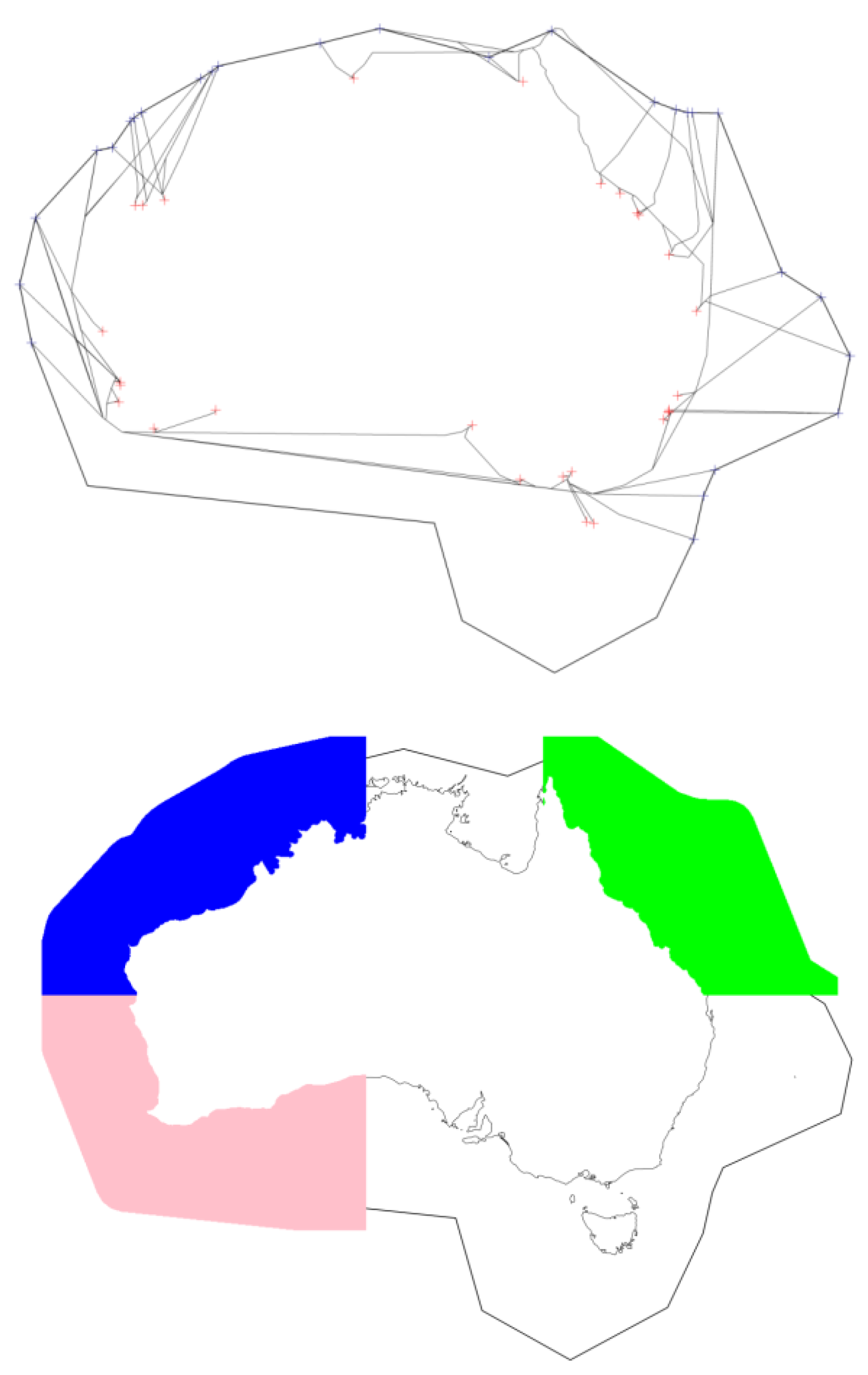
For the purpose of the pilot, one year of satellite and terrestrial AIS data, and AMSA’s RouteNet (Figure A1) was used to generate a voyage database. The purpose of establishing a voyage database is to facilitate generating a counterfactual traffic density based on an alternative scenario, e.g., traffic flow, pattern, and vessel composition in the future (e.g., 2020 and 2025).
Each ship track in the voyage database is classified according to its ship type and voyage description, i.e., origin and destination along with additional summary information such as distance travelled, days at sea, etc. A simpler approach to describing traffic flow along the RouteNet was also considered. At a very basic level, one could assume vessels follow routes, as defined on the RouteNet. Implemented in this way, expected traffic volume and pattern under a counterfactual scenario can be extracted by simply applying the full set of port arrival forecasts to the RouteNet and proceeding with the risk assessment. However, in many ways, this would be inadequate since the simplification of reducing traffic movement to a one-dimensional (linear) model, even at an aggregate level, would ignore the fuller spatial aspects of traffic (and risk), which will likely be needed to address particular risk-related questions that arise later.
One such area of interest concerns testing whether abnormal vessel behavior might be assisted with the establishment of a database containing ‘normative’ ship tracks. Furthermore, while, to a large extent, vessels often do follow a prescribed single path from the point of origin to the destination, understanding where and when this does not occur should be a part of any maritime risk assessment.
Figure A1.
AMSA’ RouteNet and sub-regions (blue = NW, pink = SW, and green = GBR).

The voyage database consists of a collection of spatial lines representing the full set of voyages departing/ending in each major port defined on the RouteNet. The corresponding position on the EEZ boundary is also tagged for each voyage that leaves the EEZ region.
Let SLij represent the spatial line that summarizes the complete set of movements for voyage j of ship type i. For every voyage SLij, a record is also created and added to other summary level data to be used as an index to the actual ship track database SL.
For each SLij, the corresponding distance travelled dij together with other high-level summary data, is recorded on the index dataset. For the analyses carried out, each voyage was further disaggregated, according to the portion corresponding to activity within a port area. Although this disaggregation was not required for the current project, several exploratory analyses have been carried out to study aggregate level vessel behavior at the port level, e.g., port level traffic density and inter-arrival times.
The voyage database also captures other details that may be of interest including whether the vessel enters the EEZ region and bypasses major ports. Preliminary findings indicate that this comprises a relatively small proportion of total traffic. However, it is still required for the purpose of the risk assessment.
Each ship track recorded in the voyage database is classified according to the following five categories.
- port2ee: ship track from port to entry/exit (ee) wayward point on the EEZ boundary
- ee2port: ship track from ee to port
- port2port: ship track from port to port
- port: ship track within port
- ee2ee: ship track from ee to ee, i.e., voyage not tagged as arriving at a port defined on the RouteNet
where:
- Vessels can depart and arrive back into the same port in which case they are classified under category #3.
- Travel for some vessels is restricted exclusively to within the port area. In practice, this did happen with a relatively small proportion of the vessels included in sample data provided by AMSA.
- A port arrival was defined as a vessel staying for at least 12 hours within a 36 nautical radius of a major port.
- Passing through an entry/exit (ee) point was defined as an intersection of a ship track anywhere along the EEZ regional boundary. Note that ee intersections were tagged against major ee positions if the vessel crossed within 90 nautical miles and were otherwise tagged as ZZ.
The definition of a journey passing through an entry/exit point (ee) on the RouteNet is somewhat arbitrary. Different distance values were considered and the numbers of voyages appeared to stay reasonably stable for most routes. A number of journeys could not be associated with a route as defined on the RouteNet such as voyages travelling across the EEZ regional boundary but not through waypoint defined on the RouteNet. Again, this does not directly affect risk calculations.
Several algorithms were tested to clean the ship track data and remove anomalies due to problematic AIS data.
- When a gap between successive AIS readings was less than 24 hours during which time the effective speed was greater than 75 knots. An error is identified whereby the calculated effective speed in invalid.
- When a gap between successive AIS readings was greater than 48 hours and 500 nautical miles distance. This occurred mostly outside the EEZ region. Tracing of ship track data is reset for a given voyage to avoid introducing potential errors.
- Single anomalies with invalid lat/lon are identified and removed, e.g., the vessel suddenly jumps to an invalid coordinate, but then immediately returns to the original tracking position. Other cases involving the AIS data show inconsistencies throughout most of the ship track data where it is unclear which route the vessel is on as the positions repeatedly change back and forth between two very different locations.
Designing an optimal set of routines for handling AIS data was beyond the scope of this project. Specifically, tracks considered to be invalid were removed prior to analysis. The total amount of data removed by employing this step was equivalent to removal of approximately 6M nms.
References
- Bijwaard, G.E.; Knapp, S. Analysis of ship life cycles—The impact of economic cycles and ship inspections. Mar. Policy 2009, 33, 350–369. [Google Scholar] [CrossRef]
- Wood, J. Opa 9. Marit. Policy Manag. 1995, 22, 201–208. [Google Scholar] [CrossRef]
- Goulielmos, A.M.; Giziakis, K. Treatment of uncompensated cost of marine accidents in a model of welfare economics. Disaster Prev. Manag. 1998, 7, 183–187. [Google Scholar] [CrossRef]
- Grigalunas, T.A.; Opaluch, J.J. A natural resource damage assessment model for coastal and marine environments. GeoJournal 1988, 16, 315–321. [Google Scholar]
- Grey, C.J. The Cost of Oil Spills from Tankers: An Analysis of IOPC Fund Incidents. In Proceedings of the International Oil Spill Conference, Seattle, WA, USA, 7–12 March 1999; Available online: www.itopf.com/costs.html (accessed on 5 June 2017).
- IMO. Formal Safety Assessment-Consolidated Text of the Guidelines for Formal Safety Assessment for Use in the IMO Rule-Making Process; MSC 83/Inf.2; IMO: London, UK, 14 May 2007. [Google Scholar]
- Hoorn, S.V.; Knapp, S. A multi-layered risk exposure assessment approach for the shipping industry. Transp. Res. Part A Policy Pr. 2015, 78, 21–33. [Google Scholar] [CrossRef] [Green Version]
- Hueffmeier, J.; Berglund, R.; Porthin, M.; Rosqvist, T.; Silvonen, P.; Timonen, M.; Lindberg, U. Dynamic Risk Analysis Tools/Models, WP6-3-01. 2012. Available online: www. efficiensea.org (accessed on 5 June 2017).
- Eide, M.S.; Endresen, Ø.; Breivik, Ø.; Brude, O.W.; Ellingsen, I.H.; Røang, K.; Hauge, J.; Brett, P.O. Prevention of oil spill from shipping by modelling of dynamic risk. Mar. Pollut. Bull. 2007, 54, 1619–1633. [Google Scholar] [CrossRef] [PubMed]
- Det Norske, V. North East Shipping Risk Assessment, Report Prepared for the Australian Maritime Safety Authority, Report Nr 14OFICX-4. 2013.
- BRISK. Project on Sub-Regional Risk of Spill of Oil and Hazardous Substances in the Baltic Sea, Risk Method Note; Danish Admiralty, 2012; Project funded by Danish Admiralty; Available online: http://www.brisk.helcom.fi (accessed on 5 June 2017).
- Hansen, P.H. Working Document, Basic Modelling Principles for Prediction of Collision and Grounding Frequencies; IWRAP II; Technical University of Denmark: Lyngby, Denmark, 2007. [Google Scholar]
- Montewka, J.; Goerlandt, F.; Hanninen, M.; Ylitalo, J.; Seppala, T. Algorithm Development and Documentation, Study of Algorithm Development Using Data Mining, Efficient Sea Project. 2011. Available online: www.efficiensea.org (accessed on 5 June 2017).
- Heij, C.; Knapp, S. Evaluation of safety and environmental risk at individual ship and company level. Transp. Res. Part D Transp. Environ. 2012, 17, 228–236. [Google Scholar] [CrossRef]
- Heij, C.; Bijwaard, G.E.; Knapp, S. Ship inspection strategies: Effects on maritime safety and environmental protection. Transp. Res. Part D Transp. Environ. 2011, 16, 42–48. [Google Scholar] [CrossRef] [Green Version]
- Knapp, S. The Econometrics of Maritime Safety—Recommendations to Improve Safety at Sea. Ph.D. Thesis, Erasmus University Rotterdam, Rotterdam, The Netherland, 2006. [Google Scholar]
- Merrick, J.R.W.; van Dorp, R. Speaking the Truth in Maritime Risk Assessment, Risk Analysis. Risk Anal. 2006, 26, 223–237. [Google Scholar] [CrossRef] [PubMed]
- Goerlandt, F.; Stahlberg, K. Comparative Study of Input Models for Collision Risk Evaluation, WP6-2-04. 2011. Available online: www.efficiensea.org (accessed on 5 June 2017).
- Knapp, S. Integrated Risk Estimation Methodology and Implementation Aspects (Main Report AMSA), Reference Nr. TRIM 2010/860, 2011-1a (Main Report AMSA). 2011.
- IMO. Reports on Marine Casualties and Incidents, Revised Harmonized Reporting PROCEDURES, Adopted 14th December 2000; MSC/Circ. 953, MEPC/Circ. 372; IMO: London, UK, 2000. [Google Scholar]
- Knapp, S.; Heij, C. Evaluation of total risk exposure and insurance premiums in the maritime industry. Transp. Res. Part D Transp. Environ. 2017, 54, 321–334. [Google Scholar] [CrossRef] [Green Version]
- Carey, J.M.; Knapp, S.; Irving, P. Assessing Ecological Sensitivities of Marine Assets to Oil Spill by Means of Expert Knowledge. 2014. Available online: http://repub.eur.nl/pub/51749 (accessed on 5 June 2017).
- Buhaug, Ø.; Corbett, J.J.; Endresen, Ø.; Eyring, V.; Faber, J.; Hanayama, S.; Lee, D.S.; Lee, D.; Lindstad, H.; Markowska, A.Z.; et al. Second IMO GHG Study 2009; International Maritime Organization (IMO): London, UK, April 2009. [Google Scholar]
- Hayes, K.R. Uncertainty and Uncertainty Analysis Methods; ACERA Report Number: EP102467; Australian Centre of Excellence for Risk Analysis: Melbourne, Australia, 2011. [Google Scholar]
- Pidgeon, N.; Hood, C.; Jones, C.; Turner, B.; Gibson, R. Risk Perception, Risk Analysis, Perception and Management; Report of the Royal Society Study Group; The Royal Society: London, UK, 1992. [Google Scholar]
- Rohrmann, B. Ris perception of different societal groups: Australian findings and cross-national comparisons. Aust. J. Psychol. 1994, 46, 150–163. [Google Scholar] [CrossRef]
- Kahneman, D.; Tversky, A. Choices, values, and frames. Am. Psychol. 1984, 39, 341–350. [Google Scholar] [CrossRef]
- Fischoff, B.; Slovia, P.; Lichtenstein, S. Knowning with certainty: The appropriateness of extreme confidence. J. Exp. Psychol. Hum. Percept. Perform. 1977, 3, 552–564. [Google Scholar] [CrossRef]
Figure 1.
Generic end user application aspects of the strategic planning tool.

Figure 2.
Observed collisions (any seriousness) during 1995 to June 2013 overlaid (as yellow circles) onto the risk assessment for collisions (very serious and serious) in the Australian EEZ.
Figure 2.
Observed collisions (any seriousness) during 1995 to June 2013 overlaid (as yellow circles) onto the risk assessment for collisions (very serious and serious) in the Australian EEZ.

Figure 3.
Change in risk exposure for powered groundings in 2020 (left) and 2025 (right) compared.

Table 1.
Summary of data, data sources, and time frames used.
| Data | Time Frame | Use of Data |
|---|---|---|
| Vessel positions Source: 5-minute down-sampled AIS data from AMSA | 01/01/2014 to 31/12/2014, pre-formatted, cleaned data, linked with ship specific incident type probabilities | Risk estimation routine Calibration factors |
| Global INCIDENT data Source: AMSA, IHS, IMO, LLIS | 01/01/2006 to 31/12/2010 19,740 observations, data compiled based on four sources | Logit models Model validation |
| Regional incident data Source: AMSA | 02/01/1995 to 01/06/2013, 14,428 observations (pre-formatted, cleaned data) | Model validation |
| World fleet data at SHIP level Source: IHS-Markit | 2006 to 2010 and 2012 | Logit models Ship type classifications Calibration factors |
| Nautical miles TRAVELLED Source: IMO, LLIS | 2007, 2013 | Calibration factors |
| Arrival forecasts Source: AMSA Based on a Study from Bramer Seascope | Number of arrivals by ship type for 2020 to 2025 for all major ports in Australia | Input data into the traffic density projections and associated risk exposure estimates |
Note: AMSA = Australian Maritime Safety Authority, IHS = IHS Markit, IMO = International Maritime Organization, LLIS = Lloyds List Intelligence, DHI = Danish Hydraulic Institute, BOM = Australian Bureau of Meteorology, CSIRO = Commonwealth Scientific and Industrial Research Organization.
Table 2.
Expected numbers of incidents by regions and year (base case year = 2014).
| Results by Year | Incident Type (Very Serious and Serious) | ||||
|---|---|---|---|---|---|
| Collisions | Powered Groundings | Drift Groundings | Total | ||
| North West (NW) | 2011 | 0.50 | 0.64 | 0.97 | 2.10 |
| 2014 | 0.70 | 0.74 | 1.10 | 2.55 | |
| 2020 | 1.04 | 0.91 | 1.39 | 3.34 | |
| 2025 | 1.04 | 0.92 | 1.41 | 3.37 | |
| South West (SW) | 2011 | 0.37 | 0.35 | 0.56 | 1.28 |
| 2014 | 0.42 | 0.34 | 0.51 | 1.28 | |
| 2020 | 0.82 | 0.53 | 0.91 | 2.26 | |
| 2025 | 0.86 | 0.55 | 0.95 | 2.37 | |
| Australian EEZ | 2011 | 2.69 | 2.62 | 4.17 | 9.47 |
| 2014 | 3.31 | 3.01 | 4.87 | 11.20 | |
| 2020 | 5.31 | 3.87 | 6.47 | 15.64 | |
| 2025 | 5.73 | 4.05 | 6.90 | 16.69 | |
| GBR (no RCO’s) | 2011 | 0.66 | 0.64 | 0.96 | 2.26 |
| 2014 | 0.85 | 0.74 | 1.16 | 2.75 | |
| 2020 | 1.54 | 0.99 | 1.53 | 4.06 | |
| 2025 | 1.84 | 1.08 | 1.69 | 4.61 | |
| GBR (with RCO’s) | 2011 | 0.41 | 0.34 | 0.63 | 1.38 |
| 2014 | 0.52 | 0.39 | 0.76 | 1.68 | |
| 2020 | 0.90 | 0.51 | 0.98 | 2.39 | |
| 2025 | 1.08 | 0.56 | 1.09 | 2.72 | |
| Observed (with all RCO’s) | 1.80 | 2.00 | 4.60 | 8.40 | |
| Expected (base case scenario) | 3.31 | 3.01 | 4.87 | 11.20 | |
Notes: calculations are restricted to AIS class ‘A’ vessels, EEZ = Exclusive Economic Zone of Australia, RCO = risk control options, unknown ship types were removed from calculations, observed incident data within the EEZ reflect any RCOs that were in operation during that period.
© 2019 by the authors. Licensee MDPI, Basel, Switzerland. This article is an open access article distributed under the terms and conditions of the Creative Commons Attribution (CC BY) license (http://creativecommons.org/licenses/by/4.0/).
Share and Cite
MDPI and ACS Style
Vander Hoorn, S.; Knapp, S. Predicting Traffic and Risk Exposure in the Maritime Industry. Safety 2019, 5, 42. https://0-doi-org.brum.beds.ac.uk/10.3390/safety5030042
AMA Style
Vander Hoorn S, Knapp S. Predicting Traffic and Risk Exposure in the Maritime Industry. Safety. 2019; 5(3):42. https://0-doi-org.brum.beds.ac.uk/10.3390/safety5030042
Chicago/Turabian StyleVander Hoorn, Stephen, and Sabine Knapp. 2019. "Predicting Traffic and Risk Exposure in the Maritime Industry" Safety 5, no. 3: 42. https://0-doi-org.brum.beds.ac.uk/10.3390/safety5030042
Note that from the first issue of 2016, this journal uses article numbers instead of page numbers. See further details here.