
Accidental Combustion Phenomena at Cryogenic Conditions


Department of Civil, Chemical, Environmental, and Materials Engineering—DICAM, Alma Mater Studiorum—University of Bologna, 40126 Bologna, Italy
*
Author to whom correspondence should be addressed.
Safety 2021, 7(4), 67; https://0-doi-org.brum.beds.ac.uk/10.3390/safety7040067
Submission received: 20 July 2021
/
Revised: 15 September 2021
/
Accepted: 23 September 2021
/
Published: 2 October 2021
Abstract
:The presented state of the art can be intended as an overview of the current understandings and the remaining challenges on the phenomenological aspects involving systems operating at ultra-low temperature, which typically characterize the cryogenic fuels, i.e., liquefied natural gas and liquefied hydrogen. To this aim, thermodynamic, kinetic, and technological aspects were included and integrated. Either experimental or numerical techniques currently available for the evaluation of safety parameters and the overall reactivity of systems at cryogenic temperatures were discussed. The main advantages and disadvantages of different alternatives were compared. Theoretical background and suitable models were reported given possible implementation to the analyzed conditions. Attention was paid to models describing peculiar phenomena mainly relevant at cryogenic temperatures (e.g., para-to-ortho transformation and thermal stratification in case of accidental release) as well as critical aspects involving standard phenomena (e.g., ultra-low temperature combustion and evaporation rate).
1. Introduction
Storage and transportation of light gases found economic advantages in ultra-low temperature and low to mid- pressures, because of the elevated density. This aspect is of particular interest for methane and hydrogen, where a decrease in temperature up to cryogenic conditions can lead to liquefaction, with large benefits gained with the elevated volumetric energy density [1]. Besides, the limited impacts on the environment related to the combustion of low-carbon or zero-carbon cryogenic fuels make them convenient in a wider sense [2]. The introduction of ultra-low temperature (T < 223 K) has, however, posed several concerns related to safety aspects. These fears are based on the limited awareness and lack of comprehensive databases and models suitable for the characterization of the chemical and physical behavior of fuels in non-ambient conditions. These limitations can be attributed to the non-fundamentals basis of the experimental systems [3] and promote the development of alternative approaches and techniques. Furthermore, peculiar phenomena playing a significant role only at ultra-low temperatures exist. A clear example is the case of the electronic configurations of hydrogen, characterized by differences in thermodynamic properties [4] and equilibrium composition strongly dependent on the temperature only if lower than 230 K [5]. More specifically, properties for pure ortho hydrogen (o-H2), pure para hydrogen (p-H2), and normal hydrogen (i.e., a mixture of 75% o-H2 + 25% p-H2) (n-H2) cases are significantly different. Hence, distinguishing these configurations is essential for low-temperature systems only. During the liquefaction, catalysts are required to hasten the conversion from the equilibrium composition at room temperature (namely normal hydrogen) to the most stable composition at boiling temperature (almost pure parahydrogen) [1]. In this perspective, some preliminary echoes on the eccentricity of the electronic structure of the hydrogen atoms are provided. Following Pauli’s exclusion principle, the total wave function for hydrogen molecule and wave function in the proton coordinates are antisymmetric [6]. Hence, only antisymmetric nuclear spin and symmetric nuclear rotation (i.e., para-hydrogen) or symmetric nuclear spin and antisymmetric nuclear rotation (i.e., ortho-hydrogen) configurations are possible [7]. A schematic representation of the alternative configurations is provided in Figure 1, where the relative positions and rotations of electrons (E) and protons (P) are represented.
The reversible transformation from para to ortho hydrogen is accompanied by a significant heat release/absorption (up to 708 kJ/kg), thus higher than the hydrogen latent heat (hfg, about 445 kJ/kg) [9]. Hence, it has the potential to play a significant role in temperature distribution in liquefaction processes. Also, variation in temperature profile affects the hydrogen density, thus its dispersion in the atmosphere. However, considering that regardless of the temperature hydrogen vapors are lighter than air, temperature differences should have a limited impact on the size of the area where flammable mixtures can be seen for a given height. However, it can create localized pockets characterized by a higher concentration of fuel. In this light, the implication of para-ortho transformation should be accounted for, especially to describe storage systems in the RPT scenarios. To this aim, accurate estimations of the thermodynamic properties of both hydrogen configurations are an essential step toward meaningful results. Considering the extreme conditions required (i.e., a temperature close to 20 K), high uncertainties could be expected for experimental measurements and strong non-ideal may affect the estimation quality of current models. For these reasons, a comparison of the results obtained by both approaches should be done to corroborate the thermodynamic data and, thus, the analysis relying on them. Several studies have addressed this issue experimentally throughout the last century [10,11,12], building a consistent database for the evaluation of para- and ortho- hydrogen properties. However, numerical models are not available for the estimation of these parameters. Considering the complete theoretical basis, quantum mechanics have the potential to cover this gap of knowledge and supply precise estimations. Besides, its accuracy can be tested by comparing the estimations with the experimental data available.
The following sections will discuss the current understandings and theoretical knowledge on phenomena ruling at ultra-low temperature conditions, including the available techniques suitable for the evaluation of safety parameters. More specifically, this review will analye the following:
- -
- Laminar burning velocity
- -
- Flammability limits
- -
- Ignition (initiation reactions, ignition delay time)
- -
- Mass burning rate
- -
- Evaporation rate
Except for the evaporation rate and mass burning rate, all these parameters are essential for the definition of the safety of cryogenic fuels from the vapor perspective, for any possible scenarios resulting from an accidental release. On the other hand, due to the specific characteristics of cryogenic fuels, evaporation at ambient temperature and pressure (for the case of accidental release without an ignition source) and overall burning rate (for the case of accidental release with an ignition source) are important if the liquid perspective is included in the analyses. Indeed, after an initial, localized and short phase where flash can be observed, the accidental release of cryogenic fuel in an open field can be modeled assuming a liquid pool at atmospheric pressure as a boundary condition. Hence, supercritical behavior can be neglected since the critical pressure can be reached neither by LNG nor by LH2 under the posed conditions. In this light, two separate sections gathering information and models suitable to characterize gaseous and liquid cryogenic systems in terms of safety will be proposed. Based on the defined scope, particular attention will be paid to experimental techniques and models reproducing the physical properties of liquids and thermo-chemical properties of vapors. In addition, a brief overview of the available empirical data and models for the determination of the rate of phase change in subcritical conditions will be presented. Indeed, under the impulse of detailed characterization of accidental release of cryogenic fuels, transcritical and supercritical conditions were not included in this review for the sake of conciseness. However, detailed discussion and insights can be found in the current literature [13].
2. Characterization of Gaseous Systems
Historically, ultra-low temperature systems have been investigated by gradually lowering the operative temperature, thus characterizing the behavior of the gaseous phase at first. In this sense, this section proposes the main parameters and the techniques to determine the thermos-chemical and combustion properties of gaseous mixtures suitable for cryogenic conditions.
2.1. Gaseous Properties
From the numerical perspective, several approaches can be adopted for the evaluation of the thermo-chemical phenomena occurring under conditions of interest for this review [14]. Among the others, apparent and micro-kinetic mechanisms are widespread alternatives. The former usually includes the apparent reactions connecting the initial reactants to the final products and by-products with experimentally derived coefficients, whereas the latter aims to unravel the elemental steps involving unstable intermediates, as well. The main drawback of the micro-kinetic approach lies in the size of the resulting mechanisms (also referred to as a detailed kinetic mechanism). Indeed, the resulting models may consist of hundreds of species and thousands of reactions even for simple systems [15,16], thus prone to error in case of manual editing. Hence, comprehensive models for the description of the chemical behavior of cryogenic fuels and combustion at ultra-low temperature should be generated by using automated tools, driven by the algorithm used to properly select reactions and libraries adopted as sources of the related kinetic coefficients. In this regard, readers are encouraged to refer to the recently published overview of the main techniques applicable to produce kinetic mechanisms [17]. The existing approaches for the automated production of detailed kinetic mechanisms can be classified based on the criteria considered for the selection of species and reactions to be included at each iteration. As a way of example, a rule-based method, as implemented in Genesys [18], or a rate-based method, as implemented in the Reaction Mechanism Generator (RMG) [19], can be mentioned. The former is based on a set of user-defined constraints for the selection of species and reactions to be added, whereas in the latter case species and reactions are included in the mechanisms if the associated fluxes overcome an acceptance criterion. In both cases, many properties are required during the process as input for model generation. The development of accurate micro-kinetic mechanisms describing the chemical behavior at ultra-low temperature represents a key step to gain a general understanding of the systems. Indeed, detailed kinetic mechanisms consist of comprehensive databases either for thermodynamic properties or kinetic parameters. They aim to the reproduction of the elemental steps and decomposition pathways characterizing the investigated species, based on thermodynamics and kinetics aspects [20]. Hence, accurate evaluations of ΔH(T,P) and ΔG(T,P) are essential, at first. To this aim, comprehensive databases can be found in the literature (e.g., [21]). The significance of the quality of data sources for a successful generation of accurate mechanisms has been emphasized [17]. Several approaches can be adopted to gather the information listed in the thermodynamic and kinetic databases, including experiments, correlations, and ab initio calculations. The number of parameters and conditions (e.g., a short average lifetime of analyzed species) to be investigated may discourage the experimental approach, whereas the application of empirical correlations can be limited by the uncertainties associated with them [22], promoting the implementation of the theoretical-based approach [23]. With that being said, extensive libraries including data deriving from experiments and ab initio calculations can be employed [24,25]. The missing information can be inferred employing rate rules and group additivity [26], based on the classification of reactions in appropriate families sorted by the interaction between functional groups. It is worth noting that the optimization (fitting) of some key parameters represents an additional route to produce detailed kinetic mechanisms when experimental data are available. However, in this case, the application of the resulting mechanism should be limited to the range of conditions where tuned parameters were derived, with obvious implications reducing the validity of the mechanisms and the significance of the whole approach. Quantum mechanical calculations are based on the individuation of the most stable conformer or transition state, usually followed by the estimation of the energy associated to the rotation of each routable bonds and frequencies calculations, following the rigid-rotor-harmonic-oscillator (RRHO) method [27]. Eventually, quantities related to the partition function (e.g., heat capacity, enthalpy variation, and entropy) can be calculated starting from the obtained data by solving the molecular Schrodinger equation. A level of theory and a basis set is required to expand the molecular orbitals as a linear combination of atomic orbitals [28]. A comparison of them in terms of computational time and accuracy can be found in the literature [29]. Density functional theory (DFT) is usually utilized for geometry optimization and frequency calculation [30]. However, lower levels, such as the composite methods, are suggested for large systems [31]. G3, G4, CBS-QB3, and CBS-APNO belong to this class and are examples of the level of theory, i.e., the method, commonly adopted to address the numerical combustion chemistry topic [32]. A detailed overview of theoretical approaches, together with an in-depth comparison of assumptions, computational requirements, and accuracy of these methods is out of the scope of this review, but they have been covered by dedicated publications available in the current literature [33,34]. Nevertheless, it should be reported that the CBS-QB3 level of theory is considered as optimized in terms of accuracy for hydrocarbons generated species and computational required [33]. Quite obviously, large sets of basis functions make solutions more accurate but, at the same time, more demanding. Besides, structuring basis sets in the gaussian form make computations easier. Hence, several basis sets were developed with these premises. Among the others, Pople- and Dunning- types are worth mentioning [35]. A generic representation of Pople-type basis sets is A-BCG, where A represents the number of primitive Gaussians considered for each core atomic orbital basis function and it can assume values equal to 3, 4, and 6, B and C are the numbers of bases adopted for valence orbitals, commonly 1, 2, or 3, G indicate the use of Gaussian functions. It can be preceded by the symbol + in the case of diffusion functions and followed by polarization notations. Alternatively, the information reporting information related to the Dunning-type basis sets can be expressed in the compacted form cc-pV, where cc-p indicates correlation-consistent polarized, v valence-only basis sets. Sometimes, this notation can be preceded by aug, representing the augmented version of the indicated basis sets. Further information on the nomenclature and the theoretical principles founding quantum mechanics can be found elsewhere [28,36,37].
The effect of temperature on enthalpy, entropy, and specific heat capacity is commonly expressed in terms of NASA polynomial, i.e., a correlation with 7 coefficients. The variation of temperature is commonly split into two ranges to increase the accuracy concerning the source data, and the low-temperature range usually includes temperature up to 1000 K. However, in most cases data are given for temperature above ambient values, exclusively. In this view, coefficients deriving from ab initio calculations were reported in Table 1, as reported in the literature for most common cryogenic fuels, including different electronic configurations of hydrogen [38,39].
Reported coefficients well reproduce the experimental data available in the current literature [12]. It is worth mentioning that only ab initio calculations can distinguish electronic configurations since most empirical estimators commonly adopted in the literature (e.g., group additivity [26]) are based on the chemical structure and bond energy. These observations confirm the need for accurate calculations for the correct estimation of low-temperature processes.
2.2. Laminar Burning Velocity
Detailed kinetic mechanisms have been historically developed and adopted to characterize chemical phenomena occurring during combustion processes. Besides, most of the analyses available in the current literature have been focused on the evaluation of high temperatures (>1100 K) behavior, whereas only recently the relevance of low-temperature conditions (usually intended as per temperature within 500 K and 900 K) has been pointed out [40]. The high-temperature regime is characterized by unimolecular reactions involving the fuel, favoured by the elevated energy density of the systems, with the formation of unstable intermediate species (radicals). Conversely, the low-temperature chemistry is characterized by hydrogen abstraction by oxygenated radicals (e.g., OH, O2) acting as primary reaction producing fuel radicals, thus laying the foundations for ignition phenomena. For the sake of completeness, in intermediate regime (typically in the range between 900 K and 1100 K) hydrogen abstraction by oxygenated radicals and cracking mechanism compete, together with hydrogen abstraction non-oxygenated radicals [41]. The novelty together with the potentiality of this concept has attracted the researcher’s attention to fill the gap and perform in-depth investigations. However, still, several aspects are unclear or poorly understood [42]. Hence, the utilization of detailed kinetic mechanisms for the characterization of low-temperature oxidation can be beneficial under several aspects. The number of reactions included in kinetic mechanisms, I, has been roughly represented by a linear proportionality to the number of species, K, following the correlation I = 5 K [15]. However, the need of representing wider conditions, together with the inclusion of additional functional groups (e.g., oxygenated species representative of biofuels [43] or hetero atom rings for chemical production [44]) have led to a steeper curve relating these two parameters. Indeed, the implementation of a hierarchical approach makes the detailed kinetic mechanism prone to an undesired increase in size with the increase in molecular weight of the target species. The technological achievements, the increased complexity, and the number of variables involved in the investigated problems have required several practical modifications for the sake of validation. Indeed, the nature and the complexity of typical chemical models promote the addition of an intermediate step, comparing data obtained through simplified experimental apparatus with numerical estimations before the implementation in real systems. To this aim, tailor-made experimental systems have been developed to neglect the influences of non-studied phenomena and reduce the number of unknown parameters. Indeed, laboratory-scale burners are designed to be as much as possible close to a laminar and mono-dimensional regime, to disregard turbulence by chemical and physical phenomena. These simplifications allow for the idealization of experimental systems for the sake of model implementation, making possible a proper comparison of numerical estimations and experimental measurements under comparable conditions. Bearing in mind the conditions under investigation, the laminar burning velocity (Su) is commonly selected as a key parameter for the representation of chemical aspects [15]. Furthermore, Su is commonly used to characterize the severity of accidental scenarios involving reactive systems via simplified and accurate analyses. This approach has the intrinsic advantage of keeping most of the extremely relevant chemical information in a stand-alone parameter for each initial condition, making the validation for several conditions easier. Moreover, these parameters may allow for the estimation of safety parameters [45] and optimal residence time [46]. Further information on this topic will be given in the following paragraphs. Despite the apparent simplicity, several experimental systems have been developed to measure the Su. Among them, the opposed jet method, the closed vessel method, and the flat burner method are commonly used, whereas the utilization of a Bunsen burner is strongly discouraged by the well-known limitations regarding the ambiguous definition of the flame surface [37]. The opposed jet method consists of two counter-flowing jets of fuel or oxidizer, creating stretched flames due to the flue gases flowing to the side of the flame. The strain rate is dependent on the distance from the nozzles, meaning that the unstretched burning velocity can be estimated by repeating the experiments at different strain rates and extrapolating data through logarithmic correlation (Equation (1)), as introduced by Kelley and Law (2009) [47], or linear correlation (Equation (2)), as proposed by Dowdy et al., (1991) [48], to Markstein length (Lb) and stretch rate (k):
where Sb and Sb0 are unstretched and stretched flame velocities, respectively.
The closed vessel method often referred to as a combustion bomb, generates a rotationally symmetric, transient, and stretched flame in a closed vessel, which is often spherical. The burning velocity is obtained by monitoring the pressure profile for time via the extrapolating methods reported for the counterflow flame method.
The flat burner consists of a cylindrical perforated burner plate where steady-state and unstretched flames can be generated, where the assumption of a mono-dimensional flame is commonly accepted since homogeneous inlet conditions are provided [49]. When the stabilization is performed using a heating/cooling fluid controlling the burner plate temperature, this method is referred to as the heat flux method (HFM). The technique, first introduced by de Goey et al., (1993) [50] is based on the balance between the heat loss required for flame stabilization and convective heat flux from the burner surface to the reacting front. In this case, Su has assumed the velocity at which the burner plate shows a constant temperature and is determined by measuring the temperature profile of the plate burner at different gas flow rates and given fuel/oxidant ratio, temperature, and pressure conditions. Alternatively, also the characterization of the flame structure can be considered for validation scope. It is commonly performed via jet stirred reactors [51], where gaseous streams are fed in a spherical reactor by opposed nozzles providing sufficient stir to the mixture, temperature distribution along the reactor is monitored by conveniently located thermocouples, and the composition of the mixture is measured using a movable probe connected to an online FTIR [52]. However, practical requirements have limited the application of this technique to the investigated conditions.
Quite obviously, a complete characterization of chemical behaviour at cryogenic conditions is attractive for light flammable species such as methane and hydrogen. In this sense, a detailed kinetic mechanism suitable for the oxidation of light hydrocarbons at low temperatures allows for the evaluation of the overall reactivity at conditions where data are lacking. Indeed, considering the theoretical approach adopted for the generation of the detailed kinetic mechanism, there is no drawback to its application at low temperature (i.e., temperature lower than 298 K). Hence, Figure 2 and Figure 3 provide an overview of the estimations of laminar burning velocity at a low initial temperature in air for hydrogen and methane, respectively. For the sake of comparison, experimental data were added either for hydrogen [48,53,54,55,56,57,58,59,60,61] or methane [62,63,64,65,66,67,68].
The typical shapes of the laminar burning velocity for the equivalence ratio are not altered by the temperature in both cases. Indeed, an almost linear trend characterizes the lean compositions, whereas parabolic decrease can fairly represent the rich composition case for both fuels. Other than the obvious effect of reducing the overall reactivity, the decrease in initial temperature leads to a shift toward the stoichiometric composition of the equivalence ratio where fundamental laminar burning velocity is observed (φf). This trend is more evident in the hydrogen case, although the investigated values are quite far from the boiling temperature. Considering that initial temperature has a weaker effect on thermal aspects than kinetics, this observation is in line with the assumption of the equality of thermal and kinetic rates at φf. Conversely, the asymptotic values are weakly affected by the initial temperature, confirming the connection between laminar burning velocity and gaseous diffusion at extreme composition. This correlation represents the key hypothesis for the development of the limiting laminar burning velocity theory, commonly adopted for the estimation of the safety parameters, as discussed in the following section.
2.3. Flammability Limits
Several correlations have been developed for the estimation of flammability limits at temperature and pressure differing from the standard conditions where most of the experimental tests are performed. However, these correlations have been developed for temperatures higher than 298 K, without any validations at lower temperatures. Smaller temperatures imply a narrower flammable region because of the reduced reactivity of the mixture. Hence, the safety parameters at a temperature below 298 K have been commonly assumed as equal to the experimental values by a conservative approach. However, the development of a detailed kinetic mechanism suitable for these conditions allows for accurate estimations of these parameters, removing the abovementioned hypothesis. Similarly, the effect of composition on these parameters can be evaluated in a more robust way by using kinetic mechanisms since consecutive and parallel pathways accounting for the pure fuel case are merged. This may be convenient for several industrial applications involving liquefied natural gas (LNG), syngas, or biogas. The accurate determination of safety parameters represents an essential step for safe handling and storage system design and optimization for all the industrial process phases involving gaseous or liquid flammable mixtures. In this regard, the lower flammability limit (LFL) and upper flammability limit (UFL) represent some of the most important safety specifications for flammability hazard assessment. However, both LFL and UFL are strongly affected by unburned gas temperature, pressure, inert concentration and species, apparatus sizing and material, ignition energy, propagation direction, and turbulence. Quite obviously, a first approach is represented by the experimental determination of their values under numerous conditions. To this aim, several systems and procedures have been proposed and utilized in the current literature, as summarized in Table 2.
Among the highlighted aspects, test vessel and ignition criteria represent crucial choices strongly affecting the other experimental rig characteristics. An example of the typical experimental procedure is given by the pioneering study performed by Coward and Jones (1952) [70] reporting a comprehensive database of individual gases and vapors Flammability Limits (FLs) obtained using 50 mm glass tube, 1.5 m long and visual identification, i.e., the mixture was considered flammable only if a flame propagation of at least half tube length occurred. Nevertheless, similar test vessels are still used as proved by the study of Le et al., (2012) [71] on the evaluation of the effect of sub-atmospheric pressure on the hydrogen and light hydrocarbons UFL, where a thermal ignition criterion was applied. A commonly used experimental rig is the spherical vessel with central ignition, where the pressure rises equal to defined values from 1% up to 10% of initial pressure is adopted as ignition criteria [72]. However, in a recent study, Crowl and Jo (2009) [73] have proposed the maximum in the second derivative of the pressure-time curve as a method for the determination of FLs for a gas in a closed spherical vessel. Since the use of the maximum pressure increase as ignition criteria was considered an arbitrary approach leading to not negligible errors especially for hydrogen-containing mixtures.
For the sake of an effective comparison of experimental results, efforts were made to develop standardized test procedures for the determination of FLs, e.g., ASTM E681 [74] and EN 1839 [75], where flask and spherical vessel, cylindrical open and spherical or cylindrical closed vessels, material, dimensions, and ancillary equipment are specified. Additional information and comparison are given in the analysis of EU and US standards for the determination of flammability (or explosion) limits and Minimum Oxygen Concentration (MOC) performed by Molnarne and Schroeder (2017) [76].
A detailed review of FLs experimental data collected at atmospheric conditions from several procedures and empirical equations for more than 200 combustible/air mixtures considered of interest for the prevention of disastrous explosions have been reported by Zabetakis (1999) [77]. Currently, FLs data are required in a wide range of conditions to satisfy the various industrial process operations need and correctly estimate the risk associated with the chemical plants; however, it should be considered that measurements are not always available for all the complex mixture compositions commonly used in industrial applications. For these reasons, an overview of the empirical and theoretical formulas developed so far to estimate the safety parameters as a function of operative conditions are presented in this section. Among the others, critical adiabatic flame temperature (CAFT) [78] and limiting laminar burning velocity [45] theories are worth mentioning. The first alternative assumes that flammability limits can generate a given value of adiabatic flame temperature; i.e., thermal and kinetic aspects are balanced and able to self-sustain a flame [79]. However, although the threshold value should depend on the fuel composition and operative conditions, it is commonly considered within the range of 1200–1350 K [80], leaving a degree of freedom for the estimation of flammability limits. A similar hypothesis was posed by Hertzberg [45], but the balance between thermal and kinetic aspects was scrutinized by using the laminar burning velocity as a monitoring parameter. In this case, a correlation for the evaluation of the effects of operative conditions on the threshold value was provided:
where , , , and represent the gravitational acceleration, effective thermal diffusivity of the mixture, burned, and unburned densities.
For economic reasons, storage in cryogenic conditions may potentially involve either hydrogen, natural gas, or ethylene. Excluding a small number of impurities, natural gas represents the only case where composition can significantly variate. Anyway, methane, ethane, and propane are the most abundant species in purified natural gas. Hence, three alternatives were selected as representative of LNG composition (Table 3).
Hence, the estimations resulting from the application of KiBo were reported for these species and mixtures in the presence of air (Figure 4). Experimental data from the literature were added, when available. Please note that the reported lower temperature differs per fuel following the variation in flashpoint or boiling point of oxygen.
An excellent agreement between experimental and numerical data can be observed at extreme conditions, as well, testifying to the comprehensiveness of the adopted mechanism. As expected, the decrease in temperature makes the flammable regions narrower, regardless of the analysed fuel. However, it is worth mentioning that only the LFL of hydrogen follows a linear trend with temperature, meaning that the assumption of the thermal aspect dominating the reactivity at the lean limit cannot be extended to methane and ethylene at low temperatures. On the other hand, similar trends can be observed once the effect of temperature on UFL is compared. These phenomena can be attributed to the difference in the overall reactivity of the investigated species. More specifically, temperature decrease makes the hypothesis of instantaneous reactions at lean conditions not applicable for fuels having low overall reactivity, exclusively.
2.4. Ignition Phenomena
Regardless of the investigated conditions and reactive systems, reactions can be distinguished between the following classes: (1) initiation; (2) chain branching, (3) chain propagation; (4) chain termination. The fate of the reactive system is determined by the proportion between these classes of reactions. Hence, this paragraph will be dedicated to the description of a generic structure typical of detailed kinetic mechanisms, suitable for 0-dimensional systems, namely for the investigation of pure chemical behavior.
The initiation step is an activated reaction producing more reactive species, e.g., radicals, starting from a stable compound (AB) and an unstable compound (C). This reaction class can be expressed in the generic form:
Typical examples of these reactions are dissociation reactions and hydrogen abstraction. The former indicates a reaction like A = B, whereas in the latter case A usually stands for hydrocarbons chain and is substituted by the symbol R, B represents the hydrogen atom, and C is referred to as abstracting agent. C may represent several species, mostly small radicals. Among the possible abstracting agents, OH, H, O, O2, and HO2 are worth mentioning in combustion applications [20]. The relevance of radicals indicated by C and, thus the ruling decomposition path, is strongly affected by the temperature. Indeed, low-temperature regimes are characterized by an elevated amount of HO2 resulting from the initiation step [87].
Chain branching reactions are characterized by the production of radical(s) starting from unstable intermediates as reactants, increasing the overall number of radicals available and the reactivity of the systems. Hence, the so-called growth phase observable by monitoring the heat release rate of flames can be attributed to this reaction class [88]. On a macroscopic scale, this phase corresponds to the ignition. Assuming this reaction class as a continuation of the initiation step, a generic representation can be expressed as follows in terms of the generic molecules or chemical groups D and E:
The equation above is a general form potentially expressing typical examples of chain branching reactions characterizing OH formation and, thus, combustion application. More specifically, two cases are dominant in a wide range of conditions: (I) A is an oxygen atom, D = E and represents a hydrogen atom, or conversely, (II) A stands for a hydrogen atom, D = E and represents an oxygen atom [56].
Chain propagation reactions are characterized by the same number of radicals on the reactants and product sides. However, a slight decrease in the overall reactivity is commonly attributed to the occurrence of this class of reactions because it tends to consume OH radicals to form less reactive species [89].
Eventually, chain termination reactions considerably reduce the tendency to react to the system. Third bodies, such as reactor walls or inert species, can be involved in partially absorbing the energy of excited species and producing more stable species [90].
It is worth mentioning that the case where only two or more stable species react is neglected in micro-kinetic mechanisms because of the limited rates associated with the interactions between closed-shell species. On the other hand, this class of reactions usually composes empirical-derived mechanisms because of greater simplicity in measuring stable species. This classification can be used to provide indications on the ignition behaviour concerning the initial conditions, under Zeldovich theory [91], by estimating the evolution of the free-radical density () with respect to time (t):
where account for the inverses of the characteristic time of the system; cb and ct stand for chain branching and chain termination, respectively. Indeed, depending on the sign of the brackets a decrease or an increase in free-radical density will be observed, determining the fate of the system.
Undoubtedly, migration from high to low temperatures has a terrific impact on the ruling reaction pathways and, thus on overall reaction rates. Further clarifications and insights corroborating this statement can be gained by analysis of a specific case. In this sense, the case of alkanes combustion may represent a convenient option, because of the large availability of information [92]. The high-temperature mechanisms are characterized by the presence of a pyrolysis path, leading to the formation of aromatics and soot precursors via an increase in the aliphatic chain and hydrogen addition reactions. Besides, two distinct paths can be conducted to high-temperature oxidation. Both follow the CH2O → HCO → CO → CO2 route as the final steps. However, in one case CH2O is produced via alcohol intermediate by hydrogen abstraction reaction followed by double bond formation, whereas in the other case the abstraction site is on the hydrocarbons side. It is well-established that hydrogen abstraction is the ruling primary reaction for alkanes combustion, provided that the initial temperature is below 1200 K [93].
A simplified reaction path representative for ultra-low and low temperatures is reported in Figure 5.
Low-temperature combustion is characterized by having oxygen molecules as dominant abstracting agents, producing the alkyl group (indicated as R in) and hydroperoxy radical (HO2). This phenomenon can be attributed to the reduced availability of small radicals, deriving from dissociation reactions. Indeed, this reaction class is favored by elevated internal energy and momentum, thus hindered by decreases in temperature. The produced alkyl radical may undergo further hydrogen abstraction by oxygen, to form an additional hydroperoxy radical and alkene, or attract an oxygen molecule and produce a peroxyalkyl radical (). The latter is considered being a barrierless reaction [94], justifying the fact that it is dominant at low temperatures. The production of HO2 (as reported for the primary and secondary reactions with O2) represents a peculiarity of low-temperature combustion and characterizes the whole ignition phenomena. Indeed, this radical can be easily involved in chain branching reactions breaking the O-O bond and generating hydrogen atom (H) and hydroxyl radical (OH). The formation of these radicals fastens the reactivity of the system, determining the ignition. On the other hand, more stable compounds, such as alkenes, are produced reducing the overall reactivity. Hence, the relative rates of these branches determine the ignition behaviour at low temperatures, causing the negative temperature coefficient (NTC) behaviour in some cases; i.e., a decrease in the global reactivity determined by an increase in temperature [95]. Other than temperature, the branching ratio is affected by the number of carbon atoms forming the reactants. Indeed, concerted elimination of HO2 forming alkene is neglected for alkyl radicals having more than 4 carbon atoms [96]. Hence, a full understanding of low-temperature combustion mechanisms assumes relevance, especially for light hydrocarbons. Since the scope of this review is to report the main understandings of the combustion mechanisms occurring at low-temperature, a special emphasis will be placed on the reaction paths starting from the . In this light, two major reactions should be highlighted: the disproportionation with other radicals, forming a hydroperoxide (ROOH), and the internal migration of hydrogen atom, resulting in a hydroperoxyalkyl radical (QOOH). Based on the analysis reported by Curran et al., (1998) [96], the latter reaction is dominant when the temperature is above 600 K. Once formed, ROOH decomposes to RO and OH radicals via a degenerate branching step. On the other side, QOOH can be involved in three major paths: the addition of oxygen molecules, decomposition to cyclic ethers, or decomposition to acyclic species. The first option results in peroxyhydroperoxyalkyl radicals (OOQOOH), which reacts as QOOH. The major path leads to the formation of keto hydroperoxides [97]. Additional information on the most relevant reaction paths characterizing high- and low- temperatures can be found in dedicated literature reviews [97,98].
Based on the intrinsic nature of the investigated phenomena, thermal aspects should be combined with thermodynamics and kinetics phenomena, as suggested well-known Semenov theory. This alternative approach is oriented on the evaluation of ignition based on macroscopic and easily measurable parameters. Indeed, the overall power produced by the reaction (Qr) and the amount of power removed by the cooling system/environment (Qe) should be comparable. In complex systems, Qr can be intended as the sum of all the contributes Qr,i of the i-th reaction, as defined in Equation (7):
where V is the volume of reacting mixture, is the heat generated per unit mass of reactant by the reaction i at the temperature T, and is the reaction rate of the reaction i at T. can be defined in the most general form as:
assuming as the convective heat exchange due to mass flow, as the heat losses, as related to the mechanical energy dispersed by moving objects, U is the overall heat transfer coefficient, S the heat exchange surface and Tw the vessel wall (equipment) temperature, which can be correlated to the cooling fluid temperature, if any, or to the ambient temperature. , when present, is converted into viscous friction energy and finally altered into thermal energy. In most cases, it is negligible when compared to the heat released by combustion. The last term accounts for the actual heat exchange between the bulk of the reactants and the equipment system, which is typically the prevalent process in any process. Under these assumptions, an almost linear trend of with T can be expected, thus the comparison of and results in three different alternatives, as reported in Figure 6:
- Curves for produced heat and exchanged heat are secant. The conditions represented by the lower intersection are considered stable because the system can restore the initial conditions in case of moderate and localized variations. In other words, an increase in temperature leads to faster heat removal, with a consequent decrease of the bulk temperature, whereas a decrease in temperature makes heat removal slower than heat production, with a consequent increase of the bulk temperature. In contrast, the conditions representative for the intersection occurring at higher temperatures are considered unstable since any modification in operative temperature is accomplished by positive feedback.
- Curves for produced heat and exchanged heat are tangent. The conditions represented by the intersection behave like the ones corresponding to the intersection occurring at the higher temperature described in the previous case. Hence, they are intended as critical conditions.
- Curve for produced heat and exchanged heat are separated. The absence of intersections between the curves is representative for super-critical conditions, thus to unstable points regardless of the temperature variation.
Given a flammable mixture, the initial occurrence of one or more uncontrolled, exothermic reactions may be triggered by several factors, such as deviation of the real composition from the setpoint, abrupt variation in the operative conditions (even locally), failure or damages in ancillary systems, or by the presence of impurity into the vessel. Regardless of the causes promoting side reactions, the occurrence of undesired exothermic reactions may increase bulk temperature and/or affect the fraction of liquid fuel stored. The former generates positive feedback in gaseous kinetics, whereas the latter produces an abrupt decrease in density in a closed space. Hence, both circumstances cause an increase in pressure, potentially damaging the storage tank.
Based on the discussed models and approaches, a flow diagram that summarizes a possible workflow for the characterization of ignition phenomena using thermo-chemical considerations was produced, in a general perspective, and reported in Figure 7.
3. Characterization of Liquid-Vapor Systems
Once a biphasic system is investigated, the characterization of the chain of events is essential. Indeed, in the case of cryogenic fuels, the amount of vapor available for combustion is related to the net transfer rate between liquid and vapor sub-systems. Subsequently, the geometrical distribution of a flammable cloud determines the ignitability and the overall reactivity (e.g., due to fuel and thermal stratifications), thus the fate of accidental release of cryogenic fuels.
For the sake of accurate analyses, models for the estimation of the density of liquids and vapors, as well as the determination of phase diagrams at cryogenic conditions are essential. Hence, researchers’ attention has been posed to the development of the equation of states (EOS) and experimental apparatus suitable for the investigated conditions. Indeed, the traditional approaches have limited accuracy at ultra-low temperatures, requiring the development of more comprehensive models accounting for a significant role of non-ideal behavior [99]. This issue still represents a significant challenge either for measurements or theoretical derivation [100]. As a way of example, binary mixtures have been only recently tested [101].
Throughout the decades, several real-fluid EOS have been developed or modified [102,103]. Typically, these models can be distinguished by the number of parameters required (e.g., two-parameters, three-parameters). Alternatively, EOS are classified based on the parameter adopted for the formulation, such as Gibbs energy, enthalpy, internal energy, or Helmholtz energy. The latter has the intrinsic advantage to be continuous within the phase boundary and a function of measurable properties. Most EOS quantify the repulsive and attractive forces among molecules and use correction factors depending on the acentric factor and reduced temperature. Among the others, Benedict-Webb-Rubin (BWR), Jacobsen and Stewart (JS), Soave Redlich Kwong (SRK), Peng Robinson (PR), and cubic equations are worth mentioning. In particular, SRK and PR have been widely used for numerical analyses, being a good tradeoff between accuracy and computational efficiency [13]. The comparison of models accuracy in predicting the thermodynamic properties of light gas published by Nasrifar (2010) [104] has indicated that the modification to the SRK equation proposed by Mathias and Copeman (RKMC) leads to increased accuracy.
In this perspective, this section was divided into three subsections gathering some of the available data as well as the widely used approaches and models for the characterization of pool evaporation, the behaviour of non-reactive liquid-vapor systems, and behaviour of reactive liquid-vapor systems, respectively.
3.1. Evaporating Pool
In the case of the accidental release of cryogenic fuel, an evaporating pool is suddenly formed. The presence of ignition sources in the proximity of the releasing point and the substrate where this phenomenon occurs strongly affects the fate of the consequent accidental scenario. In case of immediate ignition, a pool fire scenario is triggered. Eventually, if the ignition is delayed, the formed vapor ignites resulting in flash fire scenarios potentially triggering pool fire, as well. Considering the nature of the described scenarios, the first can be intended as a diffusive flame burning the evaporated fuel in the proximity of the liquid pool, whereas the latter scenario is characterized by thermal and mass stratification. Indeed, vapors produced by LNG are denser than air at first, thus a preliminary phase where LNG can be modelled as dense gas (i.e., it mostly spreads horizontally) occurs. Then, the decrease in density due to the mixing and heat exchange with the environment leads to a subsequent behaviour like neutral and light gases. The combination of these mechanisms produces significant gradients in fuel and temperature distributions. The tendency to act as dense gas has been observed for liquid hydrogen too, by Hansen (2020) [105]. For the sake of safety analyses, the stand-off distance of pool fire is typically calculated based on the incident heat flux on a given position/target, whereas for flash fire distances are estimated through the LFL values [106], thus neglecting the combustion-related phenomena. This assumption may appear an oversimplification once cryogenic conditions are involved. In this perspective, specific insights on the combustion phenomena characterizing liquid-vapor systems will be provided in the following sections.
In the case of release on water, the intimate liquid-liquid interactions may lead to elevated heat transfer coefficients, promoting sudden evaporation. The abrupt change in the state produces a localized variation of specific volume, thus posing the foundations for the generation of overpressures. This phenomenon is called a rapid phase transition (RPT) and represents an additional scenario to be considered for the sake of consequence analyses involving cryogenic storage systems, especially for the case of liquid hydrogen [107]. Additional information on the main approaches adopted for the characterization of these scenarios will be provided in the following.
Undoubtedly, prior evaluation on the pool formation and evaporation represents an essential step for meaningful results and proper characterization of the accidental scenarios involving cryogenic release. In this sense, a generic equation correlating the pool mass per unit area () to time (t) can be expressed as follow:
where the subscripts spill, ev, and dis stand for spilled, evaporated, and dissolved, respectively.
The dissolved term accounts for the fraction of liquid adsorbed by the substrate where the pool is spreading. This contribution can be neglected for cryogenic release regardless of the composition of the spreading surfaces (e.g., either for water or concrete). Hence, the evaporation rate is commonly assumed equal to the spilling rate once the steady-state conditions are achieved. Quite clearly, this approach is unadaptable for different unsteady conditions as e.g., for short instantaneous release and can lead to significant overestimations for the continuous release case. Consequently, the development of robust models accounting for phenomena involved in liquid-gas phase transition is desirable. In this light, the main aspects involving the evaporation of a liquid pool are schematized in Figure 8. For the sake of simplicity, no barriers limiting the pool geometry were assumed, resulting in a cylindrical pool.
Under the assumption of pure liquid, a constant latent heat of vaporization () and boiling temperature can be considered. Hence, the evaporation term can be intended as the sum of the conduction (cond), convection (conv), and radiation (rad) heat fluxes (q)
The radiative heat flux can be neglected in the absence of ignition sources. Besides, due to the major differences between the pool and substrate temperature, the conduction term is usually dominant at first, then, the convective term assumes significance [108]. The conduction term accounts for the heat transferred from the substrate where the pool is formed, thus different models can be used if the release occurs on water or solid. Assuming LNG as pure methane, Conrado and Vesovic [109] applied the following model in the case of release on water:
where is the heat transfer coefficient between water and LNG, T the temperature, and the subscripts w and P represent the water and pool, respectively.
Under the hypothesis of semi-infinite solid at a constant temperature, the model developed by Carslow et al., (1986) [110] can be adopted for the evaluation of conduction term to time t in case of a solid substrate, based on the thermal conductivity , thermal diffusivity , solid substrate temperature ,
The convection term is commonly expressed as the product of the driving force heat transfer coefficient. The former is the difference between room and pool temperatures, whereas the latter can be estimated via several equations correlating the Nusselt number to Reynolds and Prandtl dimensionless number [111,112], the suitable for the investigated layout and turbulence.
Alternatively, a fundamental approach may correlate fluid properties and boundary conditions to the evaporation rate. In this light, it should be considered that this phenomenon can be intended as a non-equilibrium process having a net transport of liquid molecules across a liquid-vapor interface into a gaseous phase [113]. In other words, models for the evaporation rate estimation can be the sum of two different contributes:
- condensation of evaporated molecules in the area surrounding the liquid.
- evaporation of liquid molecules in the atmosphere.
The available fraction of these two states of aggregation is, in the first approximation, regulated by well-known thermodynamic correlations, e.g., the Antoine law. Following this approach, several models have been developed for either cryogenic or non-cryogenic conditions. In both cases, the evaporation rate per unit of liquid surface () can be expressed as a function (f) of the driving force, i.e., the effects of the vapor pressure at the liquid temperature , and a function of thermodynamic properties, transport coefficients, and/or boundary conditions (hx)
Either linear (Equation (14)) or logarithmic (Equation (15)) trends can be used to substitute f
where the subscripts , s, and a represent the liquid surface, saturated conditions, and atmosphere, whereas the symbols P, and are the pressure, ideal gas constant, temperature, and molecular weight, respectively. A comparison with experimental data has demonstrated that the linear trend is more accurate for cryogenic applications [114].
Further distinctions can be done based on the approach adopted for the evaluation of . Indeed, can be intended as an empirical-based coefficient, a function of thermodynamic data, or fluid dynamic properties. The latter case is commonly expressed in terms of dimensionless numbers, such as Reynolds , Schmidt . Examples of correlations for the estimation of were reported in the following Table 4.
It should be noted that some correlations have been specifically developed for cryogenic conditions but in a non-terrestrial environment. These peculiar conditions have led to a neglect of the effect of wind, included by most of the correlations. Since consequence analyses are usually performed under the benchmark stability classes 5D and 2F, referring to a characteristic wind speed of 5 m/s with Pasquill atmospheric stability class D and 2 m/s with Pasquill atmospheric stability class F, respectively, correlations including the effect of wind should be preferred. Besides, the lack of comprehensive databases including data on the evaporation rate of cryogenics, discourage the adoption of fully empirical correlations having unknown relaxation coefficients. Similarly, in the case of accidental release on the water surface, several models can be implemented for the evaluation of the evaporation rate [127]. Besides, the introduction of additional parameters (e.g., water depth and agitation) is necessary to satisfactorily describe the substrate conditions and, thus, the evaporation rate [128]. Furthermore, the significant difference in temperature between the substrate and fuel has the potential to cause the solidification of water. However, theoretical analyses have demonstrated that this phenomenon can be neglected for deep or turbulent water [129]. Regardless of the composition, the immediate formation of a vapor film over the liquid surface can be assumed and, thus, the evaporation rate can be estimated as in Equation (16) [109]
where represents the heat transfer coefficient between substrate and liquid pool, the latent heat of vaporization, the wall temperature, the pool temperature. It should be noted that can be assumed as constant if the substrate is sufficiently larger than the pool and thus heat can effectively disperse the heat. On the other hand, variates unless pure liquids are considered. Eventually, can be estimated by suitable correlations, such as the ones developed by Klimenko [130], reported in terms of dimensionless numbers (Nu = Nusselt, Pr = Prandtl, Ar = Archimede).
in which and are the so-called near unity correction factors, defined by Klimenko in terms of reduced latent heat of vaporization, whereas , k, and l stand for thermal diffusivity, thermal conductivity, and critical wavelength of the instability, respectively. The latter is defined as reported in the following equation:
provided that , , and are surface tension, gravitational acceleration, and density, and the subscript v indicates cryogenic vapor.
3.2. Non-Reactive Liquid-Vapor Systems
Once the evaporation model is carefully selected, computational fluid dynamic (CFD) models can be adopted for the evaluation of near-field aspects involving the vapor phase resulting from an accidental release of cryogenic fuels.
Recalling the events previously defined in this work, either physical or chemical phenomena may show some peculiarities due to the low-temperature conditions. More specifically, based on the thermodynamic properties, vapors may act as dense gas when the temperature is below a given value (e.g., about 200 K for LNG), whereas are lighter than air as the temperature approaches the room value [27,105]. In absence of ignition sources, a visible cloud is commonly generated from the liquid pool. A widespread approach to characterize this scenario is the estimation of the methane distribution along with the distance from the releasing point. Although the transient nature of the investigated system, numerical results are usually presented in a pseudo-steady state form by assuming the most conservative time. Once liquids are released in the atmosphere, a visible cloud is formed immediately. It is related to the condensation of moisture present in the atmosphere caused by the contact between the atmosphere and cold vapor [131]. Hence, the cloud can be characterized either in terms of flammable or visible footprint. The former can be expressed as the maximum distance from the releasing point where LFL is observed (dLFL) [132], while the latter can be defined as the maximum distance where the measured temperature and dew point (Tdew) are equal (dVis) [131]. The Tdew can be calculated by using Bosen’s correlation [133], reported below (Equation (20)).
where H is the relative humidity in % and Ta is the ambient temperature in Celsius, respectively.
The ratio between these factors is defined as the dispersion safety factor (DSF) (Equation (21)).
Wind speed, atmospheric temperature and humidity, pool size, and the material forming the substrate affect either dLFL or dVis. However, differences in the size of these variations make also DSF dependent on these parameters [134].
Alternatively, the transition between film and nucleate boiling regimes may result in an RPT [135]. The distinction between these regimes is made by the critical heat flux (), defined in Equation (22) and used for the evaluation of the evaporation rate m″ev (Equation (23)) [136].
where the coefficient a is equal to 0.16 for the case of hydrogen [137], λ is the latent heat of vaporization, is the liquid density, is the vapor density, g is the gravitational acceleration, r is the pool radius, and is the surface tension. Although, the same symbol is used for the evaporation rate in the absence and presence of ignition, the former should be considerably smaller than the latter because of the absence of heat generated by the combustion process. The characterization of consequences resulting from RPTs goes through the assessment of the maximum overpressure generated. In this sense, the correlation reported in Equation (24) provides a rough estimation of this parameter with respect to pool radius (r), the density of the mixture at the boiling temperature (), molar weight (), and evaporating velocity (vr) [39].
For the sake of consequence analysis in the case of RPT, some empirical-based correlations have been developed, as well [106]. However, most of them neglect the peculiar properties at cryogenic conditions since they have been developed for atmospheric conditions. In this view, methods accounting for the endothermic transformation from para to ortho hydrogen should be preferred [11]. Recently, computational fluid dynamics has been integrated with a detailed kinetic mechanism including theoretical-based thermodynamic properties for the characterization of liquid hydrogen release on water [38]. Based on the releasing rate, two regimes have been distinguished and classified in terms of the generated overpressure.
Because of the robustness of the required infrastructures, most large-scale campaigns have been devoted to the analysis of LNG for the sake of risk assessment of LNG transportation via ship systems. Either experimental or numerical approaches have been adopted to this aim. Nevertheless, small scale data can be found, as well. In this section, a brief overview of the main data and conditions experimentally tested, together with the models considered as more accurate will be reported. Small scale RPT experiments performed by Enger and Hartman (commonly referred to as Shell tests) [138], testing a 0.1 m3 pool composed of a mixture of light alkanes, have proved that RPT does not occur unless methane content is lower than 40% in volume. On the other hand, large-scale tests included in the Coyote test series [139], performed by the Lawrence and Livermore national laboratory (LLNL), have reported RPT for LNG having methane content up to 88% in volume. In this case, several compositions including methane, ethane, and propane, selected as representative of LNG were tested realizing a continuous spill having flowrate within 6–19 m3/min. Under these conditions, only a fraction of tests has reported the RPT. However, either early (i.e., in the proximity and immediately after the spill begin) or delayed (i.e., far from the releasing point and at the end of the spill) RPTs have been observed. The discrepancies between the two experimental campaigns are reported here, indicating that different mechanisms rule the RPT based on the pool size. Differences in water temperature can be considered additional criteria. Indeed, the hypothesis of 290 K as the threshold value of water temperature for RPT occurrence has been accepted [140]. Similarly, the superheat temperature theory has been adopted to correlate this value to the fuel composition. More specifically, it has been assumed that the water temperature should be within the range delimited by the superheat temperature and its 110% [141]. This parameter has been evaluated for several pure species [142] and can be approximated for mixtures based on a mole fraction [143]. Quite obviously, the evaporation rate and vapor composition variate along with the test, because of the differences in the volatility of the involved species. The delayed RPT is attributed to this phenomenon, causing the enrichment of ethane in the LNG pool along the time [135]. Considering the significant differences between the room temperature and LNG boiling temperature, the instantaneous formation of the film boiling regime is commonly assumed, then the RPT is attributed to instabilities leading to local collapses of the vapor layer leading to liquid-liquid contact [144].
Several experimental tests have been performed for the characterization of the LNG dispersion scenario, either on water or on solid surfaces. Among the others, Esso [145], Maplin Sands [146], Burro [147], Coyote [139], and Falcon [148] series are worth mentioning. These campaigns span from a small scale (e.g., approximate pool radius of 5 m) to a large scale (e.g., approximate pool radius of 30 m). Several compositions were tested. Visible plume sizes and maximum distances where lower flammability limits were observed were reported as a function of wind velocity, air humidity, spill rate, and pool size. Dense cloud behaviour has been reported in all tests; i.e., LNG vapor tends to spread on downwind size predominantly, forming a cloud low in height compared to the downwind direction. Vapor density was found to be sensitive to the level of humidity in the surrounding area. A comparison of qualitative and quantitative analyses performed during the Burro series show that the LFL can be detected within the visible cloud even for an extremely low level of humidity (i.e., 5%). Most of the computational fluid dynamic analysis performed so far have evaluated the LNG vapor dispersion by using the k-ε sub-model for turbulence, 2F and 5D as Pasquill stability classes and wind velocity. The effect of pool area and shape, release rate, substrate roughness, presence of obstacles, and atmospheric conditions have been tested, showing an increased relevance of parameters affecting source term when wind flows slowly because gravitational forces are dominant [149].
3.3. Reactive Liquid-Vapor Systems
If an ignition source is present, the accidental release of cryogenic turns into a pool (or tank) fire. In this case, it should be considered that kinetics is strongly affected by the temperature, and low-temperature combustion affects the ruling pathways toward the complete and partial oxidations. Hence, the implementation of detailed kinetic mechanisms in CFD has the potential to solve both issues, because of the exhaustive thermodynamic database included in them. However, the computational power available strongly limits the feasibility of this approach. On the other hand, the implementation in a reduced form of kinetic mechanisms in CFD for an accurate representation of real systems has been indicated as a promising technique in several industrial fields [150]. This approach lays the foundation on the individuation of the most representative pathways and species for the investigated conditions. Indeed, reducing the size with negligible effects on accuracy means narrow the operative conditions accounted for in the model. Hence, the most representative values should be individuated by carefully evaluating the investigated scenarios. To this aim, sensitivity analysis and reaction path analysis are commonly adopted [151,152]. Considering the generic nature and the theoretical background of the approach, it can be adopted for cryogenic applications, as well, allowing for the reproduction of accidental scenarios. In the case of pool fire resulting from the accidental release of cryogenic fuels, the model can be focused on the atmospheric pressure and temperature variating from the storage and the adiabatic flame temperatures. A simplified representation of the proposed strategy is given in Figure 9.
Among the other possible scenarios, pool fire is undoubtedly worth particular attention because it is the only one able to reach a pseudo-steady state condition and, thus, having the potential to cause a second cascading event [153]. Regardless of the kinetic mechanism adopted to model the combustion aspects, this scenario is usually characterized by the thermal radiation intensity reaching the target per unit of the surface area, i.e., the radiative heat flux (I), to the distance from the pool centre (x) [154]. The radiative heat flux is a function of the atmospheric transmissivity (τ)and view factor (F), following the classical model (Equation (25)) [28]:
The view factor F is a geometric parameter defining the fraction of energy radiated by the fire that reaches the target. F has an inverse proportionality with x [155]. SEP stands for surface emissive power, being the heat release rate (HRR) per unit of flame surface (AF), and can be estimated as follow [156]:
where σ, , and TF, are the Stefan–Boltzmann constant, the emissivity, and the adiabatic flame temperature.
Considering that HRR can be intended as the product of the mass burning rate, enthalpy of reaction (ΔHr), and combustion efficiency (η), SEP can be expressed as
where stands for the mass burning rate per unit of flame surface. It is commonly equalized to the evaporation rate, i.e., the gas-phase reaction is assumed instantaneous to the liquid-vapor transformation. The effect of the pool diameter (dp) on this parameter can be evaluated by using Hottel’s correlation [157] for the combustion of liquid fuels:
The subscript represents the case where “infinite” pool is considered, whereas k is the absorption-extinction coefficient, approximately equal to 3.0 m−1 for LNG [156] and is the correction coefficient for the beam length.
The flame size is usually calculated assuming a cylindrical shape tilted by the wind, having the base area equal to the pool, a tilt angle (α), and height (H). By way of examples, empirical correlations proposed by Fay [158] and Thomas [159] were reported for the estimation of α and H, respectively.
where Fr, ρa, and g are the Froude number, air density, and gravitational acceleration.
As mentioned in the Section 3.2, stratified mixtures are formed after a release in the atmosphere of cryogenic fuels, if the ignition is absent or delayed. In this perspective, the experimental studies reported in an early investigation by Philips (1965) [160] are worth mentioning. Indeed, a laminar triple-flame, combining three different combustion modes was observed. More specifically, “premixed”, diffusion, and convection flames have been noticed along with the distance from the inlet of methane. This distinction can be related to the fuel concentration since premixed flames are typical of a stoichiometric composition, only, whereas diffusion flames characterize either lean or rich flammable mixtures, and convective flames are typical for fuel-rich mixtures, namely with concentration higher than UFL. Moreover, the same work found the flame speed to be independent of the quantity of fuel and concentration gradients at the interface. More recently, a modified formulation of the Raj and Emmons model identifies two stages characterizing the combustion of stratified mixtures: a constant quasi-laminar or low-turbulent flame; and a burning zone also referred to as a wall of flame. In both cases, a constant speed Sf depending exclusively on the wind speed (uw) can be defined as in Equation (31).
It should be recalled that these conclusions have been drawn based on the analysis of mixtures showing only fuel gradient along with the relative distance from the fuel inlet point. However, the cryogenic case implies a thermal gradient, as well. In this perspective, the integration of these models with correlations estimating the effect of temperatures on the flame speed [161] should be recommended.
Regardless of the analysed scenario, the novelty in investigated conditions has posed issues related to the inertization systems. Indeed, traditional water-based systems for fire suppression are ineffective or even intensify the consequences when directed to the pools at cryogenic conditions [162], because of the increased evaporation rate discussed before in the case of liquid-liquid contact. Indeed, regardless of the average drop size (e.g., either using sprinkler or water curtain), water-based systems were found ineffective for the mitigation of the discussed scenarios. Hence, within this class of mitigation systems, only the water curtain has been considered for the generation of a safe path for evacuation and rescue [163]. Indeed, by definition, a water curtain does not come in direct contact with liquids at cryogenic temperatures but reduces the energy received by the target, acting as a shield. Alternative solutions are represented by the addition of inert substances avoiding or limiting the mixing between fuel and oxidant. As a way of example, the application of solid powders forming a layer on the pool surface to isolate it from the oxidative environment is under development and is still facing some problems related to the decomposition of solid material exposed to extreme temperatures [164]. Furthermore, the addition of inert gaseous species (e.g., nitrogen or carbon dioxide) can be considered, requiring the estimation of flammability limits and minimum oxygen concentration of cryogenic fuels at a temperature below ambient condition [85]. However, the latter alternative is effective only if it can considerably reduce the content of oxygen in the atmosphere. Hence, it is suggested for partially closed or closed environments such as engine rooms, where recirculation is limited.
Eventually, LNG pool fire tests have been performed either in the case of liquid or solid substrate, variating the spill rate and pool size. A comprehensive and critical review of the experimental campaign dedicated to the collection of data on pool fire of LNG can be found in the literature [140,165]. Surface emissive powers starting from 175 kW/m2 up to 350 kW/m2 were measured. The mass burning rate was recorded only during the Maplin Sands [166] and Montoir [167] tests, while most of the other cases have estimated this parameter based on the measured SEP. Both approaches show a mass burning rate of 0.1 kg/m2s. The numerical models commonly adopted for the estimation of the thermal radiation generated by pool fire have been proved to be robust for a wide range of conditions and in agreement with most of the experimental data, especially for large scale scenario. However, the needs for combustion models accounting for soot formation has been showing as one of the major improvements for full understandings on this subject [165].
4. Conclusions
Recent years have been characterized by intensive research on cryogenic fuels and low-temperature combustion systems, allowing for the development of technological solutions suitable for these conditions. However, several aspects are still unclear either from a phenomenological or technological point of view. In this perspective, this work presents an overview of the current understandings and gaps of knowledge in the field. Considering the nature of the system under investigation, multidisciplinary and cross-sectional research involving experts in hard sciences and technologists, as well as experimentalists and numerical experts is recommended. Indeed, the current lack of knowledge that limits the utilization of cryogenic systems involves phase transitions, interactions with other fluids, and combustion behaviour. Although the evaporation rate on a solid substrate has been characterized in detail at both laboratory scale and industrial large-scale tests, a dearth of data and models can be observed for intermediate conditions (mesoscale) and in case of contact between cryogenic fuels and water. Besides, mitigation systems suitable for ultra-low temperature conditions are currently based on empirical approaches, because of the poor understanding of the ruling phenomena. Furthermore, a model for the accurate quantification of the production of relevant pollutants (e.g., NOx and soot) is still missing.
Author Contributions
Conceptualization, G.P. and E.S.; formal analysis, G.P.; investigation, G.P.; data curation, G.P. and E.S.; writing—original draft preparation, G.P.; writing—review and editing, E.S.; visualization, G.P.; supervision, E.S. All authors have read and agreed to the published version of the manuscript.
Funding
This research received no external funding.
Conflicts of Interest
The authors declare no conflict of interest.
References
- Berstad, D.O.; Stang, J.H.; Nekså, P. Comparison criteria for large-scale hydrogen liquefaction processes. Int. J. Hydrogen Energy 2009, 34, 1560–1568. [Google Scholar] [CrossRef]
- McQuarrie, D.A.; Simon, J.D. Physical Chemistry—A Molecular Approach, 2nd ed.; University Science Books: Sausalito, CA, USA, 1997. [Google Scholar] [CrossRef]
- Razus, D.; Movileanu, C.; Brinzea, V.; Oancea, D. Explosion pressures of hydrocarbon-air mixtures in closed vessels. J. Hazard. Mater. 2006, 135, 58–65. [Google Scholar] [CrossRef] [PubMed]
- Colonna, G.; D’Angola, A.; Capitelli, M. Statistical thermodynamic description of H2 molecules in normal ortho/para mixture. Int. J. Hydrogen Energy 2012, 37, 9656–9668. [Google Scholar] [CrossRef]
- Giauque, F.W. The Entropy of Hydrogen and the Third Law of Thermodynamics the Free Energy and Dissociation of Hydrogen. Contrib. Chem. Lab. Univ. Calif. 1930, 52, 4816–4831. [Google Scholar] [CrossRef]
- Cook, D.B. Ab initio valence calculations in chemistry. J. Mol. Struct. 1976. [Google Scholar] [CrossRef]
- Pounds, A.J. Introduction to Quantum Mechanics: A Time-Dependent Perspective (David J. Tannor), 1st ed.; University Science Books: Sausalito, CA, USA, 2007. [Google Scholar] [CrossRef] [Green Version]
- Ren, J.; Musyoka, N.M.; Langmi, H.W.; Mathe, M.; Liao, S. Current research trends and perspectives on materials-based hydrogen storage solutions: A critical review. Int. J. Hydrogen Energy 2016, 42, 289–311. [Google Scholar] [CrossRef]
- Gillis, R.C.; Bailey, T.; Gallmeier, F.X.; Hartl, M.A. Raman Spectroscopy as an ortho-para diagnostic of liquid hydrogen moderators. J. Phys. 2018, 1021, 1–4. [Google Scholar] [CrossRef]
- Woolley, B.H.W.; Scott, R.B.; Brickwedde, F.G. Compilation of Thermal Properties of Hydrogen in Its Various Isotopic and Ortho-Para Modifications. J. Res. Natl. Bur. Stand. 1948, 41, 379–475. [Google Scholar] [CrossRef]
- Jensen, J.E.; Tuttle, W.A.; Stewart, R.B.; Brechna, H.; Prodell, A.G. Cryogenic Data Handbook; Brookhaven National Laboratory: New York, NY, USA, 1980.
- Le Roy, R.J.; Chapman, S.G.; McCourt, F.R.W. Accurate thermodynamic properties of the six isotopomers of diatomic hydrogen. J. Phys. Chem. 1990, 94, 923–929. [Google Scholar] [CrossRef]
- Li, L.; Xie, M.; Wei, W.; Jia, M.; Liu, H. Numerical investigation on cryogenic liquid jet under transcritical and supercritical conditions. Cryogenics 2018, 89, 16–28. [Google Scholar] [CrossRef]
- Ancheyta, J.; Sánchez, S.; Rodríguez, M.A. Kinetic modeling of hydrocracking of heavy oil fractions: A review. Catal. Today 2005, 109, 76–92. [Google Scholar] [CrossRef]
- Egolfopoulos, F.N.; Hansen, N.; Ju, Y.; Kohse-Hoinghaus, K.; Law, C.K.; Qi, F. Advances and challenges in laminar flame experiments and implications for combustion chemistry. Prog. Energy Combust. Sci. 2014, 43, 36–67. [Google Scholar] [CrossRef]
- Ranzi, E.; Frassoldati, A.; Grana, R.; Cuoci, A.; Faravelli, T.; Kelley, A.P.; Law, C.K. Hierarchical and comparative kinetic modeling of laminar flame speeds of hydrocarbon and oxygenated fuels. Prog. Energy Combust. Sci. 2012, 38, 468–501. [Google Scholar] [CrossRef]
- Curran, H.J. Developing detailed chemical kinetic mechanisms for fuel combustion. Proc. Combust. Inst. 2019, 37, 57–81. [Google Scholar] [CrossRef]
- Vandewiele, N.M.; Van Geem, K.M.; Reyniers, M.F.; Marin, G.B. Genesys: Kinetic model construction using chemo-informatics. Chem. Eng. J. 2012. [Google Scholar] [CrossRef]
- Gao, C.W.; Allen, J.W.; Green, W.H.; West, R.H. Reaction Mechanism Generator: Automatic construction of chemical kinetic mechanisms. Comput. Phys. Commun. 2016, 203, 212–225. [Google Scholar] [CrossRef] [Green Version]
- Glassman, I.; Yetter, R.A. Combustion; Springer: Berlin, Germany, 2008. [Google Scholar] [CrossRef]
- Burcat, A.; Branko, R. Third Millennium Ideal Gas and Condensed Phase Thermochemical Database for Combustion with Updates from Active Thermochemical Tables; Technical Report; Argonne National Laboratory (ANL): Lemont, IL, USA, 2005. [CrossRef] [Green Version]
- Cohen, N. Revised group additivity values for enthalpies of formation (at 298 K) of carbon-hydrogen and carbon-hydrogen-oxygen compounds. J. Phys. Chem. Ref. Data 1996, 25, 1411–1483. [Google Scholar] [CrossRef] [Green Version]
- Wang, H.; Sheen, D.A. Combustion kinetic model uncertainty quantification, propagation and minimization. Prog. Energy Combust. Sci. 2015, 47, 1–31. [Google Scholar] [CrossRef] [Green Version]
- Zádor, J.; Klippenstein, S.J.; Miller, J.A. Pressure-dependent OH yields in alkene + HO2 reactions: A theoretical study. J. Phys. Chem. A 2011, 115, 10218–10225. [Google Scholar] [CrossRef] [PubMed]
- Glarborg, P.; Miller, J.A.; Ruscic, B.; Klippenstein, S.J. Modeling nitrogen chemistry in combustion. Prog. Energy Combust. Sci. 2018, 67, 31–68. [Google Scholar] [CrossRef] [Green Version]
- Benson, S.W. Thermochemical Kinetics: Methods for the Estimation of Thermochemical Data and Rate Parameters. In Thermochemical Kinetics; John Wiley & Sons, Inc.: Hoboken, NJ, USA, 1976; ISBN 0471067814. [Google Scholar] [CrossRef]
- Dong, X.; Ninnemann, E.; Ranasinghe, D.S.; Laich, A.; Greene, R.; Vasu, S.S.; Green, W.H. Revealing the critical role of radical-involved pathways in high temperature cyclopentanone pyrolysis. Combust. Flame 2020, 216, 280–292. [Google Scholar] [CrossRef]
- Bachrach, S.M. Organic Chemistry Computational, 2nd ed.; John Wiley & Sons, Inc.: Hoboken, NJ, USA, 2014; ISBN 9781118291924. [Google Scholar]
- Somers, K.P.; Simmie, J.M. Benchmarking Compound Methods (CBS-QB3, CBS-APNO, G3, G4, W1BD) against the Active Thermochemical Tables: Formation Enthalpies of Radicals. J. Phys. Chem. A 2015, 119, 8922–8933. [Google Scholar] [CrossRef] [PubMed]
- Hansen, N.; Klippenstein, S.J.; Taatjes, C.A.; Miller, J.A.; Wang, J.; Cool, T.A.; Yang, B.; Yang, R.; Wei, L.; Huang, C.; et al. Identification and chemistry of C 4H 3 and C 4H 5 isomers in fuel-rich flames. J. Phys. Chem. A 2006, 110, 3670–3678. [Google Scholar] [CrossRef] [PubMed]
- Ramakrishnan, R.; Dral, P.O.; Rupp, M.; Von Lilienfeld, O.A. Big data meets quantum chemistry approximations: The Δ-machine learning approach. J. Chem. Theory Comput. 2015, 11, 2087–2096. [Google Scholar] [CrossRef] [Green Version]
- Ochterski, J.W.; Petersson, G.A.; Montgomery, J.A. A complete basis set model chemistry. V. Extensions to six or more heavy atoms. J. Chem. Phys. 1996, 104, 2598–2619. [Google Scholar] [CrossRef]
- Pickard, F.C.; Pokon, E.K.; Liptak, M.D.; Shields, G.C. Comparison of CBS-QB3, CBS-APNO, G2, and G3 thermochemical predictions with experiment for formation of ionic clusters of hydronium and hydroxide ions complexed with water. J. Chem. Phys. 2005, 122, 1–7. [Google Scholar] [CrossRef] [Green Version]
- Zádor, J.; Taatjes, C.A.; Fernandes, R.X. Kinetics of elementary reactions in low-temperature autoignition chemistry. Prog. Energy Combust. Sci. 2011, 37, 371–421. [Google Scholar] [CrossRef]
- Dunning, T.H. Gaussian basis sets for use in correlated molecular calculations. I. The atoms boron through neon and hydrogen. J. Chem. Phys. 1989, 90, 1070–1101. [Google Scholar] [CrossRef]
- Atkin, P.; Paula, J. Physical Chemistry; Royal Society of Chemistry: London, UK, 2006; ISBN 978-0716787594. [Google Scholar] [CrossRef]
- Battin-Leclerc, F.; Simmie, J.M.; Blurock, E. Cleaner Combustion—Developing Detailed Chemical Kinetic Models; Springer: Berlin/Heidelberg, Germany, 2003; ISBN 9781447153061. [Google Scholar] [CrossRef] [Green Version]
- Salzano, E.; Carboni, M.; Pio, G. The effects of low-temperature phenomena on rapid phase transition of liquid hydrogen. Int. J. Hydrogen Energy 2020, 45, 32676–32685. [Google Scholar] [CrossRef]
- Carboni, M.; Pio, G.; Vianello, C.; Maschio, G.; Salzano, E. Large eddy simulation for the rapid phase transition of LNG. Saf. Sci. 2021, 133, 105001. [Google Scholar] [CrossRef]
- Saggese, C.; Frassoldati, A.; Cuoci, A.; Faravelli, T.; Ranzi, E. A wide range kinetic modeling study of pyrolysis and oxidation of benzene. Combust. Flame 2013, 160, 1168–1190. [Google Scholar] [CrossRef]
- Goldsborough, S.S.; Hochgreb, S.; Vanhove, G.; Wooldridge, M.S.; Curran, H.J.; Sung, C.J. Advances in rapid compression machine studies of low- and intermediate-temperature autoignition phenomena. Prog. Energy Combust. Sci. 2017, 63, 1–78. [Google Scholar] [CrossRef] [Green Version]
- Agarwal, A.K.; Singh, A.P.; Maurya, R.K. Evolution, challenges and path forward for low temperature combustion engines. Prog. Energy Combust. Sci. 2017, 61, 1–56. [Google Scholar] [CrossRef]
- Lele, A.D.; Vallabhuni, S.K.; Moshammer, K.; Fernandes, R.X.; Krishnasamy, A.; Narayanaswamy, K. Experimental and chemical kinetic modeling investigation of methyl butanoate as a component of biodiesel surrogate. Combust. Flame 2018, 197, 49–64. [Google Scholar] [CrossRef]
- Bhaskaran, K.A.; Roth, P. The shock tube as wave reactor for kinetic studies and material systems. Prog. Energy Combust. Sci. 2002, 28, 151–192. [Google Scholar] [CrossRef]
- Hertzberg, M. The Theory of Flammability Limits, Flow Gradient Effect and Flame Stretch; US Department of the Interior, Bureau of Mines: Washington, DC, USA, 1984.
- Shy, S.S.; Lin, W.J.; Wei, J.C. An experimental correlation of turbulent burning velocities for premixed turbulent methane-air combustion. Proc. R. Soc. A Math. Phys. Eng. Sci. 2000, 456, 1997–2019. [Google Scholar] [CrossRef]
- Kelley, A.P.; Law, C.K. Nonlinear effects in the extraction of laminar flame speeds from expanding spherical flames. Combust. Flame 2009, 156, 1844–1851. [Google Scholar] [CrossRef]
- Dowdy, D.R.; Smith, D.B.; Taylor, S.C.; Williams, A. The use of expanding spherical flames to determine burning velocities and stretch effects in hydrogen/air mixtures. Symp. Combust. 1991, 23, 325–332. [Google Scholar] [CrossRef]
- Mcenally, C.S.; Pfefferle, L.D.; Atakan, B.; Kohse-Höinghaus, K.; Kohse-ho, K. Studies of aromatic hydrocarbon formation mechanisms in flames: Progress towards closing the fuel gap. Prog. Energy Combust. Sci. 2006, 32, 247–294. [Google Scholar] [CrossRef]
- De Goey, L.P.H.; van Maaren, A.; Ouax, R.M. Stabilization of Adiabatic Premixed Laminar Flames on a Flat Flame Burner. Combust. Sci. Technol. 1993, 92, 201–207. [Google Scholar] [CrossRef]
- Tran, L.-S.; Wullenkord, J.; Li, Y.; Herbinet, O.; Zeng, M.; Qi, F.; Kohse-Höinghaus, K.; Battin-Leclerc, F. Probing the low-temperature chemistry of di-n-butyl ether: Detection of previously unobserved intermediates. Combust. Flame 2019, 210, 9–24. [Google Scholar] [CrossRef]
- Dayma, G.; Thion, S.; Lailliau, M.; Serinyel, Z.; Dagaut, P.; Sirjean, B.; Fournet, R. Kinetics of propyl acetate oxidation: Experiments in a jet-stirred reactor, ab initio calculations, and rate constant determination. Proc. Combust. Inst. 2019, 37, 429–436. [Google Scholar] [CrossRef]
- Wu, C.K.; Law, C.K. On the determination of laminar flame speeds from stretched flames. Symp. Combust. 1985, 20, 1941–1949. [Google Scholar] [CrossRef] [Green Version]
- Aung, K.T.; Hassan, M.I.; Faeth, G.M. Effects of pressure and nitrogen dilution on flame stretch interactions of laminar premixed H2O2 N2 flames. Combust. Flame 1998, 112, 1–15. [Google Scholar] [CrossRef]
- Tse, S.D.; Zhu, D.L.; Law, C.K. Morphology and burning rates of expanding spherical flames in H2/O2/inert mixtures up to 60 atmospheres. Proc. Combust. Inst. 2000, 28, 1793–1800. [Google Scholar] [CrossRef] [Green Version]
- Kwon, O.C.; Faeth, G.M. Flame/stretch interactions of premixed hydrogen-fueled flames: Measurements and predictions. Combust. Flame 2001, 124, 590–610. [Google Scholar] [CrossRef]
- Dahoe, A.E. Laminar burning velocities of hydrogen-air mixtures from closed vessel gas explosions. J. Loss Prev. Process Ind. 2005, 18, 152–166. [Google Scholar] [CrossRef]
- Bradley, D.; Lawes, M.; Liu, K.; Verhelst, S.; Woolley, R. Laminar burning velocities of lean hydrogen-air mixtures at pressures up to 1.0 MPa. Combust. Flame 2007, 149, 162–172. [Google Scholar] [CrossRef]
- Hu, E.; Huang, Z.; He, J.; Miao, H. Experimental and numerical study on laminar burning velocities and flame instabilities of hydrogen-air mixtures at elevated pressures and temperatures. Int. J. Hydrogen Energy 2009, 34, 8741–8755. [Google Scholar] [CrossRef]
- Kuznetsov, M.; Czerniak, M.; Grune, J.; Jordan, T. Effect of Temperature on Laminar Flame Velocity for Hydrogen-Air Mixtures At Reduced Pressures. In Proceedings of the International Conference of Hydrogen Safety, Brussels, Belgium, 9–11 September 2013; pp. 1–12. [Google Scholar]
- Zamashchikov, V.V.; Alekseev, V.A.; Konnov, A.A. Laminar burning velocities of rich near-limiting flames of hydrogen. Int. J. Hydrogen Energy 2014, 39, 1874–1881. [Google Scholar] [CrossRef]
- Yu, G.; Law, C.K.; Wu, C.K. Laminar flame speeds of hydrocarbon + air mixtures with hydrogen addition. Combust. Flame 1986, 63, 339–347. [Google Scholar] [CrossRef] [Green Version]
- Bosschaart, K.J.; de Goey, L.P.H. Detailed analysis of the heat flux method for measuring burning velocities. Combust. Flame 2003, 132, 170–180. [Google Scholar] [CrossRef]
- Liao, S.Y.; Jiang, D.M.; Cheng, Q. Determination of laminar burning velocities for natural gas. Fuel 2004, 83, 1247–1250. [Google Scholar] [CrossRef]
- Halter, F.; Chauveau, C.; Djebaïli-Chaumeix, N.; Gökalp, I. Characterization of the effects of pressure and hydrogen concentration on laminar burning velocities of methane-hydrogen-air mixtures. Proc. Combust. Inst. 2005, 30, 201–208. [Google Scholar] [CrossRef]
- Pagliaro, J.L.; Linteris, G.T.; Sunderland, P.B.; Baker, P.T. Combustion inhibition and enhancement of premixed methane-air flames by halon replacements. Combust. Flame 2015, 162, 41–49. [Google Scholar] [CrossRef]
- Mitu, M.; Giurcan, V.; Razus, D.; Oancea, D. Inert gas influence on the laminar burning velocity of methane-air mixtures. J. Hazard. Mater. 2017, 321, 440–448. [Google Scholar] [CrossRef]
- Salzano, E.; Pio, G.; Ricca, A.; Palma, V. The effect of a hydrogen addition to the premixed flame structure of light alkanes. Fuel 2018, 234, 1064–1070. [Google Scholar] [CrossRef]
- Pio, G.; Barba, D.; Palma, V.; Salzano, E. A Numerical Study on the Effect of Temperature and Composition on the Flammability of Methane–Hydrogen Sulfide Mixtures. Combust. Sci. Technol. 2019, 191, 1541–1557. [Google Scholar] [CrossRef]
- Coward, H.F.; Jones, G.W. Bulletin 508: Limits of Flammability of Gases and Vapors; Springfield: Geneseo, IL, USA, 1952. [Google Scholar] [CrossRef] [Green Version]
- Le, H.; Nayak, S.; Mannan, M.S. Upper flammability limits of hydrogen and light hydrocarbons in air at subatmospheric pressures. Ind. Eng. Chem. Res. 2012, 51, 9396–9402. [Google Scholar] [CrossRef]
- Van Den Schoor, F.; Verplaetsen, F. The upper explosion limit of lower alkanes and alkenes in air at elevated pressures and temperatures. J. Hazard. Mater. 2006. [Google Scholar] [CrossRef]
- Crowl, D.A.; Jo, Y. Do A method for determining the flammable limits of gases in a spherical vessel. Process Saf. Prog. 2009, 28, 227–236. [Google Scholar] [CrossRef]
- ASTM. Standard Test Method for Concentration Limits of Flammability of Chemicals (Vapors and Gases) 1; ASTM: West Conshohocken, PA, USA, 2009. [Google Scholar] [CrossRef]
- CEN EN 1839 Determination of the Explosion Limits and the Limiting Oxygen Concentration(LOC) for Flammable Gases and Vapours—IHS Engineering Workbench. 2017. Available online: https://ewb.ihs.com/#/document/ETYYSFAAAAAAAAAA?qid=636471168940254100&sr=re-1-10&kbid=4%7C20027&docid=942576196#h319b0c22 (accessed on 10 May 2021).
- Molnarne, M.; Schroeder, V. Flammability of gases in focus of European and US standards. J. Loss Prev. Process Ind. 2017, 48, 297–304. [Google Scholar] [CrossRef]
- Zabetakis, M.G. Flammability Characteristics of Combustible Gases and Vapors; U. S. Government Printing Office: Washington, DC, USA, 1965.
- Adler, J.; Enig, J.W. The critical conditions in thermal explosion theory with reactant consumption. Combust. Flame 1964, 8, 97–103. [Google Scholar] [CrossRef]
- Li, R.; Liu, Z.; Han, Y.; Tan, M.; Xu, Y.; Tian, J.; Chai, J.; Liu, J. Extended adiabatic flame temperature method for lower flammability limits prediction of fuel-air-diluent mixture by nonstoichiometric equation and nitrogen equivalent coefficients. Energy Fuels 2017, 31, 351–361. [Google Scholar] [CrossRef]
- Razus, D.; Molnarne, M.; Fuß, O. Limiting oxygen concentration evaluation in flammable gaseous mixtures by means of calculated adiabatic flame temperatures. Chem. Eng. Process. Process Intensif. 2004, 43, 775–784. [Google Scholar] [CrossRef]
- Karim, G.A.; Wierzba, I.; Boon, S. The lean flammability limits in air of methane, hydrogen and carbon monoxide at low temperatures. Cryogenics 1984, 24, 305–308. [Google Scholar] [CrossRef]
- Wierzba, I.; Wang, Q. The flammability limits of H2–CO–CH4 mixtures in air at elevated temperatures. Int. J. Hydrogen Energy 2006, 31, 485–489. [Google Scholar] [CrossRef]
- Siu, N.; Herring, J.S.; Byers, J. Qualitative Risk Assessment for an LNG Refueling Station ’ and Review of Relevant Safety Issues; Idaho National Engineering Lab.: Idaho Falls, ID, USA, 1999.
- Li, Z.; Gong, M.; Sun, E.; Wu, J.; Zhou, Y. Effect of low temperature on the flammability limits of methane/nitrogen mixtures. Energy 2011, 36, 5521–5524. [Google Scholar] [CrossRef]
- Cui, G.; Li, Z.; Yang, C. Experimental study of flammability limits of methane/air mixtures at low temperatures and elevated pressures. Fuel 2016, 181, 1074–1080. [Google Scholar] [CrossRef]
- Pio, G.; Ricca, A.; Palma, V.; Salzano, E. Flammability limits of methane/alkene mixtures in air. Chem. Eng. Trans. 2019, 77, 169–174. [Google Scholar] [CrossRef]
- Carriere, T.; Westmoreland, P.R.; Kazakov, A.; Stein, Y.S.; Dryer, F.L. Modeling ethylene combustion from low to high pressure. Proc. Combust. Inst. 2002, 29, 1257–1266. [Google Scholar] [CrossRef]
- Muñoz, M.; Planas, E.; Ferrero, F.; Casal, J. Predicting the emissive power of hydrocarbon pool fires. J. Hazard. Mater. 2007, 144, 725–729. [Google Scholar] [CrossRef] [PubMed]
- Meng, Q.; Zhao, X.; Zhang, L.; Zhang, P.; Sheng, L. A theoretical kinetics study on low-temperature reactions of methyl acetate radicals with molecular oxygen. Combust. Flame 2018, 196, 45–53. [Google Scholar] [CrossRef]
- Zhou, C.; Sendt, K.; Haynes, B.S. Experimental and kinetic modelling study of H2S oxidation. Proc. Combust. Inst. 2013, 34, 625–632. [Google Scholar] [CrossRef]
- Oran, E.S.; Gamezo, V.N. Origins of the deflagration-to-detonation transition in gas-phase combustion. Combust. Flame 2007, 148, 4–47. [Google Scholar] [CrossRef]
- Simmie, J.M. Detailed chemical kinetic models for the combustion of hydrocarbon fuels. Prog. Energy Combust. Sci. 2003, 29, 599–634. [Google Scholar] [CrossRef]
- Walker, R.W.; Morley, C. Chapter 1 Basic chemistry of combustion. Compr. Chem. Kinet. 1997, 35, 1–124. [Google Scholar]
- DeSain, J.D.; Klippenstein, S.J.; Miller, J.A.; Taatjes, C.A. Measurements, theory, and modeling of OH formation in ethyl + O2 and propyl + O2 reactions. J. Phys. Chem. A 2003, 107, 4415–4427. [Google Scholar] [CrossRef]
- Zhang, P.; Ji, W.; He, T.; He, X.; Wang, Z.; Yang, B.; Law, C.K. First-stage ignition delay in the negative temperature coefficient behavior: Experiment and simulation. Combust. Flame 2016, 167, 14–23. [Google Scholar] [CrossRef]
- Curran, H.J.; Gaffuri, P.; Pitz, W.J.; Westbrook, C.K. A comprehensive modeling study of n-heptane oxidation. Combust. Flame 1998, 114, 149–177. [Google Scholar] [CrossRef]
- Battin-Leclerc, F. Detailed chemical kinetic models for the low-temperature combustion of hydrocarbons with application to gasoline and diesel fuel surrogates. Prog. Energy Combust. Sci. 2008, 34, 440–498. [Google Scholar] [CrossRef] [Green Version]
- Warnatz, J. The structure of laminar alkane-, alkene-, and acetylene flames. Symp. Combust. 1981, 18, 369–384. [Google Scholar] [CrossRef]
- Leachman, J.W.; Jacobsen, R.T.; Penoncello, S.G.; Lemmon, E.W. Fundamental equations of state for parahydrogen, normal hydrogen, and orthohydrogen. J. Phys. Chem. Ref. Data 2009, 38, 721–748. [Google Scholar] [CrossRef]
- Navon, N.; Nascimbene, S.; Chevy, F.; Salomon, C. Salomon The Equation of State of a Low-Temperature Fermi Gas with Tunable Interactions. Science 2010, 328, 729–732. [Google Scholar] [CrossRef] [Green Version]
- Tkaczuk, J.; Bell, I.H.; Lemmon, E.W.; Luchier, N.; Millet, F. Equations of State for the Thermodynamic Properties of Binary Mixtures for Helium-4, Neon, and Argon. J. Phys. Chem. Ref. Data 2020, 49, 23101. [Google Scholar] [CrossRef]
- Sakoda, N.; Shindo, K.; Shinzato, K.; Kohno, M.; Takata, Y.; Fujii, M. Review of the Thermodynamic Properties of Hydrogen Based on Existing Equations of State. Int. J. Thermophys. 2010, 31, 276–296. [Google Scholar] [CrossRef]
- Bai-gang, S.; Dong-sheng, Z.; Fu-shui, L. A new equation of state for hydrogen gas. Int. J. Hydrogen Energy 2012, 37, 932–935. [Google Scholar] [CrossRef]
- Nasrifar, K. Comparative study of eleven equations of state in predicting the thermodynamic properties of hydrogen. Int. J. Hydrogen Energy 2010, 35, 3802–3811. [Google Scholar] [CrossRef]
- Hansen, O.R. Liquid hydrogen releases show dense gas behavior. Int. J. Hydrogen Energy 2019, 45, 1343–1358. [Google Scholar] [CrossRef]
- Bubbico, R.; Salzano, E. Acoustic analysis of blast waves produced by rapid phase transition of LNG released on water. Saf. Sci. 2009, 47, 515–521. [Google Scholar] [CrossRef]
- Cleaver, P.; Johnson, M.; Ho, B. Rapid Phase Transition of LNG. J. Hazard. Mater. 2007, 140, 429–438. [Google Scholar] [CrossRef]
- Véchot, L.; Olewski, T.; Osorio, C.; Basha, O.; Liu, Y.; Mannan, S. Laboratory scale analysis of the influence of different heat transfer mechanisms on liquid nitrogen vaporization rate. J. Loss Prev. Process Ind. 2013, 26, 398–409. [Google Scholar] [CrossRef]
- Conrado, C.; Vesovic, V. The influence of chemical composition on vaporisation of LNG and LPG on unconfined water surfaces. Chem. Eng. Sci. 2000, 55, 4549–4562. [Google Scholar] [CrossRef]
- Carslow, H.S.; Jaeger, J.C.; Morral, J.E. Conduction of Heat in Solids, 2nd ed.; Oxford University Press: Oxford, UK, 1986. [Google Scholar] [CrossRef]
- Incropera, F.P.; Dewitt, D.P.; Bergamm, T.L.; Lavine, A.S. Fundamentals of Heat and Mass Transfer, 6th ed.; John Wiley and Sons: Hoboken, NJ, USA, 2007. [Google Scholar]
- Bird, R.B.; Stewart, W.E.; Lightfoot, E.N. Transport Phenomena, 2nd ed.; Bird, R.B., Stewart, W.E., Lightfoot, E.N., Eds.; John Wiley and Sons: Hoboken, NJ, USA, 2002; ISBN 0471410772. [Google Scholar] [CrossRef]
- Persad, A.H.; Ward, C.A. Expressions for the Evaporation and Condensation Coefficients in the Hertz-Knudsen Relation. Chem. Rev. 2016, 116, 7727–7767. [Google Scholar] [CrossRef]
- Nawaz, W.; Olewski, T.; Véchot, L. Assessment and Validation of Evaporation Models for Cryogenic Liquids. Process Saf. Environ. Prot. 2019, 121, 50–61. [Google Scholar] [CrossRef]
- Hertz, H. Ueber die Berührung fester elastischer Körper. J. fur die Reine und Angew. Math. 1882. [Google Scholar] [CrossRef]
- Knudsen, M. Die maximale Verdampfungsgeschwindigkeit des Quecksilbers. Ann. Phys. 1915, 352, 697–702. [Google Scholar] [CrossRef] [Green Version]
- Ingersoll, A.P. Mars: Occurrence of liquid water. Science 1970. [Google Scholar] [CrossRef] [Green Version]
- Mackay, D.; Matsugu, R.S. Evaporation rates of liquid hydrocarbon spills on land and water. Can. J. Chem. Eng. 1973, 51, 434–439. [Google Scholar] [CrossRef]
- Lee, W.H. Pressure Iteration Scheme for Two-Phase Flow Modeling, 1st ed.; Hemisphere Publishing: Washington, DC, USA, 1980. [Google Scholar]
- Raj, P.P.K.; Morris, J.A. Source Characterization of Heavy-Gas Dispersion Models for Reactive Chemicals; Technology and Management Systems, Inc.: Burlington, VT, USA, 1987. [Google Scholar]
- Reed, M. The physical fates component of the natural resource damage assessment model system. Oil Chem. Pollut. 1989, 5, 99–123. [Google Scholar] [CrossRef]
- Hummel, A.A.; Braun, K.O.; Fehrenbacher, M.C. Evaporation of a liquid in a flowing airstream. Am. Ind. Hyg. Assoc. J. 1996, 57, 519–525. [Google Scholar] [CrossRef]
- Barry, J. Estimating rates of spreading and evaporation of volatile liquids. Chem. Eng. Prog. 2005, 1, 32–39. [Google Scholar]
- Sears, D.W.G.; Moore, S.R. On laboratory simulation and the evaporation rate of water on Mars. Geophys. Res. Lett. 2005. [Google Scholar] [CrossRef] [Green Version]
- Heymes, F.; Aprin, L.; Bony, A.; Forestier, S.; Cirocchi, S.; Dusserre, G. An experimental investigation of evaporation rates for different volatile organic compounds. Process Saf. Prog. 2013, 32, 1–6. [Google Scholar] [CrossRef] [Green Version]
- Schrage, R.W. A Theoretical Study of Interphase Mass Transfer, 1st ed.; Columbia University Press: New York, NY, USA, 1953. [Google Scholar]
- Hissong, D.W. Keys to modeling LNG spills on water. J. Hazard. Mater. 2007, 140, 465–477. [Google Scholar] [CrossRef] [PubMed]
- Morse, T.L.; Kytömaa, H.K. The effect of turbulence on the rate of evaporation of LNG on water. J. Loss Prev. Process Ind. 2011, 24, 791–797. [Google Scholar] [CrossRef]
- Vesovic, V. The influence of ice formation on vaporization of LNG on water surfaces. J. Hazard. Mater. 2007, 140, 518–526. [Google Scholar] [CrossRef]
- Klimenko, V.V. Film boiling on a horizontal plate—New correlation. Int. J. Heat Mass Transf. 1981, 24, 69–79. [Google Scholar] [CrossRef]
- Vílchez, J.A.; Villafane, D.; Casal, J. A dispersion safety factor for LNG vapor clouds. J. Hazard. Mater. 2013, 247, 181–188. [Google Scholar] [CrossRef]
- Rauchegger, C.; Bayley, S.; Schröder, V.; Thévenin, D. Dispersion of heavy gases—Experimental results and numerical simulations. Process Saf. Prog. 2015, 34, 280–285. [Google Scholar] [CrossRef]
- Bosen, J.F. An Approximation Formula to Compute Relative Humidity From Dry Bulb and Dew Point Temperatures. Mon. Weather Rev. 1958. [Google Scholar] [CrossRef]
- Àgueda, A.; Subirana, J.; Pastor, E.; Schleder, A.M.; Planas, E. Revisiting the dispersion safety factor (DSF) for vapor clouds of liquefied flammable gases (LNG and propane). Saf. Sci. 2020, 128, 104748. [Google Scholar] [CrossRef]
- Aursand, E.; Hammer, M. Predicting triggering and consequence of delayed LNG RPT. J. Loss Prev. Process Ind. 2018, 55, 124–133. [Google Scholar] [CrossRef]
- Spiegler, P.; Hopenfeld, J.; Silberberg, M.; Bumpus, C.F.; Norman, A. Onset of stable film boiling and the foam limit. Int. J. Heat Mass Transf. 1963, 6, 987–989. [Google Scholar] [CrossRef]
- Wang, L.; Li, Y.; Zhang, F.; Xie, F.; Ma, Y. Correlations for calculating heat transfer of hydrogen pool boiling. Int. J. Hydrogen Energy 2016, 41, 17118–17131. [Google Scholar] [CrossRef]
- Enger, T.; Hartman, D.E. LNG Spillage on Water. II. Final Report on Rapid Phase Transitions; Shell Pipeline Corp., Research and Development Laboratory: Houston, TX, USA, 1972. [Google Scholar]
- Ermak, D.L.; Koopman, R.P.; McRae, T.G.; Hogan, W.J. Lng spill experiments: Dispersion, RPT, and vapor burn analysis. In Proceedings of the American Gas Association, Operating Section, Washington, DC, USA, 3–5 May 1982; p. 32. [Google Scholar]
- Luketa-Hanlin, A. A review of large-scale LNG spills: Experiments and modeling. J. Hazard. Mater. 2006. [Google Scholar] [CrossRef] [PubMed]
- Pitblado, R.M.; Woodward, J.L. Highlights of LNG risk technology. J. Loss Prev. Process Ind. 2011, 24, 827–836. [Google Scholar] [CrossRef]
- Drake, E.M.; Jeje, A.A.; Reid, R.C. Transient boiling of liquefied cryogens on a water surface. II. Light hydrocarbon mixtures. Int. J. Heat Mass Transf. 1975, 18, 1369–1375. [Google Scholar] [CrossRef]
- Porteous, W.; Blander, M. Limits of superheat and explosive boiling of light hydrocarbons, halocarbons, and hydrocarbon mixtures. AIChE J. 1975, 21, 560–566. [Google Scholar] [CrossRef]
- Blander, M.; Katz, J.L. Bubble nucleation in liquids. AIChE J. 1975, 21, 833–848. [Google Scholar] [CrossRef]
- Feldbauer, G.F.; Heigl, J.J.; McQueen, W.; Whipp, R.H.; May, W.G. Spills of LNG on Water-Vaporization and Downwind Drift of Combustible Mixtures; ESSO Research and Engineering Co.: Florham Park, NJ, USA, 1972. [Google Scholar]
- Puttock, J.S.; Blackmore, D.R.; Colenbrander, G.W. Field experiments on dense gas dispersion. J. Hazard. Mater. 1982, 6, 13–41. [Google Scholar] [CrossRef]
- Koopman, R.P.; Cederwal, L.R.T.; Ermak, E.R.; Goldwire, H.C.; Hogan, W.J.; McClure, J.W.; McRae, T.G.; Morgan, D.L.; Rodean, H.C.; Shinn, J.H. Burro Series Data Report LLNL/NWC 1980 LNG Spill Tests, UCID-19075; Lawrence Livermore National Laboratory: Berkeley, CA, USA, 1980.
- Brown, T.C.; Cederwall, R.T.; Chan, S.T.; Ermak, D.L.; Koopman, R.P.; Lamson, K.C.; McClure, J.W.; Morris, L.K. Falcon Series Data Report: 1987 LNG Vapor Barrier Verification Field Trials; P&N Publications: Bannockburn, UK, 1987. [Google Scholar]
- Cormier, B.R.; Qi, R.; Yun, G.W.; Zhang, Y.; Sam Mannan, M. Application of computational fluid dynamics for LNG vapor dispersion modeling: A study of key parameters. J. Loss Prev. Process Ind. 2009, 22, 332–352. [Google Scholar] [CrossRef]
- Lu, T.; Law, C.K. Toward accommodating realistic fuel chemistry in large-scale computations. Prog. Energy Combust. Sci. 2009, 35, 192–215. [Google Scholar] [CrossRef]
- Varma, A.; Morbidelli, M.; Wu, H. Parametric Sensitivity in Chemical Systems, 1st ed.; Cambridge University Press: Cambridge, UK, 1999; ISBN 13-978-0-521-62171-7. [Google Scholar] [CrossRef]
- Ouyang, L.; Li, H.; Sun, S.; Wang, X.; Lu, X. Auto-ignition of biomass synthesis gas in shock tube at elevated temperature and pressure. Sci. Bull. 2015, 60, 1935–1946. [Google Scholar] [CrossRef]
- Rengel, B.; Mata, C.; Pastor, E.; Casal, J.; Planas, E. A priori validation of CFD modelling of hydrocarbon pool fires. J. Loss Prev. Process Ind. 2018, 56, 18–31. [Google Scholar] [CrossRef]
- Van den Bosch, C.; Weterings, R. Yellow Book—Methods for the Calculation of Physical Effects Due to Releases of Hazardous Materials (Liquids and Gases), 3rd ed.; TNO: Hague, The Netherlands, 1997. [Google Scholar]
- Mcgrattan, K.B.; Baum, H.R.; Hamins, A. Thermal Radiation from Large Pool Fires; NIST: Gaithersburg, MD, USA, 2000.
- Beyler, C.L. Industrial Fire Protection Engineering, 1st ed.; John Wiley & Sons, Inc.: Hoboken, NJ, USA, 2004; Volume 40, ISBN 0471496774. [Google Scholar] [CrossRef]
- Babrauskas, V. Estimating large pool fire burning rates. Fire Technol. 1983, 19, 251–261. [Google Scholar] [CrossRef]
- Fay, J.A. Model of large pool fires. J. Hazard. Mater. 2006, 136, 219–232. [Google Scholar] [CrossRef] [PubMed]
- Thomas, P.H. The size of flames from natural fires. Symp. Combust. 1963, 9, 844–859. [Google Scholar] [CrossRef]
- Phillips, H. Flame in a buoyant methane layer. In Proceedings of the Symposium (International) on Combustion, Pittsburgh, PA, USA, 1 January 1965. [Google Scholar] [CrossRef]
- Pio, G.; Salzano, E. Laminar Burning Velocity of Methane, Hydrogen, and Their Mixtures at Extremely Low-Temperature Conditions. Energy Fuels 2018, 32, 8830–8836. [Google Scholar] [CrossRef]
- Liang, T.; Zhong, W.; Yuen, R.K.K.; Lo, S.; Liao, G. On the fire intensification of pool fire with water mist. Procedia Eng. 2013, 62, 994–999. [Google Scholar] [CrossRef] [Green Version]
- Rana, M.A.; Guo, Y.; Mannan, M.S. Use of water spray curtain to disperse LNG vapor clouds. J. Loss Prev. Process Ind. 2010, 23, 77–88. [Google Scholar] [CrossRef]
- Suardin, J.A.; Qi, R.; Cormier, B.R.; Rana, M.; Zhang, Y.; Mannan, M.S. Application of fire suppression materials on suppression of LNG pool fires. J. Loss Prev. Process Ind. 2011, 24, 63–75. [Google Scholar] [CrossRef]
- Raj, P.K. Large LNG fire thermal radiation—Modeling issues and hazard criteria revisited. Process Saf. Prog. 2005. [Google Scholar] [CrossRef]
- Colenbrander, G.W.; Puttock, J.S. Maplin Sands experiments 1980: Interpretation and modelling of liquefied gas spills onto the sea. In Atmospheric Dispersion of Heavy Gases and Small Particles; Springer: Berlin/Heidelberg, Germany, 1984; pp. 277–295. [Google Scholar] [CrossRef]
- Malvos, H.; Raj, P. Details of 35 m diameter LNG fire tests conducted in Montoir, France in 1987, and analysis of fire spectral and other data. In Proceedings of the 2006 AIChE Spring Annual Meeting, Orlando, FL, USA, 23–27 April 2006. [Google Scholar]
Figure 1.
Representation of the electronic configurations (i.e., ortho and para) of hydrogen atoms. Adapted from [8].
Figure 1.
Representation of the electronic configurations (i.e., ortho and para) of hydrogen atoms. Adapted from [8].

Figure 2.
Comparison of the laminar burning velocity of hydrogen/air mixtures for the equivalence ratio, at a low initial temperature as estimated by using the detailed kinetic mechanism KiBo [69] (lines) and collected experimentally (symbols) [48,53,54,55,56,57,58,59,60,61].

Figure 3.
Comparison of the laminar burning velocity of methane/air mixtures for the equivalence ratio, at a low initial temperature as estimated by using the detailed kinetic mechanism KiBo [69] (lines) and collected experimentally (symbols) [62,63,64,65,66,67,68].

Figure 4.
Comparison of flammability limits of estimated by using KiBo (lines) and collected experimentally (symbols) for hydrogen [81,82], LNG [83,84,85], and ethylene [70,86]. Please consider that experimental data for LNG refer to pure methane, only.

Figure 5.
Simplified representation of a typical combustion path characterizing ultra-low and low temperatures combustion. Please note that red, blue, and grey arrows represent reactions typically classified as initiation, chain branching, and termination reactions, respectively.
Figure 5.
Simplified representation of a typical combustion path characterizing ultra-low and low temperatures combustion. Please note that red, blue, and grey arrows represent reactions typically classified as initiation, chain branching, and termination reactions, respectively.

Figure 6.
Representation of three possible conditions from the comparison of exchanged and produced powers.
Figure 6.
Representation of three possible conditions from the comparison of exchanged and produced powers.

Figure 7.
Flow diagram for the evaluation of the ignition phenomena combining thermo-chemical models.
Figure 7.
Flow diagram for the evaluation of the ignition phenomena combining thermo-chemical models.

Figure 8.
Schematic representation of the main aspects characterizing the evaporation of a cylindrical pool.
Figure 8.
Schematic representation of the main aspects characterizing the evaporation of a cylindrical pool.

Figure 9.
Procedure for the integration of detailed kinetic mechanisms and computational fluid dynamics.
Figure 9.
Procedure for the integration of detailed kinetic mechanisms and computational fluid dynamics.


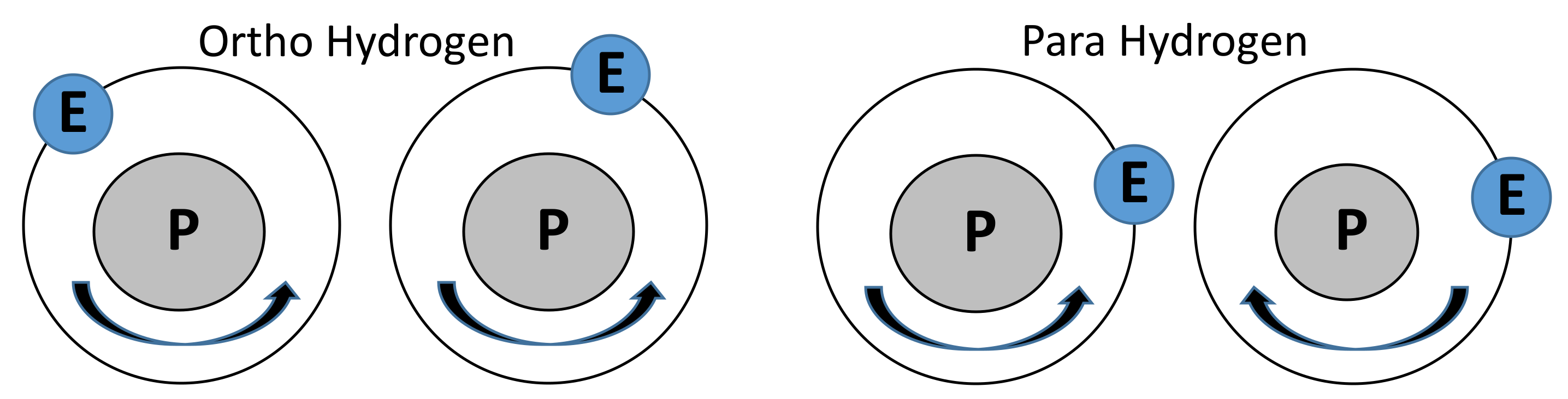
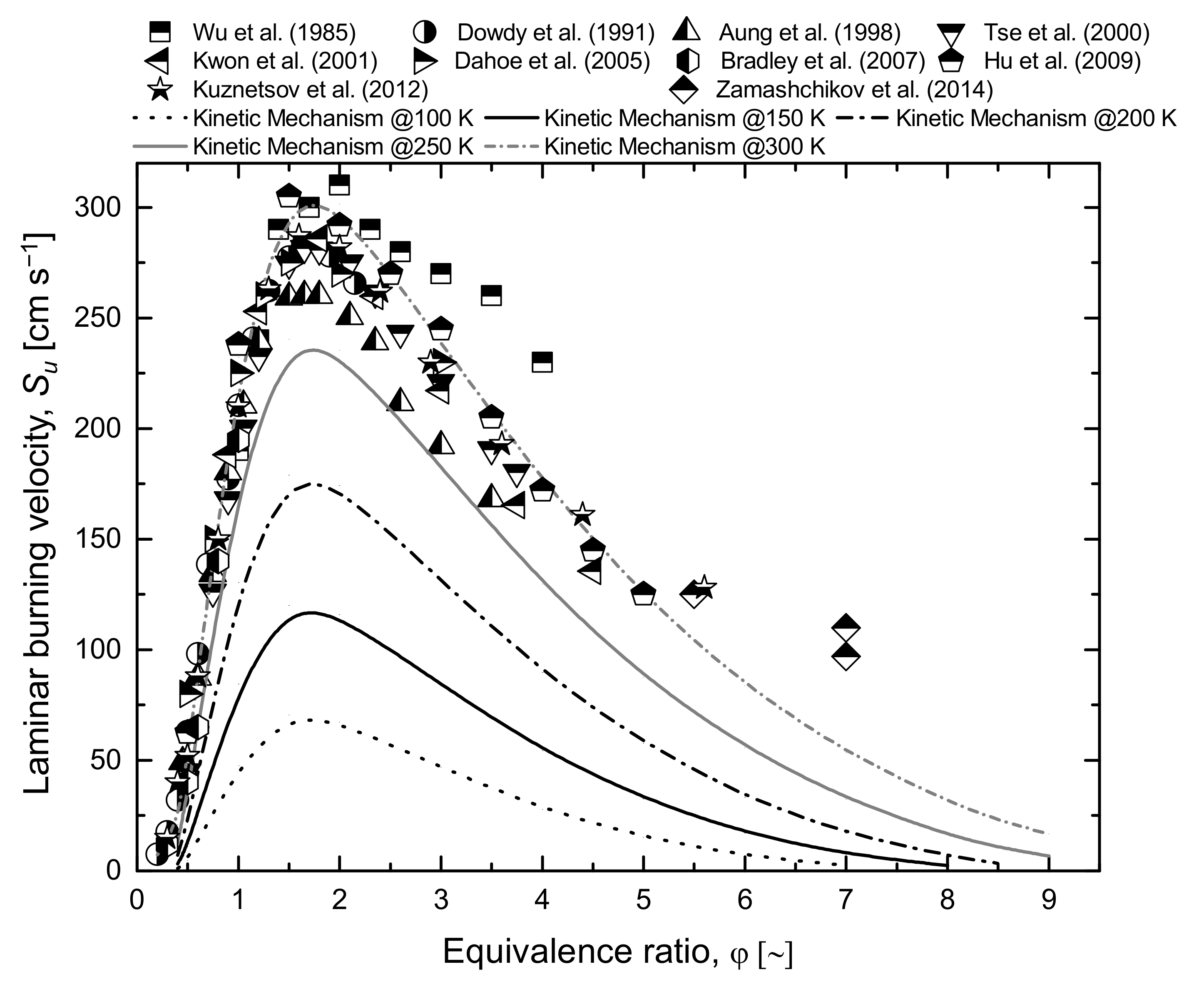
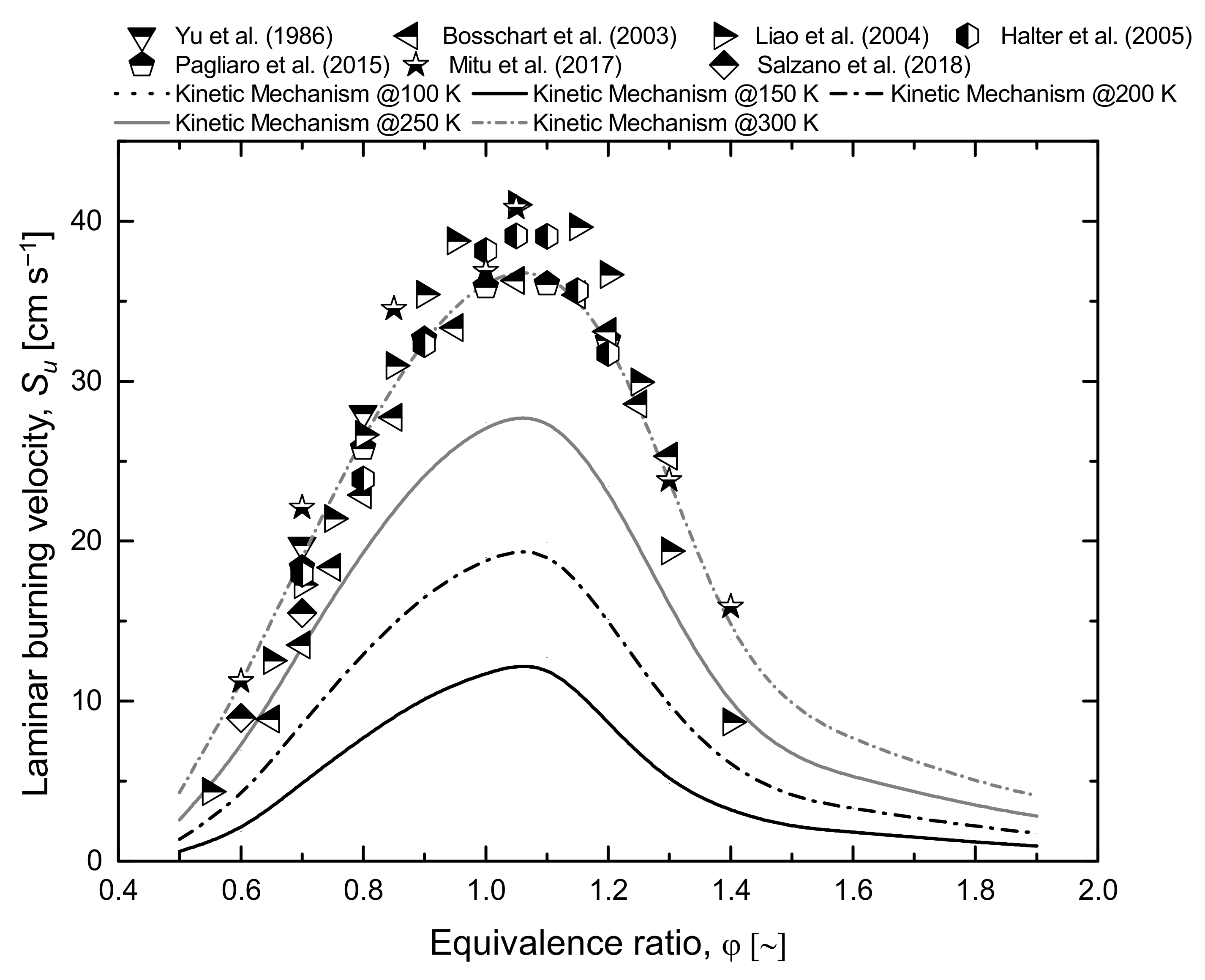
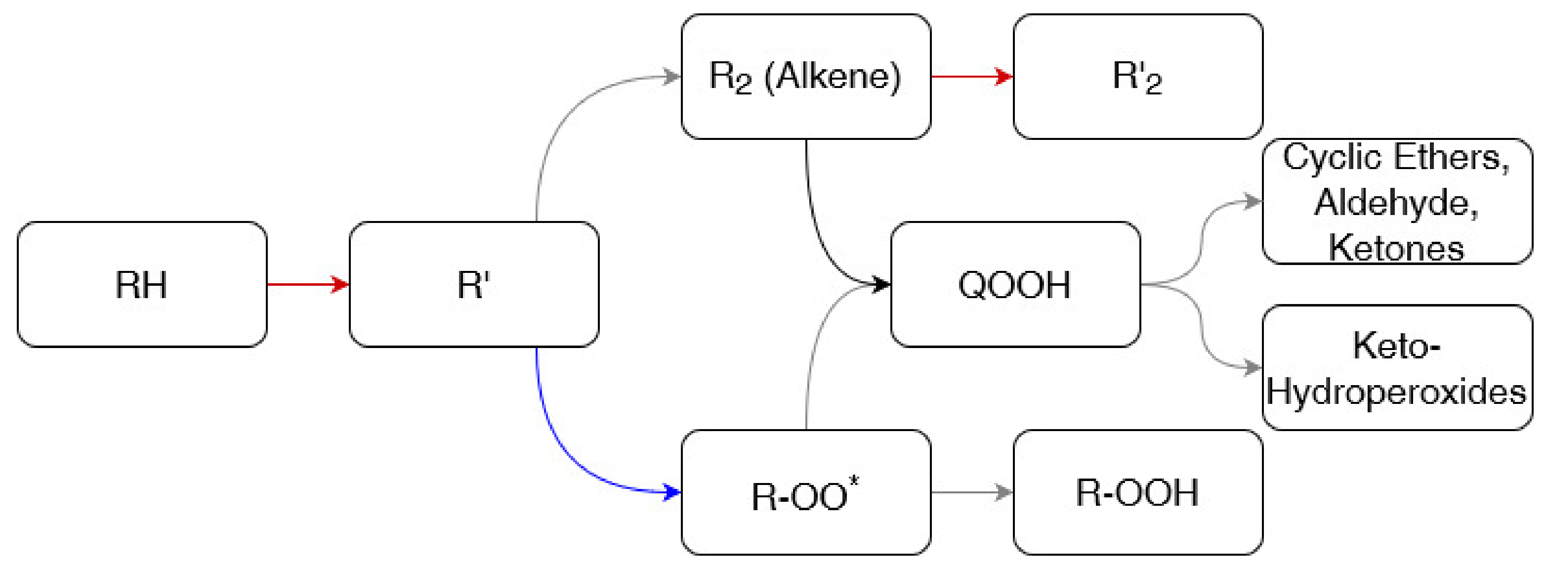
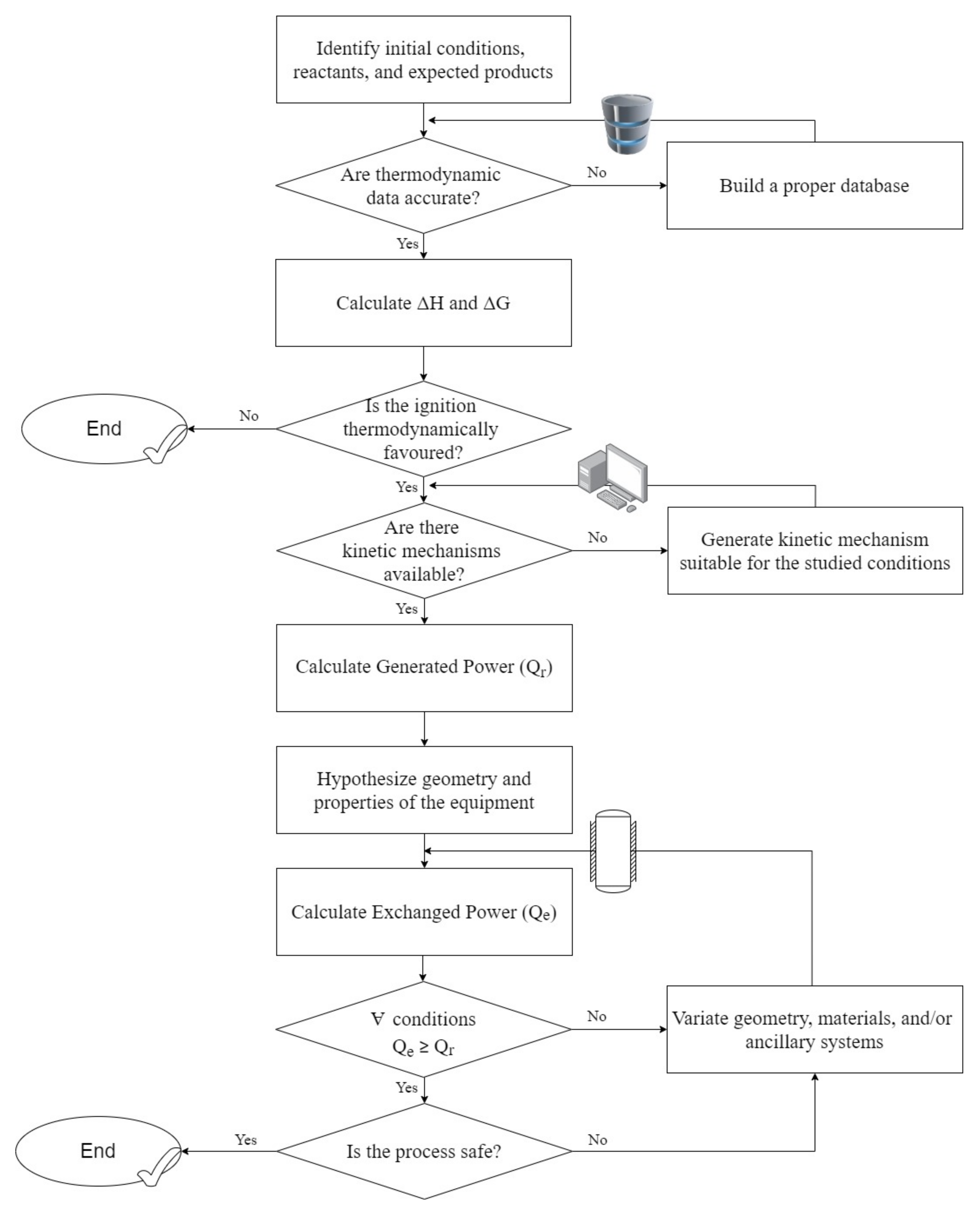
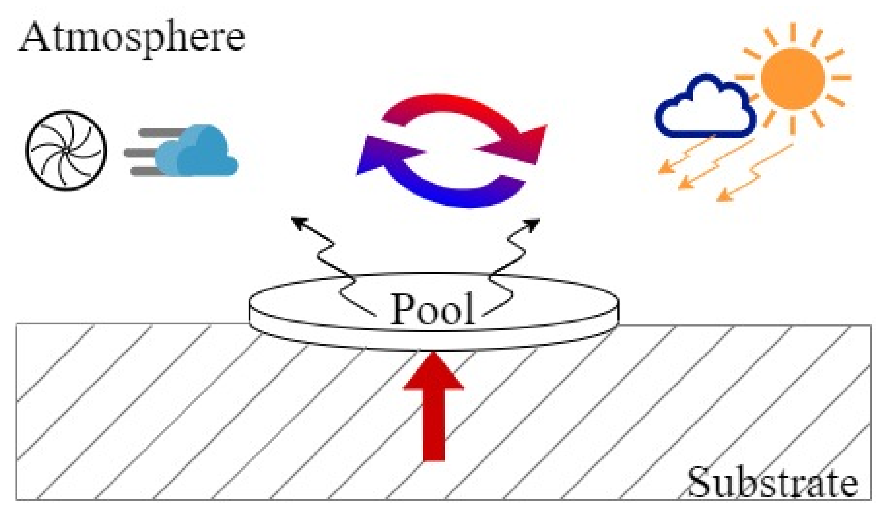
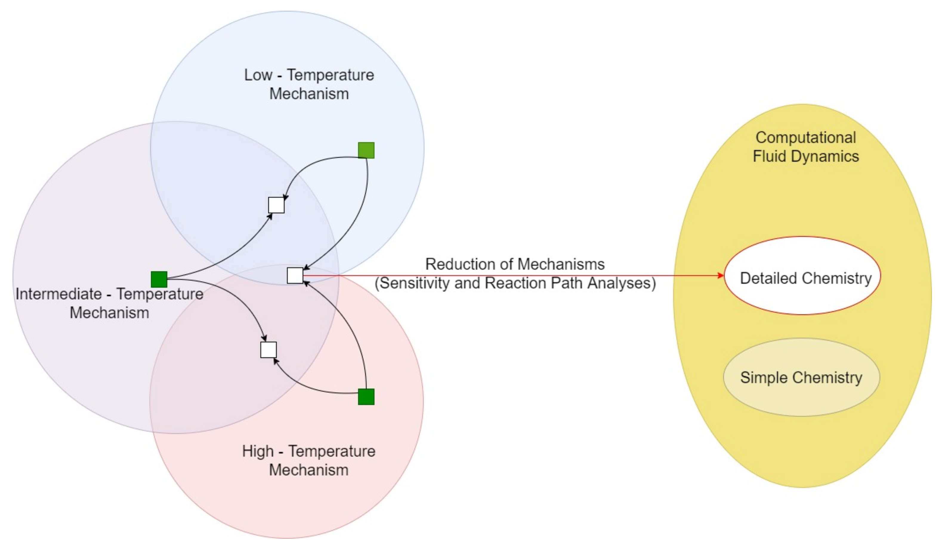
Table 1.
Low-temperature coefficients of NASA polynomial, as obtained by ab initio calculations for species involved in an accidental release of cryogenic fuels in the atmosphere [38,39].
| Species | A0 | A1 | A2 | A3 | A4 | A5 | A6 |
|---|---|---|---|---|---|---|---|
| n-H2 | 3.50 × 100 | 7.97 × 10⁻⁵ | −2.55 × 10⁻⁷ | 3.61 × 10⁻¹¹ | 2.69 × 10⁻¹³ | −1.06 × 10³ | −4.28 × 100 |
| o-H2 | 2.55 × 100 | −1.96 × 10⁻³ | 4.08 × 10⁻⁶ | 2.06 × 10⁻⁷ | −5.69 × 10⁻¹⁰ | −9.04 × 10² | 1.81 × 100 |
| p-H2 | 2.61 × 100 | −1.39 × 10⁻² | 3.39 × 10⁻⁴ | −1.61 × 10⁻⁶ | 2.22 × 10⁻⁹ | −1.06 × 10³ | −3.59 × 10⁻¹ |
| CH4 | 4.21 × 100 | −5.36 × 10⁻³ | 2.51 × 10⁻⁵ | −2.14 × 10⁻⁸ | 5.97 × 10⁻¹² | −1.02 × 10⁴ | −9.21 × 10⁻¹ |
| C2H6 | 3.75 × 100 | 4.55 × 10⁻⁵ | 4.08 × 10⁻⁵ | −4.57 × 10⁻⁸ | 1.57 × 10⁻¹¹ | −1.15 × 10⁴ | 4.74 × 100 |
| C3H8 | 3.06 × 100 | 1.29 × 10⁻² | 3.47 × 10⁻⁵ | −4.71 × 10⁻⁸ | 1.71 × 10⁻¹¹ | −1.44 × 10⁴ | 1.08 × 101 |
| N2 | 3.54 × 100 | −6.93 × 10⁻⁴ | 2.10 × 10⁻⁶ | −1.29 × 10⁻⁹ | 2.59 × 10⁻¹³ | −1.04 × 10³ | 2.99 × 100 |
| O2 | 3.12 × 100 | 1.73 × 10⁻³ | −8.53 × 10⁻⁷ | 1.70 × 10⁻¹⁰ | −1.23 × 10⁻¹⁴ | −1.04 × 10³ | 6.28 × 100 |
Table 2.
Main characteristics of the commonly used standard methods for FLs determination.
| Characteristic | Typical Alternatives |
|---|---|
| Explosion vessel | Closed glass sphere or cylinder, Steel tube, Glass flask, Quartz tube |
| Flame direction | Horizontal, Vertical |
| Ignition source | Spark, Flame, Exploding wire |
| Ignition duration | 0.2 s, 0.5 s |
| Ignition position | Sphere centre, Tube bottom |
| Ignition criteria | Visual flame, Thermal rise, Pressure rise, Pressure-time curve inflexion point |
| Limit definition | Last non-ignition point, Average of last ignition and non-ignition points |
Table 3.
Gaseous compositions, expressed in volumetric fractions, typically considered as per LNG representation.
Table 3.
Gaseous compositions, expressed in volumetric fractions, typically considered as per LNG representation.
| Mixture | CH4 [% vol/vol] | C2H6 [%vol/vol] | C3H8 [%vol/vol] |
|---|---|---|---|
| LNG 1 | 100 | 0 | 0 |
| LNG 2 | 90 | 10 | 0 |
| LNG 3 | 80 | 10 | 10 |
Table 4.
A representative list of evaporation rate models suitable for cryogenic conditions. Readers may consider the following definitions for the symbols adopted in this table if missing in the previous paragraphs: = relaxation parameters for liquefaction and evaporation. = pool radius. = kinematic viscosity. = fuel diffusivity in air.= wind velocity. = density of the vapor at saturation or air temperatures, or of the liquid at saturation temperature. = gravitational acceleration. = Boolean operator equal to 1 for and equal to 0 for .
| Authors [Reference] | Equation |
|---|---|
| Hertz-Knudsen-Schrage [115,116] | |
| Ingersoll [117] | |
| Mackay and Matsugu [118] | |
| Lee [119] | |
| Raj and Morris [120] | |
| Reed [121] | |
| Hummel [122] | |
| Barry [123] | |
| Derek et al. [124] | |
| Heymes [125] | |
| Schrage [126] |
Publisher’s Note: MDPI stays neutral with regard to jurisdictional claims in published maps and institutional affiliations. |
© 2021 by the authors. Licensee MDPI, Basel, Switzerland. This article is an open access article distributed under the terms and conditions of the Creative Commons Attribution (CC BY) license (https://creativecommons.org/licenses/by/4.0/).
Share and Cite
MDPI and ACS Style
Pio, G.; Salzano, E. Accidental Combustion Phenomena at Cryogenic Conditions. Safety 2021, 7, 67. https://0-doi-org.brum.beds.ac.uk/10.3390/safety7040067
AMA Style
Pio G, Salzano E. Accidental Combustion Phenomena at Cryogenic Conditions. Safety. 2021; 7(4):67. https://0-doi-org.brum.beds.ac.uk/10.3390/safety7040067
Chicago/Turabian StylePio, Gianmaria, and Ernesto Salzano. 2021. "Accidental Combustion Phenomena at Cryogenic Conditions" Safety 7, no. 4: 67. https://0-doi-org.brum.beds.ac.uk/10.3390/safety7040067
Note that from the first issue of 2016, this journal uses article numbers instead of page numbers. See further details here.