

Improved Differential Evolution Algorithm Guided by Best and Worst Positions Exploration Dynamics

1
ASH (Mathematics) Department, REC Bijnor, Chandpur 246725, UP, India
2
Department of Basic Sciences, Preparatory Year, King Faisal University, Al Ahsa 31982, Saudi Arabia
*
Author to whom correspondence should be addressed.
Biomimetics 2024, 9(2), 119; https://0-doi-org.brum.beds.ac.uk/10.3390/biomimetics9020119
Submission received: 27 November 2023
/
Revised: 26 January 2024
/
Accepted: 10 February 2024
/
Published: 16 February 2024
(This article belongs to the Special Issue Nature-Inspired Metaheuristic Optimization Algorithms 2024)
Abstract
:The exploration of premium and new locations is regarded as a fundamental function of every evolutionary algorithm. This is achieved using the crossover and mutation stages of the differential evolution (DE) method. A best-and-worst position-guided novel exploration approach for the DE algorithm is provided in this study. The proposed version, known as “Improved DE with Best and Worst positions (IDEBW)”, offers a more advantageous alternative for exploring new locations, either proceeding directly towards the best location or evacuating the worst location. The performance of the proposed IDEBW is investigated and compared with other DE variants and meta-heuristics algorithms based on 42 benchmark functions, including 13 classical and 29 non-traditional IEEE CEC-2017 test functions and 3 real-life applications of the IEEE CEC-2011 test suite. The results prove that the proposed approach successfully completes its task and makes the DE algorithm more efficient.
1. Introduction
Nowadays, the optimization problems of various science and engineering domains are becoming more complex due to the presence of various algorithmic properties like differentiability, non-convexity, non-linearity, etc., and hence it is not possible to deal with them using traditional methods. For that reason, new meta-heuristic methods are emerging to deal with these challenges in optimization fields. A meta-heuristic is a general term for heuristic methods that can be useful in a wider range of situations than the precise conditions of any specific problem. These meta-heuristic methods can be categorized into different groups, such as (i) the EA-based group, e.g., genetic algorithm [1], differential evolution algorithm [2], Jaya algorithm [3], etc.; (ii) swarm-based group, e.g., particle swarm optimization [4], artificial bee colony [5], gray wolf optimization [6], whale optimization algorithm [7], manta ray foraging optimization [8], reptile search algorithm [9], etc.; (iii) physics-based group, e.g., gravitational search algorithm [10], sine-cosine algorithm [11], atom search optimization [12], etc.; and (iv) human-based group, e.g., brain storm optimization [13], teaching–learning-based optimization [14], gaining–sharing knowledge optimization [15], etc.
The DE algorithm has maintained its influence for the last three decades due to its excellent performance. Many of its variants have placed among the top ranks in the IEEE CEC conference series [16,17]. Its straight forward execution, simple and small structure, and quick convergence can be considered the main reasons for its great efficiency. It has been successfully applied to a wide range of real-life applications, such as image processing [18,19], industriel noise recognition [20], bit coin price forecasting [21], optimal power flow [22], neural network optimization [23], engineering design problems [24], and so on. There are also several other fields like controlling theory [25,26] which are also open for the application of the DE algorithm.
In spite of its many promising characteristics, DE also faces some shortcomings, such as stagnation problems, a slow convergence rate, and a failure to perform in many other critical situations. In the past three decades, a number of studies have been executed to improve its performance and overcome its shortcomings. Many improvements have been developed in the areas of mutation operation and control parameter adjustment. For example, Brest et al. [27] suggested a self-adaptive method of selecting control parameters F and Cr. Later, Zhang et al. [28] proposed JADE by adapting Cauchy distributed control parameters and the DE/current to p-best/2 strategy. Gong et al. [29] made self-adaptive rules to implement various mutation strategies with JADE. The idea behind JADE was further improved in SHADE [30] by maintaining a successful history memory of the control parameters. Later, LSHADE [31] was proposed to improve the search capacity of SHADE by adapting a linear population size reduction approach. Later, several enhanced variants, such as iLSHADE [32], LSHADE-SPA [33], LSHADE-CLM [34], and iLSHADE-RSP [35], were also presented to improve the performance of the LSHADE variant. The iLSHADE variant was also improved by Brest et al. in their new variant named jSO [36]
Despite these famous variants, there are many other DE variants that have been presented throughout the years, for which some diverse tactics have been adapted to modify the operation of mutation; for example, Ali et al. applied a Cauchy distribution-based mutation operation and proposed MDE [37]. Later, Choi et al. [38] modified the MDE and presented ACM-DE by adapting the advanced Cauchy mutation operator. Kumar and Pant presented MRLDE [39] by dividing the population into three sub regions in order to perform mutation operations. Mallipeddi et al. presented EPSDE [40] using ensemble mutation strategies. Gong and Cai [41] introduced a ranking-based selection idea of using vectors for mutation operation in the current population. Xiang et al. [42] combined two mutation strategies, DE/current/1/bin and DE/p-best/bin/1, to enhance the performance of the DE algorithm. Some recent research on the development of mutation operations is included in [43,44,45,46,47,48,49].
Apart from these, several good research projects have also been executed in different domains, such as improving population initializing strategies [50,51,52,53], crossover operations [54], selection operations [55,56], local exploration strategies [57,58,59], and so on.
An interesting and detailed literature survey on modifications in the DE algorithm over the last decades is given in [60].
It can be noticed that most of the advanced DE variants compromise their simple structure by including some supplementary features. Therefore, in order to enhance the performance of the DE algorithm without overly complicating its simple structure, a new exploration method guided by the best and worst positions is proposed in this paper. The proposed method attempts to optimally explore the search space by moving forward toward the best position or backward toward the worst position. Additionally, a DE/αbest/1 [39,42] approach is also incorporated with the proposed exploration strategies in the selection operation to achieve a better balance between exploitation and exploration. The proposed variant is termed as ‘IDEBW’ and has been implemented in various test cases and real-life applications.
The remaining of the paper is designed as follows: a concise description of DE is given in Section 2. The proposed approach for IDEBW variant is explained in Section 3. The parameter settings and the empirical results from various test suites and real-life applications are discussed in Section 4. Finally, the conclusion of the complete study is presented in Section 5.
2. DE Algorithm
A basic representation of DE can be expressed as DE/a/b/c, where ‘a’ stands for a mutation approach, ‘b’ stands for vector differences, and ‘c’ stands for a crossover approach. The various phases in the operation of the DE algorithm are explained next.
The working structure of the DE algorithm is very easy to implement. It begins with a random generated population of d-dimensional N-vectors within a specified bound domain [Yl, Yu], as shown in Equation (1).
Subsequently, the mutation, crossover, and selection phases are started for the generation and selection of new vectors for the next-generation population.
Mutation: This phase is considered as a key operation in the DE algorithm and can be used to explore new positions in the search space. Some mutation schemes to generate a perturbed vector, say, , are given in Equation (2).
where are mutually different vectors randomly chosen from ; the parameter is used to manage the magnification of the vector’s difference.
Crossover: This phase is generally responsible for maintaining the population diversity and generates a trail vector by blending the target and perturbed vector , as explained in Equation (3).
where isknown as the crossover parameter, and randi (D) denotes the random index used to ensure that at least one component in the trail vector is chosen from the mutant vector.
Selection: This procedure selects the best vector from the target and trail vectors for the next-generation population based on their fitness value, as determined by Equation (4).
3. Proposed IDEBW Algorithm
To improve the performance of the DE algorithm without making any major changes to its structure, we designed our variant IDEBW by modifying the original DE algorithm in two ways. We did this by first exploring the search area, guided by best and worst positions, and second by improving the selection operation, where a DE/αbest/1 approach is also incorporated to generate new trail vectors whenever the old trail vectors are not selected into the next generation. The proposed approaches are explained in detail as below:
3.1. Proposed Exploration Strategies
Rao [3] presented the idea of searching for new positions by going towards the best position and away from the worst positions, as shown in Equation (5).
Motivated by this remarkable idea, we have utilized this approach to explore new positions through mutation and crossover phases, as given below.
To find the new position Xi corresponding to the ith vector Yi, first we chose a random vector, say Yr, from the population and used Equations (6) and (7) to create the component of the Xi:
Crossover Operation by Best Position:
Crossover Operation by Worst Position:
where rand, randB and randW are different uniform random numbers from 0 to 1, and CRB and CRW are prefix constants used to handle the crossover rate. Now we can randomly pick any proposed crossover strategy on the basis of pre-fix probability, called ‘Pr’.
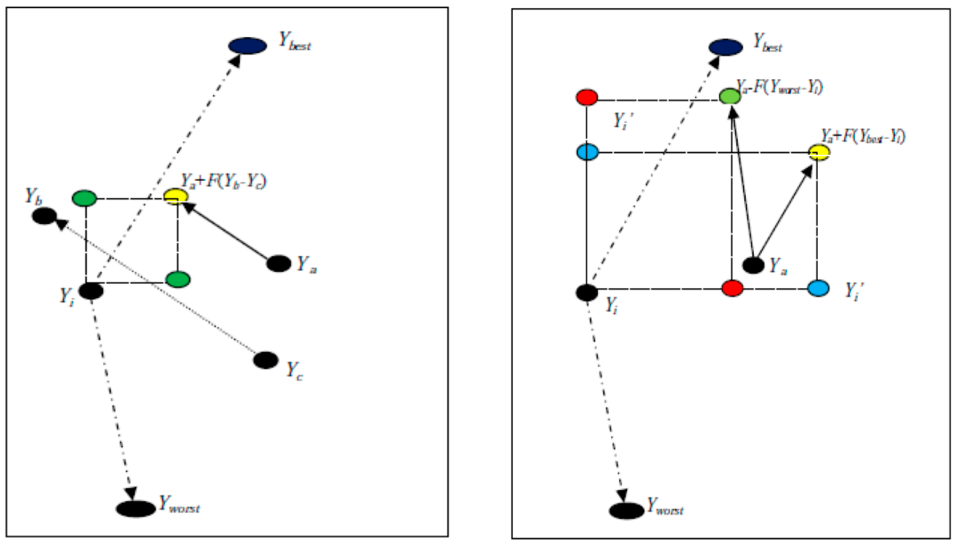
The difference between explorations by the DE/rand/1 and proposed strategies is graphically demonstrated in Figure 1. In the left image, the yellow and green dots represent the possible crossover position as determined using the DE/rand/1 strategy. When using this strategy, we can see that there are four possible crossover positions for the target vector Yi. In the right image, the yellow and blue dot represent the possible crossover position as assessed using the DE/rand/best/1 strategy, while the green and red dot represents the possible crossover position as determined using the DE/rand/worst/1 strategy. We can see that eight improved possible crossover positions for the target vector Yi are obtained using these strategies. Hence, we can say that the proposed strategies improve the exploration capability of the DE algorithm by providing additional and better positions for generating trail vectors compared to the DE/rand/1 approach.
3.2. Improved Selection Operation
If a vector created through the proposed crossover operation was not able to beat its target vector, then we imposed DE/αbest/1 to create an additional trail vector. This approach is an adapted version of DE/rand/1 and also utilizes the advantage of another approach, namely DE/best/1, by selecting the base vector Ya from the top α% of the current population. The crossover operation for the DE/αbest/1 is defined by Equation (8) as below:
where is a randomly selected vector from the top α% of the current population; and are another two randomly selected vectors; and and are control parameters.
Therefore, by using the proposed IDEBW, we not only obtain an additional approach to generating the trail vector, but also a way to improve it via a modified selection operation. However, apart from these advantages, we can also face drawbacks like slightly increased complexity and population stagnation problems in some cases.
The working steps, pseudo-code (Algorithm 1), and flowchart (Figure 2) of the proposed IDEBW are given as below:
- (a)
- Working Steps:
- Step-1:
- Initialize the parameter settings, like population size (N), CRB, CRW, CRα, Fα, probability constant (Pr), and Max-iteration, and generate initial population.
- Step-2:
- Generate a uniform random number rand and go to step-3.
- Step-3:
- If (rand ≤ Pr) then use Equation6; otherwise, use Equation (7) to generate trail vector.
- Step-4:
- Select this trail vector for the next generation if it gives a smaller fitness value than its corresponding target vector; otherwise, generate an additional trail vector using Equation (8) and repeat the old selection operation.
- Step-5:
- Repeat all above steps for all remaining vectors and obtain the best value after Max-iteration reached.
- (b)
- Pseudo-Code of proposed IDEBW
Algorithm 1. IDEBW Algorithm 1 Input: N, d, Max-iteration, CRB, CRW, CRα, Fα 2 via Equation (1) 3 Calculate function value f(Yi) for each i 4 While iteration ≤ Max_Iteration 5 Obtain best and worst locations 6 For i = 1:N 7 8 IF rand ≤ Pr 9 For j = 1:d 10 via Equation (6)//(DE/rand/best/1) 11 End For 12 Else 13 For j = 1:d 14 via Equation (7)//(DE/rand/best/1) 15 End For 16 End IF 17 IF 18 19 Update best position 20 Else 21 22 For j = 1:d 23 via Equation (8)//(DE/α-best/1) 24 End For 25 IF 26 27 Update best position 28 End IF 29 End IF 30 End For 31 iteration = iteration + 1 32 End While - (c)
- Flow Chart of proposed IDEBW
Figure 2.
Flow chart of IDEBW.

4. Result Analysis and Discussion
The performance assessment of the proposed IDEBW on various test suites and real-life problems is discussed in this section.
4.1. Experimental Settings
All experiments are executed under the following conditions:
- System Configuration: OS-64 Bit, Windows-10, Processor: 2.6-GHz Intel Core i3 processor, RAM-8GB.
- N=100; d=30,
- α = 20, Fα = 0.5, CRα = 0.9, CRB = 0.9, CRW = 0.5.
- Max-iteration = 100 × d.
- Total Run = 30.
4.2. Performance Evaluation of IDEBWon Classical Functions
A test suite of 13 simple and classical benchmark problems is selected from different studies [21,22,23]. The functions can be classified as unimodal (f1–f6) and multimodal functions (f8–f13),or as noisy function f7. As per the literature, the unimodal and multimodal functions are essential to testing the exploration and convergence effectiveness of the algorithms.
The performance assessment of IDEBW is performed with six other state-of-the-art DE variants, such as jDE [27], JADE [28], ApadapSS-JADE [29], SHADE [30], CJADE [58],and DEGOS [57]. The results for the jDE and JADE are copied from [28], while the results for the APadapSS-JADE are taken from [29]. For the SHADE, CJADE, and DEGOS, the results are obtained by using the code provided by the respective authors on http://toyamaailab.githhub.io/soucedata.html (accessed on 23 July 2023). The numerical results for the average error and standard deviation of 30 independent runs are presented in Table 1.
From Table 1, it is clear that the proposed IDEBW improves the quality of result, obtaining first rank for eight functions, namely f1, f2, f3, f5, f10, f11, f12, and f13, and second rank for function f6. For remaining functions f4 and f7, it takes third rank, while for f8 and f9, it takes sixth and fifth ranks, respectively. The Ap-AdapSS-JADE obtains first rank in three cases—f6, f7, and f11—whereas SHADE, JADE and jDE obtain first rank for f4, f9 and f8, respectively. The win/loss/tie (w/l/t) represents the pairwise competition which indicates that the IDEBW exceeds the CJADE, DEGOS, SHADE, AdapSS-JADE, JADE, and jDE in 10, 13, 10, 8, 11 and 11 cases, respectively.
To check the time complexity of the algorithm, the average CPU run time is also calculated for the algorithms IDEBW, CJADE, DEGOS, and SHADE. We can see that the CPU times for IDEBW, CJADE, DEGOS, and SHADE are 11.6, 13.2, 11.4 and 12.1 s, respectively. Hence, IDEBW takes less computing time than CJADE and SHADE. The exception is DEGOS, which is better than all algorithms in terms of time complexity.
The signs ‘+’, ‘−‘ and ‘=’ stand for whether the IDEBW is significantly better, worse, or equal, respectively. The p-value for pairwise ‘Wilcoxon sign test’ is also presented in the table, verifying the statistical effectiveness of the proposed IDEBW on the others.
The Wilcoxon rank sum test outcomes are listed in Table 2. The results present pairwise ranks, sum of ranks, and p-values. The lower rank and higher positive rank sum evidence the effectiveness of the proposed IDEBW over its competitors. However, the p-values shows that the IDEBW is significantly better than CJADE, DEGOS, and jDE, while there is no significant difference between the performance of IDEBW, SHADE, APAdapSS-JADE, and JADE.
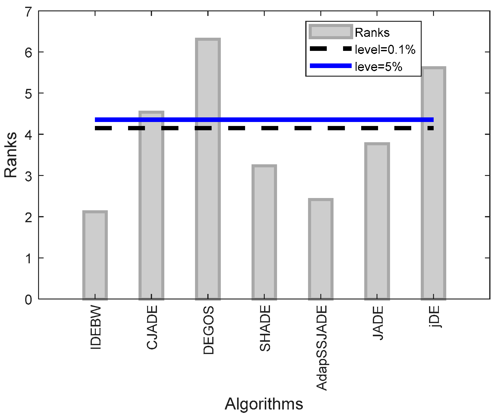
The Friedman’s rank and critical difference (CD) values obtained through the Bonferroni–Dunn test are presented in Table 3 in order to examine the global difference between the algorithms. The IDEBW obtained the lowest average rank, confirming its significance over others.
Figure 3 represents the algorithm’s ranks and horizontal control lines. These show significant levels at 10% and 5%, respectively. Through the graph, we can see that the rank bars of the IDEBW, SHADE, ApadapSS-JADE, and JADE are below the control lines and hence these algorithms are of equal significance, while the CJADE, DEGOS, and jDE are considered significantly worse than the obtained IDEBW algorithm.
Figure 4 represents the convergence graphs of the algorithms for some selected functions: f1, f2, f10 and f11. The X- and Y-axes indicate the iterations and fitness values of the function. We can analyze the convergence behaviour of the algorithms using their graph lines, which verifies the faster convergence of the proposed IDEBW than its competitors.
4.3. Performance Evaluation of IDEBW on CEC2017 Functions
In this section, a performance assessment of the IDEBW is performed on a well-known IEEE CEC-2017 test suite of 29 (C1–C30) more complicated and composite functions. These functions can be divided into four groups: unimodal (C1–C3), multimodal (C4–C10), hybrid (C11–C20), and composite (C21–C30). For a function, the optimum value is , while the initial bounds are (−100, 100) for all functions. A full specification of these functions is given in [61].
Next the performance Assessment of IDEBW with DE Variants and other meta-heuristics have been carried out separately and their numerical results are presented in Table 4 and Table 5 respectively while the statistical analysis on these results are given in Table 6 and Table 7.
4.3.1. Performance Assessment with DE Variants
Five state-of-the-art DE variants, such as SHADE [30], DEGOS [57], CJADE [58], TRADE [59] and IMODE [62] are selected for performance assessment with IDEBW. The TRADE, CJADE, and DEGOS are recently developed DE variants, while the SHADE and IMODE are the winner algorithms from the CEC-2014 and CEC-2020 competitions, respectively. The population size and maximum iterations are taken as 100 and 3000, respectively, for all algorithms. The other parameter settings of algorithms are taken as suggested in their original works.
Table 4 presents the numerical results for the average error and standard deviation of 30 runs. The value to reach (VTR) is taken as 10−08, i.e., the error is taken as 0 if it crosses the fixed VTR. Table 4 shows that the IDEBW obtains first rank in 11 cases, such as C1, C6, C9, C13, C15, C18, C19, C22, C25, C29 and C30. Similarly, TRADE obtains first rank in 11 cases, such as C1, C6, C9, C16, C17, C20, C22, C23, C25, C26 and C27. SHADE obtains best position in 10 cases, such as C1, C3, C5, C7, C8, C10, C21, C22, C24, and C25. The CJADE and DEGOS both obtain first ranks in 5 cases such as (C1, C6, C9, C22, and C25) and (C1, C9, C11, C14, and C22), respectively, whereas IMODE takes first place in only 3 cases, such as C4, C12, and C28. All algorithms except IMODE equally obtain first rank for C1 and C22, while the IDEBW, TRADE, DEGOS and CJADE perform equally in the case of C6 and C9. The pairwise w/l/t performance demonstrates that the IDEBW exceeds the TRADE, CJADE, DEGOS, SHADE, and IMODE in 13, 14, 16, 14 and 25 cases, respectively.
The average CPU times for the IDEBW, TRADE, CJADE, DEGOS, SHADE and IMODE are 146.2, 165.4, 172.9, 144.5, 148.1, and 168.2 s, respectively. Hence, IDEBW takes less computing time than all DE variants except DEGOS, which is better than all algorithms in term of time complexity.
The p-values obtained by the pairwise ‘Wilcoxon sign test’ also verify the statistical effectiveness of the proposed IDEBW on the others.
The Wilcoxon rank sum test outcomes with pairwise ranks, sum of ranks, and p-values are listed in Table 6. The lower rank and higher positive rank sum evidence the effectiveness of the proposed IDEBW over its competitors. However, the p-values show that the IDEBW is significantly better than IMODE, while there is no significant difference between the performance of the IDEBW, TRADE, CJADE, DEGOS, and SHADE.
The Friedman’s rank and critical difference (CD) values obtained through the Bonferroni–Dunn test are presented in Table 7 to test out the global difference between the algorithms. The TRADE obtained lowest average rank; however, the bar graphs presented in Figure 5a shows that the IDEBW, TRADE, DEGOS, and SHADE are considered as significantly equal, while the CJADE and IMODE are significantly worse with these algorithms.
4.3.2. Performance Assessment with Other Meta-Heuristics
In this section, the performance of the IDEBW is compared with that of 5 other meta-heuristics algorithms such as TDSD [63], EJaya [64], AGBSO [65], HMRFO [66],and disGSA [67]. The HMRFO, disGSA, AGBSO, and EJaya methods are recently developed variants of meta-heuristics such as MRFO, GSA, BSO, and Jaya algorithms, respectively, whereas the TDSD is a hybrid variant of three search dynamics such as spherical search, hypercube search, and chaotic local search.
The population size and maximum iterations are taken as 100 and 3000, respectively, for all algorithms. The other parameter settings of algorithms are taken as suggested in their original works.
Table 5 presents the obtained average error and standard deviation of 30 runs. The Table 5 shows that IDEBW obtains first rank in 14 cases, namely, C1, C6, C9, C11, C13, C14, C15, C18, C19, C20, C22, C27, C29,and C30, whereas AGBSO obtains first rank in 9 cases C5, C8, C9, C10, C16, C17, C21, C22, and C23. The EJAYA, HMRFO, disGSA, and TDSD obtain first ranks in 3 cases (C3, C12, and C22), 1 case (C22), 4 cases (C7, C22, C24, and C26), and 2 cases (C4, C25), respectively. The pairwise w/l/t demonstrates that the IDEBW exceeds the EJAYA, HMRFO, AGBSO, disGSA, and TDSD on 24, 25, 16, 17 and 22 cases, respectively.
The average CPU times for IDEBW, EJAYA, HMRFO, AGBSO, DisGSA, and TDSD are 146.2, 105.4, 165.2, 154.4, 159.2, and 189.3 s, respectively. Hence, IDEBW takes less computing time than all meta-heuristics except EJAYA, which is better than all algorithms in term of time complexity.
The p-values, obtained by the pairwise ‘Wilcoxon sign test’, also verify the statistical effectiveness of the proposed IDEBW on the others.
The Wilcoxon rank sum test outcomes with pairwise ranks, sum of ranks, and p-values are listed in Table 6. The lower rank and higher positive rank sum evidence the effectiveness of the proposed IDEBW over its competitors. The p-values show that only AGBSO demonstrated a significantly equal performance with the IDEBW, whereas all other meta-heuristics are significantly worst against the IDEBW.
The Friedman’s rank and critical difference (CD) values obtained through the Bonferroni–Dunn test are presented in Table 7 to test out the global difference between the algorithms. The IDEBW obtains the lowest average rank and shows its significance.
The bar graphs presented in Figure 5b show that the IDEBW and AGBSO are significantly equal, while the others cross the control lines and are considered as significantly worse compared to those with these algorithms.
Figure 6 represents the convergence graphs of the algorithms for some selected functions: C1, C10, C21, and C30. The X and Y-axes indicate the iterations and fitness values of the function. We can analyze the convergence behaviour of the algorithms by their graphs lines, which verify the faster convergence of the proposed IDEBW on its competitors.
4.4. Performance Evaluation of IDEBW on Real-Life Applications
In this section, the practical qualification of the proposed IDEBW is tested on 03 IEEE CEC-2011 real-life applications, as given below:
- RP1:
- Frequency-modulated (FM) sound wave problem.
- RP2:
- Spread-spectrum radar polyphase code design problem.
- RP3:
- Non-linear stirred tank reactor optimal control problem.
The complete details of these problems are specified in [68].
The performance assessment is taken with five qualified algorithms, including DEGOS, SHADE, DE, EJAYA, and TDSD. The outcomes for the SHADE and TDSD are copied from [63]. The maximum iterations are taken as 100 × d, i.e., it is 600, 2000, and 100 for the RP1, RP2, and RP3 respectively. The results for the best values, mean values and standard deviation obtained in 30 independent runs are presented in Table 8.
The results show that the proposed IDEBW improves the quality of results and obtains first rank by obtaining the optimum value in each case, whether it is RP1, RP2,and RP3. The SHADE algorithm takes second rank for RP1 and RP2, while TDSD takes second rank for RP3. Hence, the proposed IDEBW confirms its feasibility for use on the real-life problems also.
The convergence graphs for the IDEBW, DEGOS, DE, and EJAYA are presented in Figure 7. The X- and Y-axes indicate the iterations and fitness values of the function. We can analyze the convergence behaviour of the algorithms by their graph lines, which also demonstrate a faster convergence speed of the IDEBW compared to its opponents.
5. Conclusions
A best and worst location guided exploration approach to the DE algorithm is presented in this study. The proposed technique offers an improved search alternative by either directing attention towards the best location or avoiding the most unfavorable location. The proposed variant named ‘IDEBW’ also uses the DE/αbest/1 approach as a selection operation when the trail vectors are not selected for the next operation. The ‘IDEBW’ variant is tested on 13 classical, 29 hybrids, and composite CEC-17 benchmark functions and 3 real-life optimization problems from the CEC-2011 test suite. The results are compared with eight other state-of-the-art DE variants, such as jDE, JADE, SHADE, APadapSS-JADE, CJADE, DEGOS, TRADE, and IMODE, and 5 other enhanced meta-heuristics variants, such as EJAYA, HMRFO, disGSA, AGBSO, and TDSD. The outcomes verify the success of the new exploration strategy in terms of improvement in solution quality, as well as in convergence speed.
Our future works will focus on employing the proposed IDEBW in some complicated, constrained, and multi-objective real-life applications. Second, it will also be quite exciting to apply the proposed idea to other meta-heuristic algorithms to improve their performance.
Author Contributions
Conceptualization, P.K.; methodology, P.K.; software, P.K. and M.A.; validation, P.K. and M.A.; formal analysis, P.K.; investigation, P.K. and M.A.; resources, P.K. and M.A.; data curation, P.K.; writing—original draft preparation, P.K. and M.A.; writing—review and editing, P.K. and M.A.; visualization, P.K. and M.A.; supervision, P.K. and M.A.; project administration, P.K.; funding acquisition, M.A. All authors have read and agreed to the published version of the manuscript.
Funding
This work was supported by the Deanship of Scientific Research, Vice Presidency for Graduate Studies and Scientific Research, King Faisal University, Saudi Arabia (Grant No. 5806).
Institutional Review Board Statement
Not applicable.
Data Availability Statement
All related data is contained within the article.
Conflicts of Interest
The authors declare no conflicts of interest.
References
- Wright, A.H. Genetic Algorithms for Real Parameter Optimization. Found. Genet. Algorithms 1991, 1, 205–218. [Google Scholar] [CrossRef]
- Storn, R.; Price, K. Differential Evolution—A Simple and Efficient Heuristic for Global Optimization over Continuous Spaces. J. Glob. Optim. 1997, 11, 341–359. [Google Scholar] [CrossRef]
- Venkata Rao, R. Jaya: A Simple and New Optimization Algorithm for Solving Constrained and Unconstrained Optimization Problems. Int. J. Ind. Eng. Comput. 2016, 7, 19–34. [Google Scholar] [CrossRef]
- Kennedy, J.; Eberhart, R. Particle Swarm Optimization. In Proceedings of the IEEE International Conference on Neural Networks, Perth, WA, Australia, 27 November–1 December 1995; Volume IV, pp. 1942–1948. [Google Scholar]
- Karaboga, D.; Basturk, B. A Powerful and Efficient Algorithm for Numerical Function Optimization: Artificial Bee Colony (ABC) Algorithm. J. Glob. Optim. 2007, 39, 459–471. [Google Scholar] [CrossRef]
- Mirjalili, S.; Mirjalili, S.M.; Lewis, A. Grey Wolf Optimizer. Adv. Eng. Softw. 2014, 69, 46–61. [Google Scholar] [CrossRef]
- Mirjalili, S.; Lewis, A. The Whale Optimization Algorithm. Adv. Eng. Softw. 2016, 95, 51–67. [Google Scholar] [CrossRef]
- Zhao, W.; Zhang, Z.; Wang, L. Manta Ray Foraging Optimization: An Effective Bio-Inspired Optimizer for Engineering Applications. Eng. Appl. Artif. Intell. 2020, 87, 103300. [Google Scholar] [CrossRef]
- Abualigah, L.; Elaziz, M.A.; Sumari, P.; Geem, Z.W.; Gandomi, A.H. Reptile Search Algorithm (RSA): A Nature-Inspired Meta-Heuristic Optimizer. Expert Syst. Appl. 2022, 191, 116158. [Google Scholar] [CrossRef]
- Rashedi, E.; Nezamabadi-pour, H.; Saryazdi, S. GSA: A Gravitational Search Algorithm. Inf. Sci. 2009, 179, 223–2248. [Google Scholar] [CrossRef]
- Mirjalili, S. SCA: A Sine Cosine Algorithm for Solving Optimization Problems. Knowl.-Based Syst. 2016, 96, 120–133. [Google Scholar] [CrossRef]
- Zhao, W.; Wang, L.; Zhang, Z. A Novel Atom Search Optimization for Dispersion Coefficient Estimation in Groundwater. Futur. Gener. Comput. Syst. 2019, 91, 601–610. [Google Scholar] [CrossRef]
- Shi, Y. Brain Storm Optimization Algorithm. In Lecture Notes in Computer Science; Springer: Berlin/Heidelberg, Germany, 2011. [Google Scholar]
- Rao, R.V.; Savsani, V.J.; Vakharia, D.P. Teaching-Learning-Based Optimization: A Novel Method for Constrained Mechanical Design Optimization Problems. CAD Comput. Aided Des. 2011, 43, 303–315. [Google Scholar] [CrossRef]
- Mohamed, A.W.; Hadi, A.A.; Mohamed, A.K. Gaining-Sharing Knowledge Based Algorithm for Solving Optimization Problems: A Novel Nature-Inspired Algorithm. Int. J. Mach. Learn. Cybern. 2020, 11, 1501–1529. [Google Scholar] [CrossRef]
- Deng, L.B.; Zhang, L.L.; Fu, N.; Sun, H.L.; Qiao, L.Y. ERG-DE: An Elites Regeneration Framework for Differential Evolution. Inf. Sci. 2020, 539, 81–103. [Google Scholar] [CrossRef]
- Zhang, K.; Yu, Y. An Enhancing Differential Evolution Algorithm with a Rankup Selection: RUSDE. Mathematics 2021, 9, 569. [Google Scholar] [CrossRef]
- Kumar, S.; Kumar, P.; Sharma, T.K.; Pant, M. Bi-Level Thresholding Using PSO, Artificial Bee Colony and MRLDE Embedded with Otsu Method. Memetic Comput. 2013, 5, 323–334. [Google Scholar] [CrossRef]
- Chakraborty, S.; Saha, A.K.; Ezugwu, A.E.; Agushaka, J.O.; Zitar, R.A.; Abualigah, L. Differential Evolution and Its Applications in Image Processing Problems: A Comprehensive Review. Arch. Comput. Methods Eng. 2023, 30, 985–1040. [Google Scholar] [CrossRef]
- Kumar, P.; Pant, M. Recognition of Noise Source in Multi Sounds Field by Modified Random Localized Based DE Algorithm. Int. J. Syst. Assur. Eng. Manag. 2018, 9, 245–261. [Google Scholar] [CrossRef]
- Jana, R.K.; Ghosh, I.; Das, D. A Differential Evolution-Based Regression Framework for Forecasting Bitcoin Price. Ann. Oper. Res. 2021, 306, 295–320. [Google Scholar] [CrossRef]
- Yi, W.; Lin, Z.; Lin, Y.; Xiong, S.; Yu, Z.; Chen, Y. Solving Optimal Power Flow Problem via Improved Constrained Adaptive Differential Evolution. Mathematics 2023, 11, 1250. [Google Scholar] [CrossRef]
- Baioletti, M.; Di Bari, G.; Milani, A.; Poggioni, V. Differential Evolution for Neural Networks Optimization. Mathematics 2020, 8, 69. [Google Scholar] [CrossRef]
- Mohamed, A.W. A Novel Differential Evolution Algorithm for Solving Constrained Engineering Optimization Problems. J. Intell. Manuf. 2018, 28, 149–164. [Google Scholar] [CrossRef]
- Chi, R.; Li, H.; Shen, D.; Hou, Z.; Huang, B. Enhanced P-Type Control: Indirect Adaptive Learning from Set-Point Updates. IEEE Trans. Automat. Contr. 2023, 68, 1600–1613. [Google Scholar] [CrossRef]
- Roman, R.-C.; Precup, R.-E.; Petriu, E.M.; Borlea, A.-I. Hybrid Data-Driven Active Disturbance Rejection Sliding Mode Control with Tower Crane Systems Validation. Sci. Technol. 2024, 27, 3–17. [Google Scholar]
- Brest, J.; Greiner, S.; Bošković, B.; Mernik, M.; Zumer, V. Self-Adapting Control Parameters in Differential Evolution: A Comparative Study on Numerical Benchmark Problems. IEEE Trans. Evol. Comput. 2006, 10, 646–657. [Google Scholar] [CrossRef]
- Zhang, J.; Sanderson, A.C. JADE: Adaptive Differential Evolution with Optional External Archive. IEEE Trans. Evol. Comput. 2009, 13, 945–958. [Google Scholar] [CrossRef]
- Gong, W.; Fialho, Á.; Cai, Z.; Li, H. Adaptive Strategy Selection in Differential Evolution for Numerical Optimization: An Empirical Study. Inf. Sci. 2011, 181, 5364–5386. [Google Scholar] [CrossRef]
- Tanabe, R.; Fukunaga, A. Success-History Based Parameter Adaptation for Differential Evolution. In Proceedings of the 2013 IEEE Congress on Evolutionary Computation, CEC 2013, Cancun, Mexico, 20–23 June 2013. [Google Scholar]
- Tanabe, R.; Fukunaga, A.S. Improving the Search Performance of SHADE Using Linear Population Size Reduction. In Proceedings of the 2014 IEEE Congress on Evolutionary Computation, CEC 2014, Beijing, China, 6–11 July 2014. [Google Scholar]
- Brest, J.; Maučec, M.S.; Bošković, B. IL-SHADE: Improved L-SHADE Algorithm for Single Objective Real-Parameter Optimization. In Proceedings of the 2016 IEEE Congress on Evolutionary Computation, CEC 2016, Vancouver, BC, Canada, 24–29 July 2016. [Google Scholar]
- Hadi, A.A.; Mohamed, A.W.; Jambi, K.M. LSHADE-SPA Memetic Framework for Solving Large-Scale Optimization Problems. Complex Intell. Syst. 2019, 5, 25–40. [Google Scholar] [CrossRef]
- Zhao, F.; Zhao, L.; Wang, L.; Song, H. A Collaborative LSHADE Algorithm with Comprehensive Learning Mechanism. Appl. Soft Comput. J. 2020, 96, 106609. [Google Scholar] [CrossRef]
- Choi, T.J.; Ahn, C.W. An Improved LSHADE-RSP Algorithm with the Cauchy Perturbation: ILSHADE-RSP. Knowl.-Based Syst. 2021, 215, 106628. [Google Scholar] [CrossRef]
- Brest, J.; Maučec, M.S.; Bošković, B. Single Objective Real-Parameter Optimization: Algorithm JSO. In Proceedings of the 2017 IEEE Congress on Evolutionary Computation, CEC 2017—Proceedings, Donostia, Spain, 5–8 June 2017. [Google Scholar]
- Ali, M.; Pant, M. Improving the Performance of Differential Evolution Algorithm Using Cauchy Mutation. Soft Comput. 2011, 15, 991–1007. [Google Scholar] [CrossRef]
- Choi, T.J.; Togelius, J.; Cheong, Y.G. Advanced Cauchy Mutation for Differential Evolution in Numerical Optimization. IEEE Access 2020, 8, 8720–8734. [Google Scholar] [CrossRef]
- Kumar, P.; Pant, M. Enhanced Mutation Strategy for Differential Evolution. In Proceedings of the 2012 IEEE Congress on Evolutionary Computation, CEC 2012, Brisbane, QLD, Australia, 10–15 June 2012. [Google Scholar]
- Mallipeddi, R.; Suganthan, P.N.; Pan, Q.K.; Tasgetiren, M.F. Differential Evolution Algorithm with Ensemble of Parameters and Mutation Strategies. Appl. Soft Comput. J. 2011, 11, 1679–1696. [Google Scholar] [CrossRef]
- Gong, W.; Cai, Z. Differential Evolution with Ranking-Based Mutation Operators. IEEE Trans. Cybern. 2013, 43, 2066–2081. [Google Scholar] [CrossRef]
- Xiang, W.L.; Meng, X.L.; An, M.Q.; Li, Y.Z.; Gao, M.X. An Enhanced Differential Evolution Algorithm Based on Multiple Mutation Strategies. Comput. Intell. Neurosci. 2015, 2015, 285730. [Google Scholar] [CrossRef]
- Gupta, S.; Su, R. An Efficient Differential Evolution with Fitness-Based Dynamic Mutation Strategy and Control Parameters. Knowl.-Based Syst. 2022, 251, 109280. [Google Scholar] [CrossRef]
- Wang, L.; Zhou, X.; Xie, T.; Liu, J.; Zhang, G. Adaptive Differential Evolution with Information Entropy-Based Mutation Strategy. IEEE Access 2021, 9, 146783–146796. [Google Scholar] [CrossRef]
- Sun, G.; Lan, Y.; Zhao, R. Differential Evolution with Gaussian Mutation and Dynamic Parameter Adjustment. Soft Comput. 2019, 23, 1615–1642. [Google Scholar] [CrossRef]
- Cheng, J.; Pan, Z.; Liang, H.; Gao, Z.; Gao, J. Differential Evolution Algorithm with Fitness and Diversity Ranking-Based Mutation Operator. Swarm Evol. Comput. 2021, 61, 100816. [Google Scholar] [CrossRef]
- Li, Y.; Wang, S.; Yang, B. An Improved Differential Evolution Algorithm with Dual Mutation Strategies Collaboration. Expert Syst. Appl. 2020, 153, 113451. [Google Scholar] [CrossRef]
- AlKhulaifi, D.; AlQahtani, M.; AlSadeq, Z.; ur Rahman, A.; Musleh, D. An Overview of Self-Adaptive Differential Evolution Algorithms with Mutation Strategy. Math. Model. Eng. Probl. 2022, 9, 1017–1024. [Google Scholar] [CrossRef]
- Kumar, P.; Ali, M. SaMDE: A Self Adaptive Choice of DNDE and SPIDE Algorithms with MRLDE. Biomimetics 2023, 8, 494. [Google Scholar] [CrossRef]
- Zhu, W.; Tang, Y.; Fang, J.A.; Zhang, W. Adaptive Population Tuning Scheme for Differential Evolution. Inf. Sci. 2013, 223, 164–191. [Google Scholar] [CrossRef]
- Poikolainen, I.; Neri, F.; Caraffini, F. Cluster-Based Population Initialization for Differential Evolution Frameworks. Inf. Sci. 2015, 297, 216–235. [Google Scholar] [CrossRef]
- Meng, Z.; Zhong, Y.; Yang, C. CS-DE: Cooperative Strategy Based Differential Evolution with Population Diversity Enhancement. Inf. Sci. 2021, 577, 663–696. [Google Scholar] [CrossRef]
- Stanovov, V.; Akhmedova, S.; Semenkin, E. Dual-Population Adaptive Differential Evolution Algorithm L-NTADE. Mathematics 2022, 10, 4666. [Google Scholar] [CrossRef]
- Meng, Z.; Chen, Y. Differential Evolution with Exponential Crossover Can Be Also Competitive on Numerical Optimization. Appl. Soft Comput. 2023, 146, 110750. [Google Scholar] [CrossRef]
- Zeng, Z.; Zhang, M.; Chen, T.; Hong, Z. A New Selection Operator for Differential Evolution Algorithm. Knowl. -Based Syst. 2021, 226, 107150. [Google Scholar] [CrossRef]
- Kumar, A.; Biswas, P.P.; Suganthan, P.N. Differential Evolution with Orthogonal Array-based Initialization and a Novel Selection Strategy. Swarm Evol. Comput. 2022, 68, 101010. [Google Scholar] [CrossRef]
- Yu, Y.; Gao, S.; Wang, Y.; Todo, Y. Global Optimum-Based Search Differential Evolution. IEEE/CAA J. Autom. Sin. 2019, 6, 379–394. [Google Scholar] [CrossRef]
- Gao, S.; Yu, Y.; Wang, Y.; Wang, J.; Cheng, J.; Zhou, M. Chaotic Local Search-Based Differential Evolution Algorithms for Optimization. IEEE Trans. Syst. Man, Cybern. Syst. 2021, 51, 3954–3967. [Google Scholar] [CrossRef]
- Cai, Z.; Yang, X.; Zhou, M.C.; Zhan, Z.H.; Gao, S. Toward Explicit Control between Exploration and Exploitation in Evolutionary Algorithms: A Case Study of Differential Evolution. Inf. Sci. 2023, 649, 119656. [Google Scholar] [CrossRef]
- Ahmad, M.F.; Isa, N.A.M.; Lim, W.H.; Ang, K.M. Differential Evolution: A Recent Review Based on State-of-the-Art Works. Alex. Eng. J. 2022, 61, 3831–3872. [Google Scholar] [CrossRef]
- Awad, N.H.; Ali, M.Z.; Liang, J.J.; Qu, B.Y.; Suganthan, P.N. Problem Definitions and Evaluation Criteria for the CEC 2017 Special Session and Competition on Single Objective Bound Constrained Real-Parameter Numerical Optimization; Technical Report; Nanyang Technological University: Singapore, 2016; pp. 1–34. [Google Scholar]
- Sallam, K.M.; Elsayed, S.M.; Chakrabortty, R.K.; Ryan, M.J. Improved Multi-Operator Differential Evolution Algorithm for Solving Unconstrained Problems. In Proceedings of the 2020 IEEE Congress on Evolutionary Computation, CEC 2020—Conference Proceedings, Glasgow, UK, 19–24 July 2020. [Google Scholar]
- Li, X.; Cai, Z.; Wang, Y.; Todo, Y.; Cheng, J.; Gao, S. TDSD: A New Evolutionary Algorithm Based on Triple Distinct Search Dynamics. IEEE Access 2020, 8, 76752–76764. [Google Scholar] [CrossRef]
- Zhang, Y.; Chi, A.; Mirjalili, S. Enhanced Jaya Algorithm: A Simple but Efficient Optimization Method for Constrained Engineering Design Problems. Knowl.-Based Syst. 2021, 233, 107555. [Google Scholar] [CrossRef]
- Cai, Z.; Gao, S.; Yang, X.; Yang, G.; Cheng, S.; Shi, Y. Alternate Search Pattern-Based Brain Storm Optimization. Knowl.-Based Syst. 2022, 238, 107896. [Google Scholar] [CrossRef]
- Tang, Z.; Wang, K.; Tao, S.; Todo, Y.; Wang, R.L.; Gao, S. Hierarchical Manta Ray Foraging Optimization with Weighted Fitness-Distance Balance Selection. Int. J. Comput. Intell. Syst. 2023, 16, 114. [Google Scholar] [CrossRef]
- Guo, A.; Wang, Y.; Guo, L.; Zhang, R.; Yu, Y.; Gao, S. An Adaptive Position-Guided Gravitational Search Algorithm for Function Optimization and Image Threshold Segmentation. Eng. Appl. Artif. Intell. 2023, 121, 106040. [Google Scholar] [CrossRef]
- Das, S.; Suganthan, P.N. Problem Definitions and Evaluation Criteria for CEC 2011 Competition on Testing Evolutionary Algorithms on Real World Optimization Problems; Jadavpur University: Kolkata, India; Nanyang Technological University: Singapore, 2010; pp. 341–359. [Google Scholar]
Figure 1.
Difference of exploration by DE/rand/mutation and proposed mutation.

Figure 3.
The Friedman ranks and Bonferroni–Dunn test presentation for classical functions.

Figure 4.
Performance evaluation of IDEBW by convergence graphs of classical functions. (a) F01 (Unimodal). (b) F02 (Unimodal). (c) F10 (Multimodal). (d) F11 (Multimodal).
Figure 4.
Performance evaluation of IDEBW by convergence graphs of classical functions. (a) F01 (Unimodal). (b) F02 (Unimodal). (c) F10 (Multimodal). (d) F11 (Multimodal).

Figure 5.
The Friedman ranks and Bonferroni–Dunn test presentation for CEC17 functions for (a) DE varaints. (b) Meta-hueristics varaints
Figure 5.
The Friedman ranks and Bonferroni–Dunn test presentation for CEC17 functions for (a) DE varaints. (b) Meta-hueristics varaints

Figure 6.
Convergence graphs for CEC-2017 functions: (a) C01, (b) C05, (c) C15, and (d) C30.

Figure 7.
Convergence graphs for real-life problems: (a) RP1 (b) RP2 and (c) RP3.


Table 1.
Performance Evaluation of IDEBW Classical Functions.
| F | Iter. | IDEBW | CJADE | DEGOS | SHADE | APadapSS-JADE | JADE | jDE |
|---|---|---|---|---|---|---|---|---|
| f1 | 1.5 × 10³ | 3.51 × 10−81 (7.1 × 10−81) | 4.07 × 10−62 + (2.32 × 10−62) | 6.14 × 10⁻²⁶ + (4.85 × 10⁻²⁶) | 3.76 × 10−74 + (2.34 × 10−74) | 2.45 × 10−75 + (1.39 × 10−74) | 1.79 × 10−60 + (8.29 × 10−60) | 2.49 × 10⁻²⁸ + (4.39 × 10⁻²⁸) |
| rank | 1 | 4 | 7 | 3 | 2 | 5 | 6 | |
| f2 | 2.0 × 10³ | 7.08 × 10−56 (4.55 × 10−56) | 7.03 × 10⁻³⁴ + (4.53 × 10⁻³⁴) | 1.98 × 10⁻¹⁹ + (3.43 × 10⁻¹⁹) | 1.04 × 10−47 + (3.24 × 10−47) | 1.90 × 10−44 + (1.29 × 10−43) | 1.89 × 10⁻²⁵ + (9.01 × 10⁻²⁵) | 1.49 × 10⁻²³ + (1.01 × 10⁻²³) |
| rank | 1 | 4 | 7 | 2 | 3 | 5 | 6 | |
| f3 | 5.0 × 10³ | 1.57 × 10−68 (2.19 × 10−68) | 1.06 × 10−59 + (9.05 × 10−59) | 1.39 × 10⁻²⁰ + (1.09 × 10⁻²⁰) | 4.56 × 10−63 + (2.15 × 10−63) | 2.49 × 10−68 + (8.40 × 10−68) | 5.99 × 10−61 + (2.90 × 10−60) | 5.19 × 10⁻¹⁴ + (1.11 × 10⁻¹⁴) |
| rank | 1 | 5 | 6 | 3 | 2 | 4 | 7 | |
| f4 | 5.0 × 10³ | 1.11 × 10−49 (1.53 × 10−49) | 1.97 × 10−61 + (2.34 × 10−60) | 2.34 × 10−01 + (4.82 × 10−01) | 7.86 × 10−64 − (4.83 × 10−64) | 5.15 × 10⁻²² + (5.39 × 10⁻²²) | 8.19 × 10⁻²⁴ + (4.01 × 10⁻²³) | 1.39 × 10⁻¹⁵ + (1.09 × 10⁻¹⁵) |
| rank | 3 | 2 | 7 | 1 | 5 | 4 | 6 | |
| f5 | 5.0 × 10³ | 2.14 × 10⁻²⁸ (1.98 × 10⁻²⁸) | 6.02 × 10−01 + (4.82 × 10−01) | 9.53 × 10⁻²² + (4.28 × 10⁻²²) | 8.12 × 10−02 + (4.34 × 10−02) | 3.20 × 10−01 + (1.09 × 10+00) | 8.01 × 10−02 + (7.19 × 10−01 | 1.30 × 10+01 + (1.40 × 10+01) |
| rank | 1 | 6 | 2 | 4 | 5 | 3 | 7 | |
| f6 | 1.0 × 10² | 1.02 × 10−01 (3.22 × 10−01) | 3.57 × 10+00 + (6.43 × 10−01) | 9.34 × 10+01 + (3.45 × 10+01) | 4.11 × 10+00 + (1.01 × 10+00) | 3.99 × 10−02 − (1.95 × 10−02) | 2.90 × 10+00 + (1.10 × 10+00) | 1.09 × 10+03 + (2.09 × 10+02) |
| 2 | 4 | 6 | 5 | 1 | 3 | 7 | ||
| f7 | 3.0 × 10³ | 1.05 × 10−03 (9.23 × 10−04) | 1.21 × 10−03 + (5.24 × 10−03) | 2.22 × 10−03 + (3.34 × 10−03) | 1.18 × 10−03 + (3.38 × 10−04) | 5.89 × 10−04 + (1.79 × 10−04) | 6.39 × 10−04 − (2.19 × 10−04) | 3.29 × 10−03 + (8.49 × 10−04) |
| rank | 3 | 5 | 6 | 4 | 1 | 2 | 7 | |
| f8 | 1.0 × 10³ | 9.49 × 1002 (3.37 × 1002) | 1.05 × 10−03 − (1.39 × 10−05) | 2.62 × 1003 + (7.11 × 1003) | 1.01 × 10−03 − (0.00 × 1000) | 1.79 × 10−08 + (1.20 × 10−07) | 3.29 × 10−05 − (2.1 × 10−05) | 7.19 × 10⁻¹¹ − (1.29 × 10⁻¹⁰) |
| 6 | 5 | 7 | 4 | 2 | 3 | 1 | ||
| f9 | 1.0 × 10³ | 1.42 × 1001 (2.59 × 1000) | 7.01 × 1002+ (3.22 × 1000) | 2.53 × 1001 + (1.03 × 1001) | 3.38 × 1000 − (1.37 × 1000) | 2.89 × 10−01 − (5.70 × 10−01) | 1.09 × 10−04 − (6.09 × 10−05) | 1.49 × 10−04 − (1.99 × 10−04) |
| rank | 5 | 7 | 6 | 4 | 3 | 1 | 2 | |
| f10 | 5.0 × 10² | 5.63 × 10⁻¹³ (2.81 × 10⁻¹³) | 4.69 × 10−09 + (3.42 × 10−09) | 4.85 × 10−04 + (1.09 × 10−04) | 1.25 × 10⁻¹¹ + (3.45 × 10⁻¹¹) | 1.11 × 10⁻¹¹ + (1.90 × 10⁻¹⁰) | 8.19 × 10⁻¹⁰ + (7.01 × 10⁻¹⁰) | 3.49 × 10−04 − (1.05 × 10−04) |
| rank | 1 | 5 | 7 | 3 | 2 | 4 | 6 | |
| f11 | 5.0 × 10² | 0.00 (0.00) | 1.70 × 10⁻¹⁵ + (4.34 × 10⁻¹⁶) | 3.33 × 10−05 + (5.32 × 10−05) | 1.55 × 10⁻¹⁶ + (3.47 × 10⁻¹⁶) | 0.00 = (0.00) | 9.89 × 10−08 + (6.01 × 10−07) | 1.89 × 10−05 + (5.79 × 10−05) |
| 1 | 4 | 6 | 3 | 1 | 5 | 7 | ||
| f12 | 5.0 × 10² | 2.13 × 10⁻²⁵ (1.88 × 10⁻²⁵) | 3.42 × 10⁻¹⁸ + (3.41 × 10⁻¹⁸) | 5.63 × 10−04 + (8.45 × 10−04) | 4.56 × 10⁻¹⁹ + (3.23 × 10⁻¹⁹) | 2.19 × 10⁻²² + (7.69 × 10⁻²²) | 4.39 × 10⁻¹⁷ + (2.10 × 10⁻¹⁶) | 1.59 × 10−07 + (1.50 × 10−07) |
| rank | 1 | 4 | 7 | 3 | 2 | 5 | 6 | |
| f13 | 5.0 × 10² | 1.83 × 10⁻²³ (3.47 × 10⁻²³) | 4.56 × 10⁻¹⁷ + (4.21 × 10⁻¹⁷) | 1.23 × 10−03 + (3.42 × 10−03) | 2.67 × 10⁻¹⁸ + (1.03 × 10⁻¹⁸) | 3.80 × 10⁻²⁰ + (1.19 × 10⁻¹⁹) | 2.09 × 10⁻¹⁶ + (6.59 × 10⁻¹⁶) | 1.48 × 10−06 + (9.80 × 10−07) |
| rank | 1 | 4 | 7 | 3 | 2 | 5 | 6 | |
| CPU Time (s) | 11.6 | 13.2 | 11.4 | 12.1 | -- | -- | -- | |
| w/l/t | 11/2/0 0.022 + | 13/0/0 <0.001 + | 10/3/0 0.092 = | 8/4/1 0.388 = | 10/3/0 p = 0.092 = | 11/2/0 p = 0.022 + | ||
‘+’, ‘−‘ and ‘=’ stand for significantly better, worst and equal, respectively.
Table 2.
‘Wilcoxon rank sum test’ outcomes for the classical functions.
| Algorithms | Pairwise Rank | ΣR+ | ΣR− | z-Value | p-Value | Sig at α = 0.05 | |
|---|---|---|---|---|---|---|---|
| IDEBW vs. | CJADE | (1.15, 1.85) | 75 | 16 | 2.062 | 0.039 | + |
| DEGOS | (1.00, 2.00) | 91 | 0 | 3.180 | 0.001 | + | |
| SHADE | (1.23, 1.77) | 63 | 28 | 1.223 | 0.221 | = | |
| APadapSS-JADE | (1.35, 1.65) | 40 | 38 | 0.078 | 0.937 | = | |
| JADE | (1.23, 1.77) | 57 | 34 | 0.804 | 0.422 | = | |
| jDE | (1.15, 1.85) | 75 | 16 | 2.062 | 0.039 | + | |
‘+’, ‘−‘ and ‘=’ stand for significantly better, worst and equal, respectively.
Table 3.
Friedman Ranks and Bonferroni–Dunn’s CD values for classical functions.
| IDEBW | CJADE | DEGOS | SHADE | ApadapSS-JADE | JADE | jDE | CD (α = 0.1) | CD (α = 0.05) | |
|---|---|---|---|---|---|---|---|---|---|
| Rank | 2.12 | 4.54 | 6.31 | 3.23 | 2.42 | 3.77 | 5.62 | 2.0285 | 2.2352 |
Table 4.
Comparison of IDEBW with other DE variants on CEC-2017 functions.
| Fun | IDEBW | TRADE | CJADE | DEGOS | SHADE | IMODE | ||||||
|---|---|---|---|---|---|---|---|---|---|---|---|---|
| Mean | SD | Mean | SD | Mean | SD | Mean | SD | Mean | SD | Mean | SD | |
| C1 | 0.00 × 1000 | 0.00 × 1000 | 0.00 × 1000 | 0.00 × 1000 | 0.00 × 1000 | 0.00 × 1000 | 0.00 × 1000 | 0.00 × 1000 | 0.00 × 1000 | 0.00 × 1000 | 8.1 × 10⁻¹¹ | 1.4 × 10−03 |
| C3 | 1.8 × 10−08 | 1.9 × 10−07 | 2.40 × 1001 | 4.41 × 1001 | 8.5 × 10−04 | 1.42 × 1004 | 2.8 × 10−05 | 6.9 × 10−05 | 0.00 × 1000 | 0.00 × 1000 | 1.4 × 10−07 | 8.1 × 10−09 |
| C4 | 5.86 × 1001 | 0.00 × 1000 | 5.98 × 1001 | 2.45 × 1000 | 3.66 × 1001 | 3.08 × 1001 | 5.92 × 1001 | 1.85 × 1000 | 5.86 × 1001 | 3.1 × 10⁻¹⁴ | 2.19 × 1001 | 2.84 × 1002 |
| C5 | 3.55 × 1001 | 1.22 × 1001 | 1.90 × 1001 | 4.91 × 1000 | 2.66 × 1001 | 6.09 × 1000 | 2.70 × 1001 | 1.25 × 1001 | 1.55 × 1001 | 2.70 × 1000 | 2.59 × 1002 | 4.14 × 1000 |
| C6 | 0.00 × 1000 | 0.00 × 1000 | 0.00 × 1000 | 0.00 × 1000 | 0.00 × 1000 | 0.00 × 1000 | 7.9 × 10−07 | 1.5 × 10−06 | 3.8 × 10−05 | 3.2 × 10−05 | 5.82 × 1001 | 6.34 × 1000 |
| C7 | 7.25 × 1001 | 1.17 × 1001 | 5.43 × 1001 | 9.85 × 1000 | 5.64 × 1001 | 5.68 × 1000 | 7.56 × 1001 | 5.13 × 1001 | 4.67 × 1001 | 3.46 × 1000 | 9.23 × 1002 | 3.12 × 1002 |
| C8 | 2.39 × 1001 | 2.94 × 1001 | 2.42 × 1001 | 4.48 × 1000 | 2.62 × 1001 | 3.75 × 1000 | 3.17 × 1001 | 1.44 × 1001 | 1.64 × 1001 | 4.36 × 1000 | 2.08 × 1001 | 3.99 × 1000 |
| C9 | 0.00 × 1000 | 0.00 × 1000 | 0.00 × 1000 | 0.00 × 1000 | 0.00 × 1000 | 0.00 × 1000 | 0.00 × 1000 | 0.00 × 1000 | 6.3 × 10−02 | 1.4 × 10−01 | 5.49 × 1003 | 1.52 × 1003 |
| C10 | 3.15 × 1003 | 6.19 × 1002 | 7.28 × 1003 | 3.28 × 1002 | 1.86 × 1003 | 2.83 × 1002 | 3.85 × 1003 | 1.92 × 1003 | 1.65 × 1003 | 3.85 × 1002 | 3.81 × 1003 | 4.74 × 1002 |
| C11 | 1.49 × 1001 | 2.51 × 1001 | 1.67 × 1001 | 2.01 × 1001 | 2.00 × 1001 | 7.31 × 1000 | 1.08 × 1001 | 2.31 × 1000 | 2.22 × 1001 | 1.59 × 1001 | 1.95 × 1002 | 4.82 × 1001 |
| C12 | 1.32 × 1004 | 1.62 × 1004 | 1.39 × 1004 | 8.83 × 1003 | 1.35 × 1003 | 9.05 × 1002 | 8.54 × 1003 | 9.68 × 1003 | 1.18 × 1003 | 3.99 × 1002 | 1.12 × 1003 | 3.74 × 1002 |
| C13 | 2.42 × 1001 | 8.11 × 1000 | 2.95 × 1001 | 5.50 × 1000 | 3.11 × 1001 | 9.70 × 1000 | 2.71 × 1001 | 1.13 × 1001 | 3.99 × 1001 | 1.86 × 1001 | 3.99 × 1002 | 1.75 × 1002 |
| C14 | 2.06 × 1001 | 1.46 × 1001 | 2.38 × 1001 | 6.04 × 1000 | 1.46 × 1003 | 3.03 × 1003 | 2.02 × 1001 | 1.01 × 1001 | 2.96 × 1001 | 3.03 × 1000 | 1.93 × 1002 | 5.62 × 1001 |
| C15 | 6.54 × 1000 | 4.11 × 1000 | 7.10 × 1000 | 2.32 × 1000 | 3.49 × 1002 | 9.92 × 1002 | 8.18 × 1000 | 3.66 × 1000 | 3.73 × 1001 | 3.27 × 1001 | 2.14 × 1002 | 8.74 × 1001 |
| C16 | 3.28 × 1002 | 4.08 × 1002 | 1.59 × 1001 | 9.80 × 1000 | 4.68 × 1002 | 1.60 × 1002 | 4.49 × 1002 | 5.06 × 1002 | 4.10 × 1002 | 1.27 × 1002 | 1.47 × 1003 | 4.66 × 1002 |
| C17 | 2.46 × 1002 | 7.48 × 1001 | 2.71 × 1001 | 2.90 × 1000 | 7.38 × 1001 | 4.16 × 1001 | 1.02 × 1002 | 7.04 × 1001 | 5.13 × 1001 | 1.24 × 1001 | 8.69 × 1002 | 2.63 × 1002 |
| C18 | 2.43 × 1001 | 1.07 × 1000 | 2.80 × 1001 | 8.32 × 1000 | 6.85 × 1001 | 4.16 × 1001 | 3.24 × 1001 | 1.59 × 1001 | 5.82 × 1001 | 4.37 × 1001 | 1.59 × 1002 | 7.48 × 1001 |
| C19 | 4.11 × 1000 | 2.20 × 1000 | 5.61 × 1000 | 1.78 × 1000 | 2.49 × 1001 | 2.63 × 1001 | 7.37 × 1000 | 3.08 × 1000 | 1.20 × 1001 | 3.68 × 1000 | 5.91 × 1002 | 3.57 × 1002 |
| C20 | 2.72 × 1001 | 5.15 × 1001 | 2.02 × 1001 | 7.15 × 1000 | 1.06 × 1002 | 5.03 × 1001 | 6.93 × 1001 | 9.83 × 1001 | 5.75 × 1001 | 3.66 × 1001 | 6.80 × 1002 | 1.94 × 1002 |
| C21 | 2.45 × 1002 | 1.34 × 1001 | 2.21 × 1002 | 4.23 × 1000 | 2.26 × 1002 | 5.65 × 1000 | 2.25 × 1002 | 9.81 × 1000 | 2.17 × 1002 | 1.56 × 1000 | 4.15 × 1002 | 3.20 × 1001 |
| C22 | 1.00 × 1002 | 0.00 × 1000 | 1.00 × 1002 | 0.00 × 1000 | 1.00 × 1002 | 0.00 × 1000 | 1.00 × 1002 | 0.00 × 1000 | 1.00 × 1002 | 0.00 × 1000 | 1.33 × 1003 | 1.96 × 1003 |
| C23 | 3.76 × 1002 | 8.45 × 1000 | 3.61 × 1002 | 8.74 × 1000 | 3.72 × 1002 | 4.62 × 1000 | 3.76 × 1002 | 1.45 × 1001 | 3.65 × 1002 | 6.99 × 1000 | 7.97 × 1002 | 8.41 × 1001 |
| C24 | 4.65 × 1002 | 1.15 × 1001 | 4.41 × 1002 | 4.84 × 1000 | 4.40 × 1002 | 4.80 × 1000 | 4.51 × 1002 | 1.83 × 1001 | 4.36 × 1002 | 2.58 × 1000 | 9.60 × 1002 | 7.35 × 1001 |
| C25 | 3.87 × 1002 | 1.1 × 10−01 | 3.87 × 1002 | 2.7 × 10−02 | 3.87 × 1002 | 1.8 × 10−01 | 4.51 × 1002 | 1.83 × 1001 | 3.87 × 1002 | 3.3 × 10−01 | 3.95 × 1002 | 1.85 × 1001 |
| C26 | 1.38 × 1003 | 1.52 × 1002 | 9.77 × 1002 | 7.79 × 1001 | 1.20 × 1003 | 2.89 × 1001 | 1.23 × 1003 | 9.75 × 1001 | 1.10 × 1003 | 7.06 × 1001 | 4.42 × 1003 | 1.14 × 1003 |
| C27 | 5.02 × 1002 | 6.51 × 1000 | 4.94 × 1002 | 1.16 × 1001 | 5.04 × 1002 | 1.10 × 1001 | 5.01 × 1002 | 7.98 × 1000 | 5.06 × 1002 | 6.86 × 1000 | 7.59 × 1002 | 1.24 × 1002 |
| C28 | 3.42 × 1002 | 7.91 × 1001 | 3.36 × 1002 | 5.35 × 1001 | 3.54 × 1002 | 5.68 × 1001 | 3.48 × 1002 | 7.37 × 1001 | 3.43 × 1002 | 5.62 × 1001 | 3.31 × 1002 | 5.81 × 1001 |
| C29 | 4.19 × 1002 | 1.13 × 1002 | 4.23 × 1002 | 2.79 × 1001 | 4.86 × 1002 | 5.07 × 1001 | 4.61 × 1002 | 8.08 × 1001 | 4.69 × 1002 | 3.85 × 1001 | 1.56 × 1003 | 4.15 × 1002 |
| C30 | 2.04 × 1003 | 1.35 × 1002 | 2.07 × 1003 | 4.59 × 1001 | 2.18 × 1003 | 1.69 × 1002 | 2.10 × 1003 | 1.06 × 1002 | 2.11 × 1003 | 7.53 × 1001 | 4.35 × 1003 | 1.43 × 1003 |
| CPU time (s) | 146.2 | 165.4 | 172.9 | 144.5 | 148.1 | 168.2 | ||||||
| w/l/t | 13/11/5 | 14/10/5 | 16/9/4 | 14/11/4 | 25/4/0 | |||||||
| p-values | 0.839 = | 0.541 = | 0.030 + | 0.690 = | 0.001 + | |||||||
‘+’ and ‘=’ stand for significantly better and equal, respectively.
Table 5.
Comparison of IDEBW with other meta-heuristics on CEC-2017 functions.
| Fun | IDEBW | EJaya | HMRFO | AGBSO | DisGSA | TDSD | ||||||
|---|---|---|---|---|---|---|---|---|---|---|---|---|
| Mean | SD | Mean | SD | Mean | SD | Mean | SD | Mean | SD | Mean | SD | |
| C1 | 0.00× 1000 | 0.00 × 1000 | 1.28 × 1002 | 2.03 × 1002 | 2.98 × 1003 | 2.34 × 1003 | 2.16 × 1003 | 2.63 × 1003 | 2.44 × 1003 | 1.17 × 1003 | 1.75 × 1003 | 9.03 × 1002 |
| C3 | 1.8 × 10−08 | 1.9 × 10−07 | 4.9 × 10⁻¹⁰ | 5.13 × 1005 | 6.14 × 1001 | 3.57 × 1001 | 4.97 × 1001 | 1.07 × 1002 | 4.93 × 1003 | 2.12 × 1003 | 4.04 × 1004 | 9.54 × 1003 |
| C4 | 5.86 × 1001 | 0.00 × 1000 | 2.64 × 1001 | 1.42 × 1001 | 3.64 × 1001 | 3.50 × 1001 | 9.02 × 1001 | 1.56 × 1001 | 1.02 × 1002 | 2.38 × 1001 | 2.02 × 1001 | 2.10 × 1001 |
| C5 | 3.55 × 1001 | 1.22 × 1001 | 5.21 × 1001 | 2.05 × 1001 | 6.00 × 1001 | 1.91 × 1001 | 1.67 × 1001 | 6.08 × 1000 | 1.75 × 1001 | 6.51 × 1000 | 7.99 × 1001 | 1.14 × 1001 |
| C6 | 0.00 × 1000 | 0.00 × 1000 | 4.17 × 1000 | 1.35 × 1001 | 4.9 × 10−01 | 1.07 × 1000 | 7.7 × 10−05 | 4.7 × 10−05 | 4.1 × 10−05 | 7.3 × 10−05 | 3.30 × 1000 | 6.9 × 10−01 |
| C7 | 7.25 × 1001 | 1.17 × 1001 | 1.10 × 1002 | 4.52 × 1000 | 1.17 × 1002 | 3.98 × 1001 | 5.10 × 1001 | 7.47 × 1000 | 5.02 × 1001 | 3.97 × 1000 | 1.32 × 1002 | 1.34 × 1001 |
| C8 | 2.39 × 1001 | 2.94 × 1001 | 7.34 × 1001 | 9.85 × 1000 | 6.53 × 1001 | 1.89 × 1001 | 1.47 × 1001 | 4.97 × 1000 | 1.71 × 1001 | 3.25 × 1000 | 8.33 × 1001 | 8.19 × 1000 |
| C9 | 0.00 × 1000 | 0.00 × 1000 | 2.30 × 1002 | 2.88 × 1001 | 4.64 × 1001 | 4.07 × 1001 | 0.00 × 1000 | 0.00 × 1000 | 1.8 × 10⁻¹³ | 6.2 × 10⁻¹⁴ | 1.71 × 1003 | 3.44 × 1002 |
| C10 | 3.15 × 1003 | 6.19 × 1002 | 3.82 × 1003 | 2.87 × 1002 | 3.47 × 1003 | 6.76 × 1002 | 4.80 × 1002 | 2.70 × 1002 | 1.98 × 1003 | 5.54 × 1002 | 2.19 × 1003 | 2.20 × 1002 |
| C11 | 1.49 × 1001 | 2.51 × 1001 | 8.64 × 1001 | 1.25 × 1001 | 4.29 × 1001 | 1.05 × 1001 | 5.07 × 1001 | 2.82 × 1001 | 9.61 × 1001 | 2.82 × 1001 | 6.86 × 1001 | 2.40 × 1002 |
| C12 | 1.32 × 1004 | 1.62 × 1004 | 7.48 × 1003 | 2.03 × 1005 | 3.65 × 1004 | 1.35 × 1004 | 6.12 × 1005 | 3.01 × 1005 | 9.75 × 1003 | 1.76 × 1003 | 2.91 × 1005 | 1.73 × 1005 |
| C13 | 2.42 × 1001 | 8.11 × 1000 | 2.56 × 1003 | 2.54 × 1003 | 1.48 × 1004 | 1.02 × 1004 | 1.07 × 1004 | 6.58 × 1003 | 4.75 × 1003 | 2.51 × 1003 | 6.95 × 1002 | 3.24 × 1002 |
| C14 | 2.06 × 1001 | 1.46 × 1001 | 1.12 × 1002 | 1.42 × 1003 | 1.68 × 1003 | 9.51 × 1002 | 2.74 × 1003 | 2.96 × 1003 | 3.41 × 1003 | 2.51 × 1003 | 8.42 × 1003 | 6.07 × 1003 |
| C15 | 6.54 × 1000 | 4.11 × 1000 | 9.58 × 1002 | 8.67 × 1000 | 2.87 × 1003 | 3.81 × 1003 | 3.47 × 1003 | 3.80 × 1003 | 1.66 × 1003 | 1.66 × 1003 | 3.56 × 1002 | 2.24 × 1002 |
| C16 | 3.28 × 1002 | 4.08 × 1002 | 4.74 × 1002 | 1.37 × 1002 | 6.30 × 1002 | 2.92 × 1002 | 1.13 × 1002 | 9.81 × 1001 | 5.71 × 1002 | 2.39 × 1002 | 4.85 × 1002 | 1.16 × 1002 |
| C17 | 2.46 × 1002 | 7.48 × 1001 | 1.19 × 1002 | 6.91 × 1001 | 1.95 × 1002 | 1.36 × 1002 | 5.10 × 1001 | 3.85 × 1001 | 1.71 × 1002 | 1.34 × 1002 | 9.38 × 1001 | 3.88 × 1001 |
| C18 | 2.43 × 1001 | 1.07 × 1000 | 4.04 × 1003 | 1.47 × 1004 | 8.15 × 1004 | 3.38 × 1004 | 9.27 × 1004 | 5.46 × 1004 | 4.13 × 1004 | 1.74 × 1004 | 8.14 × 1004 | 3.67 × 1004 |
| C19 | 4.11 × 1000 | 2.20 × 1000 | 2.54 × 1002 | 2.82 × 1003 | 2.52 × 1003 | 2.66 × 1003 | 5.39 × 1003 | 6.64 × 1003 | 3.67 × 1003 | 1.32 × 1003 | 1.53 × 1002 | 1.01 × 1002 |
| C20 | 2.72 × 1001 | 5.15 × 1001 | 3.27 × 1002 | 4.15 × 1001 | 2.70 × 1002 | 1.24 × 1002 | 1.01 × 1002 | 6.55 × 1001 | 1.74 × 1002 | 1.29 × 1001 | 1.38 × 1002 | 5.41 × 1001 |
| C21 | 2.45 × 1002 | 1.34 × 1001 | 2.51 × 1002 | 9.11 × 1000 | 2.52 × 1002 | 1.84 × 1001 | 2.17 × 1002 | 5.54 × 1000 | 2.28 × 1002 | 8.81 × 1000 | 2.22 × 1002 | 8.14 × 1001 |
| C22 | 1.00 × 1002 | 0.00 × 1000 | 1.00 × 1002 | 1.6 × 10−06 | 1.00 × 1002 | 2.4 × 10⁻¹³ | 1.00 × 1002 | 2.3 × 10−06 | 1.00 × 1002 | 4.7 × 10−09 | 1.11 × 1002 | 1.89 × 1000 |
| C23 | 3.76 × 1002 | 8.45 × 1000 | 4.18 × 1002 | 1.42 × 1001 | 4.30 × 1002 | 2.51 × 1001 | 3.60 × 1002 | 5.07 × 1000 | 3.73 × 1002 | 4.97 × 1000 | 4.54 × 1002 | 1.72 × 1002 |
| C24 | 4.65 × 1002 | 1.15 × 1001 | 4.89 × 1002 | 4.34 × 1000 | 4.81 × 1002 | 1.71 × 1001 | 4.36 × 1002 | 1.10 × 1001 | 4.13 × 1002 | 1.68 × 1001 | 4.25 × 1002 | 1.87 × 1002 |
| C25 | 3.87 × 1002 | 1.1 × 10−01 | 4.03 × 1002 | 8.94 × 1000 | 3.92 × 1002 | 1.37 × 1001 | 3.86 × 1002 | 1.11 × 1000 | 3.87 × 1002 | 2.11 × 1000 | 3.83 × 1002 | 1.15 × 1001 |
| C26 | 1.38 × 1003 | 1.52 × 1002 | 2.25 × 1003 | 5.46 × 1002 | 1.68 × 1003 | 8.49 × 1002 | 9.93 × 1002 | 7.67 × 1001 | 2.00 × 1002 | 1.8 × 10−08 | 2.21 × 1002 | 5.54 × 1000 |
| C27 | 5.02 × 1002 | 6.51 × 1000 | 5.54 × 1002 | 7.04 × 1000 | 5.45 × 1002 | 1.58 × 1001 | 5.05 × 1002 | 5.80 × 1000 | 5.48 × 1002 | 1.89 × 1001 | 5.21 × 1002 | 6.13 × 1000 |
| C28 | 3.42 × 1002 | 7.91 × 1001 | 3.80 × 1002 | 1.10 × 1001 | 3.34 × 1002 | 5.73 × 1001 | 3.80 × 1002 | 4.18 × 1001 | 3.66 × 1002 | 6.07 × 1001 | 4.09 × 1002 | 1.48 × 1001 |
| C29 | 4.19 × 1002 | 1.13 × 1002 | 6.21 × 1002 | 1.01 × 1002 | 7.66 × 1002 | 1.78 × 1002 | 4.67 × 1002 | 3.45 × 1001 | 6.35 × 1002 | 1.71 × 1002 | 5.90 × 1002 | 4.56 × 1001 |
| C30 | 2.04 × 1003 | 1.35 × 1002 | 4.88 × 1003 | 2.90 × 1004 | 3.91 × 1003 | 1.15 × 1003 | 5.14 × 1004 | 4.22 × 1004 | 5.17 × 1003 | 7.06 × 1002 | 5.04 × 1003 | 8.29 × 1002 |
| CPU time (s) | 146.2 | 105.4 | 165.2 | 154.4 | 159.2 | 189.3 | ||||||
| w/l/t | 24/4/1 | 25/3/1 | 16/11/2 | 17/10/2 | 22/7/0 | |||||||
| p-value | 0.001 + | 0.001 + | 0.441 = | 0.248 = | 0.009 + |
‘+’ and ‘=’ stand for significantly better and equal, respectively.
Table 6.
‘Wilcoxon rank sum test’ outcomes for the CEC17 functions.
| Algorithms | Pairwise Rank | ΣR+ | ΣR− | z-Value | p-Value | Sig at α = 0.05 | |
|---|---|---|---|---|---|---|---|
| IDEBW vs. | TRADE | (1.47, 1.53) | 127 | 173 | 0.657 | 0.511 | = |
| CJADE | (1.43, 1.57) | 160 | 140 | 0.286 | 0.775 | = | |
| DEGOS | (1.38,1.62) | 191 | 133 | 0.794 | 0.427 | = | |
| SHADE | (1.45, 1.55) | 166 | 159 | 0.094 | 0.927 | = | |
| IMODE | (1.14, 1.86) | 392 | 43 | 3.773 | 0.001 | + | |
| EJaya | (1.16, 1.84) | 355 | 51 | 3.461 | 0.001 | + | |
| HMRFO | (1.12, 1.88) | 376 | 30 | 3.939 | 0.001 | + | |
| AGBSO | (1.41, 1.59) | 266 | 112 | 1.850 | 0.062 | = | |
| DisGSA | (1.38, 1.62) | 272 | 106 | 1.994 | 0.042 | + | |
| TDSD | (1.24, 1.76) | 356 | 79 | 2.995 | 0.003 | + | |
‘+’, ‘−‘ and ‘=’ stand for significantly better, worst and equal, respectively.
Table 7.
Friedman Ranks and Bonferroni–Dunn’s CD values for CEC17 functions.
| DE Variants | Other Meta-Heuristics | ||
|---|---|---|---|
| Algorithm | Rank | Algorithm | Rank |
| IDEBW | 2.86 | IDEBW | 2.31 |
| TRADE | 2.66 | EJAYA | 3.95 |
| CJADE | 3.83 | HMRFO | 4.38 |
| DEGOS | 3.62 | AGBSO | 3.10 |
| SHADE | 2.97 | DisGSA | 3.50 |
| IMODE | 5.02 | TDSD | 3.76 |
| CD (Level = 10%) | 1.1428 | CD (Level = 10%) | 1.1428 |
| CD (Level = 5%) | 1.2656 | CD (Level = 5%) | 1.2656 |
Table 8.
Performance evaluation of IDEBW on real-life optimization problems.
| Problem | Iter. | Value | IDEBW | DEGOS | SHADE | CJADE | EJAYA | TDSD |
|---|---|---|---|---|---|---|---|---|
| RP1 | Best | 0.00 | 2.24 × 10⁻²⁰ | 0.00 | 0.00 | 1.400 | 0.00 | |
| 600 | Mean | 1.16 | 3.11 | 1.82 | 2.2980 | 10.68 | 3.93 | |
| SD | 0.9084 | 6.95 | 2.60 | 6.1711 | 5.4506 | 4.97 | ||
| rank | 1 | 5 | 2 | 3 | 6 | 4 | ||
| RP2 | Best | 0.5891 | 0.7092 | 1.0345 | 0.7029 | 0.5000 | 0.8701 | |
| 2000 | Mean | 0.7332 | 1.467 | 1.2256 | 0.9171 | 1.0094 | 1.0234 | |
| SD | 0.1924 | 0.3537 | 0.0974 | 0.1066 | 0.3017 | 0.0773 | ||
| rank | 1 | 5 | 2 | 3 | 6 | 4 | ||
| RP3 | Best | 13.770 | 13.783 | 13.77 | 13.832 | 14.981 | 13.77 | |
| 100 | Mean | 13.921 | 14.362 | 14.28 | 14.329 | 15.006 | 13.93 | |
| SD | 0.2856 | 1.7475 | 0.20 | 1.212 | 2.302 | 0.17 | ||
| rank | 1 | 5 | 3 | 4 | 6 | 2 |
Disclaimer/Publisher’s Note: The statements, opinions and data contained in all publications are solely those of the individual author(s) and contributor(s) and not of MDPI and/or the editor(s). MDPI and/or the editor(s) disclaim responsibility for any injury to people or property resulting from any ideas, methods, instructions or products referred to in the content. |
© 2024 by the authors. Licensee MDPI, Basel, Switzerland. This article is an open access article distributed under the terms and conditions of the Creative Commons Attribution (CC BY) license (https://creativecommons.org/licenses/by/4.0/).
Share and Cite
MDPI and ACS Style
Kumar, P.; Ali, M. Improved Differential Evolution Algorithm Guided by Best and Worst Positions Exploration Dynamics. Biomimetics 2024, 9, 119. https://0-doi-org.brum.beds.ac.uk/10.3390/biomimetics9020119
AMA Style
Kumar P, Ali M. Improved Differential Evolution Algorithm Guided by Best and Worst Positions Exploration Dynamics. Biomimetics. 2024; 9(2):119. https://0-doi-org.brum.beds.ac.uk/10.3390/biomimetics9020119
Chicago/Turabian StyleKumar, Pravesh, and Musrrat Ali. 2024. "Improved Differential Evolution Algorithm Guided by Best and Worst Positions Exploration Dynamics" Biomimetics 9, no. 2: 119. https://0-doi-org.brum.beds.ac.uk/10.3390/biomimetics9020119