


Botox Optimization Algorithm: A New Human-Based Metaheuristic Algorithm for Solving Optimization Problems


Department of Technics, Faculty of Education, University of Hradec Kralove, 50003 Hradec Králové, Czech Republic
*
Author to whom correspondence should be addressed.
Biomimetics 2024, 9(3), 137; https://0-doi-org.brum.beds.ac.uk/10.3390/biomimetics9030137
Submission received: 4 February 2024
/
Revised: 21 February 2024
/
Accepted: 22 February 2024
/
Published: 23 February 2024
(This article belongs to the Special Issue Bio-Inspired Optimization Algorithms and Designs for Engineering Applications: 2nd Edition)
Abstract
:This paper introduces the Botox Optimization Algorithm (BOA), a novel metaheuristic inspired by the Botox operation mechanism. The algorithm is designed to address optimization problems, utilizing a human-based approach. Taking cues from Botox procedures, where defects are targeted and treated to enhance beauty, the BOA is formulated and mathematically modeled. Evaluation on the CEC 2017 test suite showcases the BOA’s ability to balance exploration and exploitation, delivering competitive solutions. Comparative analysis against twelve well-known metaheuristic algorithms demonstrates the BOA’s superior performance across various benchmark functions, with statistically significant advantages. Moreover, application to constrained optimization problems from the CEC 2011 test suite highlights the BOA’s effectiveness in real-world optimization tasks.
1. Introduction
Optimization problems, characterized by multiple feasible solutions, involve finding the best solution among them. Mathematically, these problems consist of decision variables, constraints, and an objective function. The optimization process aims to determine optimal values for decision variables, adhering to constraints while optimizing the objective function. Numerous real-world applications in science, engineering, industry, and technology necessitate effective optimization techniques. Two main approaches, deterministic and stochastic, address these challenges. Deterministic approaches, including gradient-based and non-gradient-based methods, excel in handling simpler problems but face limitations in complexity and local optima traps. To address complex, nonlinear, and high-dimensional challenges, researchers have developed stochastic approaches, acknowledging the limitations of deterministic methods in practical optimization scenarios [1,2,3,4,5,6].
Metaheuristic algorithms represent a widely employed stochastic approach for effective optimization problem-solving. Leveraging random search, random operators, and trial-and-error processes, these algorithms yield suitable solutions. The optimization process initiates with the random generation of candidate solutions, progressively enhancing them through iterations. The final output is the best-improved candidate solution. While the inherent randomness poses challenges in guaranteeing a global optimal solution, solutions obtained from metaheuristic algorithms are considered to be quasi-optimal due to their proximity to the global optimum. The pursuit of more effective quasi-optimal solutions, closely aligning with the global optimum, drives the development of various metaheuristic algorithms [7,8].
For metaheuristic algorithms to effectively address optimization problems, they must conduct thorough searches at both the global and local levels within the problem-solving space. Global search, aligned with exploration, denotes the algorithm’s proficiency in extensively exploring the problem-solving space to identify the region containing the primary optimum and avoid local optima. Local search, associated with exploitation, illustrates the algorithm’s ability to closely investigate promising solutions, aiming for convergence to the global optimal solution. The success of a metaheuristic algorithm is contingent on striking a balance between exploration and exploitation throughout the search process [9].
The central research inquiry revolves around whether, given the multitude of existing metaheuristic algorithms, there remains a necessity to develop novel ones. In addressing this query, the No Free Lunch (NFL) principle [10] asserts that a metaheuristic algorithm’s success in optimizing a specific set of problems does not guarantee comparable performance across all optimization tasks. The NFL theorem posits that no single metaheuristic algorithm can be deemed the optimal solution for all optimization challenges. It highlights the unpredictability of an algorithm’s success or failure in addressing different optimization problems, emphasizing that a method that is successful in converging to the global optimum for one problem may encounter difficulties, such as local optima entrapment, when applied to another problem. Consequently, the NFL theorem discourages assumptions about the universal effectiveness of a metaheuristic algorithm and encourages ongoing exploration and introduction of new algorithms to enhance solutions for diverse optimization problems.
This paper brings innovation and novelty to the forefront by introducing the Botox Optimization Algorithm (BOA), a novel metaheuristic approach for solving optimization problems. The key contributions of this paper encompass the following:
- Introducing the BOA involves emulating the Botox injection process, drawing inspiration from enhancing facial beauty by addressing defects in specific facial areas.
- BOA theory is described and then mathematically modeled.
- The BOA’s performance is rigorously assessed using the CEC 2017 test suite, showcasing its efficacy in solving optimization problems.
- The algorithm’s robustness is further tested in handling real-world applications, particularly in optimizing twenty-two constrained problems from the CEC 2011 test suite.
- The BOA’s performance is objectively compared with twelve established metaheuristic algorithms, establishing its competitive edge and effectiveness.
This paper follows a structured outline: Section 2 encompasses a comprehensive literature review. Section 3 introduces and models the Botox Optimization Algorithm. Section 4 presents simulation studies and results. The efficacy of the BOA in real-world applications is explored in Section 5. The paper concludes with Section 6, offering conclusions and suggestions for future research.
2. Literature Review
Metaheuristic algorithms draw inspiration from diverse sources, such as natural phenomena, living organisms’ lifestyles, the laws of physics, biology, human interactions, and game rules. Classified into five groups based on their design principles, these are swarm-based, evolutionary-based, physics-based, human-based, and game-based approaches.
Swarm-based algorithms, like Particle Swarm Optimization (PSO) [11], Ant Colony Optimization (ACO) [12], Artificial Bee Colony (ABC) [13], and the Firefly Algorithm (FA) [14], emulate the behaviors of animals, insects, plants, birds, and aquatic life. PSO models the group movement of birds or fish searching for food, ACO is inspired by ants finding the shortest communication path, ABC mimics honey bees’ activities in locating food, and the FA replicates fireflies’ optical communication. Noteworthy wildlife activities, such as foraging, hunting, chasing, migration, and digging, serve as the foundation for swarm-based metaheuristic algorithms like the Pufferfish Optimization Algorithm (POA) [15], Golden Jackal Optimization (GJO) [16], Tunicate Swarm Algorithm (TSA) [17], Coati Optimization Algorithm (COA) [18], Chameleon Swarm Algorithm (CSA) [19], Wild Geese Algorithm (WGA) [20], White Shark Optimizer (WSO) [21], Grey Wolf Optimizer (GWO) [22], African Vultures Optimization Algorithm (AVOA) [23], Mantis Search Algorithm (MSA) [24], Marine Predator Algorithm (MPA) [25], Whale Optimization Algorithm (WOA) [26], Orca Predation Algorithm (OPA) [27], Reptile Search Algorithm (RSA) [28], Honey Badger Algorithm (HBA) [29], and Kookaburra Optimization Algorithm (KOA) [30].
Evolutionary-based metaheuristic algorithms derive inspiration from the biological sciences, genetics, survival of the fittest, natural selection, and random operators. Prominent algorithms in this group include the Genetic Algorithm (GA) [31] and Differential Evolution (DE) [32], designed to emulate reproduction and Darwin’s theory of evolution, and to incorporate random operators like mutation, crossover, and selection. Artificial Immune Systems (AISs) are modeled after the human body’s defense system [33]. Other algorithms in this category encompass Genetic Programming (GP) [34], Cultural Algorithm (CA) [35], and Evolution Strategy (ES) [36].
Physics-based metaheuristic algorithms are developed by simulating laws, forces, transformations, and other concepts from physics. Simulated Annealing (SA) [37], a widely used algorithm in this category, emulates the metal annealing process, where metals are melted and slowly cooled to achieve optimal crystal formation. Various algorithms, including the Momentum Search Algorithm (MSA) [38], Spring Search Algorithm (SSA) [39], and Gravitational Search Algorithm (GSA) [40], are based on physical forces and Newton’s laws of motion. The Black Hole Algorithm (BHA) [41] and Multi-Verse Optimizer (MVO) [42] draw inspiration from cosmological concepts. Other physics-based metaheuristic algorithms include the Equilibrium Optimizer (EO) [43], Archimedes Optimization Algorithm (AOA) [44], Henry Gas Optimization (HGO) [45], Electro-Magnetism Optimization (EMO) [46], Lichtenberg Algorithm (LA) [47], Nuclear Reaction Optimization (NRO) [48], Thermal Exchange Optimization (TEO) [49], and Water Cycle Algorithm (WCA) [50].
Human-based metaheuristic algorithms are designed to emulate human behaviors, interactions, thoughts, and social activities. Notably, Teaching–Learning-Based Optimization (TLBO) draws inspiration from educational interactions in classrooms, simulating knowledge exchange among teachers and students [51]. The Special Forces Algorithm (SFA) mirrors real-life special forces missions, incorporating mechanisms to simulate UAV-assisted searches and contact loss due to force majeure [52]. The Political algorithm (PO) [53] replicates democratic parliamentary politics, offering a unique optimization approach inspired by political decision-making dynamics. The Chef-Based Optimization Algorithm (CHBO) [54] takes cues from individuals learning cooking skills in classes. Other human-based metaheuristic algorithms include the Coronavirus Herd Immunity Optimizer (CHIO) [55], Doctor and Patient Optimization (DPO) [56], War Strategy Optimization (WSO) [57], Election-Based Optimization Algorithm (EBOA) [58], Gaining Sharing Knowledge-Based Algorithm (GSK) [59], Following Optimization Algorithm (FOA) [60], Driving Training-Based Optimization (DTBO) [5], Sewing Training-Based Optimization (STBO) [61], and Ali Baba and the Forty Thieves (AFT) [62].
Game-based metaheuristic algorithms are formulated by simulating player behavior, influential figures, and the rules of various individual and team games. Algorithms like Football Game-Based Optimization (FGBO) [63] and Volleyball Premier League (VPL) [64] are inspired by modeling league matches. The Hide Object Game Optimizer (HOGO) [65] is designed based on players’ attempts to locate hidden objects on the playing field. The Darts Game Optimizer (DGO) [66] incorporates the skill of players throwing darts to earn more points. The Orientation Search Algorithm (OSA) [67] emulates players’ movements directed by referees. Other game-based metaheuristic algorithms include the Dice Game Optimizer (DGO) [68], Golf Optimization Algorithm (GOA), League Championship Algorithm (LCA) [6], Ring Toss Game-Based Optimization (RTGBO) [69], and Puzzle Optimization Algorithm (POA) [70].
In addition to the original versions of metaheuristic algorithms, many researchers have tried to improve the performance of existing algorithms by developing their improved versions, such as the Enhanced Snake Optimizer (ESO) [71], Improved Sparrow Search Algorithm (ISSA) [72], and multi-strategy-based Adaptive Sine–Cosine Algorithm (ASCA) [73].
To the best of our knowledge, as gleaned from the literature review, no metaheuristic algorithm inspired by the human activity of Botox injections has been introduced thus far. The process of enhancing facial beauty by injecting substances to eliminate facial defects presents an intelligent methodology that could serve as the foundation for a novel metaheuristic algorithm. To bridge this research gap in metaheuristic algorithm studies, this paper introduces a new human-based metaheuristic algorithm, grounded in the mathematical modeling of Botox injections in specific facial areas, as elaborated in the subsequent section.
3. Botox Optimization Algorithm
Within this section, the Botox Optimization Algorithm (BOA) is elucidated, beginning with an exploration of its theory and source of inspiration. Following this, the mathematical modeling of the implementation steps for the proposed BOA approach is detailed.
3.1. Inspiration of BOA
Enhancing facial beauty is a significant and intricate concern for many individuals, with the emergence of facial wrinkles often causing distress. Wrinkles result from the repetitive contraction of underlying facial muscles and dermal atrophy. To address this issue, small doses of botulinum toxin are strategically injected into specific overactive muscles. This injection induces localized muscle relaxation, subsequently leading to the smoothing of the skin in these hyperactive muscle areas [74]. Botulinum toxin, a potent neurotoxin protein derived from the bacterium Clostridium botulinum, is employed for this purpose. The administration of this toxin results in the targeted muscles being temporarily paralyzed, preventing the formation of wrinkles in the treated area [75]. Botox, the cosmetic use of botulinum toxin, gained approval from the U.S. Food and Drug Administration (FDA) in 2002 for treating glabellar complex muscles responsible for frown lines, and in 2013 for addressing lateral orbicularis oculi muscles associated with crow’s feet [76].
Botox exerts a significant impact on diminishing facial wrinkles and enhancing facial aesthetics. The strategic injection of Botox into specific facial areas to eliminate wrinkles serves as an intelligent process, forming the foundational concept behind the design of the approach proposed by the BOA.
3.2. Algorithm Initialization
The proposed BOA methodology operates as a population-based optimizer, leveraging the collective search capabilities of its participants in an iterative process to generate viable solutions for optimization problems. In this context, individuals seeking Botox injections constitute the BOA population. Each member contributes to decision variable values based on their position in the problem-solving space, mathematically represented as a vector. This vector, encapsulating decision variables, forms the population matrix outlined in Equation (1); initialization of each BOA member’s position is achieved through random assignment using Equation (2):
where is the BOA population matrix, is the th BOA member (candidate solution), is its th dimension in the search space (decision variable), is the number of population members, is the number of decision variables, are random numbers from interval , and and are the lower bound and upper bound of the th decision variable, respectively.
Given that each member in the BOA population represents a candidate solution for the problem, the associated objective function of the problem can be assessed for each individual. Consequently, the array of objective function values can be depicted as a vector, as per Equation (3):
where is the vector of the evaluated objective function and is the evaluated objective function based on the th BOA member.
The assessed objective function values serve as reliable criteria for appraising the quality of candidate solutions. Consequently, the optimal member of the BOA corresponds to the best value achieved for the objective function, while the suboptimal member aligns with the worst value. Given that the position of BOA population members and their objective function values are updated in each iteration, the best candidate solution undergoes regular updates.
3.3. Mathematical Modeling of BOA
The BOA approach, a population-based optimizer, adeptly furnishes viable solutions for optimization problems through an iterative process. In the BOA’s design, inspiration is drawn from the Botox injection mechanism to update the position of population members within the search space. The schematic of Botox injection and its simulation to design the proposed BOA approach is shown in Figure 1.
Each individual seeking Botox injections represents a member of the BOA population. The BOA design mirrors the process of a doctor injecting Botox into specific facial muscles to diminish wrinkles and enhance beauty. Similarly, in the BOA approach, improvement to a candidate solution involves adding a designated value, akin to Botox, to select decision variables.
In the design of the BOA, it is considered that the number of facial muscles that need to be injected with Botox decreases during the iterations of the algorithm. Therefore, the number of selected muscles (i.e., decision variables) for Botox injection is determined by using Equation (4):
where is the number of muscles requiring Botox injection and is the current value of the iteration counter.
When the applicant visits the doctor, the doctor decides which muscles to inject Botox into, based on the person’s face and wrinkles. Inspired by this fact, in BOA design, the variables to be injected are selected for each population member using Equation (5). It should be noted that the muscles that are chosen for Botox injection should not be repeated, which is considered in Equation (5):
Thus, is the set of candidate decision variables of the th population member that are selected for Botox injection, and is the position of the th decision variable selected for Botox injection.
In the BOA design, akin to the doctor’s discretion in determining the drug quantity for Botox injection based on expertise and patient needs, the amount of Botox injection for each population member is computed using Equation (6):
where is the considered amount for Botox injection to the th member, is the mean population position (i.e., ), is the total number of iterations, and is the best population member.
After Botox injection into the facial muscles, the appearance of the face changes, with the disappearance of wrinkles. In the BOA design, based on the simulation of Botox injection to the facial muscles, first, a new position is calculated for each BOA member based on Botox injection using Equation (7); then, if the value of the objective function is improved, this new position replaces the previous position of the corresponding member according to Equation (8):
where is the new position of the th BOA member after Botox injection, is its th dimension, is its objective function value, is a random number with a uniform distribution on the interval , and is the th dimension of Botox injection for the th BOA member (i.e., ).
3.4. Repetition Process, Pseudocode, and Flowchart of the BOA
After updating the position of all BOA members in the search space, the first iteration of the algorithm is completed. Then, based on the updated values, the algorithm enters the next iteration, and the process of updating the BOA population members continues until the last iteration, based on Equations (4)–(8). In each iteration, the best obtained candidate solution is also updated and saved. After the full implementation of the proposed BOA approach, the best candidate solution stored during the iterations of the algorithm is introduced as the solution to the given problem. The steps of BOA implementation are presented in the form of a flowchart in Figure 2, and its pseudocode is shown in Algorithm 1.
| Algorithm 1. Pseudocode of the BOA. | |
| Start the BOA. | |
| 1. | Input problem information: variables, objective function, and constraints. |
| 2. | Set the BOA population size N and the total number of iterations . |
| 3. | Generate the initial population matrix at random using Equation (2). |
| 4. | Evaluate the objective function. |
| 5. | Determine the best candidate solution . |
| 6. | For to T |
| 7. | Update number of decision variables for Botox injections using Equation (4). |
| 8. | For to |
| 9. | Determine the variables that are considered for Botox injection using Equation (5). |
| 10. | Calculate the amount of Botox injection using Equation (6). |
| 11. | For to |
| 12. | Calculate the new position of the th BOA member using Equation (7). |
| 13. | End |
| 14. | Evaluate the objective function based on . |
| 15. | Update the th BOA member using Equation (8). |
| 16. | End |
| 17. | Save the best candidate solution obtained so far. |
| 18. | End |
| 19. | Output the best quasi-optimal solution obtained with the BOA. |
| End the BOA. | |
3.5. Computational Complexity of the BOA
In this subsection, the computational complexity of the BOA is evaluated. The preparation and initialization steps of the BOA for an optimization problem have a computational complexity equal to , where is the number of population members and is the number of decision variables of the problem. In each iteration, the position of the population members is updated and the corresponding objective function is also evaluated. Therefore, the BOA update process has a computational complexity equal to , where T is the maximum number of iterations of the algorithm. According to this, the total computational complexity of the proposed BOA approach is equal to
3.6. Population Diversity, Exploration, and Exploitation Analysis
The population diversity of the BOA refers to the distribution of population members within the problem space, which plays a critical role in monitoring the search processes of the algorithm. Essentially, this metric indicates whether the population members are focused on exploration or exploitation. By measuring the diversity of the BOA population, it becomes possible to gauge and adapt the algorithm’s capacity to explore and exploit a collective group effectively. Various definitions of diversity have been put forth by researchers. Pant [77] defined diversity according to Equations (9) and (10):
where is the number of population members, is the number of problem dimensions, and is the mean of the entire population in the th dimension. Hence, the percentage of exploration and exploitation of the population for each iteration can be defined by Equations (11) and (12), respectively:
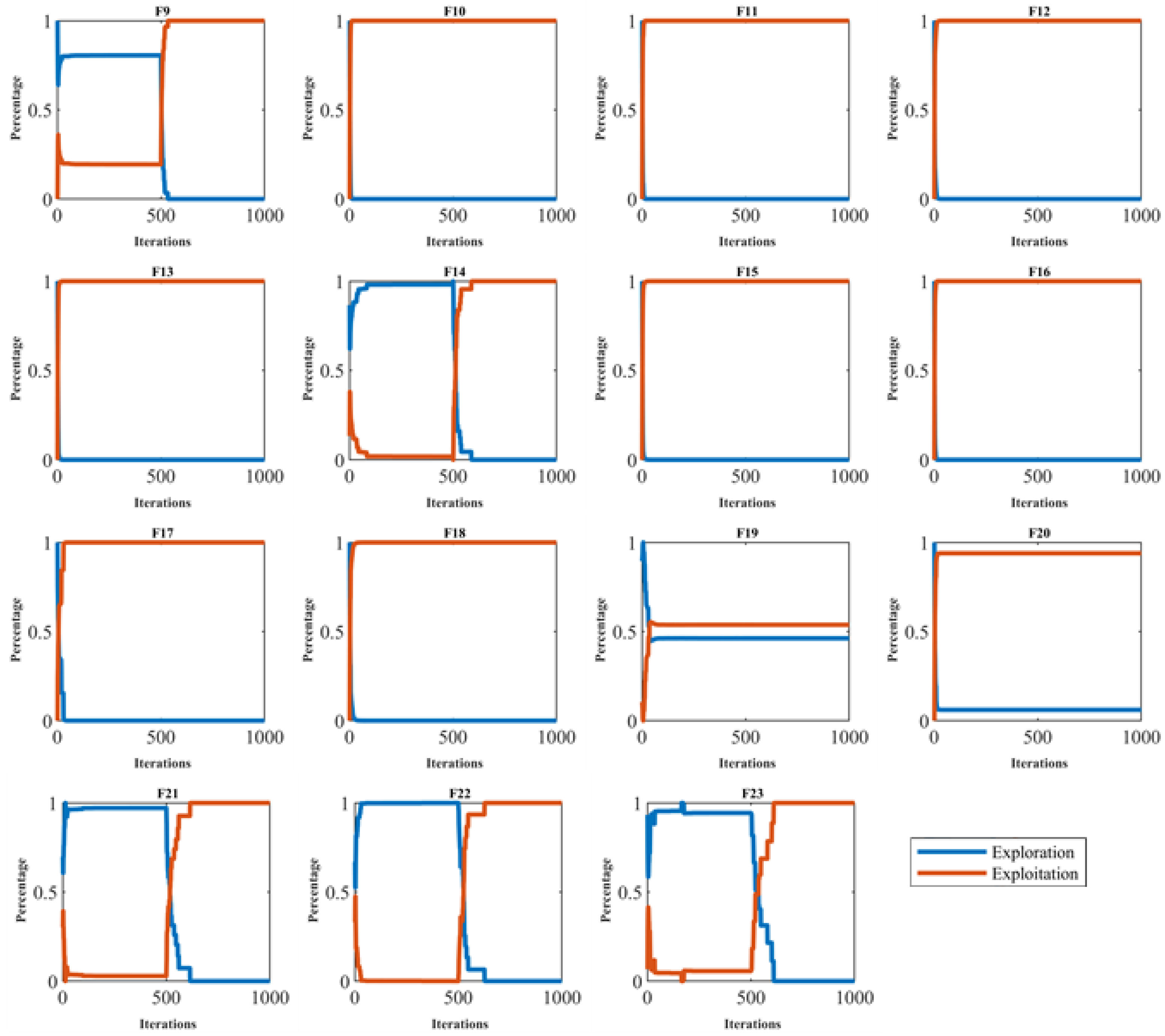
In this subsection, the analysis of population diversity, exploration, and exploitation is evaluated on twenty-three standard benchmark functions, consisting of 7 unimodal functions (F1 to F7) and 16 multimodal functions (F8 to F23). A full description of these benchmark functions is available in [78].
Figure 3 illustrates the exploration–exploitation ratio of the BOA method throughout the iteration process, offering visual support for analyzing how the algorithm balances global and local search strategies. Also, the results of the analysis of population diversity, exploration, and exploitation are reported in Table 1. The simulation results show that the BOA has favorable population diversity, where it has high values in the first iteration, while the values of this index are low in the last iteration. Also, based on the obtained results, in most cases the exploration–exploitation ratio of the BOA is close to 0.00%:100%. The findings obtained from this analysis confirm that the proposed BOA approach, by creating the appropriate population diversity during the iterations of the algorithm, provides a favorable performance in managing exploration and exploitation, and in balancing them during the search process.
4. Simulation Studies and Results
In this section, the performance of the proposed BOA approach in handling optimization tasks is evaluated.
4.1. Performance Comparison
To assess the BOA’s effectiveness in addressing optimization problems, its results were juxtaposed with those of twelve prominent metaheuristic algorithms: the GA [31], PSO [11], GSA [40], TLBO [51], MVO [42], GWO [22], WOA [26], MPA [25], TSA [17], RSA [28], AVOA [23], and WSO [21]. These twelve algorithms were selected from the numerous algorithms available in the literature. The reasons for choosing these twelve algorithms were as follows: the GA and PSO are among the first and most famous metaheuristic algorithms. The GSA, TLBO, MVO, GWO, and WOA are among the most cited metaheuristic algorithms that have been used in various optimization applications. The MPA, TSA, RSA, AVOA, and WSO approaches are among the recently published successful metaheuristic algorithms that have attracted the attention of many researchers in this short period of time. Comparing the proposed BOA approach with these twelve selected metaheuristic algorithms is a valuable comparison, after which the efficiency of the BOA will have been tested well. Table 2 outlines the control parameter values for the competing algorithms. The evaluation of the simulation results incorporates six statistical metrics: mean, best, worst, standard deviation (std), median, and rank. The mean index values were utilized for ranking the metaheuristic algorithms concerning each benchmark function.
4.2. Evaluation of the CEC 2017 Test Suite
In this section, the performance of the BOA and competing algorithms is evaluated using the CEC 2017 test suite, considering problem dimensions (number of decision variables) equal to 10, 30, 50, and 100. The CEC 2017 test suite comprises thirty benchmark functions, including three unimodal functions (C17-F1 to C17-F3), seven multimodal functions (C17-F4 to C17-F10), ten hybrid functions (C17-F11 to C17-F20), and ten composition functions (C17-F21 to C17-F30). The C17-F2 function is excluded due to its unstable behavior, as described in [79].
The results of employing the BOA approach and competing algorithms on the CEC 2017 test suite are presented in Table 3. Boxplot diagrams depicting the performance of the BOA and competing algorithms in optimizing the CEC 2017 test suite are illustrated in Figure 4. The outcomes indicate that the BOA outperformed other optimizers, ranking as the top performer for functions C17-F1, C17-F3 to C17-F21, C17-F23, C17-F24, and C17-F27 to C17-F30.
Overall, the BOA demonstrated its efficacy in providing effective solutions for the CEC 2017 test suite, showcasing a commendable ability to explore, exploit, and maintain balance throughout the search process. The simulation results establish the BOA’s superior performance over competing algorithms, securing the top rank as the best optimizer for handling the CEC 2017 test suite.
4.3. Statistical Analysis
In this section, a statistical analysis was performed on the performances of the BOA and rival algorithms to assess the significance of the BOA’s superiority from a statistical perspective. The Wilcoxon signed-rank test [80], a non-parametric test for matched or paired data, was employed for this purpose. This test helps determine whether there is a significant difference between the averages of two data samples. The results of the Wilcoxon signed-rank test, presented in Table 4, indicate instances where the BOA exhibits statistically significant superiority over the respective competing algorithms, with a p-value criterion of less than 0.05.
4.4. Discussion
In this subsection, the performance of the BOA compared to competing algorithms is discussed. The CEC 2017 test suite has different types of objective functions.
Unimodal functions C17-F1 and C17-F3 have only one main optimum (i.e., global optimum), and for that reason they are suitable criteria for measuring the exploitation ability of metaheuristic algorithms. Analysis of the simulation results shows that the proposed BOA approach, with a strong performance in local search, has superior performance against all twelve competing algorithms for handling unimodal functions. Therefore, as the first strength, the superiority of the BOA in exploitation is confirmed against competing algorithms.
Multimodal functions C17-F4 to C17-F10, in addition to the main optimum (i.e., the global optimum), also have a number of local optima, which challenge the exploration ability of metaheuristic algorithms. The findings obtained from the simulation results show that the BOA, with global search management, was able to achieve the rank of the best optimizer in the competition with the compared algorithms to handle the functions C17-F4 to C17-F10. The simulation results confirm that, as the second strength, the BOA has a better exploration ability to manage global search compared to competing algorithms.
Hybrid functions C17-F11 to C17-F20 and composition functions C17-F21 to C17-F30 are complex optimization problems that challenge the performance of metaheuristic algorithms in establishing a balance between exploration and exploitation. The simulation results of these functions show that the BOA was able to achieve the rank of the best optimizer in most of these benchmark functions, except for C17-F22, C17-F25, and C17-F26. The simulation results confirm that the BOA is highly capable of balancing exploration and exploitation when facing complex optimization problems. Therefore, as a third strength, the superiority of the BOA in balancing exploration and exploitation is confirmed compared to competing algorithms.
In addition, the statistical analysis of the Wilcoxon signed-rank test and the values obtained for the -value index, as the fourth strength, confirm that the BOA has a significant statistical superiority compared to all twelve competing algorithms.
5. BOA for Real-World Applications
In this section, the effectiveness of the proposed BOA approach in addressing real-world optimization tasks is evaluated. To this end, twenty-two constrained optimization problems from the CEC 2011 test suite, along with four engineering design problems, are utilized.
5.1. Evaluation of CEC 2011 Test Suite
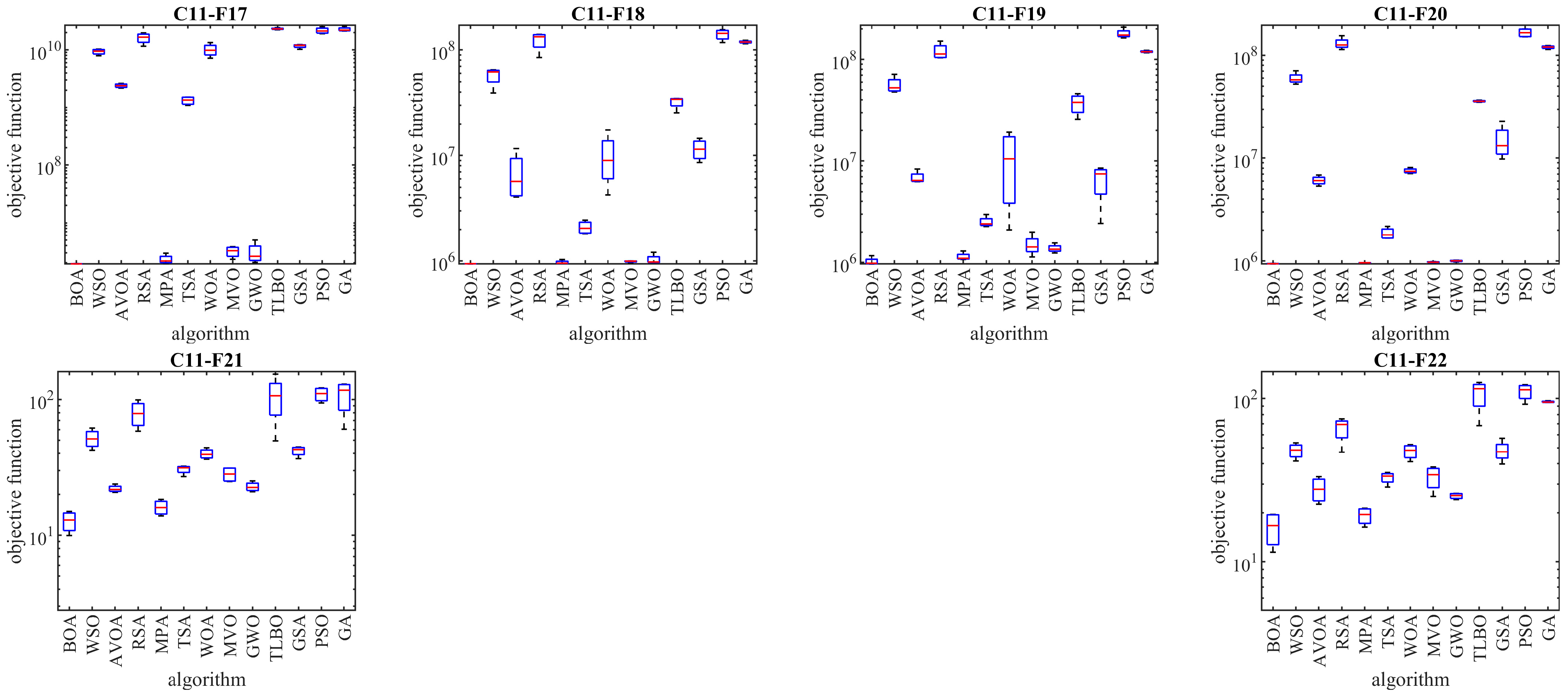
In this subsection, the performance of the BOA in optimizing the CEC 2011 test suite, which comprises twenty-two constrained optimization problems from real-world applications, is assessed. Detailed descriptions and information about the CEC 2011 test suite can be found in [81]. The results of employing the BOA and competing algorithms on the CEC 2011 test suite are presented in Table 5, and the boxplot diagrams illustrating the performance of the BOA and competing algorithms are depicted in Figure 5. The optimization outcomes highlight that the BOA effectively generated suitable solutions for this test suite, showcasing a balanced exploration and exploitation throughout the search process. Notably, the BOA emerges as the top optimizer for solving functions C11-F1 to C11-F22, demonstrating superior performance in comparison to competing algorithms. Statistical analysis, specifically the Wilcoxon signed-rank test, further validates the significant statistical superiority of the BOA in these evaluations.
5.2. Pressure Vessel Design Problem
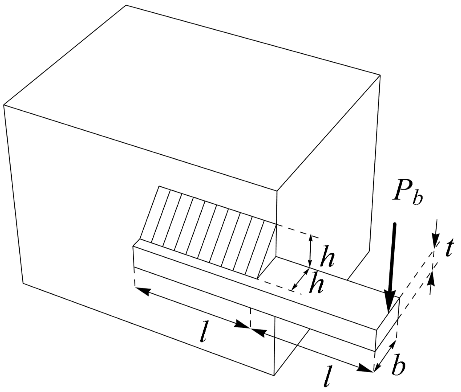
The design of the pressure vessel in engineering aims primarily to minimize construction costs, as illustrated in Figure 6. The mathematical representation of pressure vessel design is defined as follows [82]:
Consider: .
Minimize:
Subject to
with
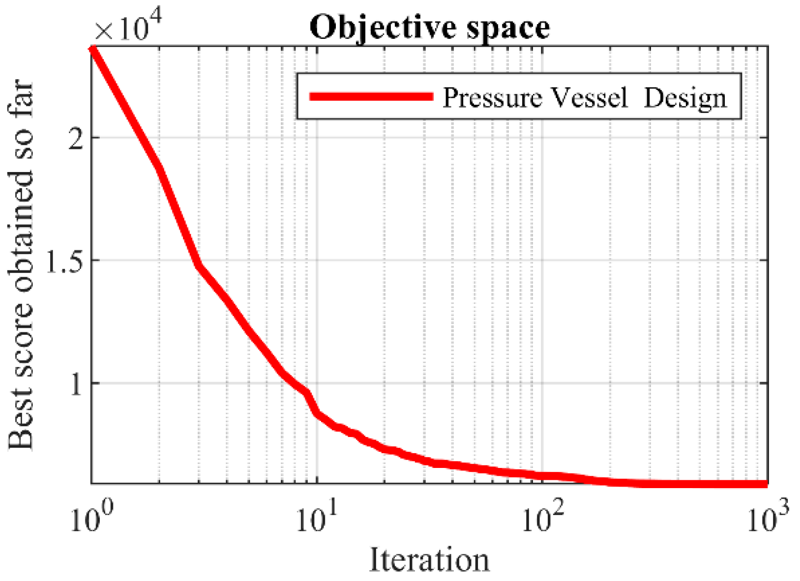
The outcomes derived from applying the BOA and rival algorithms to optimize pressure vessel design are documented in Table 6 and Table 7. According to the results, the BOA yielded the optimal solution for this design, with design variable values of ( , , ) and an objective function value of . The convergence curve of the BOA throughout the discovery of the optimal solution for pressure vessel design is depicted in Figure 7. Examination of the optimization results indicates that the BOA exhibits superior performance in addressing pressure vessel design challenges, outperforming competing algorithms.
5.3. Speed Reducer Design Problem
The design of a speed reducer is a practical engineering application focused on minimizing the weight of the speed reducer, as illustrated in Figure 8. The mathematical model for the design of the speed reducer is outlined in [83,84]:
Consider: .
Minimize: .
Subject to
with
The outcomes of implementing the BOA and competing optimizers to address the speed reducer design challenges are documented in Table 8 and Table 9. The BOA yielded the optimal solution for this design, characterized by design variable values (, ) and an objective function value of . The convergence curve, depicting the BOA’s performance in optimizing the speed reducer design, is illustrated in Figure 9. The analysis of the simulation results confirms that the BOA demonstrated more effective performance in tackling the speed reducer design compared to its competitors.
5.4. Welded Beam Design
The design of a welded beam poses a real-world engineering challenge, intending to minimize the fabrication cost of the beam, as depicted in Figure 10. The mathematical model governing the welded beam design is outlined as follows [26]:
Consider: .
Minimize: .
Subject to
where
with
The optimization outcomes for the welded beam design, utilizing the BOA and competing algorithms, are outlined in Table 10 and Table 11. The BOA yielded the optimal solution for this design, with design variable values set at (, ), resulting in an objective function value of . The convergence process of the BOA towards the optimal solution for the welded beam design is illustrated in Figure 11. The simulation results underscore the effectiveness of the BOA in addressing the welded beam design problem, showcasing superior performance compared to competing algorithms.
5.5. Tension/Compression Spring Design Problem
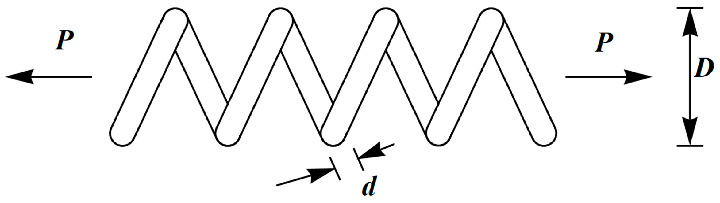
The engineering challenge in tension/compression spring design is to minimize the weight of the spring, as depicted in Figure 12. The mathematical model for tension/compression spring design is outlined as follows [26]:
Consider:
Minimize:
Subject to
with .
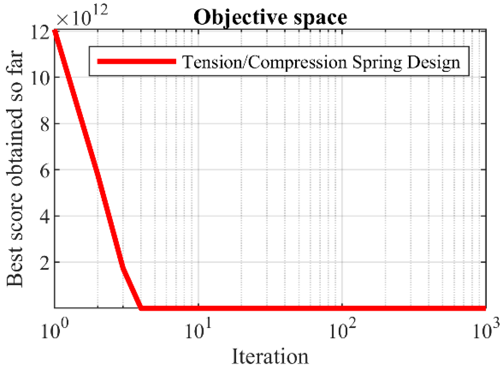
The optimization outcomes for tension/compression spring design using the BOA and competing algorithms are outlined in Table 12 and Table 13. The BOA yielded the optimal solution for this design, with design variable values of () and an objective function value of . The convergence curve depicting the BOA’s performance in optimizing the tension/compression spring design is illustrated in Figure 13. The simulation results demonstrate that the BOA exhibited superior performance compared to competing algorithms by delivering improved outcomes for tension/compression spring design.
6. Conclusions and Future Works
In this paper, motivated by the No Free Lunch (NFL) theorem, a new human-based metaheuristic algorithm called the Botox Optimization Algorithm (BOA) was introduced, mimicking the human action of Botox injections. The originality of the proposed BOA approach was confirmed based on the best knowledge obtained from the literature review, where no metaheuristic algorithm based on Botox injection modeling has been designed so far. The fundamental inspiration of the BOA is the injection of Botox into the areas of the face in order to remove defects from the face and increase facial beauty. The theory of the BOA was stated, and the various stages of its implementation were mathematically modeled based on the simulation of Botox injection. The performance of the BOA was evaluated on the CEC 2017 test suite. The optimization results showed that the BOA has a high ability to balance exploration and exploitation during the search process. To measure the quality of the BOA, the obtained results were compared with the performance of twelve well-known metaheuristic algorithms. The simulation results showed that the BOA outperformed competing algorithms by providing better results in most benchmark functions. Using statistical analysis, it was shown that the BOA has significant statistical superiority over competing algorithms. Also, the implementation of the BOA on twenty-two constrained optimization problems from the CEC 2011 test suite showed the ability of the proposed approach to handle real-world applications.
After introducing the proposed BOA approach, several research paths can be considered for further studies:
- Binary BOA: The real version of the BOA is detailed and explained thoroughly in this paper. Nonetheless, many scientific optimization issues, like feature selection, require the use of binary versions of metaheuristic algorithms for efficient optimization. Consequently, developing the binary version of the BOA (BBOA) is a notable focus of this research.
- Multi-objective BOA: Optimization problems are classified based on the number of objective functions, which are either single-objective or multi-objective. To find an optimal solution, many problems require the consideration of multiple objective functions simultaneously. Hence, exploring the potential of developing a multi-objective version of the BOA (MOBOA) to address multi-objective optimization dilemmas is another area of research highlighted in this paper.
- Hybrid BOA: Researchers have always been intrigued by the idea of merging multiple metaheuristic algorithms to leverage the strengths of each and establish a more efficient hybrid strategy. Hence, a potential future research endeavor includes crafting hybrid versions of the BOA.
- Tackle new domains: Exploring opportunities for employing the BOA in tackling practical applications and optimizing problems within various scientific fields, like robotics, renewable energy, chemical engineering, and image processing, is a focus for future research proposals.
Author Contributions
Conceptualization, P.T. and Š.H.; data curation, M.H. and Š.H.; formal analysis, M.H.; investigation, M.H. and Š.H.; methodology, P.T. and Š.H.; software, Š.H.; validation, P.T. and M.H.; visualization, M.H. and Š.H.; writing—original draft preparation, P.T. and M.H.; writing—review and editing M.H. and Š.H. All authors have read and agreed to the published version of the manuscript.
Funding
This study was supported by the specific research project FacEdu 2024 No. 2126 of the Faculty of Education, University of Hradec Králové.
Institutional Review Board Statement
Not applicable.
Informed Consent Statement
Not applicable.
Data Availability Statement
Data are contained within the article.
Acknowledgments
The authors thank the University of Hradec Králové for its support.
Conflicts of Interest
The authors declare no conflicts of interest.
References
- El-kenawy, E.-S.M.; Khodadadi, N.; Mirjalili, S.; Abdelhamid, A.A.; Eid, M.M.; Ibrahim, A. Greylag Goose Optimization: Nature-inspired optimization algorithm. Expert Syst. Appl. 2024, 238, 122147. [Google Scholar] [CrossRef]
- Singh, N.; Cao, X.; Diggavi, S.; Başar, T. Decentralized multi-task stochastic optimization with compressed communications. Automatica 2024, 159, 111363. [Google Scholar] [CrossRef]
- Liberti, L.; Kucherenko, S. Comparison of deterministic and stochastic approaches to global optimization. Int. Trans. Oper. Res. 2005, 12, 263–285. [Google Scholar] [CrossRef]
- Koc, I.; Atay, Y.; Babaoglu, I. Discrete tree seed algorithm for urban land readjustment. Eng. Appl. Artif. Intell. 2022, 112, 104783. [Google Scholar] [CrossRef]
- Trojovský, P.; Dehghani, M. Subtraction-Average-Based Optimizer: A New Swarm-Inspired Metaheuristic Algorithm for Solving Optimization Problems. Biomimetics 2023, 8, 149. [Google Scholar] [CrossRef]
- Kashan, A.H. League Championship Algorithm (LCA): An algorithm for global optimization inspired by sport championships. Appl. Soft Comput. 2014, 16, 171–200. [Google Scholar] [CrossRef]
- De Armas, J.; Lalla-Ruiz, E.; Tilahun, S.L.; Voß, S. Similarity in metaheuristics: A gentle step towards a comparison methodology. Nat. Comput. 2022, 21, 265–287. [Google Scholar] [CrossRef]
- Dehghani, M.; Montazeri, Z.; Dehghani, A.; Malik, O.P.; Morales-Menendez, R.; Dhiman, G.; Nouri, N.; Ehsanifar, A.; Guerrero, J.M.; Ramirez-Mendoza, R.A. Binary spring search algorithm for solving various optimization problems. Appl. Sci. 2021, 11, 1286. [Google Scholar] [CrossRef]
- Yang, X.-S.; Koziel, S.; Leifsson, L. Computational Optimization, Modelling and Simulation: Smart Algorithms and Better Models. Procedia Comput. Sci. 2012, 9, 852–856. [Google Scholar] [CrossRef]
- Wolpert, D.H.; Macready, W.G. No free lunch theorems for optimization. IEEE Trans. Evol. Comput. 1997, 1, 67–82. [Google Scholar] [CrossRef]
- Kennedy, J.; Eberhart, R. Particle swarm optimization. In Proceedings of the ICNN’95—International Conference on Neural Networks, Perth, WA, Australia, 27 November–1 December 1995; IEEE: Perth, WA, Australia, 1995; Volume 4, pp. 1942–1948. [Google Scholar]
- Dorigo, M.; Maniezzo, V.; Colorni, A. Ant system: Optimization by a colony of cooperating agents. IEEE Trans. Syst. Man Cybern. Part B (Cybern.) 1996, 26, 29–41. [Google Scholar] [CrossRef] [PubMed]
- Karaboga, D.; Basturk, B. Artificial bee colony (ABC) optimization algorithm for solving constrained optimization problems. In International Fuzzy Systems Association World Congress; Springer: Berlin/Heidelberg, Germany, 2007; pp. 789–798. [Google Scholar]
- Yang, X.-S. Firefly algorithm, stochastic test functions and design optimisation. Int. J. Bio-Inspired Comput. 2010, 2, 78–84. [Google Scholar] [CrossRef]
- Al-Baik, O.; Alomari, S.; Alssayed, O.; Gochhait, S.; Leonova, I.; Dutta, U.; Malik, O.P.; Montazeri, Z.; Dehghani, M. Pufferfish Optimization Algorithm: A New Bio-Inspired Metaheuristic Algorithm for Solving Optimization Problems. Biomimetics 2024, 9, 65. [Google Scholar] [CrossRef]
- Chopra, N.; Ansari, M.M. Golden Jackal Optimization: A Novel Nature-Inspired Optimizer for Engineering Applications. Expert Syst. Appl. 2022, 198, 116924. [Google Scholar] [CrossRef]
- Kaur, S.; Awasthi, L.K.; Sangal, A.L.; Dhiman, G. Tunicate Swarm Algorithm: A new bio-inspired based metaheuristic paradigm for global optimization. Eng. Appl. Artif. Intell. 2020, 90, 103541. [Google Scholar] [CrossRef]
- Dehghani, M.; Montazeri, Z.; Trojovská, E.; Trojovský, P. Coati Optimization Algorithm: A new bio-inspired metaheuristic algorithm for solving optimization problems. Knowl.-Based Syst. 2023, 259, 110011. [Google Scholar] [CrossRef]
- Braik, M.S. Chameleon Swarm Algorithm: A bio-inspired optimizer for solving engineering design problems. Expert Syst. Appl. 2021, 174, 114685. [Google Scholar] [CrossRef]
- Ghasemi, M.; Rahimnejad, A.; Hemmati, R.; Akbari, E.; Gadsden, S.A. Wild Geese Algorithm: A novel algorithm for large scale optimization based on the natural life and death of wild geese. Array 2021, 11, 100074. [Google Scholar] [CrossRef]
- Braik, M.; Hammouri, A.; Atwan, J.; Al-Betar, M.A.; Awadallah, M.A. White Shark Optimizer: A novel bio-inspired meta-heuristic algorithm for global optimization problems. Knowl.-Based Syst. 2022, 243, 108457. [Google Scholar] [CrossRef]
- Mirjalili, S.; Mirjalili, S.M.; Lewis, A. Grey Wolf Optimizer. Adv. Eng. Softw. 2014, 69, 46–61. [Google Scholar] [CrossRef]
- Abdollahzadeh, B.; Gharehchopogh, F.S.; Mirjalili, S. African vultures optimization algorithm: A new nature-inspired metaheuristic algorithm for global optimization problems. Comput. Ind. Eng. 2021, 158, 107408. [Google Scholar] [CrossRef]
- Abdel-Basset, M.; Mohamed, R.; Zidan, M.; Jameel, M.; Abouhawwash, M. Mantis Search Algorithm: A novel bio-inspired algorithm for global optimization and engineering design problems. Comput. Methods Appl. Mech. Eng. 2023, 415, 116200. [Google Scholar] [CrossRef]
- Faramarzi, A.; Heidarinejad, M.; Mirjalili, S.; Gandomi, A.H. Marine Predators Algorithm: A nature-inspired metaheuristic. Expert Syst. Appl. 2020, 152, 113377. [Google Scholar] [CrossRef]
- Mirjalili, S.; Lewis, A. The whale optimization algorithm. Adv. Eng. Softw. 2016, 95, 51–67. [Google Scholar] [CrossRef]
- Jiang, Y.; Wu, Q.; Zhu, S.; Zhang, L. Orca predation algorithm: A novel bio-inspired algorithm for global optimization problems. Expert Syst. Appl. 2022, 188, 116026. [Google Scholar] [CrossRef]
- Abualigah, L.; Abd Elaziz, M.; Sumari, P.; Geem, Z.W.; Gandomi, A.H. Reptile Search Algorithm (RSA): A nature-inspired meta-heuristic optimizer. Expert Syst. Appl. 2022, 191, 116158. [Google Scholar] [CrossRef]
- Hashim, F.A.; Houssein, E.H.; Hussain, K.; Mabrouk, M.S.; Al-Atabany, W. Honey Badger Algorithm: New metaheuristic algorithm for solving optimization problems. Math. Comput. Simul. 2022, 192, 84–110. [Google Scholar] [CrossRef]
- Dehghani, M.; Montazeri, Z.; Bektemyssova, G.; Malik, O.P.; Dhiman, G.; Ahmed, A.E.M. Kookaburra Optimization Algorithm: A New Bio-Inspired Metaheuristic Algorithm for Solving Optimization Problems. Biomimetics 2023, 8, 470. [Google Scholar] [CrossRef]
- Goldberg, D.E.; Holland, J.H. Genetic Algorithms and Machine Learning. Mach. Learn. 1988, 3, 95–99. [Google Scholar] [CrossRef]
- Storn, R.; Price, K. Differential evolution–a simple and efficient heuristic for global optimization over continuous spaces. J. Glob. Optim. 1997, 11, 341–359. [Google Scholar] [CrossRef]
- De Castro, L.N.; Timmis, J.I. Artificial immune systems as a novel soft computing paradigm. Soft Comput. 2003, 7, 526–544. [Google Scholar] [CrossRef]
- Koza, J.R.; Koza, J.R. Genetic Programming: On the Programming of Computers by Means of Natural Selection; MIT Press: Cambridge, MA, USA, 1992; Volume 1. [Google Scholar]
- Reynolds, R.G. An introduction to cultural algorithms. In Proceedings of the Third Annual Conference on Evolutionary Programming, San Diego, CA, USA, 24–26 February 1994; World Scientific Publishing: Singapore, 1994; pp. 131–139. [Google Scholar]
- Beyer, H.-G.; Schwefel, H.-P. Evolution strategies—A comprehensive introduction. Nat. Comput. 2002, 1, 3–52. [Google Scholar] [CrossRef]
- Kirkpatrick, S.; Gelatt, C.D.; Vecchi, M.P. Optimization by simulated annealing. Science 1983, 220, 671–680. [Google Scholar] [CrossRef] [PubMed]
- Dehghani, M.; Samet, H. Momentum search algorithm: A new meta-heuristic optimization algorithm inspired by momentum conservation law. SN Appl. Sci. 2020, 2, 1720. [Google Scholar] [CrossRef]
- Dehghani, M.; Montazeri, Z.; Dhiman, G.; Malik, O.; Morales-Menendez, R.; Ramirez-Mendoza, R.A.; Dehghani, A.; Guerrero, J.M.; Parra-Arroyo, L. A spring search algorithm applied to engineering optimization problems. Appl. Sci. 2020, 10, 6173. [Google Scholar] [CrossRef]
- Rashedi, E.; Nezamabadi-Pour, H.; Saryazdi, S. GSA: A gravitational search algorithm. Inf. Sci. 2009, 179, 2232–2248. [Google Scholar] [CrossRef]
- Hatamlou, A. Black hole: A new heuristic optimization approach for data clustering. Inf. Sci. 2013, 222, 175–184. [Google Scholar] [CrossRef]
- Mirjalili, S.; Mirjalili, S.M.; Hatamlou, A. Multi-verse optimizer: A nature-inspired algorithm for global optimization. Neural Comput. Appl. 2016, 27, 495–513. [Google Scholar] [CrossRef]
- Faramarzi, A.; Heidarinejad, M.; Stephens, B.; Mirjalili, S. Equilibrium optimizer: A novel optimization algorithm. Knowl.-Based Syst. 2020, 191, 105190. [Google Scholar] [CrossRef]
- Hashim, F.A.; Hussain, K.; Houssein, E.H.; Mabrouk, M.S.; Al-Atabany, W. Archimedes optimization algorithm: A new metaheuristic algorithm for solving optimization problems. Appl. Intell. 2021, 51, 1531–1551. [Google Scholar] [CrossRef]
- Hashim, F.A.; Houssein, E.H.; Mabrouk, M.S.; Al-Atabany, W.; Mirjalili, S. Henry gas solubility optimization: A novel physics-based algorithm. Future Gener. Comput. Syst. 2019, 101, 646–667. [Google Scholar] [CrossRef]
- Cuevas, E.; Oliva, D.; Zaldivar, D.; Pérez-Cisneros, M.; Sossa, H. Circle detection using electro-magnetism optimization. Inf. Sci. 2012, 182, 40–55. [Google Scholar] [CrossRef]
- Pereira, J.L.J.; Francisco, M.B.; Diniz, C.A.; Oliver, G.A.; Cunha, S.S., Jr.; Gomes, G.F. Lichtenberg algorithm: A novel hybrid physics-based meta-heuristic for global optimization. Expert Syst. Appl. 2021, 170, 114522. [Google Scholar] [CrossRef]
- Wei, Z.; Huang, C.; Wang, X.; Han, T.; Li, Y. Nuclear reaction optimization: A novel and powerful physics-based algorithm for global optimization. IEEE Access 2019, 7, 66084–66109. [Google Scholar] [CrossRef]
- Kaveh, A.; Dadras, A. A novel meta-heuristic optimization algorithm: Thermal exchange optimization. Adv. Eng. Softw. 2017, 110, 69–84. [Google Scholar] [CrossRef]
- Eskandar, H.; Sadollah, A.; Bahreininejad, A.; Hamdi, M. Water cycle algorithm–A novel metaheuristic optimization method for solving constrained engineering optimization problems. Comput. Struct. 2012, 110, 151–166. [Google Scholar] [CrossRef]
- Rao, R.V.; Savsani, V.J.; Vakharia, D. Teaching–learning-based optimization: A novel method for constrained mechanical design optimization problems. Comput.-Aided Des. 2011, 43, 303–315. [Google Scholar] [CrossRef]
- Wei, Z.; Ke, P.; Shigang, L.; Yagang, W. Special Forces Algorithm: A novel meta-heuristic method for global optimization. Math. Comput. Simul. 2023, 213, 394–417. [Google Scholar]
- Askari, Q.; Younas, I.; Saeed, M. Political Optimizer: A novel socio-inspired meta-heuristic for global optimization. Knowl.-Based Syst. 2020, 195, 105709. [Google Scholar] [CrossRef]
- Trojovská, E.; Dehghani, M. A new human-based metahurestic optimization method based on mimicking cooking training. Sci. Rep. 2022, 12, 14861. [Google Scholar] [CrossRef]
- Al-Betar, M.A.; Alyasseri, Z.A.A.; Awadallah, M.A.; Abu Doush, I. Coronavirus herd immunity optimizer (CHIO). Neural Comput. Appl. 2021, 33, 5011–5042. [Google Scholar] [CrossRef]
- Dehghani, M.; Mardaneh, M.; Guerrero, J.M.; Malik, O.P.; Ramirez-Mendoza, R.A.; Matas, J.; Vasquez, J.C.; Parra-Arroyo, L. A new “Doctor and Patient” optimization algorithm: An application to energy commitment problem. Appl. Sci. 2020, 10, 5791. [Google Scholar] [CrossRef]
- Ayyarao, T.L.; RamaKrishna, N.; Elavarasam, R.M.; Polumahanthi, N.; Rambabu, M.; Saini, G.; Khan, B.; Alatas, B. War Strategy Optimization Algorithm: A New Effective Metaheuristic Algorithm for Global Optimization. IEEE Access 2022, 10, 25073–25105. [Google Scholar] [CrossRef]
- Trojovský, P.; Dehghani, M. A new optimization algorithm based on mimicking the voting process for leader selection. PeerJ Comput. Sci. 2022, 8, e976. [Google Scholar] [CrossRef]
- Mohamed, A.W.; Hadi, A.A.; Mohamed, A.K. Gaining-sharing knowledge based algorithm for solving optimization problems: A novel nature-inspired algorithm. Int. J. Mach. Learn. Cybern. 2020, 11, 1501–1529. [Google Scholar] [CrossRef]
- Dehghani, M.; Mardaneh, M.; Malik, O. FOA: ‘Following’ Optimization Algorithm for solving Power engineering optimization problems. J. Oper. Autom. Power Eng. 2020, 8, 57–64. [Google Scholar]
- Dehghani, M.; Trojovská, E.; Zuščák, T. A new human-inspired metaheuristic algorithm for solving optimization problems based on mimicking sewing training. Sci. Rep. 2022, 12, 17387. [Google Scholar] [CrossRef] [PubMed]
- Braik, M.; Ryalat, M.H.; Al-Zoubi, H. A novel meta-heuristic algorithm for solving numerical optimization problems: Ali Baba and the forty thieves. Neural Comput. Appl. 2022, 34, 409–455. [Google Scholar] [CrossRef]
- Dehghani, M.; Mardaneh, M.; Guerrero, J.M.; Malik, O.; Kumar, V. Football game based optimization: An application to solve energy commitment problem. Int. J. Intell. Eng. Syst. 2020, 13, 514–523. [Google Scholar] [CrossRef]
- Moghdani, R.; Salimifard, K. Volleyball premier league algorithm. Appl. Soft Comput. 2018, 64, 161–185. [Google Scholar] [CrossRef]
- Dehghani, M.; Montazeri, Z.; Saremi, S.; Dehghani, A.; Malik, O.P.; Al-Haddad, K.; Guerrero, J.M. HOGO: Hide objects game optimization. Int. J. Intell. Eng. Syst. 2020, 13, 216–225. [Google Scholar] [CrossRef]
- Dehghani, M.; Montazeri, Z.; Givi, H.; Guerrero, J.M.; Dhiman, G. Darts game optimizer: A new optimization technique based on darts game. Int. J. Intell. Eng. Syst. 2020, 13, 286–294. [Google Scholar] [CrossRef]
- Dehghani, M.; Montazeri, Z.; Malik, O.P.; Ehsanifar, A.; Dehghani, A. OSA: Orientation search algorithm. International Journal of Industrial Electronics. Control. Optim. 2019, 2, 99–112. [Google Scholar]
- Dehghani, M.; Montazeri, Z.; Malik, O.P. DGO: Dice game optimizer. Gazi Univ. J. Sci. 2019, 32, 871–882. [Google Scholar] [CrossRef]
- Doumari, S.A.; Givi, H.; Dehghani, M.; Malik, O.P. Ring Toss Game-Based Optimization Algorithm for Solving Various Optimization Problems. Int. J. Intell. Eng. Syst. 2021, 14, 545–554. [Google Scholar] [CrossRef]
- Zeidabadi, F.A.; Dehghani, M. POA: Puzzle Optimization Algorithm. Int. J. Intell. Eng. Syst. 2022, 15, 273–281. [Google Scholar]
- Yao, L.; Yuan, P.; Tsai, C.-Y.; Zhang, T.; Lu, Y.; Ding, S. ESO: An enhanced snake optimizer for real-world engineering problems. Expert Syst. Appl. 2023, 230, 120594. [Google Scholar] [CrossRef]
- Hong, J.; Shen, B.; Xue, J.; Pan, A. A vector-encirclement-model-based sparrow search algorithm for engineering optimization and numerical optimization problems. Appl. Soft Comput. 2022, 131, 109777. [Google Scholar] [CrossRef]
- Wei, F.; Zhang, Y.; Li, J. Multi-strategy-based adaptive sine cosine algorithm for engineering optimization problems. Expert Syst. Appl. 2024, 248, 123444. [Google Scholar] [CrossRef]
- Dressler, D.; Benecke, R. Pharmacology of therapeutic botulinum toxin preparations. Disabil. Rehabil. 2007, 29, 1761–1768. [Google Scholar] [CrossRef]
- Blasi, J.; Chapman, E.R.; Link, E.; Binz, T.; Yamasaki, S.; Camilli, P.D.; Südhof, T.C.; Niemann, H.; Jahn, R. Botulinum neurotoxin A selectively cleaves the synaptic protein SNAP-25. Nature 1993, 365, 160–163. [Google Scholar] [CrossRef] [PubMed]
- Small, R. Botulinum toxin injection for facial wrinkles. Am. Fam. Physician 2014, 90, 168–175. [Google Scholar] [PubMed]
- Pant, M.; Radha, T.; Singh, V.P. A simple diversity guided particle swarm optimization. In Proceedings of the 2007 IEEE Congress on Evolutionary Computation, Singapore, 25–28 September 2007; IEEE: Piscataway, NJ, USA, 2007; pp. 3294–3299. [Google Scholar]
- Yao, X.; Liu, Y.; Lin, G. Evolutionary programming made faster. IEEE Trans. Evol. Comput. 1999, 3, 82–102. [Google Scholar]
- Awad, N.; Ali, M.; Liang, J.; Qu, B.; Suganthan, P.; Definitions, P. Evaluation criteria for the CEC 2017 special session and competition on single objective real-parameter numerical optimization. Technol. Rep. 2016. [Google Scholar]
- Wilcoxon, F. Individual comparisons by ranking methods. In Breakthroughs in Statistics; Springer: Berlin/Heidelberg, Germany, 1992; pp. 196–202. [Google Scholar]
- Das, S.; Suganthan, P.N. Problem Definitions and Evaluation Criteria for CEC 2011 Competition on Testing Evolutionary Algorithms on Real World Optimization Problems; Jadavpur University: Kolkata, India; Nanyang Technological University: Singapore, 2010; pp. 341–359. [Google Scholar]
- Kannan, B.; Kramer, S.N. An augmented Lagrange multiplier based method for mixed integer discrete continuous optimization and its applications to mechanical design. J. Mech. Des. 1994, 116, 405–411. [Google Scholar] [CrossRef]
- Gandomi, A.H.; Yang, X.-S. Benchmark problems in structural optimization. In Computational Optimization, Methods and Algorithms; Springer: Berlin/Heidelberg, Germany, 2011; pp. 259–281. [Google Scholar]
- Mezura-Montes, E.; Coello, C.A.C. Useful infeasible solutions in engineering optimization with evolutionary algorithms. In Proceedings of the Mexican International Conference on Artificial Intelligence, Monterrey, Mexico, 14–18 November 2005; Springer: Berlin/Heidelberg, Germany, 2005; pp. 652–662. [Google Scholar]
Figure 1.
Schematic diagram of the Botox injection and the proposed BOA.

Figure 2.
Flowchart of the BOA.

Figure 3.
Exploration and exploitation of the BOA.


Figure 4.
Boxplot representations illustrating the performances of the BOA and rival algorithms on the CEC 2017 test suite.
Figure 4.
Boxplot representations illustrating the performances of the BOA and rival algorithms on the CEC 2017 test suite.


Figure 5.
Boxplot diagrams of the BOA and competing algorithms’ performances on the CEC 2011 test suite.
Figure 5.
Boxplot diagrams of the BOA and competing algorithms’ performances on the CEC 2011 test suite.


Figure 6.
Schematic of pressure vessel design. The thickness of the shell is , the thickness of the head is , the length of cylindrical shell is , and the inner radius is .
Figure 6.
Schematic of pressure vessel design. The thickness of the shell is , the thickness of the head is , the length of cylindrical shell is , and the inner radius is .

Figure 7.
The BOA’s performance convergence curve on pressure vessel design.

Figure 8.
Schematic of speed reducer design. The face width is , the number of teeth on the pinion is , the module of teeth is , the length of the second shaft between bearings is , the length of the first shaft between bearings is , the second shaft’s diameter is , and the first shaft’s diameter is .

Figure 9.
The BOA’s performance convergence curve on speed reducer design.

Figure 10.
Schematic of welded beam design. The bar height is , the weld thickness is , the thickness of bar is , and the length of clamped bar is .
Figure 10.
Schematic of welded beam design. The bar height is , the weld thickness is , the thickness of bar is , and the length of clamped bar is .

Figure 11.
The BOA’s performance convergence curve on welded beam design.

Figure 12.
Schematic of tension/compression spring design. The wire’s diameter is , the number of active coils is , and the mean coil’s diameter is .
Figure 12.
Schematic of tension/compression spring design. The wire’s diameter is , the number of active coils is , and the mean coil’s diameter is .

Figure 13.
The BOA’s performance convergence curve on tension/compression spring design.


Table 1.
Population diversity, exploration, and exploitation percentage results.
| Function Name | Exploration | Exploitation | Diversity | |
|---|---|---|---|---|
| First Iteration | Last Iteration | |||
| F1 | 0 | 1 | 140.5903 | 0 |
| F2 | 0 | 1 | 10.94242 | 0 |
| F3 | 0 | 1 | 252.3905 | 0 |
| F4 | 0 | 1 | 128.8175 | 0 |
| F5 | 0 | 1 | 44.92006 | 0 |
| F6 | 0.012744 | 0.987256 | 114.0171 | 1.453073 |
| F7 | 0.049372 | 0.950628 | 1.518403 | 0.074966 |
| F8 | 5.84E-10 | 1 | 1230.61 | 1.19E-06 |
| F9 | 4.76E-10 | 1 | 9.555822 | 4.55E-09 |
| F10 | 1.8E-17 | 1 | 50.32814 | 9.04E-16 |
| F11 | 3.7E-11 | 1 | 885.0467 | 3.27E-08 |
| F12 | 0 | 1 | 61.45876 | 0 |
| F13 | 0 | 1 | 77.58755 | 0 |
| F14 | 2.02E-08 | 1 | 23.65722 | 4.77E-07 |
| F15 | 5.93E-11 | 1 | 4.048837 | 2.4E-10 |
| F16 | 0.082221 | 0.917779 | 1.61018 | 0.13239 |
| F17 | 6.68E-10 | 1 | 4.961695 | 3.31E-09 |
| F18 | 0.068118 | 0.931882 | 0.757968 | 0.051631 |
| F19 | 0.245007 | 0.754993 | 0.378584 | 0.118559 |
| F20 | 0.054777 | 0.945223 | 0.441119 | 0.024163 |
| F21 | 1.95E-10 | 1 | 3.149125 | 7.25E-10 |
| F22 | 1.36E-10 | 1 | 3.505294 | 6.63E-10 |
| F23 | 9.32E-11 | 1 | 4.347473 | 4.27E-10 |
Table 2.
Control parameters’ values.
| Algorithm | Parameter | Value |
|---|---|---|
| GA | ||
| Type | Real coded | |
| Selection | Roulette wheel (proportionate) | |
| Crossover | Whole arithmetic (, ) | |
| Mutation | Gaussian () | |
| PSO | ||
| Topology | Fully connected | |
| Cognitive and social constant | () | |
| Inertia weight | Linear reduction from 0.9 to 0.1 | |
| Velocity limit | 10% of dimension range | |
| GSA | ||
| Alpha, , , | 20, 100, 2, 1 | |
| TLBO | ||
| : Teaching factor | ||
| Random number | rand is a random number from | |
| GWO | ||
| Convergence parameter () | : Linear reduction from 2 to 0. | |
| MVO | ||
| Wormhole Existence Probability (WEP) | and . | |
| Exploitation accuracy over the iterations () | . | |
| WOA | ||
| Convergence parameter () | : Linear reduction from 2 to 0. | |
| r is a random vector in ; | ||
| l is a random number in | ||
| TSA | ||
| 1, 4 | ||
| Random numbers lie in the interval | ||
| MPA | ||
| Constant number | ||
| Random vector | R is a vector of uniform random numbers in | |
| Fish Aggregating Devices (FADs) | ||
| Binary vector | or 1 | |
| RSA | ||
| Sensitive parameter | ||
| Sensitive parameter | ||
| Evolutionary Sense (ES) | ES: Randomly decreasing values between 2 and −2 | |
| AVOA | ||
| 0.8, 0.2 | ||
| 2.5 | ||
| 0.6, 0.4, 0.6 | ||
| WSO | ||
| 0.07, 0.75 | ||
| , | 4.125, 6.25, 100, 0.0005 |
Table 3.
Optimization results of the CEC 2017 test suite.
| BOA | WSO | AVOA | RSA | MPA | TSA | WOA | MVO | GWO | TLBO | GSA | PSO | GA | ||
|---|---|---|---|---|---|---|---|---|---|---|---|---|---|---|
| C17-F1 | Mean | 100 | 5.46E+09 | 3848.625 | 1.02E+10 | 35,331,826 | 1.74E+09 | 6,458,531 | 7530.831 | 88,328,653 | 1.47E+08 | 747.4345 | 3148.604 | 11,867,816 |
| Best | 100 | 4.59E+09 | 115.6391 | 8.84E+09 | 11,218.07 | 3.73E+08 | 4,702,752 | 4790.099 | 27,833.68 | 65,653,192 | 100.0193 | 345.9935 | 6,145,607 | |
| Worst | 100 | 6.85E+09 | 11,928.77 | 1.22E+10 | 1.28E+08 | 3.8E+09 | 8,503,451 | 11,096.78 | 3.21E+08 | 3.56E+08 | 1792.381 | 9323.402 | 17,037,274 | |
| Std | 0 | 1.07E+09 | 6005.345 | 1.64E+09 | 67,796,179 | 1.66E+09 | 1,750,529 | 3215.353 | 1.69E+08 | 1.52E+08 | 796.8781 | 4524.035 | 4,954,471 | |
| Median | 100 | 5.21E+09 | 1675.046 | 9.94E+09 | 6,476,105 | 1.4E+09 | 6,313,960 | 7118.225 | 16,188,754 | 84,181,901 | 548.6691 | 1462.51 | 12,144,191 | |
| Rank | 1 | 12 | 4 | 13 | 8 | 11 | 6 | 5 | 9 | 10 | 2 | 3 | 7 | |
| C17-F3 | Mean | 300 | 7591.42 | 301.8957 | 9658.226 | 1408.746 | 11,214.42 | 1731.412 | 300.0547 | 3071.866 | 726.7343 | 10,268.87 | 300 | 14,789.2 |
| Best | 300 | 4113.783 | 300 | 5207.518 | 791.8459 | 4270.307 | 619.6359 | 300.0127 | 1529.615 | 471.4213 | 6461.812 | 300 | 4354.021 | |
| Worst | 300 | 10,174.7 | 304.0548 | 12,922.2 | 2537.378 | 15,855.2 | 3333.866 | 300.1245 | 5893.445 | 893.5147 | 13,957.47 | 300 | 23,376.32 | |
| Std | 0 | 2896.121 | 2.393662 | 3838.968 | 876.4573 | 5353.91 | 1391.667 | 0.05345 | 2191.143 | 201.3742 | 3364.571 | 5.05E-14 | 10,814.33 | |
| Median | 300 | 8038.595 | 301.764 | 10,251.59 | 1152.881 | 12,366.08 | 1486.072 | 300.0407 | 2432.202 | 771.0005 | 10,328.09 | 300 | 15,713.23 | |
| Rank | 1 | 9 | 4 | 10 | 6 | 12 | 7 | 3 | 8 | 5 | 11 | 2 | 13 | |
| C17-F4 | Mean | 400 | 919.2957 | 404.7605 | 1352.77 | 406.7394 | 576.7582 | 425.1975 | 403.341 | 411.7605 | 409.1884 | 404.5619 | 420.3519 | 414.7475 |
| Best | 400 | 672.5461 | 401.2436 | 845.7611 | 402.4511 | 477.9916 | 406.4543 | 401.5971 | 406.1014 | 408.4021 | 403.5684 | 400.1059 | 411.7011 | |
| Worst | 400 | 1142.743 | 406.5393 | 1849.389 | 411.4014 | 692.0754 | 473.6998 | 404.9048 | 428.4155 | 409.6849 | 406.0879 | 470.5109 | 418.4747 | |
| Std | 0 | 229.2926 | 2.715361 | 466.2296 | 4.804772 | 114.2038 | 35.29756 | 1.871726 | 12.08414 | 0.598616 | 1.257481 | 36.76729 | 3.226255 | |
| Median | 400 | 930.9465 | 405.6296 | 1357.964 | 406.5525 | 568.4828 | 410.3179 | 403.431 | 406.2626 | 409.3334 | 404.2956 | 405.3954 | 414.407 | |
| Rank | 1 | 12 | 4 | 13 | 5 | 11 | 10 | 2 | 7 | 6 | 3 | 9 | 8 | |
| C17-F5 | Mean | 501.2464 | 562.2888 | 544.5598 | 573.6638 | 513.037 | 565.1128 | 541.4479 | 523.9769 | 513.1801 | 534.4525 | 554.4872 | 528.2287 | 528.3418 |
| Best | 500.9951 | 547.4308 | 527.1499 | 558.8475 | 508.4371 | 543.7341 | 523.7238 | 510.3406 | 508.6157 | 528.9014 | 549.5681 | 511.27 | 523.5807 | |
| Worst | 501.9917 | 572.2487 | 563.5795 | 588.8477 | 518.2122 | 597.5197 | 577.7367 | 538.4222 | 520.5555 | 538.0275 | 566.3814 | 552.3704 | 534.175 | |
| Std | 0.540776 | 12.11165 | 20.81022 | 18.12589 | 5.591417 | 25.96825 | 27.5346 | 12.761 | 5.604703 | 4.364766 | 8.746105 | 20.64316 | 5.206467 | |
| Median | 500.9993 | 564.7379 | 543.7549 | 573.48 | 512.7494 | 559.5987 | 532.1655 | 523.5724 | 511.7746 | 535.4404 | 550.9996 | 524.6372 | 527.8058 | |
| Rank | 1 | 11 | 9 | 13 | 2 | 12 | 8 | 4 | 3 | 7 | 10 | 5 | 6 | |
| C17-F6 | Mean | 600 | 632.7824 | 617.595 | 641.3535 | 601.2128 | 625.225 | 623.5356 | 602.184 | 601.1449 | 606.9718 | 617.4791 | 607.548 | 610.4234 |
| Best | 600 | 628.194 | 616.5747 | 638.0899 | 600.7222 | 615.3143 | 607.646 | 600.4796 | 600.6055 | 604.8344 | 602.9627 | 601.3762 | 607.0149 | |
| Worst | 600 | 637.5379 | 620.1871 | 645.6746 | 602.4363 | 641.0634 | 645.9187 | 604.3818 | 601.7463 | 610.3045 | 636.7176 | 619.5657 | 614.7356 | |
| Std | 0 | 4.413003 | 1.88613 | 3.709445 | 0.889975 | 12.08883 | 17.5391 | 1.908475 | 0.513952 | 2.714097 | 16.99487 | 8.979175 | 3.72455 | |
| Median | 600 | 632.699 | 616.8091 | 640.8248 | 600.8464 | 622.2611 | 620.2889 | 601.9373 | 601.1139 | 606.3741 | 615.1181 | 604.6251 | 609.9715 | |
| Rank | 1 | 12 | 9 | 13 | 3 | 11 | 10 | 4 | 2 | 5 | 8 | 6 | 7 | |
| C17-F7 | Mean | 711.1267 | 797.8688 | 766.4303 | 805.8543 | 724.8556 | 830.358 | 762.9002 | 731.196 | 726.2532 | 752.71 | 717.2159 | 733.0903 | 737.2869 |
| Best | 710.6726 | 780.6589 | 744.4304 | 792.4154 | 720.5783 | 789.6269 | 751.7383 | 717.2818 | 717.5639 | 748.1129 | 714.8806 | 725.8012 | 726.7599 | |
| Worst | 711.7995 | 809.4588 | 794.6393 | 818.7295 | 729.351 | 872.5061 | 792.8006 | 750.7791 | 744.0606 | 760.9719 | 721.0193 | 744.8461 | 741.9507 | |
| Std | 0.557384 | 13.284 | 25.13695 | 13.44422 | 4.022787 | 39.18582 | 21.75715 | 15.33828 | 13.2473 | 6.2627 | 2.892038 | 9.451487 | 7.758608 | |
| Median | 711.0174 | 800.6788 | 763.3257 | 806.1362 | 724.7466 | 829.6494 | 753.531 | 728.3615 | 721.6942 | 750.8777 | 716.4818 | 730.8569 | 740.2185 | |
| Rank | 1 | 11 | 10 | 12 | 3 | 13 | 9 | 5 | 4 | 8 | 2 | 6 | 7 | |
| C17-F8 | Mean | 801.4928 | 848.1769 | 831.617 | 854.5622 | 812.8571 | 849.0636 | 836.9437 | 812.0059 | 816.0909 | 838.313 | 820.1744 | 823.1267 | 817.0493 |
| Best | 800.995 | 842.8959 | 820.611 | 843.1502 | 808.9812 | 832.594 | 818.8766 | 807.536 | 810.6855 | 831.2975 | 812.2041 | 815.9405 | 813.0058 | |
| Worst | 801.9912 | 854.7381 | 847.6997 | 859.9005 | 815.0312 | 868.6915 | 849.3401 | 816.8821 | 821.1703 | 846.4472 | 828.0838 | 829.679 | 824.9831 | |
| Std | 0.625636 | 6.701009 | 12.45098 | 8.409374 | 3.041009 | 17.47606 | 14.23885 | 4.180792 | 4.773722 | 8.432783 | 7.354204 | 7.407172 | 5.86208 | |
| Median | 801.4926 | 847.5368 | 829.0787 | 857.599 | 813.708 | 847.4845 | 839.779 | 811.8029 | 816.2538 | 837.7536 | 820.2048 | 823.4438 | 815.1042 | |
| Rank | 1 | 11 | 8 | 13 | 3 | 12 | 9 | 2 | 4 | 10 | 6 | 7 | 5 | |
| C17-F9 | Mean | 900 | 1430.961 | 1192.849 | 1476.617 | 905.2837 | 1388.608 | 1383.102 | 900.8146 | 912.1313 | 912.0221 | 900 | 904.3122 | 905.1958 |
| Best | 900 | 1276.126 | 954.6109 | 1379.243 | 900.3329 | 1172.43 | 1076.987 | 900.0011 | 900.5827 | 907.3517 | 900 | 900.9142 | 902.8443 | |
| Worst | 900 | 1573.852 | 1673.688 | 1616.361 | 913.5628 | 1681.601 | 1668.813 | 903.166 | 933.6785 | 920.3352 | 900 | 912.5228 | 909.2282 | |
| Std | 0 | 140.1941 | 362.6238 | 109.8787 | 6.480782 | 239.779 | 271.1443 | 1.706569 | 16.89776 | 6.209908 | 0 | 6.03293 | 3.14228 | |
| Median | 900 | 1436.932 | 1071.549 | 1455.432 | 903.6196 | 1350.2 | 1393.304 | 900.0457 | 907.1319 | 910.2007 | 900 | 901.9059 | 904.3554 | |
| Rank | 1 | 11 | 8 | 12 | 5 | 10 | 9 | 2 | 7 | 6 | 1 | 3 | 4 | |
| C17-F10 | Mean | 1006.179 | 2311.834 | 1782.706 | 2588.899 | 1519.782 | 2039.361 | 2031.708 | 1785.695 | 1729.938 | 2179.736 | 2286.565 | 1951.968 | 1720.13 |
| Best | 1000.284 | 2010.815 | 1486.512 | 2416.757 | 1393.592 | 1762.237 | 1452.075 | 1458.762 | 1542.197 | 1786.243 | 2004.951 | 1563.92 | 1417.123 | |
| Worst | 1012.668 | 2456.623 | 2423.148 | 2951.232 | 1595.402 | 2293.271 | 2559.74 | 2290.911 | 1998.556 | 2469.964 | 2393.264 | 2360.873 | 2118.219 | |
| Std | 7.244311 | 225.7849 | 478.7803 | 270.7973 | 103.4757 | 304.9995 | 582.7437 | 438.7957 | 211.0887 | 316.3582 | 204.7244 | 356.2546 | 327.1839 | |
| Median | 1005.882 | 2389.949 | 1610.583 | 2493.804 | 1545.066 | 2050.967 | 2057.508 | 1696.554 | 1689.498 | 2231.369 | 2374.023 | 1941.539 | 1672.588 | |
| Rank | 1 | 12 | 5 | 13 | 2 | 9 | 8 | 6 | 4 | 10 | 11 | 7 | 3 | |
| C17-F11 | Mean | 1100 | 3442.37 | 1148.775 | 4000.383 | 1127.198 | 5484.031 | 1151.243 | 1127.661 | 1155.582 | 1151.197 | 1139.413 | 1143.772 | 2389.968 |
| Best | 1100 | 2188.762 | 1117.145 | 1460.621 | 1113.275 | 5334.971 | 1113.032 | 1105.577 | 1121.743 | 1138.044 | 1119.755 | 1132.432 | 1115.129 | |
| Worst | 1100 | 4665.813 | 1202.357 | 6508.91 | 1159.111 | 5565.816 | 1173.513 | 1149.188 | 1229.094 | 1172.713 | 1169 | 1165.388 | 6006.61 | |
| Std | 0 | 1210.189 | 40.81842 | 2469.216 | 23.5556 | 111.6604 | 30.39483 | 23.71355 | 54.46268 | 16.28689 | 22.87379 | 16.15173 | 2624.636 | |
| Median | 1100 | 3457.454 | 1137.8 | 4016 | 1118.203 | 5517.668 | 1159.213 | 1127.94 | 1135.746 | 1147.016 | 1134.448 | 1138.634 | 1219.067 | |
| Rank | 1 | 11 | 6 | 12 | 2 | 13 | 8 | 3 | 9 | 7 | 4 | 5 | 10 | |
| C17-F12 | Mean | 1352.959 | 3.57E+08 | 1,109,704 | 7.11E+08 | 572,257.8 | 1,048,288 | 2,373,547 | 1,037,633 | 1,427,055 | 5,094,522 | 1,028,834 | 8145.64 | 610,018.9 |
| Best | 1318.646 | 80,192,749 | 358,948.9 | 1.58E+08 | 20,015.65 | 543,606.5 | 173,159.8 | 8892.711 | 45,801.15 | 1,363,349 | 478,453.6 | 2528.033 | 176,684.6 | |
| Worst | 1438.176 | 6.23E+08 | 2,012,446 | 1.24E+09 | 895,571.3 | 1,286,990 | 3,937,641 | 3,259,364 | 2,233,764 | 9,018,848 | 1,739,931 | 14,021.19 | 1,076,854 | |
| Std | 62.35801 | 2.98E+08 | 841,688.2 | 5.98E+08 | 419,783.3 | 381,500.6 | 1,904,475 | 1,634,093 | 1,049,512 | 4,413,129 | 581,137.5 | 5698.792 | 402,260.9 | |
| Median | 1327.506 | 3.62E+08 | 1,033,710 | 7.22E+08 | 686,722.1 | 1,181,277 | 2,691,694 | 441,138.1 | 1,714,326 | 4,997,944 | 948,475.7 | 8016.671 | 593,268.4 | |
| Rank | 1 | 12 | 8 | 13 | 3 | 7 | 10 | 6 | 9 | 11 | 5 | 2 | 4 | |
| C17-F13 | Mean | 1305.324 | 17,335,628 | 18,471.94 | 34,661,545 | 5468.243 | 12,831.35 | 7630.328 | 6772.94 | 10,372.78 | 16,852.54 | 10,143.18 | 6664.754 | 54,887.32 |
| Best | 1303.114 | 1,445,254 | 2734.676 | 2,877,682 | 3740.627 | 7639.26 | 3297.206 | 1386.726 | 6550.028 | 15,912.77 | 5078.007 | 2387.751 | 8603.051 | |
| Worst | 1308.508 | 57,542,238 | 31,658.65 | 1.15E+08 | 6689.907 | 20,335.57 | 15,267.01 | 12,470.28 | 14,494.81 | 19,148.28 | 14,291.03 | 16,841.17 | 181,516.7 | |
| Std | 2.473462 | 29,234,423 | 16,273.34 | 58,465,686 | 1530.879 | 5963.582 | 5938.403 | 6247.984 | 3543.419 | 1681.501 | 4237.976 | 7465.241 | 91,927.81 | |
| Median | 1304.837 | 5,177,510 | 19,747.21 | 10,349,214 | 5721.218 | 11,675.29 | 5978.549 | 6617.376 | 10,223.15 | 16,174.55 | 10,601.85 | 3715.048 | 14,714.78 | |
| Rank | 1 | 12 | 10 | 13 | 2 | 8 | 5 | 4 | 7 | 9 | 6 | 3 | 11 | |
| C17-F14 | Mean | 1400.746 | 3828.915 | 2027.645 | 5383.694 | 1945.167 | 3405.109 | 1520.154 | 1573.519 | 2355.252 | 1592.631 | 5604.306 | 3010.581 | 13,069.42 |
| Best | 1400 | 3170.6 | 1681.663 | 4711.086 | 1435.363 | 1488.751 | 1482.596 | 1423.322 | 1462.902 | 1517.224 | 4631.803 | 1432.831 | 3748.476 | |
| Worst | 1400.995 | 5066.928 | 2841.448 | 6948.68 | 2917.489 | 5622.496 | 1560.295 | 1999.133 | 4996.706 | 1623.198 | 7611.074 | 6894.737 | 26,056.87 | |
| Std | 0.541408 | 945.4187 | 594.8446 | 1143.911 | 756.5397 | 2393.086 | 43.20222 | 308.8712 | 1916.5 | 54.97335 | 1519.18 | 2840.855 | 10,284.68 | |
| Median | 1400.995 | 3539.066 | 1793.735 | 4937.505 | 1713.908 | 3254.594 | 1518.862 | 1435.81 | 1480.701 | 1615.05 | 5087.174 | 1857.377 | 11,236.18 | |
| Rank | 1 | 10 | 6 | 11 | 5 | 9 | 2 | 3 | 7 | 4 | 12 | 8 | 13 | |
| C17-F15 | Mean | 1500.331 | 10,283.95 | 5333.31 | 13,989.15 | 3998.841 | 7053.662 | 6262.146 | 1542.234 | 5854.355 | 1711.148 | 24,088.27 | 9066.744 | 4578.338 |
| Best | 1500.001 | 3259.43 | 2077.801 | 2745.559 | 3239.281 | 2327.191 | 2019.265 | 1526.157 | 3589.383 | 1584.901 | 11,316.55 | 2884.332 | 1894.197 | |
| Worst | 1500.5 | 17,559.48 | 12,730.21 | 30,627 | 4923.526 | 12,648.29 | 13,558.05 | 1554.385 | 6950.016 | 1801.652 | 36,159.61 | 14,917.69 | 8074.57 | |
| Std | 0.256213 | 6701.944 | 5408.362 | 13,248.87 | 760.3969 | 4827.04 | 5473.801 | 13.4196 | 1680.534 | 115.7645 | 12,916.31 | 5473.312 | 3344.03 | |
| Median | 1500.413 | 10,158.45 | 3262.612 | 11,292.03 | 3916.279 | 6619.585 | 4735.634 | 1544.197 | 6439.01 | 1729.02 | 24,438.46 | 9232.477 | 4172.293 | |
| Rank | 1 | 11 | 6 | 12 | 4 | 9 | 8 | 2 | 7 | 3 | 13 | 10 | 5 | |
| C17-F16 | Mean | 1600.76 | 2006.472 | 1811.471 | 2020.201 | 1684.989 | 2051.36 | 1953.664 | 1818.204 | 1729.658 | 1677.592 | 2077.466 | 1926.579 | 1804.186 |
| Best | 1600.356 | 1936.677 | 1642.633 | 1821.325 | 1642.119 | 1864.782 | 1766.603 | 1727.666 | 1615.96 | 1651.389 | 1950.251 | 1824.477 | 1719.79 | |
| Worst | 1601.12 | 2125.766 | 1929.19 | 2296.53 | 1715.87 | 2237.602 | 2083.047 | 1880.447 | 1827.504 | 1732.365 | 2274.078 | 2087.786 | 1835.532 | |
| Std | 0.343807 | 91.7687 | 131.3759 | 218.4156 | 34.5268 | 184.0946 | 163.6931 | 70.32367 | 94.99226 | 41.07563 | 160.2418 | 132.7396 | 61.28572 | |
| Median | 1600.781 | 1981.722 | 1837.031 | 1981.476 | 1690.984 | 2051.528 | 1982.503 | 1832.352 | 1737.585 | 1663.306 | 2042.768 | 1897.026 | 1830.712 | |
| Rank | 1 | 10 | 6 | 11 | 3 | 12 | 9 | 7 | 4 | 2 | 13 | 8 | 5 | |
| C17-F17 | Mean | 1700.099 | 1823.352 | 1751.466 | 1819.495 | 1736.079 | 1803.161 | 1843.24 | 1844.13 | 1769.181 | 1758.941 | 1848.159 | 1752.864 | 1756.518 |
| Best | 1700.02 | 1806.066 | 1734.73 | 1802.424 | 1722.121 | 1787.826 | 1774.309 | 1779.25 | 1724.691 | 1748.708 | 1748.396 | 1746.15 | 1753.36 | |
| Worst | 1700.332 | 1830.672 | 1795.908 | 1828.806 | 1775.629 | 1814.158 | 1891.142 | 1952.846 | 1873.227 | 1768.986 | 1975.689 | 1759.617 | 1758.979 | |
| Std | 0.168864 | 12.61303 | 32.32876 | 12.76453 | 28.70898 | 12.30981 | 55.23119 | 89.45313 | 75.87461 | 10.92649 | 126.1415 | 6.267908 | 2.763929 | |
| Median | 1700.022 | 1828.335 | 1737.613 | 1823.375 | 1723.282 | 1805.33 | 1853.755 | 1822.211 | 1739.404 | 1759.036 | 1834.276 | 1752.844 | 1756.867 | |
| Rank | 1 | 10 | 3 | 9 | 2 | 8 | 11 | 12 | 7 | 6 | 13 | 4 | 5 | |
| C17-F18 | Mean | 1805.36 | 2,877,257 | 11,923.85 | 5,735,592 | 11,111.67 | 12,127.7 | 23,449.89 | 21,073.62 | 20,025.71 | 29,687.97 | 9765.664 | 22,009.06 | 12,887.9 |
| Best | 1800.003 | 148,282.3 | 4864.976 | 283,924 | 4174.747 | 7503.888 | 6480.271 | 8747.673 | 6354.336 | 24,138.12 | 6424.12 | 2888.071 | 3447.217 | |
| Worst | 1820.451 | 8,337,684 | 15,688.36 | 16,650,123 | 16,616.76 | 16,384.43 | 36,839.48 | 33,922.95 | 33,800.34 | 37,134.83 | 11,923.34 | 40,997.79 | 18,593.6 | |
| Std | 10.95197 | 4,127,821 | 5281.26 | 8,252,643 | 6158.261 | 4019.381 | 15,920.68 | 12,898.77 | 15,147.08 | 6506.053 | 2554.342 | 21,410.87 | 7199.978 | |
| Median | 1800.492 | 1,511,530 | 13,571.04 | 3,004,161 | 11,827.6 | 12,311.24 | 25,239.9 | 20,811.92 | 19,974.07 | 28,739.47 | 10,357.6 | 22,075.19 | 14,755.39 | |
| Rank | 1 | 12 | 4 | 13 | 3 | 5 | 10 | 8 | 7 | 11 | 2 | 9 | 6 | |
| C17-F19 | Mean | 1900.445 | 390,051.5 | 6740.448 | 708,553.5 | 5623.033 | 126,338 | 35,023.84 | 1914.851 | 5407.081 | 4715.34 | 40,679.05 | 25,099.05 | 6211.208 |
| Best | 1900.039 | 25,762.01 | 2178.665 | 46,105.64 | 2320.659 | 1949.556 | 7697.99 | 1909.484 | 1944.955 | 2044.21 | 11,164.51 | 2629.429 | 2215.362 | |
| Worst | 1901.559 | 821,920.8 | 13,319.27 | 1,522,124 | 9466.148 | 252,369.2 | 64,127.87 | 1924.471 | 13,887.85 | 12,559.69 | 59,008.83 | 77,380.53 | 9935.635 | |
| Std | 0.810364 | 378,831.5 | 5895.722 | 724,659.8 | 3963.615 | 156,290.3 | 25,211.41 | 7.70358 | 6217.733 | 5691.553 | 23,319.35 | 38,358.7 | 3466.525 | |
| Median | 1900.09 | 356,261.6 | 5731.927 | 632,992.2 | 5352.663 | 125,516.6 | 34,134.74 | 1912.724 | 2897.759 | 2128.73 | 46,271.42 | 10,193.12 | 6346.918 | |
| Rank | 1 | 12 | 7 | 13 | 5 | 11 | 9 | 2 | 4 | 3 | 10 | 8 | 6 | |
| C17-F20 | Mean | 2000.312 | 2216.383 | 2171.683 | 2224.494 | 2092.931 | 2208.745 | 2207.956 | 2140.477 | 2171.033 | 2072.475 | 2255.372 | 2170.09 | 2050.542 |
| Best | 2000.312 | 2165.24 | 2031.536 | 2165.608 | 2073.228 | 2107.405 | 2098.976 | 2047.247 | 2131.776 | 2061.375 | 2189.014 | 2145.806 | 2036.046 | |
| Worst | 2000.312 | 2283.827 | 2296.441 | 2280.283 | 2123.641 | 2323.021 | 2289.781 | 2249.067 | 2247.625 | 2082.964 | 2349.088 | 2202.147 | 2058.359 | |
| Std | 0 | 53.77105 | 129.6972 | 61.41781 | 23.50952 | 99.40453 | 99.264 | 90.18592 | 56.83593 | 9.850576 | 84.75517 | 30.47507 | 11.19601 | |
| Median | 2000.312 | 2208.232 | 2179.377 | 2226.043 | 2087.428 | 2202.278 | 2221.533 | 2132.797 | 2152.365 | 2072.78 | 2241.692 | 2166.204 | 2053.882 | |
| Rank | 1 | 11 | 8 | 12 | 4 | 10 | 9 | 5 | 7 | 3 | 13 | 6 | 2 | |
| C17-F21 | Mean | 2200 | 2292.224 | 2213.908 | 2267.615 | 2257.617 | 2326.087 | 2310.663 | 2253.534 | 2314.124 | 2300.419 | 2369.547 | 2319.669 | 2298.888 |
| Best | 2200 | 2245.786 | 2204.158 | 2224.131 | 2255.109 | 2221.386 | 2218.528 | 2200.008 | 2309.885 | 2203.746 | 2351.941 | 2311.549 | 2226.752 | |
| Worst | 2200 | 2321.323 | 2239.299 | 2292.339 | 2260.172 | 2373.39 | 2355.179 | 2308.4 | 2319.13 | 2339.391 | 2387.001 | 2327.277 | 2333.787 | |
| Std | 0 | 37.4424 | 18.47872 | 32.82983 | 2.33168 | 77.27499 | 67.69154 | 67.27446 | 4.137785 | 70.64276 | 15.94573 | 8.418841 | 53.00527 | |
| Median | 2200 | 2300.893 | 2206.088 | 2276.995 | 2257.593 | 2354.786 | 2334.472 | 2252.863 | 2313.74 | 2329.27 | 2369.622 | 2319.925 | 2317.506 | |
| Rank | 1 | 6 | 2 | 5 | 4 | 12 | 9 | 3 | 10 | 8 | 13 | 11 | 7 | |
| C17-F22 | Mean | 2300.073 | 2701.027 | 2309.054 | 2920.786 | 2305.044 | 2717.182 | 2323.99 | 2285.662 | 2308.669 | 2319.729 | 2300.004 | 2313.376 | 2318.072 |
| Best | 2300 | 2581.071 | 2304.399 | 2710.209 | 2300.951 | 2450.338 | 2319.288 | 2228.873 | 2301.277 | 2313.416 | 2300 | 2300.643 | 2315.149 | |
| Worst | 2300.29 | 2820.282 | 2311.236 | 3075.328 | 2309.437 | 2926.716 | 2331.697 | 2305.332 | 2322.59 | 2331.562 | 2300.018 | 2345.833 | 2322.574 | |
| Std | 0.157893 | 114.9318 | 3.421932 | 167.3244 | 3.892406 | 231.3835 | 6.033524 | 41.21509 | 10.66841 | 9.036157 | 0.009658 | 23.59913 | 3.452639 | |
| Median | 2300 | 2701.377 | 2310.292 | 2948.804 | 2304.894 | 2745.837 | 2322.488 | 2304.221 | 2305.405 | 2316.97 | 2300 | 2303.514 | 2317.282 | |
| Rank | 3 | 11 | 6 | 13 | 4 | 12 | 10 | 1 | 5 | 9 | 2 | 7 | 8 | |
| C17-F23 | Mean | 2600.919 | 2690.499 | 2642.521 | 2701.598 | 2614.457 | 2724.652 | 2649.231 | 2620.453 | 2613.868 | 2643 | 2793.704 | 2644.76 | 2656.735 |
| Best | 2600.003 | 2655.377 | 2630.851 | 2672.314 | 2611.98 | 2634.724 | 2631.18 | 2607.24 | 2607.853 | 2632.022 | 2728.026 | 2637.475 | 2636.591 | |
| Worst | 2602.87 | 2710.595 | 2660.461 | 2742.593 | 2617.187 | 2769.526 | 2669.602 | 2632.143 | 2620.651 | 2652.382 | 2933.47 | 2656.811 | 2665.174 | |
| Std | 1.436922 | 28.38289 | 15.1817 | 35.76758 | 2.682389 | 66.28428 | 22.5696 | 11.80644 | 7.173201 | 9.830174 | 105.0806 | 9.521171 | 14.8412 | |
| Median | 2600.403 | 2698.012 | 2639.385 | 2695.743 | 2614.331 | 2747.18 | 2648.071 | 2621.215 | 2613.483 | 2643.799 | 2756.66 | 2642.376 | 2662.587 | |
| Rank | 1 | 10 | 5 | 11 | 3 | 12 | 8 | 4 | 2 | 6 | 13 | 7 | 9 | |
| C17-F24 | Mean | 2630.488 | 2788.317 | 2768.95 | 2852.038 | 2630.654 | 2668.659 | 2761.886 | 2683.834 | 2749.937 | 2757.061 | 2748.612 | 2766.885 | 2724.025 |
| Best | 2516.677 | 2745.688 | 2736.941 | 2825.654 | 2617.619 | 2523.669 | 2736.445 | 2501.19 | 2726.533 | 2745.923 | 2502.655 | 2755.88 | 2536.059 | |
| Worst | 2732.32 | 2856.987 | 2792.846 | 2913.462 | 2636.807 | 2812.827 | 2792.301 | 2759.842 | 2766.303 | 2767.028 | 2899.211 | 2786.936 | 2811.901 | |
| Std | 126.7883 | 57.95513 | 27.89637 | 44.82121 | 9.562201 | 168.3131 | 25.02914 | 133.1237 | 19.19886 | 10.60604 | 186.1525 | 15.09998 | 137.7502 | |
| Median | 2636.477 | 2775.296 | 2773.006 | 2834.518 | 2634.095 | 2669.069 | 2759.399 | 2737.151 | 2753.457 | 2757.647 | 2796.292 | 2762.363 | 2774.07 | |
| Rank | 1 | 12 | 11 | 13 | 2 | 3 | 9 | 4 | 7 | 8 | 6 | 10 | 5 | |
| C17-F25 | Mean | 2932.639 | 3139.215 | 2913.317 | 3279.873 | 2917.765 | 3135.421 | 2907.315 | 2922.007 | 2938.751 | 2933.537 | 2922.179 | 2923.252 | 2952.419 |
| Best | 2898.047 | 3067.756 | 2899.104 | 3210.527 | 2913.428 | 2905.513 | 2763.108 | 2900.572 | 2921.074 | 2915.907 | 2902.261 | 2898.673 | 2938.562 | |
| Worst | 2945.793 | 3299.244 | 2949.092 | 3356.883 | 2923.18 | 3664.488 | 2959.682 | 2943.722 | 2945.915 | 2952.388 | 2943.394 | 2946.56 | 2962.947 | |
| Std | 25.12878 | 118.4951 | 26.01647 | 65.88501 | 4.450199 | 388.1053 | 104.7267 | 26.80868 | 12.86286 | 21.96492 | 24.96584 | 28.66542 | 11.32013 | |
| Median | 2943.359 | 3094.931 | 2902.537 | 3276.041 | 2917.225 | 2985.842 | 2953.235 | 2921.867 | 2944.007 | 2932.927 | 2921.531 | 2923.888 | 2954.084 | |
| Rank | 7 | 12 | 2 | 13 | 3 | 11 | 1 | 4 | 9 | 8 | 5 | 6 | 10 | |
| C17-F26 | Mean | 2900 | 3563.475 | 2980.612 | 3764.465 | 3012.721 | 3627.651 | 3185.71 | 2900.149 | 3268.794 | 3209.548 | 3870.812 | 2904.098 | 2897.19 |
| Best | 2900 | 3234.392 | 2806.117 | 3437.518 | 2892.04 | 3146.539 | 2927.473 | 2900.114 | 2969.885 | 2912.169 | 2806.117 | 2806.117 | 2705.581 | |
| Worst | 2900 | 3783.253 | 3159.257 | 4104.73 | 3297.318 | 4282.661 | 3600.731 | 2900.195 | 3916.767 | 3885.046 | 4362.862 | 3010.276 | 3111.603 | |
| Std | 4.04E-13 | 264.6671 | 219.3124 | 313.0895 | 207.4462 | 604.6037 | 320.3471 | 0.039308 | 474.4582 | 493.3205 | 785.0288 | 90.85344 | 223.8032 | |
| Median | 2900 | 3618.128 | 2978.537 | 3757.805 | 2930.763 | 3540.701 | 3107.318 | 2900.144 | 3094.262 | 3020.488 | 4157.136 | 2900 | 2885.789 | |
| Rank | 2 | 10 | 5 | 12 | 6 | 11 | 7 | 3 | 9 | 8 | 13 | 4 | 1 | |
| C17-F27 | Mean | 3089.518 | 3211.093 | 3120.294 | 3232.474 | 3104.836 | 3180.387 | 3195.929 | 3091.648 | 3116.364 | 3115.336 | 3227.33 | 3136.519 | 3160.678 |
| Best | 3089.518 | 3162.744 | 3095.362 | 3127.574 | 3092.27 | 3102.552 | 3179.884 | 3089.712 | 3094.484 | 3095.441 | 3215.052 | 3097.168 | 3119.628 | |
| Worst | 3089.518 | 3293.2 | 3181.796 | 3426.382 | 3134.233 | 3223.046 | 3207.804 | 3095.016 | 3177.613 | 3172.045 | 3249.089 | 3184.29 | 3220.171 | |
| Std | 2.86E-13 | 61.76378 | 44.75181 | 144.0715 | 21.48364 | 59.41073 | 12.68162 | 2.715154 | 44.48251 | 41.1546 | 16.48412 | 39.87289 | 46.26169 | |
| Median | 3089.518 | 3194.214 | 3102.009 | 3187.971 | 3096.421 | 3197.974 | 3198.014 | 3090.932 | 3096.68 | 3096.929 | 3222.589 | 3132.309 | 3151.456 | |
| Rank | 1 | 11 | 6 | 13 | 3 | 9 | 10 | 2 | 5 | 4 | 12 | 7 | 8 | |
| C17-F28 | Mean | 3100 | 3597.002 | 3237.24 | 3784.862 | 3219.529 | 3590.319 | 3288.358 | 3239.881 | 3346.978 | 3326.958 | 3453.664 | 3307.374 | 3247.568 |
| Best | 3100 | 3551.344 | 3100 | 3701.869 | 3167.488 | 3415.098 | 3153.13 | 3100.125 | 3195.479 | 3214.92 | 3440.292 | 3177.754 | 3145.253 | |
| Worst | 3100 | 3629.166 | 3392.748 | 3844.77 | 3244.627 | 3801.261 | 3393.263 | 3392.749 | 3414.627 | 3392.992 | 3472.246 | 3392.965 | 3516.826 | |
| Std | 0 | 37.84994 | 140.9244 | 72.18444 | 38.85546 | 217.9689 | 134.3096 | 175.9315 | 110.7805 | 92.50073 | 16.11354 | 106.1885 | 196.1013 | |
| Median | 3100 | 3603.75 | 3228.106 | 3796.405 | 3232.999 | 3572.459 | 3303.518 | 3233.325 | 3388.902 | 3349.961 | 3451.059 | 3329.389 | 3164.097 | |
| Rank | 1 | 12 | 3 | 13 | 2 | 11 | 6 | 4 | 9 | 8 | 10 | 7 | 5 | |
| C17-F29 | Mean | 3132.241 | 3341.543 | 3286.029 | 3377.573 | 3203.813 | 3237.271 | 3351.007 | 3203.391 | 3266.497 | 3213.443 | 3347.969 | 3267.377 | 3238.278 |
| Best | 3130.076 | 3320.37 | 3211.196 | 3305.533 | 3166.325 | 3166.435 | 3236.743 | 3142.631 | 3190.458 | 3166.015 | 3234.677 | 3168.273 | 3189.013 | |
| Worst | 3134.841 | 3357.583 | 3367.588 | 3445.427 | 3245.657 | 3308.027 | 3499.364 | 3288.015 | 3381.802 | 3236.348 | 3639.853 | 3351.013 | 3287.876 | |
| Std | 2.701544 | 16.93059 | 87.65176 | 78.4692 | 38.01024 | 63.06594 | 119.873 | 67.0027 | 99.05148 | 35.89995 | 212.6507 | 90.30554 | 45.26891 | |
| Median | 3132.023 | 3344.109 | 3282.666 | 3379.666 | 3201.635 | 3237.31 | 3333.962 | 3191.459 | 3246.864 | 3225.705 | 3258.672 | 3275.111 | 3238.111 | |
| Rank | 1 | 10 | 9 | 13 | 3 | 5 | 12 | 2 | 7 | 4 | 11 | 8 | 6 | |
| C17-F30 | Mean | 3418.734 | 2,270,202 | 296,246.2 | 3,694,956 | 416,890.8 | 617,692.3 | 997,284.6 | 304,439.1 | 940,663.9 | 60,930.4 | 786,751.4 | 389,254.4 | 1,535,217 |
| Best | 3394.682 | 1,673,245 | 105,205.9 | 831,886.7 | 15,996.07 | 112,875.5 | 4471.247 | 7460.759 | 33,746.81 | 29,426.72 | 604,858.7 | 6409.895 | 528,520.6 | |
| Worst | 3442.907 | 3,240,778 | 771,775.4 | 5,836,135 | 615,301.1 | 1,306,089 | 3,764,900 | 1,160,773 | 1,361,385 | 102,270.8 | 1,004,710 | 771,812.2 | 3,497,487 | |
| Std | 30.22288 | 740,116 | 345,952.7 | 2,280,306 | 296,209 | 551,800.6 | 2,010,505 | 621,503.5 | 678,871.6 | 38,719.09 | 180,833.5 | 480,108.6 | 1,523,052 | |
| Median | 3418.673 | 2,083,393 | 154,001.9 | 4,055,902 | 518,132.9 | 525,902.3 | 109,883.7 | 24,761.28 | 1,183,762 | 56,012.05 | 768,718.5 | 389,397.8 | 1,057,430 | |
| Rank | 1 | 12 | 3 | 13 | 6 | 7 | 10 | 4 | 9 | 2 | 8 | 5 | 11 | |
| Sum rank | 38 | 318 | 177 | 350 | 106 | 286 | 239 | 116 | 188 | 191 | 238 | 183 | 197 | |
| Mean rank | 1.310345 | 10.96552 | 6.103448 | 12.06897 | 3.655172 | 9.862069 | 8.241379 | 4 | 6.482759 | 6.586207 | 8.206897 | 6.310345 | 6.793103 | |
| Total rank | 1 | 12 | 4 | 13 | 2 | 11 | 10 | 3 | 6 | 7 | 9 | 5 | 8 | |
Table 4.
Wilcoxon signed-rank test results.
| Compared Algorithm | Objective Function Type |
|---|---|
| CEC 2017 | |
| BOA vs. WSO | 1.97E-21 |
| BOA vs. AVOA | 3.77E-19 |
| BOA vs. RSA | 1.97E-21 |
| BOA vs. MPA | 2.00E-18 |
| BOA vs. TSA | 9.50E-21 |
| BOA vs. WOA | 9.50E-21 |
| BOA vs. MVO | 9.03E-19 |
| BOA vs. GWO | 5.23E-21 |
| BOA vs. TLBO | 3.69E-21 |
| BOA vs. GSA | 1.60E-18 |
| BOA vs. PSO | 1.54E-19 |
| BOA vs. GA | 2.71E-19 |
Table 5.
Optimization results of the CEC 2011 test suite.
| BOA | WSO | AVOA | RSA | MPA | TSA | WOA | MVO | GWO | TLBO | GSA | PSO | GA | ||
|---|---|---|---|---|---|---|---|---|---|---|---|---|---|---|
| C11-F1 | Mean | 5.920103 | 18.3658 | 13.36522 | 22.89003 | 7.662645 | 19.13919 | 13.67372 | 14.47026 | 11.14773 | 19.17297 | 22.59503 | 18.65142 | 24.38586 |
| Best | 2E-10 | 16.19408 | 9.345854 | 21.25619 | 0.392096 | 18.18294 | 8.678559 | 11.68925 | 1.176288 | 17.33253 | 20.70269 | 11.03757 | 23.48431 | |
| Worst | 12.30606 | 21.05886 | 17.2206 | 25.24276 | 12.70674 | 20.36399 | 17.69423 | 16.92367 | 18.35369 | 21.06058 | 23.95826 | 24.97436 | 26.34835 | |
| Std | 7.196379 | 2.475039 | 4.55974 | 1.997624 | 5.912131 | 1.046045 | 4.319552 | 2.53189 | 7.606047 | 1.629171 | 1.471501 | 6.959545 | 1.418008 | |
| Median | 5.687176 | 18.10514 | 13.44722 | 22.53059 | 8.775874 | 19.00491 | 14.16104 | 14.63406 | 12.53047 | 19.14939 | 22.85957 | 19.29688 | 23.85539 | |
| Rank | 1 | 7 | 4 | 12 | 2 | 9 | 5 | 6 | 3 | 10 | 11 | 8 | 13 | |
| C11-F2 | Mean | −26.3179 | −13.8385 | −20.8022 | −10.8912 | −25.0347 | −10.5975 | −18.2689 | −7.99707 | −22.4684 | −10.1862 | −15.0459 | −22.5196 | −12.3132 |
| Best | −27.0676 | −15.2725 | −21.3417 | −11.3546 | −25.6818 | −14.5354 | −21.8709 | −10.1042 | −24.6938 | −11.4086 | −20.3083 | −23.9159 | −14.7797 | |
| Worst | −25.4328 | −12.5692 | −20.0389 | −10.403 | −23.6635 | −8.29419 | −14.0672 | −6.404 | −18.7253 | −9.11933 | −10.7963 | −20.0088 | −10.5245 | |
| Std | 0.738935 | 1.450672 | 0.613406 | 0.51655 | 0.987822 | 3.104455 | 4.221461 | 1.682368 | 2.761006 | 0.998848 | 4.557654 | 1.808243 | 2.093573 | |
| Median | −26.3856 | −13.7562 | −20.914 | −10.9036 | −25.3968 | −9.78013 | −18.5688 | −7.74007 | −23.2272 | −10.1085 | −14.5394 | −23.0768 | −11.9743 | |
| Rank | 1 | 8 | 5 | 10 | 2 | 11 | 6 | 13 | 4 | 12 | 7 | 3 | 9 | |
| C11-F4 | Mean | 1.15E-05 | 1.15E-05 | 1.15E-05 | 1.15E-05 | 1.15E-05 | 1.15E-05 | 1.15E-05 | 1.15E-05 | 1.15E-05 | 1.15E-05 | 1.15E-05 | 1.15E-05 | 1.15E-05 |
| Best | 1.15E-05 | 1.15E-05 | 1.15E-05 | 1.15E-05 | 1.15E-05 | 1.15E-05 | 1.15E-05 | 1.15E-05 | 1.15E-05 | 1.15E-05 | 1.15E-05 | 1.15E-05 | 1.15E-05 | |
| Worst | 1.15E-05 | 1.15E-05 | 1.15E-05 | 1.15E-05 | 1.15E-05 | 1.15E-05 | 1.15E-05 | 1.15E-05 | 1.15E-05 | 1.15E-05 | 1.15E-05 | 1.15E-05 | 1.15E-05 | |
| Std | 2E-19 | 2.29E-11 | 2.63E-09 | 5.16E-11 | 1.28E-15 | 2.46E-14 | 6.39E-19 | 1.03E-12 | 3.85E-15 | 8.1E-14 | 2.07E-19 | 6.03E-20 | 2.85E-18 | |
| Median | 1.15E-05 | 1.15E-05 | 1.15E-05 | 1.15E-05 | 1.15E-05 | 1.15E-05 | 1.15E-05 | 1.15E-05 | 1.15E-05 | 1.15E-05 | 1.15E-05 | 1.15E-05 | 1.15E-05 | |
| Rank | 1 | 11 | 13 | 12 | 6 | 8 | 4 | 10 | 7 | 9 | 3 | 2 | 5 | |
| C11-F4 | Mean | 0 | 0 | 0 | 0 | 0 | 0 | 0 | 0 | 0 | 0 | 0 | 0 | 0 |
| Best | 0 | 0 | 0 | 0 | 0 | 0 | 0 | 0 | 0 | 0 | 0 | 0 | 0 | |
| Worst | 0 | 0 | 0 | 0 | 0 | 0 | 0 | 0 | 0 | 0 | 0 | 0 | 0 | |
| Std | 0 | 0 | 0 | 0 | 0 | 0 | 0 | 0 | 0 | 0 | 0 | 0 | 0 | |
| Median | 0 | 0 | 0 | 0 | 0 | 0 | 0 | 0 | 0 | 0 | 0 | 0 | 0 | |
| Rank | 1 | 1 | 1 | 1 | 1 | 1 | 1 | 1 | 1 | 1 | 1 | 1 | 1 | |
| C11-F5 | Mean | −34.1274 | −24.4632 | −27.8918 | −19.4252 | −33.246 | −26.8779 | −27.396 | −26.7327 | −31.4832 | −9.86988 | −27.1031 | −7.61915 | −8.51327 |
| Best | −34.7494 | −25.646 | −28.9861 | −21.6476 | −33.8296 | −31.4861 | −27.5536 | −31.6474 | −34.2023 | −12.1106 | −31.4408 | −11.318 | −10.0071 | |
| Worst | −33.3862 | −23.4985 | −27.4102 | −16.9763 | −31.872 | −21.3206 | −27.0038 | −24.211 | −27.3029 | −8.15331 | −23.8495 | −5.81752 | −6.75594 | |
| Std | 0.589989 | 0.989457 | 0.779829 | 2.589014 | 0.96747 | 4.401075 | 0.27604 | 3.659252 | 3.096495 | 1.770206 | 3.496342 | 2.723063 | 1.505232 | |
| Median | −34.1871 | −24.3541 | −27.5855 | −19.5384 | −33.6412 | −27.3525 | −27.5132 | −25.5362 | −32.2137 | −9.60779 | −26.561 | −6.67054 | −8.64499 | |
| Rank | 1 | 9 | 4 | 10 | 2 | 7 | 5 | 8 | 3 | 11 | 6 | 13 | 12 | |
| C11-F6 | Mean | −24.1119 | −13.6555 | −18.847 | −12.6221 | −22.5646 | −6.92131 | −19.8051 | −8.96998 | −19.4699 | −1.47492 | −21.8112 | −2.37518 | −3.31781 |
| Best | −27.4298 | −14.2972 | −20.1867 | −13.3562 | −25.6947 | −16.2979 | −22.9894 | −17.2225 | −22.2246 | −1.67787 | −26.7438 | −5.2789 | −8.77883 | |
| Worst | −23.0059 | −13.3329 | −17.0321 | −11.6073 | −21.2709 | −3.56713 | −12.5777 | −1.40727 | −17.8008 | −1.40727 | −17.4414 | −1.40727 | −1.40727 | |
| Std | 2.324951 | 0.457816 | 1.549487 | 0.868125 | 2.224729 | 6.579278 | 5.181926 | 9.043209 | 2.229771 | 0.142217 | 4.201888 | 2.034739 | 3.829068 | |
| Median | −23.0059 | −13.496 | −19.0847 | −12.7624 | −21.6463 | −3.9101 | −21.8266 | −8.62506 | −18.9272 | −1.40727 | −21.5297 | −1.40727 | −1.54257 | |
| Rank | 1 | 7 | 6 | 8 | 2 | 10 | 4 | 9 | 5 | 13 | 3 | 12 | 11 | |
| C11-F7 | Mean | 0.860699 | 1.630336 | 1.297839 | 1.954375 | 0.931882 | 1.316263 | 1.772373 | 0.881731 | 1.074249 | 1.746626 | 1.086692 | 1.132047 | 1.769103 |
| Best | 0.582266 | 1.576312 | 1.151917 | 1.700334 | 0.76299 | 1.146539 | 1.652665 | 0.811995 | 0.807742 | 1.544826 | 0.894221 | 0.827051 | 1.374402 | |
| Worst | 1.025027 | 1.738867 | 1.439848 | 2.140834 | 1.012213 | 1.688543 | 1.946221 | 0.958962 | 1.308118 | 1.888265 | 1.294407 | 1.382585 | 1.976253 | |
| Std | 0.211503 | 0.078973 | 0.161247 | 0.194066 | 0.121385 | 0.263306 | 0.131457 | 0.078602 | 0.217578 | 0.157566 | 0.191475 | 0.30478 | 0.286366 | |
| Median | 0.91775 | 1.603082 | 1.299796 | 1.988165 | 0.976163 | 1.214985 | 1.745302 | 0.877984 | 1.090569 | 1.776707 | 1.079071 | 1.159275 | 1.862878 | |
| Rank | 1 | 9 | 7 | 13 | 3 | 8 | 12 | 2 | 4 | 10 | 5 | 6 | 11 | |
| C11-F8 | Mean | 220 | 287.3329 | 241.2176 | 329.2094 | 222.5348 | 258.6563 | 267.7395 | 224.2247 | 227.6045 | 224.2247 | 247.3067 | 478.5826 | 222.5818 |
| Best | 220 | 259.8815 | 223.7553 | 286.7508 | 220 | 220 | 246.1934 | 220 | 220 | 220 | 220 | 249.1037 | 220 | |
| Worst | 220 | 323.3464 | 258.6798 | 375.4703 | 225.0697 | 359.4163 | 315.479 | 236.8989 | 235.209 | 236.8989 | 296.0452 | 582.7551 | 230.3271 | |
| Std | 0 | 29.20661 | 15.7971 | 38.25039 | 3.076552 | 71.0069 | 33.71364 | 8.881242 | 9.229657 | 8.881242 | 37.90414 | 165.984 | 5.427425 | |
| Median | 220 | 283.0518 | 241.2176 | 327.3083 | 222.5348 | 227.6045 | 254.6428 | 220 | 227.6045 | 220 | 236.5908 | 541.2357 | 220 | |
| Rank | 1 | 10 | 6 | 11 | 2 | 8 | 9 | 4 | 5 | 4 | 7 | 12 | 3 | |
| C11-F9 | Mean | 8789.286 | 577,676.6 | 392,136.4 | 1,101,221 | 20,625 | 68,367.45 | 388,333.6 | 138,018.7 | 44,296.44 | 423,556.8 | 853,670.6 | 1,122,447 | 2,014,720 |
| Best | 5457.674 | 385,879.1 | 346,854.4 | 718,850 | 11,156.31 | 49,109.4 | 214,821.2 | 78,052.73 | 18,844.04 | 350,374.3 | 730,315.2 | 900,965.2 | 1,930,602 | |
| Worst | 14,042.29 | 663,904.2 | 422,189.5 | 1,292,119 | 29,564.96 | 86,903.2 | 658,126.8 | 208,994.3 | 77,779.54 | 543,358.7 | 919,076.4 | 1,374,733 | 2,132,738 | |
| Std | 3889.181 | 137,784.3 | 34,745.74 | 273,210.9 | 8526.786 | 16,900.77 | 212,512.5 | 56,771.19 | 26,179.21 | 89,242.55 | 88,329.7 | 266,242.6 | 104,535.7 | |
| Median | 7828.591 | 630,461.6 | 399,750.8 | 1,196,958 | 20,889.37 | 68,728.59 | 340,193.1 | 132,513.8 | 40,281.09 | 400,247.2 | 882,645.4 | 1,107,045 | 1,997,771 | |
| Rank | 1 | 9 | 7 | 11 | 2 | 4 | 6 | 5 | 3 | 8 | 10 | 12 | 13 | |
| C11-F10 | Mean | −21.4889 | −13.701 | −16.7579 | −11.948 | −18.9391 | −14.1356 | −12.564 | −14.4587 | −13.8394 | −10.9206 | −12.8545 | −11.024 | −10.7178 |
| Best | −21.8299 | −14.9479 | −16.9487 | −12.3376 | −19.3304 | −18.7599 | −13.2827 | −21.164 | −14.3313 | −11.0122 | −13.3834 | −11.0692 | −10.7552 | |
| Worst | −20.7878 | −13.0631 | −16.3898 | −11.6609 | −18.554 | −11.6783 | −12.0574 | −11.0939 | −12.6316 | −10.8456 | −12.0435 | −11.0025 | −10.6622 | |
| Std | 0.498616 | 0.900402 | 0.26946 | 0.303776 | 0.42259 | 3.348581 | 0.542185 | 4.773199 | 0.85429 | 0.076044 | 0.682286 | 0.032754 | 0.042033 | |
| Median | −21.669 | −13.3964 | −16.8466 | −11.8967 | −18.936 | −13.0521 | −12.4579 | −12.7884 | −14.1973 | −10.9123 | −12.9956 | −11.0121 | −10.7269 | |
| Rank | 1 | 7 | 3 | 10 | 2 | 5 | 9 | 4 | 6 | 12 | 8 | 11 | 13 | |
| C11-F11 | Mean | 571,712.3 | 5,990,542 | 1,005,937 | 9,157,615 | 1,697,924 | 6,138,051 | 1,238,362 | 1,334,588 | 3,950,347 | 5,376,638 | 1,441,156 | 5,388,114 | 6,322,408 |
| Best | 260,837.9 | 5,713,697 | 790,621.8 | 8,861,897 | 1,582,223 | 5,108,653 | 1,126,726 | 609,492 | 3,753,138 | 5,357,622 | 1,292,303 | 5,372,054 | 6,288,702 | |
| Worst | 828,560.9 | 6,367,119 | 1,183,769 | 9,345,099 | 1,828,453 | 7,420,263 | 1,396,911 | 2,812,910 | 4,332,212 | 5,392,350 | 1,619,216 | 5,407,480 | 6,399,460 | |
| Std | 260,922.1 | 315,719.1 | 180,244.7 | 217,528.6 | 122,969.1 | 1,003,762 | 119,865 | 1,050,363 | 273,781 | 15,960.55 | 141,558.1 | 16,144.36 | 55,013.89 | |
| Median | 598,725.2 | 5,940,676 | 1,024,678 | 9,211,733 | 1,690,509 | 6,011,644 | 1,214,905 | 957,974.7 | 3,858,018 | 5,378,291 | 1,426,551 | 5,386,462 | 6,300,734 | |
| Rank | 1 | 10 | 2 | 13 | 6 | 11 | 3 | 4 | 7 | 8 | 5 | 9 | 12 | |
| C11-F12 | Mean | 1,199,805 | 8,648,465 | 3,453,394 | 13,667,035 | 1,277,229 | 5,166,688 | 5,980,120 | 1,332,009 | 1,432,076 | 14,799,181 | 5,954,053 | 2,353,727 | 14,965,863 |
| Best | 1,155,937 | 8,290,445 | 3,348,644 | 12,692,541 | 1,199,938 | 4,885,754 | 5,545,813 | 1,174,160 | 1,263,209 | 13,925,728 | 5,653,564 | 2,175,729 | 14,835,162 | |
| Worst | 1,249,353 | 8,965,661 | 3,521,972 | 14,523,280 | 1,357,501 | 5,316,545 | 6,197,392 | 1,482,783 | 1,573,795 | 15,476,182 | 6,170,450 | 2,571,333 | 15,100,976 | |
| Std | 47,157.58 | 294,829.2 | 79,624.52 | 789,278.6 | 72,305.18 | 210,271.9 | 315,606 | 132,531.8 | 135,346.5 | 683,800.8 | 234,270.3 | 171,464.7 | 114,159.5 | |
| Median | 1,196,965 | 8,668,878 | 3,471,481 | 13,726,159 | 1,275,738 | 5,232,227 | 6,088,637 | 1,335,547 | 1,445,649 | 14,897,407 | 5,996,098 | 2,333,922 | 14,963,658 | |
| Rank | 1 | 10 | 6 | 11 | 2 | 7 | 9 | 3 | 4 | 12 | 8 | 5 | 13 | |
| C11-F13 | Mean | 15,444.2 | 15,872.72 | 15,448.13 | 16,341.93 | 15,463.86 | 15,491.87 | 15,538.8 | 15,510.22 | 15,503.18 | 15,951.03 | 132,457.9 | 15,492.53 | 30,533.99 |
| Best | 15,444.19 | 15,680.46 | 15,447.1 | 15,910.59 | 15,461.47 | 15,481.59 | 15,493.51 | 15,489.25 | 15,496 | 15,634.2 | 95,600.27 | 15,474.67 | 15,461.05 | |
| Worst | 15,444.21 | 16,338.51 | 15,449.28 | 17,413.55 | 15,468 | 15,504.94 | 15,599.85 | 15,550.13 | 15,515.6 | 16,534.68 | 182,449.7 | 15,530.38 | 75,388.3 | |
| Std | 0.009091 | 329.5679 | 0.965292 | 757.1036 | 3.04201 | 12.13496 | 52.00076 | 29.66598 | 9.128434 | 428.3972 | 41,099.67 | 26.81114 | 31,431.06 | |
| Median | 15,444.2 | 15,735.95 | 15,448.08 | 16,021.78 | 15,462.99 | 15,490.47 | 15,530.92 | 15,500.75 | 15,500.56 | 15,817.61 | 125,890.8 | 15,482.53 | 15,643.31 | |
| Rank | 1 | 9 | 2 | 11 | 3 | 4 | 8 | 7 | 6 | 10 | 13 | 5 | 12 | |
| C11-F14 | Mean | 18,295.35 | 115,938.6 | 18,527.59 | 236,838 | 18,619.25 | 19,576.66 | 19,259.86 | 19,460.62 | 19,267.06 | 321,549.6 | 19,121.96 | 19,155.72 | 19,142.49 |
| Best | 18,241.58 | 88,038.86 | 18,409.22 | 174,242.1 | 18,533.36 | 19,310.27 | 19,102.02 | 19,357.41 | 19,116.91 | 30,687.52 | 18,822.08 | 18,985.66 | 18,847.36 | |
| Worst | 18,388.08 | 162,435.6 | 18,626.34 | 341,619.3 | 18,694.96 | 20,146.79 | 19,385.69 | 19,546.24 | 19,460.5 | 621,276.2 | 19,341.44 | 19,304.28 | 19,454.19 | |
| Std | 71.59938 | 34,977.03 | 107.5807 | 78,804.57 | 73.40623 | 403.5767 | 136.4873 | 83.23058 | 159.3053 | 298,019.5 | 235.5233 | 137.423 | 260.6657 | |
| Median | 18,275.87 | 106,639.9 | 18,537.4 | 215,745.3 | 18,624.35 | 19,424.79 | 19,275.87 | 19,469.41 | 19,245.42 | 317,117.3 | 19,162.17 | 19,166.47 | 19,134.21 | |
| Rank | 1 | 11 | 2 | 12 | 3 | 10 | 7 | 9 | 8 | 13 | 4 | 6 | 5 | |
| C11-F15 | Mean | 32,883.58 | 940,841.1 | 110,645.3 | 1,985,231 | 32,950.76 | 55,363.33 | 225,557.8 | 33,108.08 | 33,085.12 | 15,996,211 | 309,756.9 | 33,303.15 | 8,231,969 |
| Best | 32,782.17 | 387,070.3 | 43,553.37 | 829,509.7 | 32,873.13 | 33,051.11 | 33,017.86 | 33,024.19 | 33,048.03 | 3,350,790 | 274,007.7 | 33,293.78 | 3,746,244 | |
| Worst | 32,956.46 | 2,367,653 | 185,709.1 | 5,184,170 | 33,020.99 | 121,996.9 | 323,378.9 | 33,169.01 | 33,150.04 | 23,854,606 | 334,233.8 | 33,312.43 | 14,108,888 | |
| Std | 76.94696 | 1,003,433 | 80,304.62 | 2,245,091 | 63.64504 | 46,692.58 | 137,782.2 | 67.04471 | 48.92391 | 9,799,500 | 29,448.29 | 8.071454 | 4,994,206 | |
| Median | 32,897.86 | 504,320.5 | 106,659.4 | 963,621.3 | 32,954.47 | 33,202.65 | 272,917.2 | 33,119.57 | 33,071.21 | 18,389,724 | 315,393.1 | 33,303.19 | 7,536,372 | |
| Rank | 1 | 10 | 7 | 11 | 2 | 6 | 8 | 4 | 3 | 13 | 9 | 5 | 12 | |
| C11-F16 | Mean | 133,550 | 975,518.1 | 135,237.7 | 2,017,200 | 137,810.6 | 145,558 | 142,484.5 | 142,115.8 | 146,331.8 | 92,220,903 | 19,417,718 | 82,541,543 | 79,253,422 |
| Best | 131,374.2 | 294,692.9 | 133,737.1 | 486,424.7 | 135,730.3 | 142,830.3 | 136,399.6 | 133,165.5 | 143,684 | 89,866,744 | 9,860,015 | 68,276,866 | 64,052,715 | |
| Worst | 136,310.8 | 2,311,282 | 135,911.9 | 5,020,540 | 141,530.1 | 147,640.7 | 147,906.6 | 151,316.2 | 151,968.7 | 94,876,220 | 35,135,215 | 98,635,651 | 1.01E+08 | |
| Std | 2392.2 | 953,315.1 | 1067.526 | 2,143,364 | 2722.974 | 2482.867 | 5054.284 | 8022.252 | 4005.458 | 2,206,781 | 11,487,547 | 13,754,292 | 16,662,950 | |
| Median | 133,257.5 | 648,048.9 | 135,650.9 | 1,280,917 | 136,991 | 145,880.4 | 142,816 | 141,990.7 | 144,837.2 | 92,070,325 | 16,337,822 | 81,626,828 | 75,794,234 | |
| Rank | 1 | 8 | 2 | 9 | 3 | 6 | 5 | 4 | 7 | 13 | 10 | 12 | 11 | |
| C11-F17 | Mean | 1,926,615 | 9.3E+09 | 2.4E+09 | 1.61E+10 | 2,304,570 | 1.33E+09 | 1.01E+10 | 3,156,432 | 3,060,480 | 2.31E+10 | 1.16E+10 | 2.16E+10 | 2.27E+10 |
| Best | 1,916,953 | 7.92E+09 | 2.18E+09 | 1.16E+10 | 1,958,863 | 1.1E+09 | 7.18E+09 | 2,310,026 | 2,042,683 | 2.23E+10 | 1.02E+10 | 1.91E+10 | 2.12E+10 | |
| Worst | 1,942,685 | 1.03E+10 | 2.63E+09 | 1.97E+10 | 2,944,065 | 1.52E+09 | 1.34E+10 | 3,810,703 | 4,991,555 | 2.42E+10 | 1.23E+10 | 2.5E+10 | 2.56E+10 | |
| Std | 12,003.53 | 1.11E+09 | 2.07E+08 | 3.66E+09 | 464,536.3 | 2.29E+08 | 2.74E+09 | 728,055.4 | 1,396,444 | 8.21E+08 | 9.97E+08 | 2.8E+09 | 2.11E+09 | |
| Median | 1,923,412 | 9.48E+09 | 2.4E+09 | 1.66E+10 | 2,157,676 | 1.35E+09 | 9.84E+09 | 3,252,498 | 2,603,840 | 2.31E+10 | 1.2E+10 | 2.12E+10 | 2.2E+10 | |
| Rank | 1 | 7 | 6 | 10 | 2 | 5 | 8 | 4 | 3 | 13 | 9 | 11 | 12 | |
| C11-F18 | Mean | 942,057.5 | 57,009,339 | 6,765,597 | 1.23E+08 | 972,857.5 | 2,091,646 | 9,903,113 | 989,837.6 | 1,034,458 | 32,127,447 | 11,509,537 | 1.4E+08 | 1.19E+08 |
| Best | 938,416.2 | 39,198,119 | 4,054,026 | 84,796,562 | 950,200.1 | 1,824,897 | 4,240,455 | 964,629.7 | 967,922.6 | 25,456,959 | 8,580,056 | 1.17E+08 | 1.14E+08 | |
| Worst | 944,706.9 | 64,852,362 | 11,629,143 | 1.4E+08 | 1,033,181 | 2,447,367 | 17,411,962 | 1,001,598 | 1,210,129 | 34,756,120 | 14,528,317 | 1.55E+08 | 1.23E+08 | |
| Std | 2774.139 | 12,627,720 | 3,707,867 | 27,267,025 | 42,401.09 | 315,442.7 | 5,845,999 | 17,904.23 | 123,353.4 | 4,693,486 | 2,793,344 | 17,827,026 | 3,754,354 | |
| Median | 942,553.5 | 61,993,438 | 5,689,610 | 1.33E+08 | 954,024.6 | 2,047,161 | 8,980,017 | 996,561.4 | 979,889.4 | 34,148,355 | 11,464,888 | 1.43E+08 | 1.19E+08 | |
| Rank | 1 | 10 | 6 | 12 | 2 | 5 | 7 | 3 | 4 | 9 | 8 | 13 | 11 | |
| C11-F19 | Mean | 1,025,341 | 56,112,190 | 6,867,491 | 1.2E+08 | 1,142,037 | 2,517,276 | 10,562,701 | 1,493,568 | 1,375,430 | 36,886,795 | 6,463,721 | 1.79E+08 | 1.19E+08 |
| Best | 967,927.7 | 47,875,067 | 6,260,767 | 1.04E+08 | 1,070,955 | 2,270,154 | 2,100,547 | 1,134,176 | 1,241,437 | 25,821,500 | 2,432,836 | 1.63E+08 | 1.16E+08 | |
| Worst | 1,167,142 | 71,354,860 | 8,329,100 | 1.51E+08 | 1,297,605 | 2,980,670 | 19,167,084 | 1,996,238 | 1,558,531 | 46,022,778 | 8,501,596 | 2.07E+08 | 1.23E+08 | |
| Std | 99,675.04 | 11,137,193 | 1,031,447 | 23,175,948 | 110,088.2 | 333,115.4 | 8,443,038 | 380,000.6 | 139,424 | 9,198,239 | 2,895,913 | 20,333,979 | 2,808,423 | |
| Median | 983,146.6 | 52,609,416 | 6,440,048 | 1.13E+08 | 1,099,794 | 2,409,140 | 10,491,585 | 1,421,928 | 1,350,877 | 37,851,450 | 7,460,226 | 1.73E+08 | 1.19E+08 | |
| Rank | 1 | 10 | 7 | 12 | 2 | 5 | 8 | 4 | 3 | 9 | 6 | 13 | 11 | |
| C11-F20 | Mean | 941,250.4 | 59,668,611 | 6,078,019 | 1.3E+08 | 961,061.9 | 1,859,713 | 7,518,662 | 973,995.9 | 1,000,685 | 35,832,144 | 14,770,447 | 1.65E+08 | 1.2E+08 |
| Best | 936,143.2 | 52,493,138 | 5,354,905 | 1.14E+08 | 957,468.7 | 1,668,863 | 7,081,933 | 963,584.3 | 978,672.9 | 35,045,378 | 9,799,344 | 1.51E+08 | 1.14E+08 | |
| Worst | 946,866.6 | 70,665,769 | 6,851,445 | 1.55E+08 | 963,379.7 | 2,176,763 | 8,101,614 | 985,820.9 | 1,017,853 | 36,682,873 | 22,883,459 | 1.79E+08 | 1.24E+08 | |
| Std | 5013.552 | 8,139,325 | 652,894.4 | 18,267,776 | 2670.851 | 253,461.5 | 458,251.8 | 10,320.56 | 17,752.81 | 715,894.6 | 6,010,182 | 16,641,832 | 4,510,598 | |
| Median | 940,995.9 | 57,757,768 | 6,052,862 | 1.26E+08 | 961,699.6 | 1,796,612 | 7,445,551 | 973,289.1 | 1,003,107 | 35,800,163 | 13,199,493 | 1.65E+08 | 1.2E+08 | |
| Rank | 1 | 10 | 6 | 12 | 2 | 5 | 7 | 3 | 4 | 9 | 8 | 13 | 11 | |
| C11-F21 | Mean | 12.71443 | 51.66477 | 21.98088 | 78.87305 | 16.0572 | 30.47192 | 39.77733 | 28.09829 | 22.74275 | 104.0164 | 41.7608 | 109.2417 | 105.994 |
| Best | 9.974206 | 42.34744 | 20.68456 | 58.47624 | 13.90111 | 27.01848 | 36.26677 | 24.84148 | 20.91572 | 49.63025 | 36.61142 | 94.29664 | 60.45563 | |
| Worst | 14.97499 | 61.65781 | 23.79304 | 99.26551 | 18.3479 | 32.19298 | 44.13805 | 31.18011 | 25.09372 | 153.4827 | 44.73996 | 121.6858 | 129.6288 | |
| Std | 2.412667 | 8.750969 | 1.396524 | 18.93558 | 2.173182 | 2.482172 | 3.658371 | 3.733097 | 1.924417 | 44.71405 | 3.837542 | 14.11278 | 33.81205 | |
| Median | 12.95425 | 51.32692 | 21.72295 | 78.87522 | 15.98989 | 31.33811 | 39.35224 | 28.18579 | 22.48077 | 106.4764 | 42.84591 | 110.4922 | 116.9458 | |
| Rank | 1 | 9 | 3 | 10 | 2 | 6 | 7 | 5 | 4 | 11 | 8 | 13 | 12 | |
| C11-F22 | Mean | 16.12513 | 47.98 | 27.87551 | 65.28358 | 19.19349 | 32.74598 | 47.48138 | 32.90803 | 25.33021 | 105.8946 | 47.85216 | 110.0809 | 95.48389 |
| Best | 11.50133 | 41.46275 | 22.5794 | 46.99819 | 16.36546 | 28.71428 | 41.10402 | 25.17317 | 24.09788 | 68.38003 | 39.74339 | 92.35913 | 94.65695 | |
| Worst | 19.55286 | 53.63684 | 33.24577 | 75.15155 | 21.32566 | 35.26266 | 52.30679 | 38.08284 | 26.25798 | 125.4222 | 57.19442 | 121.509 | 97.01353 | |
| Std | 4.197797 | 5.483258 | 5.290419 | 13.16113 | 2.482115 | 2.995329 | 5.301012 | 6.106807 | 1.080977 | 26.96416 | 7.537477 | 13.85053 | 1.132853 | |
| Median | 16.72317 | 48.41021 | 27.83842 | 69.4923 | 19.54142 | 33.50349 | 48.25735 | 34.18806 | 25.48249 | 114.8881 | 47.23541 | 113.2277 | 95.13255 | |
| Rank | 1 | 9 | 4 | 10 | 2 | 5 | 7 | 6 | 3 | 12 | 8 | 13 | 11 | |
| Sum rank | 22 | 191 | 109 | 231 | 55 | 146 | 145 | 118 | 97 | 222 | 157 | 198 | 224 | |
| Mean rank | 1 | 8.681818 | 4.954545 | 10.5 | 2.5 | 6.636364 | 6.590909 | 5.363636 | 4.409091 | 10.09091 | 7.136364 | 9 | 10.18182 | |
| Total rank | 1 | 9 | 4 | 13 | 2 | 7 | 6 | 5 | 3 | 11 | 8 | 10 | 12 | |
| Wilcoxon: p-value | 4.38E-12 | 7.75E-15 | 1.56E-15 | 0.001746142 | 4.89E-15 | 5.25E-15 | 1.60E-11 | 1.92E-12 | 3.34E-15 | 8.03E-15 | 1.56E-15 | 2.28E-15 | ||
Table 6.
Performance of optimization algorithms on the pressure vessel design problem.
| Algorithm | Optimal Variables | Optimal Cost | |||
|---|---|---|---|---|---|
| R | L | ||||
| BOA | 0.7781685 | 0.3846492 | 40.319615 | 200 | 5885.3263 |
| WSO | 0.7781685 | 0.3846492 | 40.319615 | 200 | 5885.3322 |
| AVOA | 0.7781902 | 0.3846599 | 40.320737 | 199.98436 | 5885.3693 |
| RSA | 0.8538832 | 0.4168324 | 40.384824 | 200 | 6547.2433 |
| MPA | 0.7781685 | 0.3846492 | 40.319615 | 200 | 5885.3322 |
| TSA | 0.7797576 | 0.3858656 | 40.396539 | 200 | 5913.0266 |
| WOA | 0.8128457 | 0.5410128 | 40.396424 | 198.93351 | 6581.148 |
| MVO | 0.8182022 | 0.4061992 | 42.352706 | 173.53515 | 5968.7271 |
| GWO | 0.7784539 | 0.3856252 | 40.32716 | 199.94288 | 5890.2366 |
| TLBO | 1.1978845 | 1.2639942 | 61.056149 | 91.741579 | 14,709.571 |
| GSA | 0.957018 | 0.4737273 | 49.581732 | 144.99985 | 7674.4943 |
| PSO | 1.276768 | 2.3221525 | 50.647017 | 110.15343 | 17,231.342 |
| GA | 1.1434315 | 0.7799385 | 54.784767 | 96.514991 | 9745.9413 |
Table 7.
Statistical results of optimization algorithms on the pressure vessel design problem.
| Algorithm | Mean | Best | Worst | Std | Median | Rank |
|---|---|---|---|---|---|---|
| BOA | 5885.3263 | 5885.3263 | 5885.3263 | 2.32E-08 | 5885.3263 | 1 |
| WSO | 5907.011 | 5885.3322 | 6094.606 | 53.104713 | 5885.3322 | 3 |
| AVOA | 6417.9542 | 5885.3693 | 7301.8987 | 485.20827 | 6249.9206 | 5 |
| RSA | 12,102.458 | 6547.2433 | 20,969.982 | 3923.6076 | 11,268.435 | 9 |
| MPA | 5885.3322 | 5885.3322 | 5885.3322 | 3.91E-06 | 5885.3322 | 2 |
| TSA | 6259.4568 | 5913.0266 | 7323.2568 | 391.18418 | 6101.1237 | 6 |
| WOA | 7978.5279 | 6581.148 | 12,433.242 | 1390.3395 | 7795.4774 | 8 |
| MVO | 6576.3819 | 5968.7271 | 7273.5044 | 448.12807 | 6572.6459 | 7 |
| GWO | 5945.5243 | 5890.2366 | 6636.6942 | 163.66397 | 5901.7573 | 4 |
| TLBO | 39,032.934 | 14,709.571 | 69,674.574 | 15,506.903 | 38,454.338 | 12 |
| GSA | 24,592.049 | 7674.4943 | 39,531.957 | 8743.4829 | 26,413.075 | 10 |
| PSO | 41,176.997 | 17,231.342 | 89,983.875 | 18,842.417 | 38,677.472 | 13 |
| GA | 29,575.451 | 9745.9413 | 60,485.672 | 14,026.27 | 26,621.057 | 11 |
Table 8.
Performance of optimization algorithms on the speed reducer design problem.
| Algorithm | Optimal Variables | Optimal Cost | ||||||
|---|---|---|---|---|---|---|---|---|
| BOA | 3.5 | 0.7 | 17 | 7.3 | 7.8 | 3.3502147 | 5.2866832 | 2996.3482 |
| WSO | 3.5000005 | 0.7 | 17 | 7.3000099 | 7.8000004 | 3.3502148 | 5.2866833 | 2996.3483 |
| AVOA | 3.5 | 0.7 | 17 | 7.3000007 | 7.8 | 3.3502147 | 5.2866832 | 2996.3482 |
| RSA | 3.5922092 | 0.7 | 17 | 8.222092 | 8.261046 | 3.3556658 | 5.4833809 | 3182.9113 |
| MPA | 3.5 | 0.7 | 17 | 7.3 | 7.8 | 3.3502147 | 5.2866832 | 2996.3482 |
| TSA | 3.5129039 | 0.7 | 17 | 7.3 | 8.261046 | 3.3505407 | 5.2902177 | 3013.8833 |
| WOA | 3.587509 | 0.7 | 17 | 7.3 | 8.0094193 | 3.3616163 | 5.2867558 | 3038.2679 |
| MVO | 3.5022528 | 0.7 | 17 | 7.3 | 8.069157 | 3.3696027 | 5.2868819 | 3008.2394 |
| GWO | 3.5006415 | 0.7 | 17 | 7.3051454 | 7.8 | 3.3639533 | 5.2888109 | 3001.5161 |
| TLBO | 3.556121 | 0.703999 | 26.327655 | 8.1017162 | 8.1453492 | 3.6635667 | 5.3393802 | 5271.2441 |
| GSA | 3.5229197 | 0.7027544 | 17.369301 | 7.8207543 | 7.8896487 | 3.4088005 | 5.3859782 | 3169.7986 |
| PSO | 3.5081873 | 0.700072 | 18.096129 | 7.3990809 | 7.8680597 | 3.5955569 | 5.3440486 | 3302.6701 |
| GA | 3.5780478 | 0.7055678 | 17.814174 | 7.742773 | 7.8558683 | 3.7017132 | 5.3463595 | 3.35E+03 |
Table 9.
Statistical results of optimization algorithms on the speed reducer design problem.
| Algorithm | Mean | Best | Worst | Std | Median | Rank |
|---|---|---|---|---|---|---|
| BOA | 2996.3482 | 2996.3482 | 2996.3482 | 9.33E-13 | 2996.3482 | 1 |
| WSO | 2996.6318 | 2996.3483 | 2998.8003 | 0.5851051 | 2996.3644 | 3 |
| AVOA | 3000.8579 | 2996.3482 | 3011.0816 | 3.9697349 | 3000.7583 | 4 |
| RSA | 3276.9058 | 3182.9113 | 3335.2402 | 57.540902 | 3291.7902 | 9 |
| MPA | 2996.3482 | 2996.3482 | 2996.3482 | 3.19E-06 | 2996.3482 | 2 |
| TSA | 3032.1482 | 3013.8833 | 3045.8852 | 10.144159 | 3033.9369 | 7 |
| WOA | 3150.1207 | 3038.2679 | 3445.3098 | 106.34463 | 3116.768 | 8 |
| MVO | 3029.8375 | 3008.2394 | 3070.2104 | 13.263239 | 3030.2775 | 6 |
| GWO | 3004.6252 | 3001.5161 | 3010.5926 | 2.5083807 | 3004.107 | 5 |
| TLBO | 6.958E+13 | 5271.2441 | 5.037E+14 | 1.158E+14 | 2.725E+13 | 12 |
| GSA | 3454.8489 | 3169.7986 | 4076.1493 | 262.31973 | 3325.1431 | 10 |
| PSO | 1.027E+14 | 3302.6701 | 5.202E+14 | 1.24E+14 | 7.345E+13 | 13 |
| GA | 4.944E+13 | 3347.0081 | 3.191E+14 | 7.789E+13 | 1.981E+13 | 11 |
Table 10.
Performance of optimization algorithms on the welded beam design problem.
| Algorithm | Optimal Variables | Optimal Cost | |||
|---|---|---|---|---|---|
| h | l | t | b | ||
| BOA | 0.2057296 | 3.4704887 | 9.0366239 | 0.2057296 | 1.7246798 |
| WSO | 0.2057296 | 3.4704887 | 9.0366239 | 0.2057296 | 1.7248523 |
| AVOA | 0.2049647 | 3.4870781 | 9.0365172 | 0.2057345 | 1.7259197 |
| RSA | 0.1966937 | 3.534683 | 9.9249453 | 0.2177987 | 1.9754653 |
| MPA | 0.2057296 | 3.4704887 | 9.0366239 | 0.2057296 | 1.7248523 |
| TSA | 0.2041956 | 3.4953797 | 9.0641911 | 0.2061564 | 1.7338449 |
| WOA | 0.2137287 | 3.3297286 | 8.9738153 | 0.2209982 | 1.8213232 |
| MVO | 0.2059931 | 3.46481 | 9.044686 | 0.2060556 | 1.7283648 |
| GWO | 0.205592 | 3.4736454 | 9.0362401 | 0.2057988 | 1.7255236 |
| TLBO | 0.315253 | 4.4215666 | 6.7977001 | 0.4250886 | 3.0235653 |
| GSA | 0.2938352 | 2.7217307 | 7.4212433 | 0.3079408 | 2.0844573 |
| PSO | 0.3725304 | 3.4246823 | 7.3446854 | 0.5739303 | 4.0226813 |
| GA | 0.224308 | 6.9143503 | 7.7634846 | 0.304362 | 2.7608802 |
Table 11.
Statistical results of optimization algorithms on the welded beam design problem.
| Algorithm | Mean | Best | Worst | Std | Median | Rank |
|---|---|---|---|---|---|---|
| BOA | 1.7246798 | 1.7246798 | 1.7246798 | 2.28E-16 | 1.7246798 | 1 |
| WSO | 1.7248526 | 1.7248523 | 1.7248578 | 1.25E-06 | 1.7248523 | 3 |
| AVOA | 1.7612095 | 1.7259197 | 1.8426669 | 0.0364639 | 1.7473196 | 7 |
| RSA | 2.1815628 | 1.9754653 | 2.5291486 | 0.1441236 | 2.1565285 | 8 |
| MPA | 1.7248523 | 1.7248523 | 1.7248523 | 3.35E-09 | 1.7248523 | 2 |
| TSA | 1.7431468 | 1.7338449 | 1.7523381 | 0.005605 | 1.743243 | 6 |
| WOA | 2.3106389 | 1.8213232 | 4.0458397 | 0.6416317 | 2.0857253 | 9 |
| MVO | 1.7412206 | 1.7283648 | 1.775042 | 0.0137552 | 1.7371509 | 5 |
| GWO | 1.7272522 | 1.7255236 | 1.7312956 | 0.0013626 | 1.727007 | 4 |
| TLBO | 3.326E+13 | 3.0235653 | 3.209E+14 | 8.111E+13 | 5.6909484 | 12 |
| GSA | 2.4436073 | 2.0844573 | 2.7521417 | 0.1914907 | 2.4731468 | 10 |
| PSO | 4.586E+13 | 4.0226813 | 2.776E+14 | 8.759E+13 | 6.7293081 | 13 |
| GA | 1.126E+13 | 2.7608802 | 1.218E+14 | 3.456E+13 | 5.6575496 | 11 |
Table 12.
Performance of optimization algorithms on the tension/compression spring design problem.
| Algorithm | Optimal Variables | Optimal Cost | ||
|---|---|---|---|---|
| d | D | P | ||
| BOA | 0.0516891 | 0.3567177 | 11.288966 | 0.0126019 |
| WSO | 0.0516871 | 0.3566701 | 11.291759 | 0.0126652 |
| AVOA | 0.0511918 | 0.3448817 | 12.021301 | 0.0126702 |
| RSA | 0.0501316 | 0.314172 | 14.710881 | 0.0131579 |
| MPA | 0.0516907 | 0.3567583 | 11.28659 | 0.0126652 |
| TSA | 0.0509889 | 0.3401015 | 12.347641 | 0.012682 |
| WOA | 0.0511663 | 0.3442823 | 12.06054 | 0.0126707 |
| MVO | 0.0501316 | 0.3199667 | 13.884692 | 0.0127497 |
| GWO | 0.0519561 | 0.3631596 | 10.925567 | 0.0126707 |
| TLBO | 0.0677281 | 0.8916127 | 2.7236846 | 0.0174771 |
| GSA | 0.0551098 | 0.4411042 | 7.8215101 | 0.0130734 |
| PSO | 0.0676458 | 0.8885012 | 2.7236846 | 0.0173752 |
| GA | 0.0681952 | 0.8994084 | 2.7236846 | 0.0178708 |
Table 13.
Statistical results of optimization algorithms on the tension/compression spring design problem.
Table 13.
Statistical results of optimization algorithms on the tension/compression spring design problem.
| Algorithm | Mean | Best | Worst | Std | Median | Rank |
|---|---|---|---|---|---|---|
| BOA | 0.0126019 | 0.0126019 | 0.0126019 | 6.88E-18 | 0.0126019 | 1 |
| WSO | 0.0126763 | 0.0126652 | 0.0128239 | 3.537E-05 | 0.0126656 | 3 |
| AVOA | 0.0133339 | 0.0126702 | 0.0141329 | 0.00055 | 0.0132665 | 8 |
| RSA | 0.0132385 | 0.0131579 | 0.0133806 | 6.845E-05 | 0.0132178 | 6 |
| MPA | 0.0126652 | 0.0126652 | 0.0126652 | 2.81E-09 | 0.0126652 | 2 |
| TSA | 0.0129585 | 0.012682 | 0.0135147 | 0.0002383 | 0.0128858 | 5 |
| WOA | 0.0132643 | 0.0126707 | 0.0144745 | 0.0005961 | 0.0130687 | 7 |
| MVO | 0.0164236 | 0.0127497 | 0.0178419 | 0.0016251 | 0.0173272 | 9 |
| GWO | 0.0127222 | 0.0126707 | 0.0129425 | 5.456E-05 | 0.0127197 | 4 |
| TLBO | 0.0180015 | 0.0174771 | 0.0186004 | 0.0003532 | 0.0179579 | 10 |
| GSA | 0.0193335 | 0.0130734 | 0.031807 | 0.0042027 | 0.0189131 | 11 |
| PSO | 2.064E+13 | 0.0173752 | 3.663E+14 | 8.195E+13 | 0.0173752 | 13 |
| GA | 1.612E+12 | 0.0178708 | 1.668E+13 | 4.815E+12 | 0.025383 | 12 |
Disclaimer/Publisher’s Note: The statements, opinions and data contained in all publications are solely those of the individual author(s) and contributor(s) and not of MDPI and/or the editor(s). MDPI and/or the editor(s) disclaim responsibility for any injury to people or property resulting from any ideas, methods, instructions or products referred to in the content. |
© 2024 by the authors. Licensee MDPI, Basel, Switzerland. This article is an open access article distributed under the terms and conditions of the Creative Commons Attribution (CC BY) license (https://creativecommons.org/licenses/by/4.0/).
Share and Cite
MDPI and ACS Style
Hubálovská, M.; Hubálovský, Š.; Trojovský, P. Botox Optimization Algorithm: A New Human-Based Metaheuristic Algorithm for Solving Optimization Problems. Biomimetics 2024, 9, 137. https://0-doi-org.brum.beds.ac.uk/10.3390/biomimetics9030137
AMA Style
Hubálovská M, Hubálovský Š, Trojovský P. Botox Optimization Algorithm: A New Human-Based Metaheuristic Algorithm for Solving Optimization Problems. Biomimetics. 2024; 9(3):137. https://0-doi-org.brum.beds.ac.uk/10.3390/biomimetics9030137
Chicago/Turabian StyleHubálovská, Marie, Štěpán Hubálovský, and Pavel Trojovský. 2024. "Botox Optimization Algorithm: A New Human-Based Metaheuristic Algorithm for Solving Optimization Problems" Biomimetics 9, no. 3: 137. https://0-doi-org.brum.beds.ac.uk/10.3390/biomimetics9030137