

A Deep Learning Approach for Rapid and Generalizable Denoising of Photon-Counting Micro-CT Images

Abstract
:1. Introduction
2. Materials and Methods
2.1. Image Acquisition
2.2. Image Reconstruction
2.3. Material Decomposition
2.4. Network Training and Testing
2.5. Performance Evaluation
3. Results
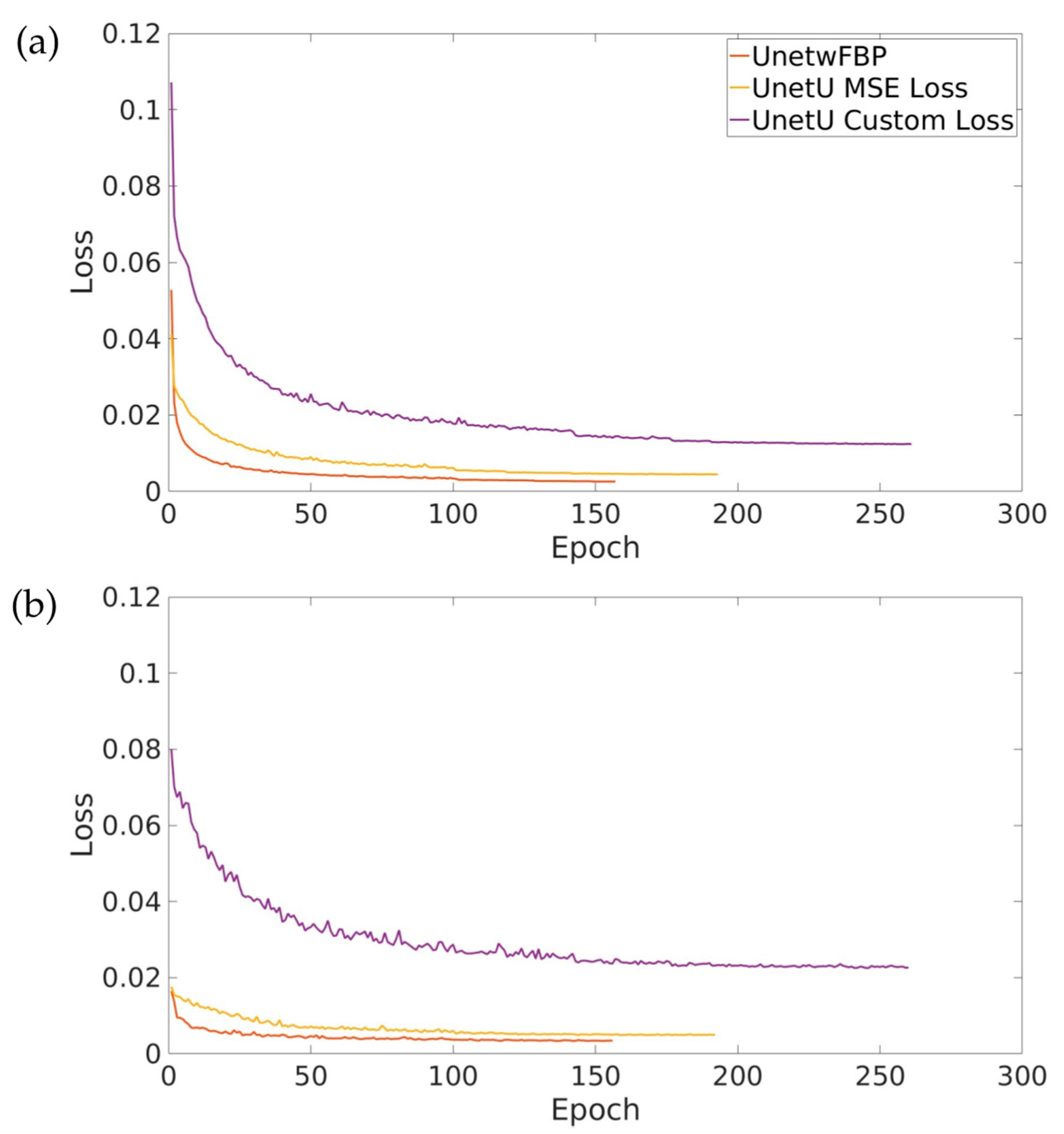
3.1. Loss Curves
3.2. Computation Time
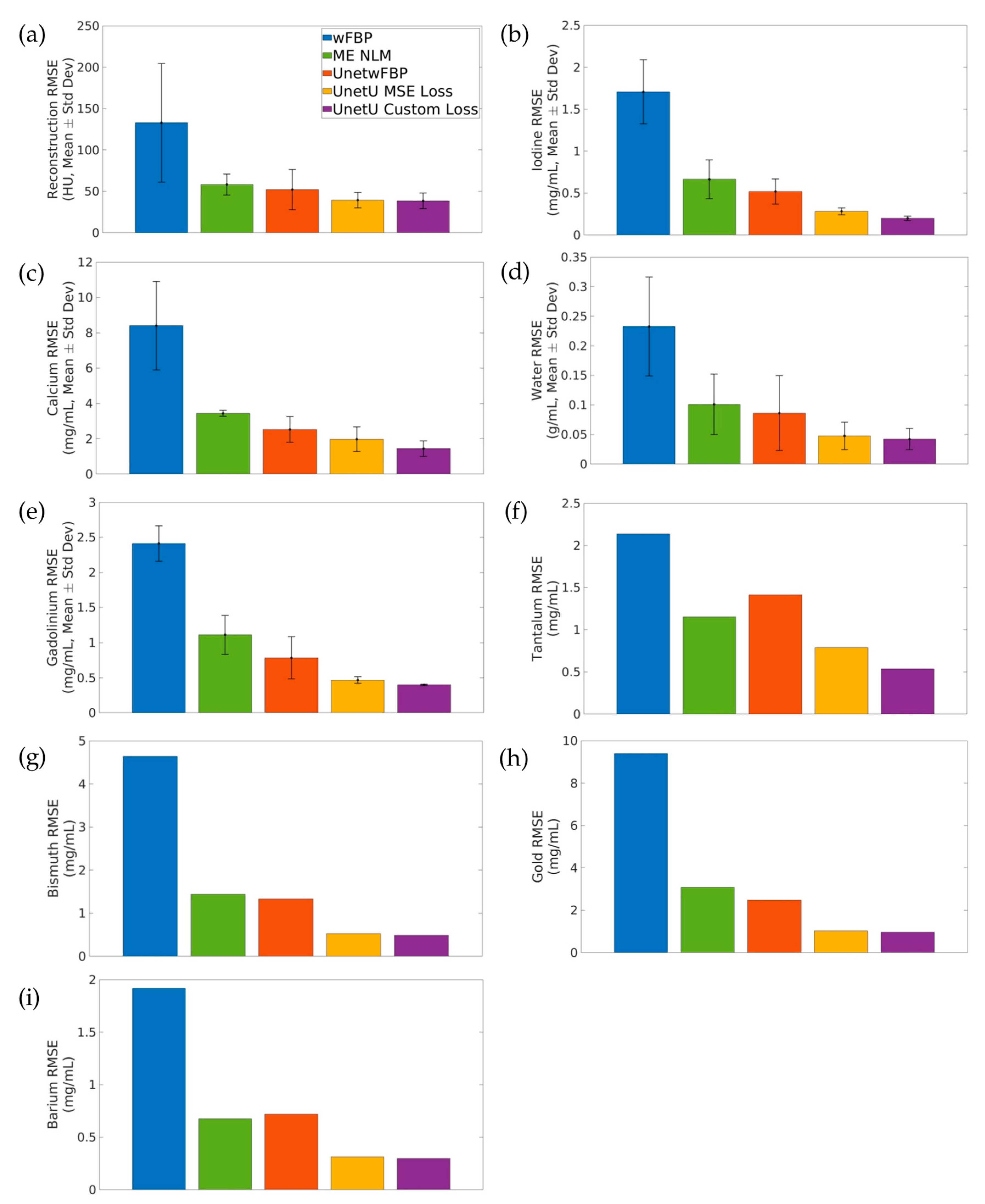
3.3. Quantitative Analyses
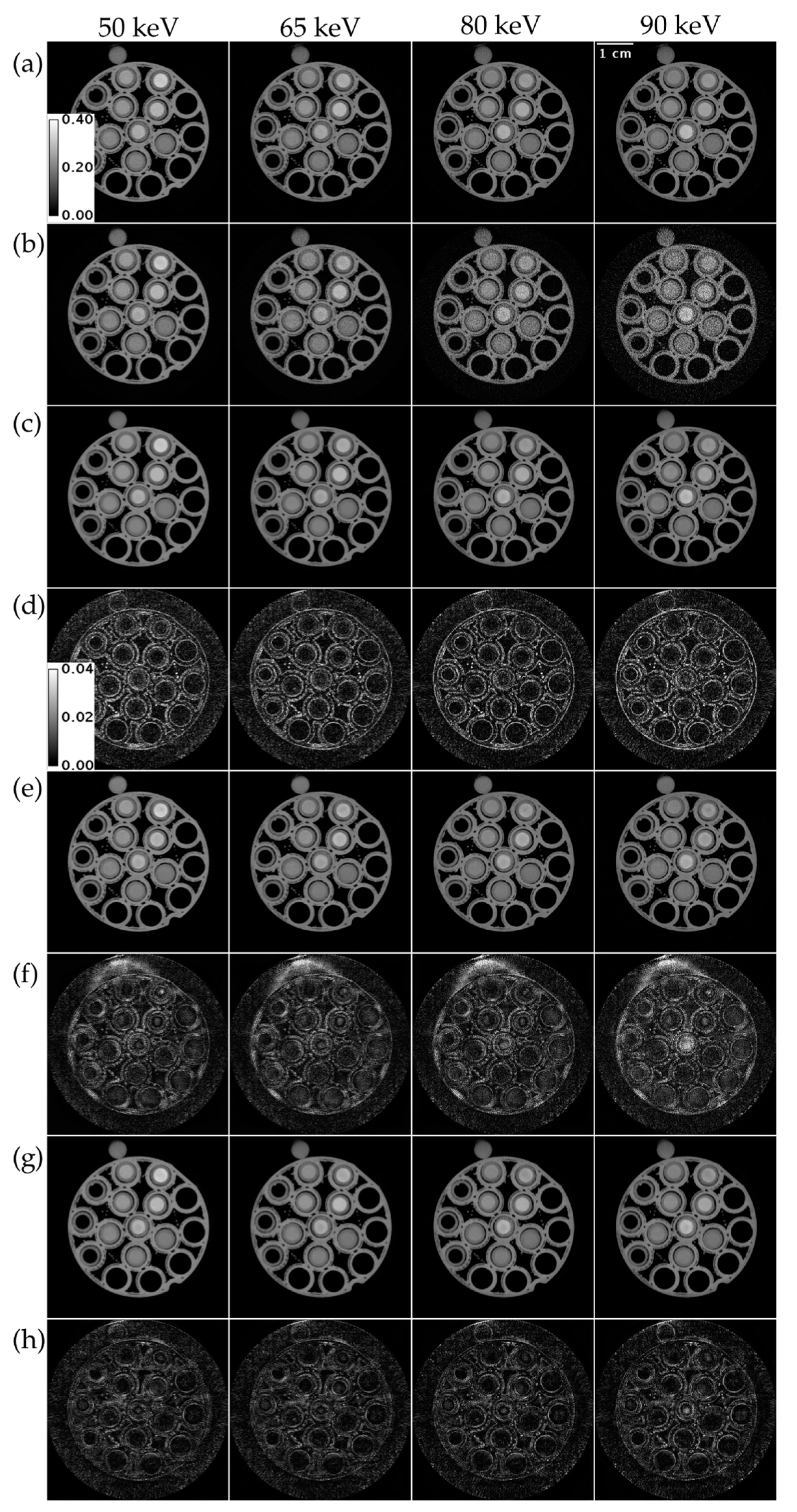
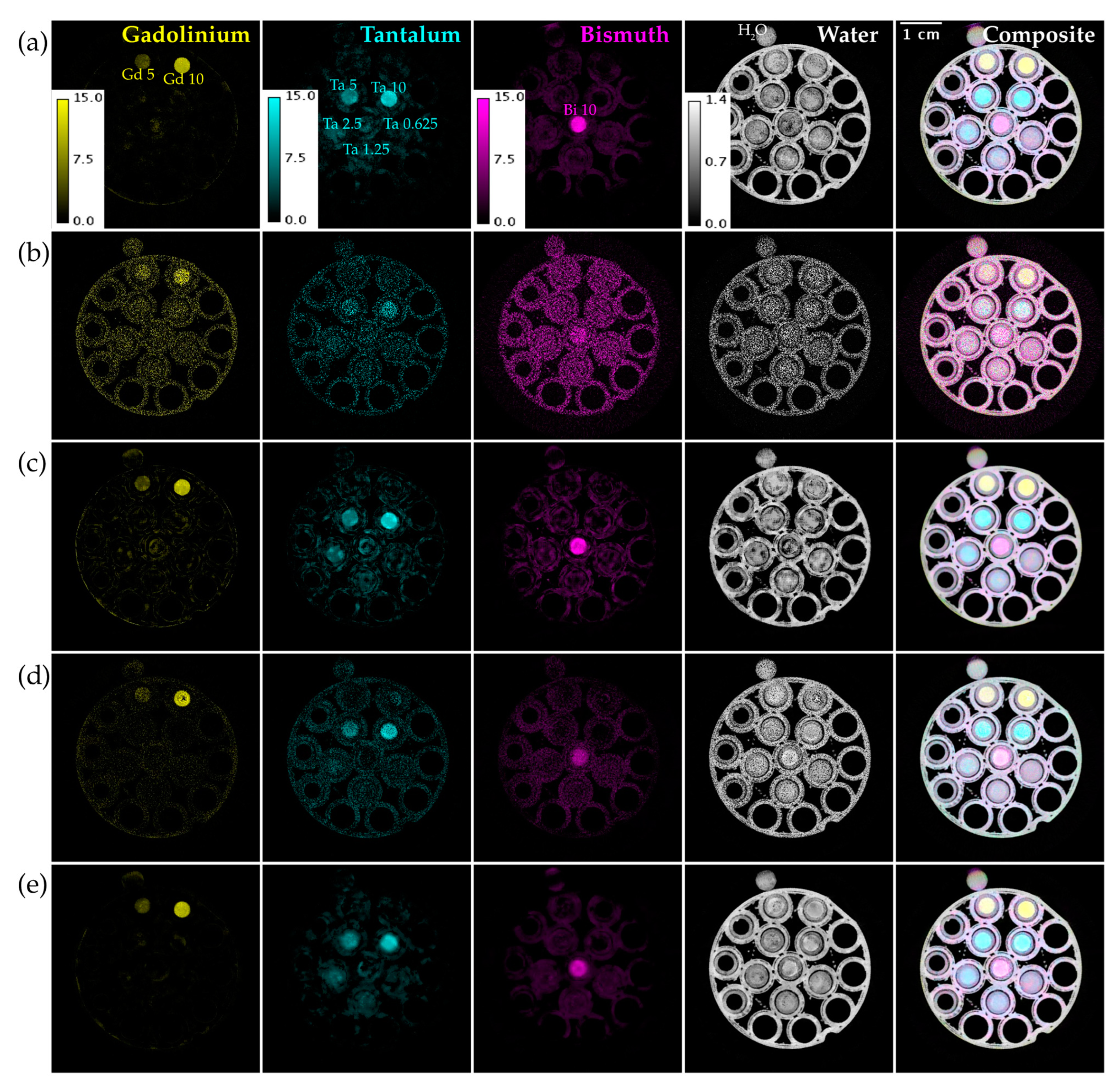
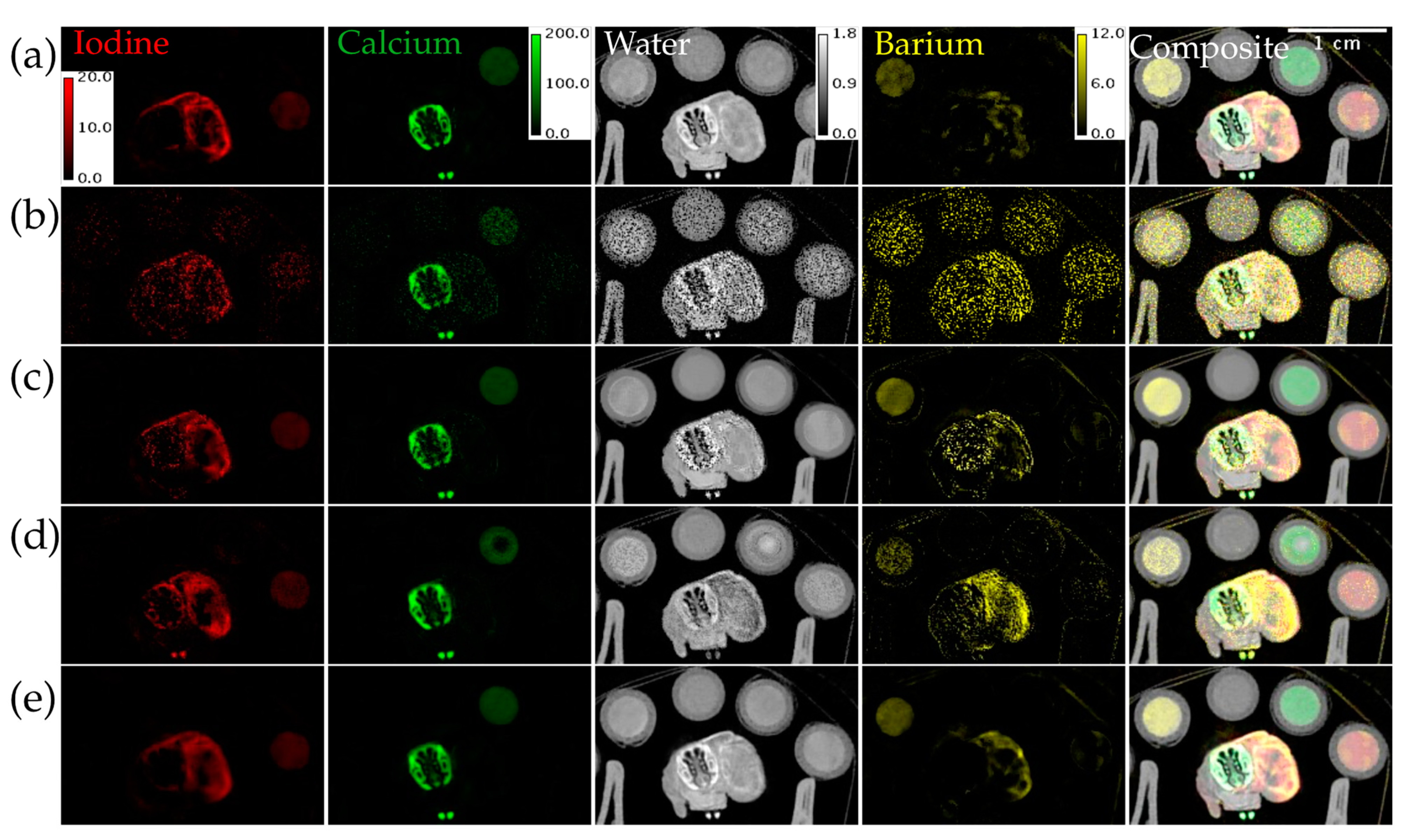
3.4. Vials Phantom
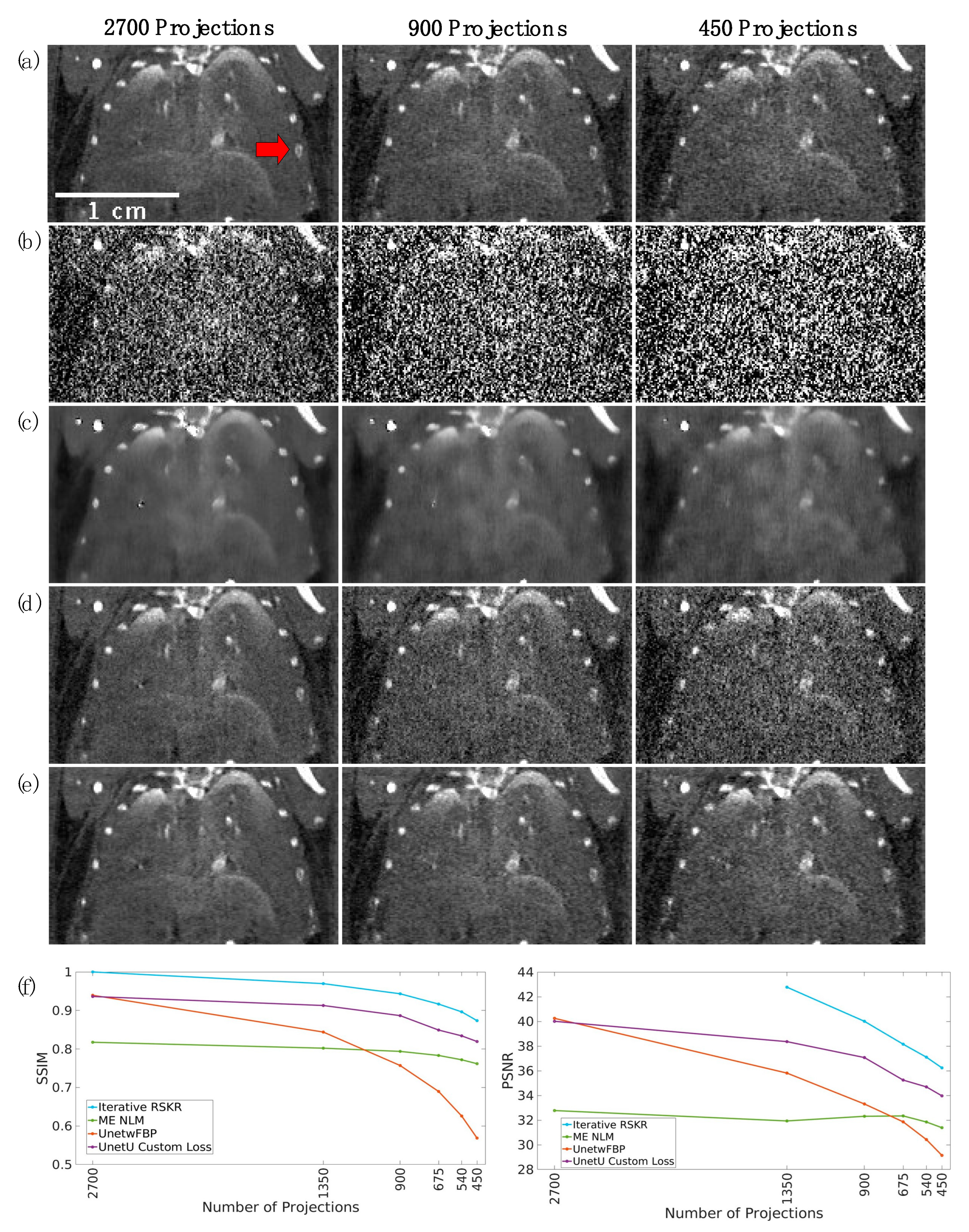
3.5. In Vivo Mouse Scan
3.6. Performance at Different Dose Levels
4. Discussion
5. Conclusions
Author Contributions
Funding
Institutional Review Board Statement
Informed Consent Statement
Data Availability Statement
Acknowledgments
Conflicts of Interest
References
- Taguchi, K.; Iwanczyk, J.S. Vision 20/20: Single photon counting X-ray detectors in medical imaging. Med. Phys. 2013, 40, 100901. [Google Scholar] [CrossRef] [Green Version]
- Leng, S.; Bruesewitz, M.; Tao, S.; Rajendran, K.; Halaweish, A.F.; Campeau, N.; Fletcher, J.G.; McCollough, C.H. Photon-counting Detector CT: System Design and Clinical Applications of an Emerging Technology. RadioGraphics 2019, 39, 609–912. [Google Scholar] [CrossRef] [PubMed]
- Allphin, A.J.; Clark, D.P.; Thuering, T.; Bhandari, P.; Ghaghada, K.B.; Badea, C.T. Micro-CT imaging of multiple K-edge elements using GaAs and CdTe photon counting detectors. Phys. Med. Biol. 2023, 68, 085023. [Google Scholar] [CrossRef] [PubMed]
- Li, Z.; Yu, L.; Trzasko, J.D.; Lake, D.S.; Blezek, D.J.; Fletcher, J.G.; McCollough, C.H.; Manduca, A. Adaptive nonlocal means filtering based on local noise level for CT denoising. Med. Phys. 2014, 41, 011908. [Google Scholar] [CrossRef]
- Li, Z.; Leng, S.; Yu, L.; Manduca, A.; McCollough, C.H. An effective noise reduction method for multi-energy CT images that exploit spatio-spectral features. Med. Phys. 2017, 44, 1610–1623. [Google Scholar] [CrossRef] [PubMed] [Green Version]
- Mechlem, K.; Ehn, S.; Sellerer, T.; Braig, E.; Munzel, D.; Pfeiffer, F.; Noel, P.B. Joint Statistical Iterative Material Image Reconstruction for Spectral Computed Tomography Using a Semi-Empirical Forward Model. IEEE Trans. Med. Imaging 2018, 37, 68–80. [Google Scholar] [CrossRef]
- Niu, S.; Zhang, Y.; Zhong, Y.; Liu, G.; Lu, S.; Zhang, X.; Hu, S.; Wang, T.; Yu, G.; Wang, J. Iterative reconstruction for photon-counting CT using prior image constrained total generalized variation. Comput. Biol. Med. 2018, 103, 167–182. [Google Scholar] [CrossRef] [PubMed]
- Yu, Z.; Leng, S.; Li, Z.; McCollough, C.H. Spectral prior image constrained compressed sensing (spectral PICCS) for photon-counting computed tomography. Phys. Med. Biol. 2016, 61, 6707–6732. [Google Scholar] [CrossRef] [Green Version]
- Baffour, F.I.; Huber, N.R.; Ferrero, A.; Rajendran, K.; Glazebrook, K.N.; Larson, N.B.; Kumar, S.; Cook, J.M.; Leng, S.; Shanblatt, E.R.; et al. Photon-counting Detector CT with Deep Learning Noise Reduction to Detect Multiple Myeloma. Radiology 2023, 306, 229–236. [Google Scholar] [CrossRef]
- Clark, D.P.; Badea, C.T. Hybrid spectral CT reconstruction. PLoS ONE 2017, 12, e0180324. [Google Scholar] [CrossRef] [Green Version]
- Jin, K.H.; McCann, M.T.; Froustey, E.; Unser, M. Deep Convolutional Neural Network for Inverse Problems in Imaging. IEEE Trans. Image Process. 2017, 26, 4509–4522. [Google Scholar] [CrossRef] [PubMed] [Green Version]
- Wang, S.; Yang, Y.; Yin, Z.; Wang, A. Noise2Noise for denoising photon counting CT images: Generating training data from existing scans. Proceedings of SPIE Medical Imaging 2023: Physics of Medical Imaging, San Diego, CA, USA.
- Chen, H.; Zhang, Y.; Kalra, M.K.; Lin, F.; Chen, Y.; Liao, P.; Zhou, J.; Wang, G. Low-Dose CT With a Residual Encoder-Decoder Convolutional Neural Network. IEEE Trans. Med. Imaging 2017, 36, 2524–2535. [Google Scholar] [CrossRef]
- Yang, Q.; Yan, P.; Zhang, Y.; Yu, H.; Shi, Y.; Mou, X.; Kalra, M.K.; Zhang, Y.; Sun, L.; Wang, G. Low-Dose CT Image Denoising Using a Generative Adversarial Network With Wasserstein Distance and Perceptual Loss. IEEE Trans. Med. Imaging 2018, 37, 1348–1357. [Google Scholar] [CrossRef]
- Wang, D.; Fan, F.; Wu, Z.; Liu, R.; Wang, F.; Yu, H. CTformer: Convolution-free Token2Token dilated vision transformer for low-dose CT denoising. Phys. Med. Biol. 2023, 68, 065012. [Google Scholar] [CrossRef] [PubMed]
- Huber, N.R.; Ferrero, A.; Rajendran, K.; Baffour, F.; Glazebrook, K.N.; Diehn, F.E.; Inoue, A.; Fletcher, J.G.; Yu, L.; Leng, S.; et al. Dedicated convolutional neural network for noise reduction in ultra-high-resolution photon-counting detector computed tomography. Phys. Med. Biol. 2022, 67, 175014. [Google Scholar] [CrossRef] [PubMed]
- Heinrich, M.P.; Stille, M.; Buzug, T.M. Residual U-Net Convolutional Neural Network Architecture for Low-Dose CT Denoising. Curr. Dir. Biomed. Eng. 2018, 4, 297–300. [Google Scholar] [CrossRef]
- Abascal, J.F.P.J.; Bussod, S.; Ducros, N.; Si-Mohamed, S.; Douek, P.; Chappard, C.; Peyrin, F. A residual U-Net network with image prior for 3D image denoising. In Proceedings of the 2020 28th European Signal Processing Conference (EUSIPCO), Amsterdam, The Netherlands, 18–21 January 2021; pp. 1264–1268. [Google Scholar]
- Yuan, N.; Zhou, J.; Qi, J. Half2Half: Deep neural network based CT image denoising without independent reference data. Phys. Med. Biol. 2020, 65, 215020. [Google Scholar] [CrossRef]
- Wu, W.; Hu, D.; Niu, C.; Vanden Broeke, L.; Butler, A.P.H.; Cao, P.; Atlas, J.; Chernoglazov, A.; Vardhanabhuti, V.; Wang, G. Deep learning based spectral CT imaging. Neural Netw. 2021, 144, 342–358. [Google Scholar] [CrossRef]
- Komatsu, R.; Gonsalves, T. Comparing U-Net Based Models for Denoising Color Images. AI 2020, 1, 465–486. [Google Scholar] [CrossRef]
- Holbrook, M.D.; Clark, D.P.; Badea, C.T. Dual source hybrid spectral micro-CT using an energy-integrating and a photon-counting detector. Phys. Med. Biol. 2020, 65, 205012. [Google Scholar] [CrossRef]
- Stierstorfer, K.; Rauscher, A.; Boese, J.; Bruder, H.; Schaller, S.; Flohr, T. Weighted FBP—A simple approximate 3D FBP algorithm for multislice spiral CT with good dose usage for arbitrary pitch. Phys. Med. Biol. 2004, 49, 2209–2218. [Google Scholar] [CrossRef] [PubMed]
- Gao, H.; Yu, H.; Osher, S.; Wang, G. Multi-energy CT based on a prior rank, intensity and sparsity model (PRISM). Inverse Probl. 2011, 27, 115012. [Google Scholar] [CrossRef] [PubMed] [Green Version]
- Alvarez, R.E.; Macovski, A. Energy-selective reconstructions in X-ray computerised tomography. Phys. Med. Biol. 1976, 21, 733–744. [Google Scholar] [CrossRef]
- Ronneberger, O.; Fischer, P.; Brox, T. U-Net: Convolutional Networks for Biomedical Image Segmentation. In Proceedings of the Medical Image Computing and Computer-Assisted Intervention–MICCAI 2015, 18th International Conference, Munich, Germany, 5–9 October 2015; Springer: Cham, Switzerland, 2015; pp. 234–241. [Google Scholar]
- Paszke, A.; Gross, S.; Massa, F.; Lerer, A.; Bradbury, J.; Chanan, G.; Killeen, T.; Lin, Z.M.; Gimelshein, N.; Antiga, L.; et al. PyTorch: An Imperative Style, High-Performance Deep Learning Library. Adv. Neural Inf. Process. Syst. 2019, 32, 721. [Google Scholar]
- Donoho, D.L.; Johnstone, I.M. Adapting to Unknown Smoothness via Wavelet Shrinkage. J. Am. Stat. Assoc. 1995, 90, 1200–1224. [Google Scholar] [CrossRef]
- Kingma, D.P.; Ba, J.L. Adam: A Method for Stochastic Optimization. In Proceedings of the 3rd International Conference on Learning Representations, ICLR 2015, San Diego, CA, USA, 7–9 May 2015. [Google Scholar]
- Nadkarni, R.; Allphin, A.; Clark, D.P.; Badea, C.T. Material decomposition from photon-counting CT using a convolutional neural network and energy-integrating CT training labels. Phys. Med. Biol. 2022, 67, 155003. [Google Scholar] [CrossRef] [PubMed]


| PCD Thresholds (keV) | Training Sets | Validation Sets | Test Sets | Contrast Materials | kVp | mA | Dose (mGy) | Types of Samples Scanned |
|---|---|---|---|---|---|---|---|---|
| 25, 34, 50, 60 | 3 | 0 | 1 | I, Gd | 80 | 4 | 36 | in vivo, ex vivo |
| 25, 34, 50, 80 | 2 | 1 | 1 | I, Au | 125 | 2.5 | 38 | ex vivo |
| 25, 28, 34, 40 | 2 | 0 | 1 | I | 80 | 4 | 36 | ex vivo, phantom |
| 50, 65, 80, 90 | 2 | 0 | 1 | Gd, Ta, Bi | 125 | 2.5 | 38 | ex vivo, phantom |
| 28, 34, 39, 45 | 0 | 0 | 1 | I, Ba | 80 | 4 | 36 | in vivo |
Disclaimer/Publisher’s Note: The statements, opinions and data contained in all publications are solely those of the individual author(s) and contributor(s) and not of MDPI and/or the editor(s). MDPI and/or the editor(s) disclaim responsibility for any injury to people or property resulting from any ideas, methods, instructions or products referred to in the content. |
© 2023 by the authors. Licensee MDPI, Basel, Switzerland. This article is an open access article distributed under the terms and conditions of the Creative Commons Attribution (CC BY) license (https://creativecommons.org/licenses/by/4.0/).
Share and Cite
Nadkarni, R.; Clark, D.P.; Allphin, A.J.; Badea, C.T. A Deep Learning Approach for Rapid and Generalizable Denoising of Photon-Counting Micro-CT Images. Tomography 2023, 9, 1286-1302. https://0-doi-org.brum.beds.ac.uk/10.3390/tomography9040102
Nadkarni R, Clark DP, Allphin AJ, Badea CT. A Deep Learning Approach for Rapid and Generalizable Denoising of Photon-Counting Micro-CT Images. Tomography. 2023; 9(4):1286-1302. https://0-doi-org.brum.beds.ac.uk/10.3390/tomography9040102
Chicago/Turabian StyleNadkarni, Rohan, Darin P. Clark, Alex J. Allphin, and Cristian T. Badea. 2023. "A Deep Learning Approach for Rapid and Generalizable Denoising of Photon-Counting Micro-CT Images" Tomography 9, no. 4: 1286-1302. https://0-doi-org.brum.beds.ac.uk/10.3390/tomography9040102