Toward an Automated-Algebra Framework for High Orders in the Virial Expansion of Quantum Matter

Abstract

The virial expansion provides a non-perturbative view into the thermodynamics of quantum many-body systems in dilute regimes. While powerful, the expansion is challenging as calculating its coefficients at each order n requires analyzing (if not solving) the quantum n-body problem. In this work, we present a comprehensive review of automated algebra methods, which we developed to calculate high-order virial coefficients. The methods are computational but non-stochastic, thus avoiding statistical effects; they are also for the most part analytic, not numerical, and amenable to massively parallel computer architectures. We show formalism and results for coefficients characterizing the thermodynamics (pressure, density, energy, static susceptibilities) of homogeneous and harmonically trapped systems and explain how to generalize them to other observables such as the momentum distribution, Tan contact, and the structure factor.

1. Introduction

Quantum many-body systems are notoriously difficult to compute. Whenever interactions play an important role, in atomic, condensed matter, or nuclear physics, most analytic approaches (if not all) are unable to give quantitatively reliable results and numerical methods often face challenges of their own as well, such as the infamous sign problem (notwithstanding remarkable progress over the last few years) [1].

The virial expansion (VE) (see, e.g., Reference [2] for an introduction to both the classical and quantum cases and Reference [3] for a comprehensive review) aims to tackle the finite-temperature quantum many-body problem by breaking it down into contributions from subspaces of the full Fock space corresponding to a fixed (and small) particle number. In this sense, the VE is effectively an expansion around a dilute limit in which the interparticle distance is much larger than every other scale in the system, in particular the thermal wavelength ${\lambda }_T=\sqrt{2\pi \beta }$, where $\beta =1/T$ is the inverse temperature and we have used units such that $\hslash =k_B=m=1$. With this being a high-temperature regime (as ${\lambda }_T$ is in the above sense small), one might expect that interaction effects would play a quantitatively minor role; this, however, is not necessarily the case, as we will see. Another misconception is that quantum effects play a small role in such a regime, which is also not generally true. Both interaction and quantum effects are central in the calculation of the virial expansion and leave a clear imprint in the expansion coefficients. It is for that reason that such calculations are challenging and that specialized techniques are required to carry them out, as we explain in this review. However, we are getting ahead of ourselves; let us start from the beginning.

The origin of the VE is the classical cluster expansion of Mayer et al., developed in the 1930s [4], in which the classical grand-canonical partition function $\mathcal{Z}$ of a three-dimensional gas is expanded in powers of the fugacity $z=exp\left(\beta \mu \right)$, where $\mu$ is the chemical potential, namely

$$\mathcal{Z}=\sum _{N=0}^{\infty }{\left(\frac{z}{{\lambda }_T^3}\right)}^N\frac{Q_N}{N!},$$

(1)

where

$$Q_N=\int \prod _{i=1}^{N}d{\mathbf{r}}_i{e}^{-\frac{\beta }{2}{\sum }_{i\ne j}{V}_{ij}},$$

(2)

is the classical canonical partition function and $V_{ij}$ is the pairwise interaction potential between particle i and particle j.

An expansion of both the pressure P and the number density n in powers of z is thus obtained, namely

$$\begin{array}{ccc}\hfill \beta P& =& \frac{1}{{\lambda }_T^3}\sum _{k=1}^{\infty }{b}_k{z}^k,\hfill \end{array}$$

(3)

$$\begin{array}{ccc}\hfill n& =& \frac{1}{{\lambda }_T^3}\sum _{k=1}^{\infty }k{b}_k{z}^k,\hfill \end{array}$$

(4)

where the $b_k$, originally called ‘cluster coefficients’, typically depend on temperature and the specific form of $V_{ij}$. Substituting the density expansion into the pressure expansion, order by order in z, one obtains the old virial expansion of the imperfect gas equation of state in powers of the density, i.e.,

$$P=n{k}_{B}T\sum _{k=1}^{\infty }{a}_k{x}^{k-1},$$

(5)

where $x=n{\lambda }_T^3$ and the $a_k$ are in older literature called ‘virial coefficients’ (more recently, that nomenclature has been used for the $b_k$ coefficients instead). Calculating the $a_k$ requires knowing all the b coefficients up to order k, which in turn requires calculating the canonical partition functions of up to k particles, as we will show in more detail below. The original work of Mayer et al. proposed a diagrammatic technique for calculating the classical case, which is naturally simpler than its quantum counterpart simply because of the well-known fact that kinetic and potential energies are commuting numbers in the classical case and non-commuting operators in the quantum case. The quantum virial expansion was first explored by Kahn and Uhlenbeck [5] and further developed by Lee and Yang [6,7,8,9,10]. As we review below, the calculation of $b_k$ for the quantum case is so challenging in practice that efforts to calculate the third-order coefficient and beyond were not successful until the 21st century, when computers became powerful enough to apply exact diagonalization techniques. From this point on, we focus entirely on the VE in the context of quantum systems.

Historically, applications of the VE have followed the above paradigm and thus centered on equations of state. However, since the VE is an expansion of the grand-canonical partition function, it is possible to apply it to any physical quantity. We will show techniques to calculate the VE for applications to pressure and density but also to the Tan contact [11,12,13] (relevant for systems with short-range interactions), the momentum distribution, and response functions such as the compressibility and the structure factor.

The recent developments of automated algebra, led by our group [14,15,16,17,18,19,20,21], have enabled the precise calculation of high-order coefficients (meaning beyond the third order, which can currently be addressed numerically). With such orders in hand, it becomes practical and meaningful to implement resummation techniques which, uncertainties notwithstanding, have been shown to substantially extend the domain of applicability of the virial expansion [18,19].

The remainder of this work is organized as follows. We begin in Section 2 by reviewing the formal elements of the virial expansion of the grand thermodynamic potential, as that is the simplest case, which also allows us to establish the basic identities and notation. In Section 3, we provide a brief review of conventional calculation methods for the virial coefficients. In Section 4, we present our method by example using a homogeneous system of Fermion gases with attractive interaction changing from the non-interacting limit to the unitary limit. Encouraged by the agreements with and improvements over existing results, we further generalize the method to other systems in Section 5, including harmonically trapped systems in Section 5.1, neutron matter in Section 5.2, and the unitary Bose gas in Section 5.3. Finally, Section 6.2 demonstrates the applications to more complicated observables. Namely, one-body operators such as density or momentum distributions are discussed in Section 6.2, and two-body operators, which are of interest to quantities such as the structure factor or viscosity, are shown in Section 6.3.

2. Basic Formalism

As mentioned above, the VE is an expansion in powers of the fugacity z

$$z=e^{\beta \mu },$$

(6)

where $\beta$ is the inverse temperature and $\mu$ is the chemical potential. In the presence of spin or other internal degrees of freedom, there will naturally be a fugacity attached to each (conserved) particle number. In this section, we present the formalism for a single flavor for simplicity, but in upcoming sections we will generalize it to spin-$1/2$ fermions.

The thermodynamics is encoded in the grand-canonical partition function, which for a quantum system is given by

$$\mathcal{Z}=\mathrm{Tr}\left[e^{-\beta (\widehat{H}-\mu \widehat{N})}\right],$$

(7)

where $\widehat{H}$ is the Hamiltonian, $\widehat{N}$ is the particle number operator, and $\mu$ is the chemical potential. Expanding $\mathcal{Z}$ in powers of the fugacity, we obtain

$$\mathcal{Z}=\sum _{N=0}^{\infty }{z}^N{Q}_N,$$

(8)

where

$$Q_N={\mathrm{tr}}_N^{}\left[e^{-\beta \widehat{H}}\right],$$

(9)

is the canonical N-particle partition function.

Then, the grand thermodynamic potential is expanded in powers of z using the above expressions to obtain the conventional expression

$$-\beta \Omega =\beta PV=ln\mathcal{Z}=Q_1\sum _{k=1}^{\infty }{z}^k{b}_k,$$

(10)

where $b_k$ is the k-th order virial coefficient, which is an intensive, dimensionless quantity. Through Equations (8) and (10), the $b_k$ are related to the canonical partition functions; for example, the first few $b_k$ are

$$\begin{array}{cc}\hfill b_1=& 1,\hfill \\ \hfill b_2=& \frac{Q_2}{Q_1}-\frac{Q_1}{2!},\hfill \\ \hfill b_3=& \frac{Q_3}{Q_1}-b_2{Q}_1-\frac{Q_1^2}{3!},\hfill \\ \hfill b_4=& \frac{Q_4}{Q_1}-\left(b_3+\frac{b_2^2}{2}\right)Q_1-b_2\frac{Q_1^2}{2!}-\frac{Q_1^3}{4!}.\hfill \end{array}$$

(11)

For a system of non-interacting, non-relativistic fermions in d dimensions, the virial coefficients are

$$b_k^{\left(0\right)}={(-1)}^{k+1}{k}^{-(d+2)/2},$$

(12)

whereas for bosons the result is simply $k^{-(d+2)/2}$. In the presence of interactions, one usually expands the ratio of $\mathcal{Z}$ to its non-interacting counterpart ${\mathcal{Z}}_0$, to obtain

$$-\beta \Delta \Omega =ln(\mathcal{Z}/{\mathcal{Z}}_0)=Q_1\sum _{k=1}^{\infty }{z}^k\Delta b_k,$$

(13)

where $\Delta b_k=b_k-b_k^{\left(0\right)}$ captures the interaction effects and is the quantity most often reported. In practice, the $\Delta b_k$ coefficients are determined by the interaction-induced change in $Q_j$ for $1<j\le k$, and therein lies the difficulty: those $Q_j$ must be determined with enough accuracy to cancel out all the volume dependence (which contains terms that scale with power up to j) and obtain a volume-independent $\Delta b_k$. As we will see below, some methods focus on extracting $\Delta b_k$ directly from grand-canonical quantities (typically the density), where the volume cancellations have already happened, while others such as ours (and similarly exact diagonalization) propose to calculate the interaction effects on $Q_j$ and use those to calculate $\Delta b_k$.

The above is the VE as applied to the pressure; from it, the expansion for the density is easily derived. As mentioned above, the VE can, in fact, be applied to any observable such as Tan contact, the momentum distribution, and the structure factor (see Section 6.3). We will return to those in a later section.

3. Calculation Methods for the Virial Expansion

3.1. Second Order

In addition to the trivial one-body contribution, fully captured by $Q_1$ and factored out of the expansion, the leading contribution accounting for interaction effects appears at second order, i.e., the two-particle subspace. The interaction effects on the two-particle spectrum are captured by the scattering properties (binding energies and phase shifts), and in those terms, the second-order virial coefficient $b_2$ was first calculated analytically by Beth and Uhlenbeck in the 1930s [22,23]. Specifically, their result relates the interaction change $\Delta b_2$ to the two-body scattering phase shift $\delta \left(E\right)$ such that, for a spin-1/2 Fermi gas in three spatial dimensions (3D),

$$\Delta b_2=\sqrt{2}\sum _i{e}^{-\beta E_B^i}+\sqrt{2}\sum _l\frac{2l+1}{\pi }{\int }_0^{\infty }dp\frac{d{\delta }_l}{dp}{e}^{-\frac{{\lambda }_T^2{p}^2}{2\pi }}$$

(14)

where the first summation is overall bound states and the second summation is overall partial waves.

One may take the above expression in different dimensions and relate it to the parameters of the corresponding effective range expansion (i.e., scattering length, effective range, etc.) and obtain, for a zero-range interaction (see, e.g., [24,25] for results in 1D, [26,27] for 2D, and [28] for 3D):

$$\begin{array}{cc}\hfill \Delta b_2^{1\mathrm{D}}& =-\frac{1}{2\sqrt{2}}+\frac{e^{{\lambda }_1^2/4}}{2\sqrt{2}}\left[1+\mathrm{erf}({\lambda }_1/2)\right],\hfill \\ \hfill \Delta b_2^{2\mathrm{D}}& =e^{{\lambda }_2^2}-2{\int }_0^{\infty }\frac{dp}{p}\frac{2e^{-{\lambda }_2^2{p}^2}}{{\pi }^2+4{ln}^2\left(p^2\right)},\hfill \\ \hfill \Delta b_2^{3\mathrm{D}}& =\frac{e^{{\lambda }_3^2}}{\sqrt{2}}\left[1+\mathrm{erf}\left({\lambda }_3\right)\right],\hfill \end{array}$$

(15)

where ${\lambda }_d$ is the physical coupling strength in d dimensions, defined as

$$\begin{array}{cc}\hfill {\lambda }_1& =2\frac{\sqrt{\beta }}{a_0},\hfill \\ \hfill {\lambda }_2& =\sqrt{\beta E_B},\hfill \\ \hfill {\lambda }_3& =\frac{\sqrt{\beta }}{a_0},\hfill \end{array}$$

(16)

where $a_0$ is the s-wave scattering length and $E_B$ is the binding energy of the single two-body bound state of the 2D case.

While the above results are sufficient for simple systems such as dilute gases of ultracold atoms, where the interaction can be modeled very precisely as being purely zero-range s-wave, a deeper analysis is needed to account for the complexities of nuclear systems (such as neutron and nuclear matter). References [29,30] presented such an extension of the 3D case to the richer scattering properties found in nuclear physics. There, one must account for not only a finite range but also angular momentum channels beyond the simplest case of pure s-wave. For pure neutron matter, References [29,30] integrate by parts to rewrite the Beth–Uhlenbeck result as

$$\Delta b_2=\frac{1}{2^{1/2}\pi T}{\int }_0^{\infty }dE{e}^{-\beta E/2}{\delta }_{\mathrm{neutrons}}^{\mathrm{tot}}\left(E\right),$$

(17)

where ${\delta }_{\mathrm{neutrons}}^{\mathrm{tot}}\left(E\right)$ is the sum of all the scattering phase shifts at laboratory energy E, whose contributions from different angular momentum channels enter as

$${\delta }_{\mathrm{neutrons}}^{\mathrm{tot}}\left(E\right)=\sum _{S,L,J}(2J+1){\delta }_{{}^{2S+1}{L}_J}\left(E\right),$$

(18)

where the partial wave terms ${\delta }_{{}^{2S+1}{L}_J}\left(E\right)$ are obtained from partial wave analyses of experimental data such as Nijmegen’s [31].

For nuclear matter, on the other hand, one must account for the deuteron bound state, such that

$$\Delta b_2=\frac{3}{2^{1/2}}\left(e^{E_d/T}-1\right)+\frac{1}{2^{3/2}\pi T}{\int }_0^{\infty }dE{e}^{-\beta E/2}{\delta }_{\mathrm{nuc}}^{\mathrm{tot}}\left(E\right),$$

(19)

where $E_d$ is the binding energy of the deuteron and the $-1$ term comes from partial integration when accounting for the phase shift at zero energy being $\pi$ times the number of bound states (see also Reference [32]). The work of References [29,30] also analyzed the contributions due to pure alpha-particle scattering and nucleon-alpha scattering, thus obtaining all possible contributions to the second-order virial expansion for nuclear matter composed of neutrons, protons, and alpha particles.

3.2. Third Order and Beyond

The complexity of the quantum many-body problem for three particles and beyond forces one to switch to a combination of analytic and numerical approaches to calculate virial coefficients beyond the second order. In cases of great interest such as spin-$1/2$ fermions, one has to further break up the problem into the subspaces of fixed particle number; for example, calculating $\Delta b_4$ requires solving the problem of $3+1$ particles (i.e., 3 spin up and 1 spin down, and vice versa) as well as $2+2$ particles. The number of such subspaces naturally proliferates with higher total particle number, and furthermore each subspace may present its own difficulties.

To calculate $\Delta b_3$ there is only one distinct subspace that matters, namely $2+1$ particles (assuming that both particles have the same mass), and impressive exact analytic progress was made by several authors, notably the work of Leyronas [33], Kaplan and Sun [34], and Castin and colleagues [35,36,37,38], as well as the large effective range expansion of Ngampruetikorn et al. [39] (see also the early work of Reference [40] focusing on the unitary limit). There are other works focusing on this area, but they are omitted from this review as their methods or formalism are beyond our scope. Readers may be interested in References [41,42], which discuss related work.

Leyronas organizes the calculation of $\Delta b_k$ around the VE of the density equation of state, itself expressed as an integral over all momenta of the equal-time single-particle Green’s function in momentum space (i.e., the momentum distribution). Diagrams of various types are then identified at each order in z (up to order $z^3$), where contributions from the 2- and 3-body T matrix appear (the latter describing the atom-dimer scattering). The resulting time integrals are converted into energy integrals, which are then evaluated analytically where possible and otherwise numerically. The resulting approach is thus for the most part analytic and in principle exact and is in remarkable agreement in the unitary limit with prior purely numerical results for $b_3$ [43].

Other diagrammatic approaches also made interesting contributions. The work of Kaplan and Sun [34], which preceded Leyronas, starts from the density equation-of-state written as a momentum integral over the single-particle Green’s function (as Leyronas does), but rather than carrying out the Matsubara sum from the outset, it uses a Poisson summation to express the propagator directly as a power series in z. The latter is then interpreted as a sum over the winding number of worldlines around the compact imaginary time direction. The diagrams associated with each term in that expansion are referred to as ‘chronographs’. Adding the contributions from such chronographs and accounting for systematic effects by extrapolation, very good agreement with prior numerical results [43] for $b_3$ was obtained in the unitary limit.

Ngampruetikorn et al. [39] used an expansion around large effective range $R^{*}$ (compared to the thermal wavelength ${\lambda }_T$), which allows them to examine up to the four-particle subspace diagrammatically, thus obtaining numerical estimates for up to $\Delta b_4$. They focused on the unitary Fermi gas by interpolating between $R^{*}\gg {\lambda }_T$ and ${\lambda }_T/\left|a\right|\gg 1$, where a is the scattering length, and applied their method to the pressure, density, entropy, and spectral functions. Their interpolation results for $\Delta b_3$ and $\Delta b_4$ at unitarity agree with those obtained by other groups, including those presented here. In Reference [44], Ngampruetikorn et al. also studied the pairing correlations of the 2D Fermi gas up to third order in the virial expansion, additionally obtaining Tan contact (we return to the expansion of this and other quantities below).

In Reference [45], Werner and Castin analyzed the (2 + 1)-body problem of harmonically trapped spin-$1/2$ fermions at unitarity, obtaining their exact spectrum and eigenstates. Generalizing that work to the problem of 3 + 1 and 2 + 2 particles, Endo and Castin [36,37] (see also [38]) calculated the value of $\Delta b_4$ as a function of the trapping frequency $\beta \omega$. As we will show in Section 5.1, our non-perturbative determination turned out to be in remarkable agreement with their result, which they considered to be only a conjecture.

On the numerical side, some of the early works used exact diagonalization in hyperspherical coordinates [35,43], whereby a large number of eigenstates can be calculated and their energies summed over to calculate canonical partition functions, thus providing access to $b_3$ (and to some extent $b_4$, and with low accuracy $b_5$) for systems of cold atoms with short-range interactions.

In an outstanding numerical feat, Yan and Blume [46,47] designed an ad hoc Monte Carlo method to tackle the calculation of $\Delta b_4$ for fermions at unitarity, resulting in the first determination of this quantity with stochastic methods. Their calculation featured a harmonic trapping potential, which induces a temperature dependence in $\Delta b_4$, which is expected to be temperature-independent in the unitary limit. (Below we will show a comparison between Yan and Blume’s results and ours, when our method is generalized to include a harmonic trap). The only important drawback of this work was the large uncertainty in the final result, induced by the increased stochastic noise as the trapping potential is removed. We will return to a discussion of this result below.

In spite of all of the above remarkable progress, it is evident that, due to the complexity of the n-particle quantum mechanical problem, a different kind of approach is needed if one is to determine high-order virial coefficients with well-controlled systematic error. In particular, stochastic methods tend to have too large uncertainties to yield the accurate estimates needed to implement resummation techniques (we return to these below). On the other hand, direct numerical methods such as exact diagonalization can be very powerful in providing detailed information (furnishing not only energies but also the associated eigenstates), but have not yet succeeded in accurately determining virial coefficients beyond the third order. One of the main objectives of this paper is to present our work in developing and applying a non-perturbative, semi-analytic, computational approach that is free of stochastic effects, beginning in the next section.

4. Homogeneous Fermi Gases with a Zero-Range Interaction

In this section, we explain our method in detail and review its application to the simplest case, namely that of Fermi gases in homogeneous space, focusing on the VE for the pressure.

4.1. Factorizing the Transfer Matrix

The cornerstone of the approach is the Suzuki–Trotter factorization of the transfer matrix (i.e., the quantum version of the Boltzmann weight). To that end, the Hamiltonian is split into kinetic and potential energy terms, i.e.,

$$\widehat{H}=\widehat{T}+\widehat{V},$$

(20)

such that the simplest symmetric Suzuki–Trotter factorization is

$$e^{-\tau \widehat{H}}=e^{-\tau \widehat{T}/2}{e}^{-\tau \widehat{V}}{e}^{-\tau \widehat{T}/2}+O\left({\tau }^3\right),$$

(21)

where $\tau$ is in principle an arbitrary parameter, but we will define it such that for some integer $N_{\tau }$, one has $\beta =\tau N_{\tau }$, i.e., $\tau$ defines the imaginary time discretization. Note that, since our interest is in taking the trace of powers of $e^{-\tau \widehat{H}}$, the same accuracy is obtained for the symmetric decomposition as for its asymmetric counterpart

$$e^{-\tau \widehat{H}}=e^{-\tau \widehat{T}}{e}^{-\tau \widehat{V}}+O\left({\tau }^2\right).$$

(22)

(Note: When calculating expectation values of operators, not mere traces, using the symmetric decomposition does make a difference.) The above factorization step is always needed in our method, regardless of whether the target system is in homogeneous space or in a trapping potential; in this section, we focus on the former, returning to the latter in a later section.

Using the above factorization, the objective is to calculate $Q_N$ for the desired particle content at progressively larger values of $N_{\tau }$. The resulting $Q_N$ is then used to calculate the $b_k$, and the limit of large $N_{\tau }$ is taken at the end by extrapolation. The latter is an extrapolation to the continuous imaginary-time limit.

The fundamental building blocks in the calculation of $Q_N$ are the matrix elements of the factorized transfer matrix. For homogeneous non-relativistic spin-1/2 fermions with a zero-range interaction, one has

$$\widehat{T}=\sum _{\sigma =\uparrow ,\downarrow }\sum _{\mathbf{p}}\frac{{\mathbf{p}}_{}^2}{2m}{\widehat{n}}_{\sigma }\left(\mathbf{p}\right),$$

(23)

where ${\widehat{n}}_{\sigma }\left(\mathbf{p}\right)$ is the number density operator for particles of spin $\sigma$ and momentum $\mathbf{p}$, and we use $m\equiv 1$ for simplicity; moreover,

$$\widehat{V}=-g{\ell }^3\sum _{\mathbf{r}}{\widehat{n}}_{\uparrow }\left(\mathbf{r}\right){\widehat{n}}_{\downarrow }\left(\mathbf{r}\right),$$

(24)

where the minus sign is for convenience for attractive interactions, ${\widehat{n}}_{\sigma }\left(\mathbf{r}\right)$ is the number density operator for particles of spin $\sigma$ at position $\mathbf{r}$, and we have regularized the problem by putting it on a spatial lattice of spacing ℓ. In practice, we renormalize this interaction by tuning it to reproduce the exact value of $b_2$, as set by the Beth–Uhlenbeck formula reviewed above.

To calculate $Q_2$, for example, the desired matrix elements are given by

$$\begin{array}{cc}\hfill {\mathcal{M}}_{11}& =\langle {\mathbf{p}}_1{\mathbf{p}}_2{e}^{-\tau \widehat{T}}{e}^{-\tau \widehat{V}}{\mathbf{q}}_1{\mathbf{q}}_2\rangle \hfill \\ \hfill & =K\left({\mathbf{p}}_1\right)K\left({\mathbf{p}}_2\right)\left[{\delta }_{{\mathbf{q}}_1,{\mathbf{p}}_1}{\delta }_{{\mathbf{q}}_2,{\mathbf{p}}_2}+C{\delta }_{{\mathbf{q}}_1+{\mathbf{q}}_2,{\mathbf{p}}_1+{\mathbf{p}}_2}\right],\hfill \end{array}$$

(25)

for the $(1+1)$-particle problem, where $K\left(\mathbf{p}\right)$ is the non-interacting, factorized Boltzmann weight

$$K\left(\mathbf{p}\right)=e^{-\tau {\mathbf{p}}^2/\left(2m\right)},$$

(26)

C is the coupling strength

$$C=e^{\tau g/{\ell }^3}-1,$$

(27)

and we use the notation

$$|\mathbf{P}\rangle =|{\mathbf{p}}_1{\mathbf{p}}_2\cdots {\mathbf{p}}_a{\mathbf{p}}_{a+1}\cdots {\mathbf{p}}_{a+b}\rangle ,$$

(28)

for the $(a+b)$-particle system, where ${\mathbf{p}}_1$ to ${\mathbf{p}}_a$ are for spin-↑ particles and ${\mathbf{p}}_{a+1}$ to ${\mathbf{p}}_{a+b}$ for spin-↓ particles.

Similarly, for the $(2+1)$-particle problem, which enters in calculating $Q_3$, one obtains

$$\begin{array}{cc}\hfill {\mathcal{M}}_{21}& =\langle {\mathbf{p}}_1{\mathbf{p}}_2{\mathbf{p}}_3{e}^{-\tau \widehat{T}}{e}^{-\tau \widehat{V}}|{\mathbf{q}}_1{\mathbf{q}}_2{\mathbf{q}}_3\rangle \hfill \\ \hfill & =K\left({\mathbf{p}}_1\right)K\left({\mathbf{p}}_2\right)K\left({\mathbf{p}}_3\right)\left[{\delta }_{{\mathbf{q}}_1,{\mathbf{p}}_1}{\delta }_{{\mathbf{q}}_2,{\mathbf{p}}_2}{\delta }_{{\mathbf{q}}_3,{\mathbf{p}}_3}+C\left({\delta }_{{\mathbf{q}}_1+{\mathbf{q}}_3,{\mathbf{p}}_1+{\mathbf{p}}_3}+{\delta }_{{\mathbf{q}}_2+{\mathbf{q}}_3,{\mathbf{p}}_2+{\mathbf{p}}_3}\right)\right].\hfill \end{array}$$

(29)

Naturally, the complexity of the above matrix elements results mainly from the interaction elements $\langle \mathbf{P}|e^{-\tau \widehat{V}}|\mathbf{Q}\rangle$ and rises rapidly with the particle number.

Another example is the $(2+2)$-particle problem, which pertains to $Q_4$, for which we obtain

$$\begin{array}{cc}\hfill {\mathcal{M}}_{22}& =\langle {\mathbf{p}}_1{\mathbf{p}}_2{\mathbf{p}}_3{\mathbf{p}}_4|e^{-\tau \widehat{T}}{e}^{-\tau \widehat{V}}|{\mathbf{q}}_1{\mathbf{q}}_2{\mathbf{q}}_3{\mathbf{q}}_4\rangle \hfill \\ \hfill & =K\left({\mathbf{p}}_1\right)K\left({\mathbf{p}}_2\right)K\left({\mathbf{p}}_3\right)K\left({\mathbf{p}}_4\right)\hfill \\ \hfill & \times \left[{\delta }_{{\mathbf{q}}_1,{\mathbf{p}}_1}{\delta }_{{\mathbf{q}}_2,{\mathbf{p}}_2}{\delta }_{{\mathbf{q}}_3,{\mathbf{p}}_3}{\delta }_{{\mathbf{q}}_4,{\mathbf{p}}_4}\right.\hfill \\ \hfill & +C\left({\delta }_{{\mathbf{q}}_1+{\mathbf{q}}_3,{\mathbf{p}}_1+{\mathbf{p}}_3}+{\delta }_{{\mathbf{q}}_2+{\mathbf{q}}_3,{\mathbf{p}}_2+{\mathbf{p}}_3}+{\delta }_{{\mathbf{q}}_1+{\mathbf{q}}_4,{\mathbf{p}}_1+{\mathbf{p}}_4}+{\delta }_{{\mathbf{q}}_2+{\mathbf{q}}_4,{\mathbf{p}}_2+{\mathbf{p}}_4}\right)\hfill \\ \hfill & \left.+C^2\left({\delta }_{{\mathbf{q}}_1+{\mathbf{q}}_3,{\mathbf{p}}_1+{\mathbf{p}}_3}{\delta }_{{\mathbf{q}}_2+{\mathbf{q}}_4,{\mathbf{p}}_2+{\mathbf{p}}_4}+{\delta }_{{\mathbf{q}}_1+{\mathbf{q}}_4,{\mathbf{p}}_1+{\mathbf{p}}_4}{\delta }_{{\mathbf{q}}_2+{\mathbf{q}}_3,{\mathbf{p}}_2+{\mathbf{p}}_3}\right)\right].\hfill \end{array}$$

(30)

4.2. From Transfer Matrices to Canonical Partition Functions

In the above expressions for ${\mathcal{M}}_{21}$ and ${\mathcal{M}}_{22}$, we have not implemented any symmetrization or antisymmetrization, which is needed to account for quantum statistics. Without approximation or loss of generality, that operation can be carried out at the end of the calculation, i.e., upon taking the $N_{\tau }$-th power of the desired transfer matrix ${\mathcal{M}}_{ab}$, because the operators involved preserve the particle statistics. For example, in the fermionic case, the antisymmetrization yields

$$Q_{21}^{\mathrm{F}}={\mathrm{tr}}_{\mathrm{F}}^{}\left[{\mathcal{M}}_{21}^{N_{\tau }}\right]=\frac{1}{2!}\sum _{abc}\left\{{\left[{\mathcal{M}}_{21}^{N_{\tau }}\right]}_{abc,abc}-{\left[{\mathcal{M}}_{21}^{N_{\tau }}\right]}_{abc,bac}\right\},$$

(31)

whereas in the bosonic case one would have a symmetric form, namely

$$Q_{21}^{\mathrm{B}}={\mathrm{tr}}_{\mathrm{B}}^{}\left[{\mathcal{M}}_{21}^{N_{\tau }}\right]=\frac{1}{2!}\sum _{abc}\left\{{\left[{\mathcal{M}}_{21}^{N_{\tau }}\right]}_{abc,abc}+{\left[{\mathcal{M}}_{21}^{N_{\tau }}\right]}_{abc,bac}\right\}.$$

(32)

To take the $N_{\tau }$-th power as shown above, we use automated tensor algebra (further details on this automation are presented below). Although the resulting number of terms is very large (on the order of ${10}^9$ for the cases we have explored), it is manageable. Furthermore, each term is given by a multidimensional Gaussian integral (once the continuum and large-volume limits are taken) with an easily identifiable quadratic form. Since those integrals are easily evaluated using determinants, the entire process of algebraic manipulation and evaluation can be farmed out to massively distributed computing architectures as a large set of independent processes. In practice, we have been able to explore subspaces with up to nine particles with several days of calculations on the Open Science Grid [48,49]. The number of particles one can analyze is of course limited by $N_{\tau }$; for instance with ${10}^6$ CPU hours, it is possible to study up to $N_{\tau }=23$ for three particles, but only up to $N_{\tau }=4$ for nine particles.

Combining the results for the $Q_{ab}^{}$, one obtains the desired $b_k$. It should be noted that, in practice, one does not use these quantities directly but rather the changes induced by the interaction as given by $\Delta Q_{ab}^{}$ and $\Delta b_k$.

The main advantage of this method is that it is not a stochastic approach; in fact, it is closer to an analytic approach, as it amounts to an automated, direct evaluation of a lattice field theory calculation. The automated algebra allows us to resolve the volume cancellations that plague the evaluation of virial coefficients, which stem from combining $Q_{ab}$ for varying a and b. As the latter scale as $V^{a+b}$ plus sub-leading terms, whereas the $b_k$ are volume independent, resolving those cancellations is both crucial and very difficult to achieve with stochastic approaches.

4.3. Computational Details of Automated Algebra

In this section, we present a more detailed technical discussion of our automated algebra method to capture the general idea represented in our code. The ultimate goal of the method is to evaluate the canonical partition functions as shown in Equations (31) and (32), which involves three steps:

• Term generation: Expand the product $M_{mj}^{N_{\tau }}$ symbolically, which will yield a large number of terms as $N_{\tau }$ is increased.
• Delta crunch: Contract indices to saturate all Kronecker deltas, thus simplifying each term into a product of Gaussian functions, namely the propagator $K\left(\mathbf{p}\right)$, by integrating out a subset of variables. This is the most computationally expensive step.
• Gaussian integration: For each term, take the summation over the rest of the variables and take the continuum limit, ultimately turning each term into a multidimensional Gaussian integral whose results are analytically available as the well-known formula

  $$\int \mathcal{D}\overrightarrow{x}exp(-\frac{1}{2}{\overrightarrow{x}}^{T}A\overrightarrow{x})=\sqrt{\frac{{\left(2\pi \right)}^n}{detA}},$$

  (33)

  where n is the dimension of vector $\overrightarrow{x}$.

We now proceed to elaborate on the above steps.

Step 1

As shown, for instance, in Equation (30), the kinetic energy appears in our transfer matrix expressions as a prefactor, fully factorized across particles. The complexity of the problem lies in the interaction operators, of course. In this first step, we expand the product that results from such operators when $N_{\tau }$ factors are present:

$$\prod _{i=1}^{N_{\tau }}\langle {\mathbf{P}}^{\left(i\right)}{e}^{-\tau \widehat{V}}{\mathbf{P}}^{(i+1)}\rangle =\prod _{i=1}^{N_{\tau }}[1+C{f}_1({\mathbf{P}}^{\left(i\right)},{\mathbf{P}}^{(i+1)})+C^2{f}_2({\mathbf{P}}^{\left(i\right)},{\mathbf{P}}^{(i+1)})+\cdots ]$$

(34)

where

$${\mathbf{P}}^{\left(i\right)}=\{{\mathbf{p}}_1^{\left(i\right)},{\mathbf{p}}_2^{\left(i\right)},\cdots {\mathbf{p}}_M^{\left(i\right)},{\mathbf{p}}_{M+1}^{\left(i\right)},\cdots {\mathbf{p}}_{M+N}^{\left(i\right)}\},$$

(35)

is the i-th complete set inserted, $f_i(·)$ is a function containing Kronecker $\delta$’s that implement all possible interactions (that result from the original two-body force) along imaginary time, and the ellipses in Equation (34) indicate a polynomial of degree at most $min(M,N)$, where M and N are the numbers of spin-up and spin-down particles, respectively. The result of this step is a high-degree polynomial in the coupling strength C.

To evaluate the matrix sums with different subscripts (e.g., as in Equation (31)), thus implementing the pertinent quantum statistics, we implement different boundary conditions on ${\mathbf{P}}^{\left(1\right)}$ and ${\mathbf{P}}^{\left(N_{\tau }\right)}$. For example, in Equation (31), the first term on the right-hand side is a normal trace, which we obtain by imposing a periodic boundary condition ${\mathbf{p}}_i^{\left(1\right)}={\mathbf{p}}_i^{\left(N_{\tau }\right)},\forall i=1,2,3$. On the other hand, the second term is a kind of “shifted” trace, obtained by setting the boundary condition ${\mathbf{p}}_1^{\left(1\right)}={\mathbf{p}}_2^{\left(N_{\tau }\right)},{\mathbf{p}}_2^{\left(1\right)}={\mathbf{p}}_1^{\left(N_{\tau }\right)}$ and ${\mathbf{p}}_3^{\left(1\right)}={\mathbf{p}}_3^{\left(N_{\tau }\right)}$.

We have considered so far the complete expansion of the product. However, thanks to the cyclic property of the trace, only a subset of the complete expansion needs to be evaluated. For example, for $N_{\tau }=2$, there are two terms $f_1({\mathbf{P}}^{\left(1\right)},{\mathbf{P}}^{\left(2\right)})f_2({\mathbf{P}}^{\left(2\right)},{\mathbf{P}}^{\left(3\right)})$ and $f_2({\mathbf{P}}^{\left(1\right)},{\mathbf{P}}^{\left(2\right)})f_1({\mathbf{P}}^{\left(2\right)},{\mathbf{P}}^{\left(3\right)})$ at $\mathcal{O}\left(C^3\right)$, which are equivalent under the cyclic variable substitution ${\mathbf{P}}^{\left(1\right)}\to {\mathbf{P}}^{\left(2\right)}$, ${\mathbf{P}}^{\left(2\right)}\to {\mathbf{P}}^{\left(3\right)}$, ${\mathbf{P}}^{\left(3\right)}\to {\mathbf{P}}^{\left(1\right)}$. Such a property defines a mathematical object called “combinatorial necklace”, and the goal of this first step is then to generate all possible necklaces of functions $f_i$, for which we used the algorithm developed in Reference [50].

Step 2

Once we have expanded the product of interaction operators, each term is in the form of a product of propagators and $\delta$’s as

$$K({\mathbf{P}}^{\left(1\right)})K({\mathbf{P}}^{\left(2\right)})K({\mathbf{P}}^{\left(3\right)})\cdots \times \Delta ({\mathbf{P}}^{\left(1\right)},{\mathbf{P}}^{\left(2\right)},{\mathbf{P}}^{\left(3\right)},\cdots )$$

(36)

where $K\left({\mathbf{P}}^{\left(i\right)}\right)$ is a shorthand for the kinetic-energy product $K({\mathbf{p}}_1^{\left(i\right)})K({\mathbf{p}}_2^{\left(i\right)})\cdots K({\mathbf{p}}_{M+N}^{\left(i\right)})$, and $\Delta ({\mathbf{P}}^{\left(1\right)},{\mathbf{P}}^{\left(2\right)},{\mathbf{P}}^{\left(3\right)},\cdots )$ is a product of Kronecker $\delta$’s from the combination of $f_i({\mathbf{P}}^{\left(i\right)},{\mathbf{P}}^{(i+1)})$ functions. Equations (25), (29) or (30) exemplify what one would obtain in the simplest case of $N_{\tau }=1$. Thus, the output of this step is effectively the tensor contraction (for all internal indices; not the trace indices) of such $N_{\tau }=1$ results for $N_{\tau }$ as large as needed.

The second step of the method is to carry out the sums on such a term over all momentum variables from ${\mathbf{P}}^{\left(2\right)}$ to ${\mathbf{P}}^{(N_{\tau }-1)}$, i.e., all intermediate complete sets inserted. This operation is called “Delta crunch” as it will reduce the $\Delta$ function by substituting all available momentum variables, i.e., “crunching” the $\delta$’s into the K factors. To this end, we loop through the $\delta$’s in the $\Delta$ function one at a time, and perform variable substitution in both K and $\Delta$. To provide efficiency in variable substitutions, the K and the $\delta$’s are represented as a hashmap, which offers a $\mathcal{O}\left(1\right)$ time in lookup and modification.

Step 3

Once the Delta crunch step is complete, the resulting expression will be a product of kinetic energy factors with corresponding variable substitutions, e.g.,

$$K({\mathbf{p}}_1^{\left(1\right)})K({\mathbf{p}}_2^{\left(1\right)})K({\mathbf{p}}_3^{\left(1\right)})K({\mathbf{p}}_1^{\left(1\right)}+{\mathbf{p}}_2^{\left(1\right)}-{\mathbf{p}}_3^{\left(1\right)})\cdots .$$

(37)

Recalling that $K\left(\mathbf{p}\right)$ is a Gaussian function, the evaluation of the summation over the remaining momentum variables is easiest carried out in the continuum limit. To that end, we convert the above product into a quadratic form

$$exp(-\frac{\tau }{2m}{\overrightarrow{p}}^T\mathbf{A}\overrightarrow{p})$$

(38)

where $\overrightarrow{p}$ contains all the momentum variables. The matrix $\mathbf{A}$ is symmetric and positive-definite, such that one can use Cholesky decomposition to evaluate the determinant, which is computationally more efficient and numerically more stable than LU decomposition.

Parallelization

Before concluding this section, we want to add one more technical note on the parallelization of our method. Compared to more conventional methods such as QMC, ours is much easier to parallelize. All the terms generated in the first step are independent from each other, which means they can be evaluated in fully parallel fashion with little or no communication overhead among processes. Moreover, the evaluation of each term is cheap as it does not involve complicated linear algebra operations, and so it is suitable to run on any number of CPU cores. These features make our method ideal to run on a distributed, heterogeneous computing cluster, such as the Open Science Grid or the Folding@home project, where the computational power is unevenly distributed across nodes, in contrast with traditional supercomputers, where the number of available cores can be much higher.

4.4. Selected Results

Using the method presented above, which resulted from a sequence of prior studies [14,15,16,17], we tackled the problem of calculating, with as high precision as possible, the virial coefficients up to $\Delta b_5$ for homogeneous spin-$1/2$ Fermi gases with an attractive contact interaction, for varying coupling strengths. For illustrative purposes, we focus here on the 3D case [18], but extensions to other dimensions were also studied [19].

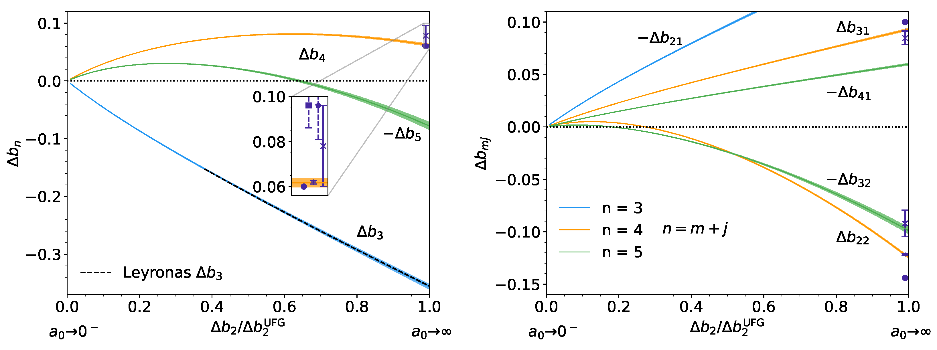
In Figure 1, we present the coefficients $\Delta b_k$ for $k=3,4,5$ (left panel) and the corresponding subspace contribution $\Delta b_{ij}$ (right panel). The inset on the left panel shows a comparison with experiments [51,52] and theory [36,39,47].

In addition to the excellent agreement with the $\Delta b_3$ results of Reference [33], the above provides a precise non-perturbative, non-stochastic determination of $\Delta b_4$ and $\Delta b_5$. The results show that, due to the competing subspace contributions (right panel), both $\Delta b_4$ and $\Delta b_5$ are non-monotonic as a function of the coupling strength. In addition, when approaching the unitary limit it is evident that $\Delta b_5$ becomes comparable in magnitude to $\Delta b_4$. It is this property that complicates the experimental determination of $\Delta b_4$ at strong coupling (dashed error bars in the inset of the left panel), as one is forced to assume that $\Delta b_5$ is comparatively small, which is not the case. The agreement for $\Delta b_4$ with the estimates of References [36,39,47], which use entirely different methods (among them and with the present work), further supports the accuracy and precision of the method. Note, however, the wide disparities in results for $\Delta b_{22}$ compared to $\Delta b_{31}$, which indicate that the $(2+2)$-particle subspace is a considerably more difficult problem to tackle than the polarized $(3+1)$ subspace.

5. Generalization to Other Systems

5.1. Harmonic Traps

Beyond the homogeneous system discussed above, systems in external harmonic traps are also of great interest [53,54] as a connection between theories (typically in homogeneous space) and the practical experimental realizations (which are to a good approximation in harmonic traps).

In the presence of harmonic traps, it is convenient to split the Hamiltonian into a non-interacting harmonic oscillator piece ${\widehat{H}}_0$, and the interaction $\widehat{V}$ in order to perform the Suzuki–Trotter factorization, such that

$$\widehat{H}={\widehat{H}}_0+\widehat{V},$$

(39)

where ${\widehat{H}}_0=\widehat{T}+{\widehat{V}}_{\mathrm{HO}}$ and

$${\widehat{V}}_{\mathrm{HO}}^{}=\int d^{3}r\frac{1}{2}m{\omega }^2{\mathbf{r}}^2\left[{\widehat{n}}_{\uparrow }^{}\left(\mathbf{r}\right)+{\widehat{n}}_{\downarrow }^{}\left(\mathbf{r}\right)\right],$$

(40)

is the harmonic trapping potential, and therefore

$$e^{-\tau \widehat{H}}=e^{-\tau {\widehat{H}}_0/2}{e}^{-\tau \widehat{V}}{e}^{-\tau {\widehat{H}}_0/2}+O\left({\tau }^3\right).$$

(41)

The main advantage of this choice of splitting of $\widehat{H}$ is that, as we will see below, the resulting factorization of the transfer matrices can be easily written in terms of the so-called Mehler kernel [15]. It should be pointed out that the other possible factorization where one combines ${\widehat{V}}_{\mathrm{HO}}$ with $\widehat{V}$ rather than with $\widehat{T}$ is an interesting possibility that one could explore entirely in momentum space (as in the homogeneous cases of the previous section). However, such an approach effectively results in a more complicated interaction made out of a one-body piece and a two-body piece with independent coupling constants, which must be kept track of throughout the calculation, with the concomitant increase in computational complexity. We will return to a similar situation below, namely the case of attractive Bose gases, which require two- and three-body forces for stability reasons.

As anticipated, the transfer matrices can be written conveniently in terms of the Mehler kernel. For example, when examining the $(1+1)$-particle subspace, we obtain

$$\begin{array}{ccc}\hfill {\mathcal{M}}_{11}& =& \langle {\mathbf{x}}_1,{\mathbf{x}}_2|e^{-\tau (\widehat{T}+{\widehat{V}}_{\mathrm{HO}}^{})}{e}^{-\tau \widehat{V}}|{\mathbf{y}}_1,{\mathbf{y}}_2\rangle \hfill \\ & =& \rho ({\mathbf{x}}_1,{\mathbf{y}}_1)\rho ({\mathbf{x}}_2,{\mathbf{y}}_2)\left[\mathbb{1}+C\delta ({\mathbf{y}}_1-{\mathbf{y}}_2)\right],\hfill \end{array}$$

(42)

where $\rho (\mathbf{x},\mathbf{y})$ is the Mehler kernel

$$\rho (\mathbf{x},\mathbf{y})=\frac{1}{{\lambda }_T^3}{\left[\frac{\beta \omega }{sinh\left(\tau \omega \right)}\right]}^{3/2}exp[-{\mathbf{Z}}^{T}B\mathbf{Z}],$$

(43)

which encodes the coordinate representation of the transfer matrix of a single-particle in the harmonic potential ${\widehat{V}}_{\mathrm{HO}}^{}$. Here, ${\mathbf{Z}}^T=({\mathbf{x}}^T/{\lambda }_T,{\mathbf{y}}^T/{\lambda }_T)$, and

$$\begin{array}{c}\hfill B=\frac{\pi \beta \omega }{sinh\left(\tau \omega \right)}\left(\begin{array}{cc}cosh\left(\tau \omega \right)\mathbb{1}& -\mathbb{1}\\ -\mathbb{1}& cosh\left(\tau \omega \right)\mathbb{1}\end{array}\right),\end{array}$$

(44)

where $\mathbb{1}$ is a $3\times 3$ unit matrix. Similarly, for the $(2+1)$-particle subspace, we find

$$\begin{array}{ccc}\hfill {\mathcal{M}}_{21}& =& \rho ({\mathbf{x}}_1,{\mathbf{y}}_1)\rho ({\mathbf{x}}_2,{\mathbf{y}}_2)\rho ({\mathbf{x}}_3,{\mathbf{y}}_3)\left\{\mathbb{1}+C[\delta ({\mathbf{y}}_1-{\mathbf{y}}_3)+\delta ({\mathbf{y}}_2-{\mathbf{y}}_3)]\right\}.\hfill \end{array}$$

(45)

Note that, as in a previous section, we do not include any symmetrization or antisymmetrization at this stage, as quantum statistics can be accounted for after the $N_{\tau }$-th power is taken. Further transfer matrices for up to five particles can be found in Reference [20].

As in the homogeneous case, we rely on known analytic results for $\Delta b_2$ in order to renormalize the interaction. In a harmonic trapping, potential $\Delta b_2^T$ is given at unitarity by [3]

$$\Delta b_2^T=\frac{1}{4}\mathrm{sech}\left(\frac{\beta \omega }{2}\right).$$

(46)

We note that, for arbitrary order, the trapped virial coefficients $\Delta b_n^T$ in the high-temperature (or low-frequency) limit $\beta \omega \to 0$ are connected with their homogeneous counterparts via

$$\Delta b_k=k^{3/2}\Delta b_k^T(\beta \omega \to 0),$$

(47)

which is useful to know when comparing homogeneous results with low-frequency extrapolations from the trapped case.

Using our framework at leading order ($N_{\tau }=1$) in d spatial dimensions, it is not difficult to obtain analytic formulas such as

$$\begin{array}{ccc}\hfill \Delta b_2& =& \Delta b_{11}=\frac{1}{2}\frac{C}{{\lambda }_T^d}{\left[\frac{\beta \omega }{2sinh\left(\beta \omega \right)}\right]}^{d/2},\hfill \end{array}$$

(48)

$$\begin{array}{ccc}\hfill \Delta b_{21}& =& -\frac{\Delta b_2}{{\left[2cosh\left(\beta \omega \right)+1\right]}^{d/2}},\hfill \end{array}$$

(49)

$$\begin{array}{ccc}\hfill \Delta b_{31}& =& \frac{2^{-d/2}\Delta b_2}{{cosh}^{d/2}\left(\beta \omega \right){\left[2cosh\left(\beta \omega \right)+1\right]}^{d/2}},\hfill \end{array}$$

(50)

and

$$\begin{array}{ccc}\hfill \Delta b_{22}& =& \frac{2^{-3d/2}\Delta b_2}{{cosh}^{d/2}\left(\beta \omega \right){cosh}^d(\beta \omega /2)}\times \hfill \\ & & \left\{1+2^{d/2}\Delta b_2\left[{cosh}^{d/2}\left(\beta \omega \right)-2^{d/2+1}{cosh}^d(\beta \omega /2)\right]\right\}.\hfill \end{array}$$

(51)

Following the same approach outlined in previous sections, we worked out the next-to-leading order ($N_{\tau }=2$) formulas, which the reader can find in Reference [20]. With automated algebra, these can be pushed to much higher $N_{\tau }$ to obtain estimates for $\Delta b_k$, which are then extrapolated to large $N_{\tau }$.

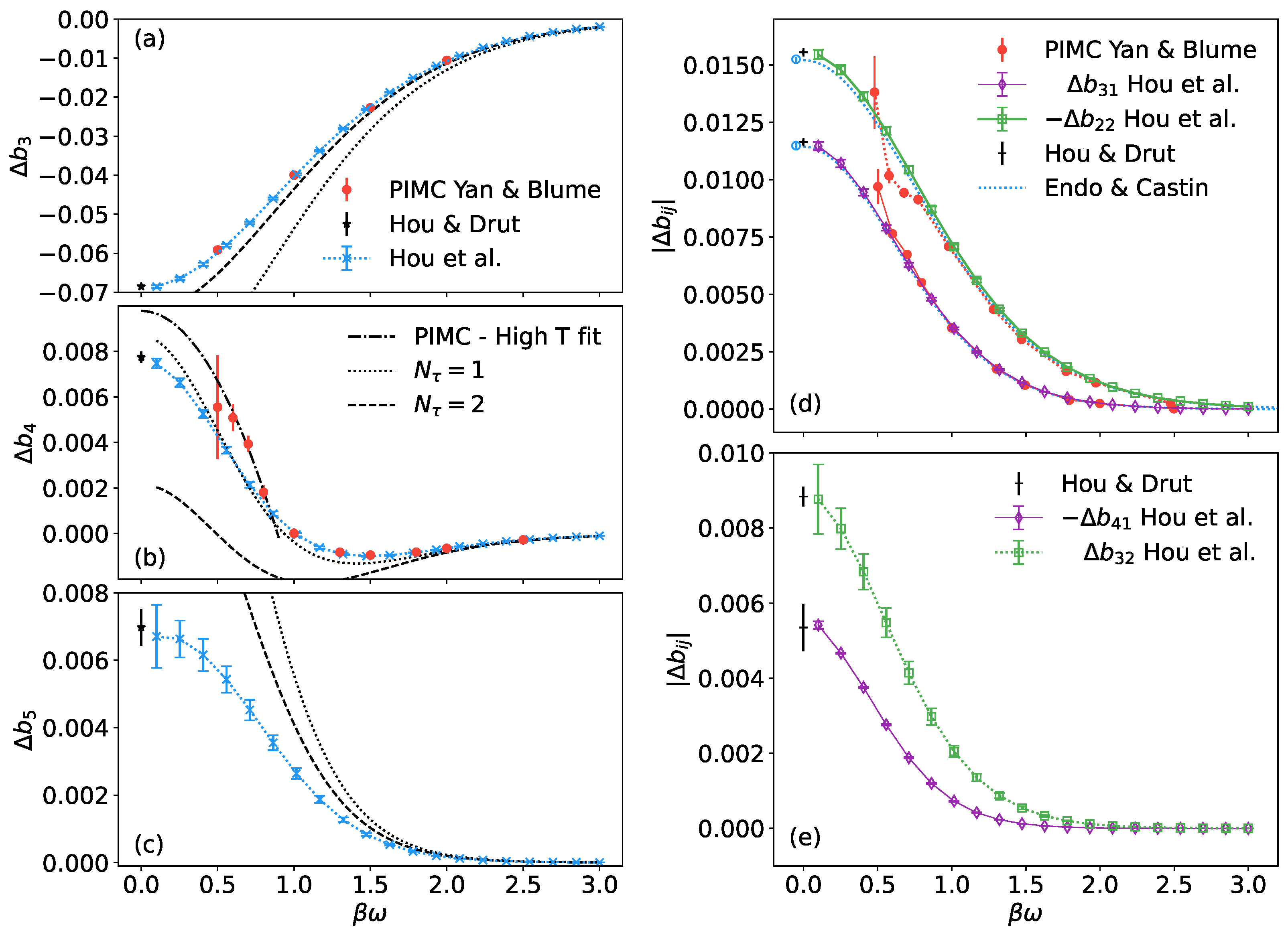
In Figure 2, we show our results at $N_{\tau }=1,2$ for the full-space contribution $\Delta b_k$, and those extrapolated to $N_{\tau }\to \infty$ limit for both $\Delta b_k$ and the corresponding subspace contribution $\Delta b_{ij}$. We find very good agreement between the extrapolated results and the Monte Carlo calculations of Reference [47] for large trapping frequency $\beta \omega$. As $\beta \omega$ approaches 0, our results are smoother compared to the Monte Carlo results, likely due to the volume cancellations that we are able to resolve analytically but which induce noise in the Monte Carlo method. Although the leading- and next-to-leading-order results deviate from the expected curve, they capture most qualitative features and may shed light on higher-order virial coefficients where the computational costs are too large for a full calculation at large $N_{\tau }$. Lastly, note that for $\Delta b_4$, the leading-order result is closer to the extrapolated curve compared to the next-leading-order result. This indicates that the discretization error from the Suzuki–Trotter decomposition is not monotonic in $N_{\tau }$. In other words, as $N_{\tau }$ increases, we may expect worse results before the asymptotic regime is approached. The onset of that regime is of course coupling dependent. Therefore, at a given interacting strength it is essential to investigate $N_{\tau }$ as high as possible in order to obtain quantitatively correct results.

5.2. Neutron Matter

The outermost crust of a neutron star is a low-density regime for which the unitary Fermi gas results presented above can be regarded as an approximation. To go beyond the unitary limit, a realistic model for neutron matter must include interaction range effects. In this section, we elaborate on a possible implementation of a finite-range interaction in the context of our method. To that end, we anticipate that it will be essential to expand the matrix elements of $e^{-\tau \widehat{V}}$ as a sum of Gaussians, as that would take advantage of the computational framework developed in the simpler cases discussed above.

As a reminder, for a contact interaction in the two-particle subspace, one has

$$\langle {\mathbf{q}}_1{\mathbf{q}}_2|e^{-\tau \widehat{V}}|{\mathbf{p}}_1{\mathbf{p}}_2\rangle ={\delta }_{{\mathbf{q}}_1,{\mathbf{p}}_1}{\delta }_{{\mathbf{q}}_2,{\mathbf{p}}_2}+C{\delta }_{{\mathbf{q}}_1+{\mathbf{q}}_2,{\mathbf{p}}_1+{\mathbf{p}}_2},$$

(52)

where C includes the lattice spacings and the bare coupling. Naturally, the first term represents a non-interacting piece and the second term encodes the interaction effects. A contact interaction in coordinate space has constant matrix elements in momentum space, but in the presence of a finite range there will be nontrivial momentum dependence, and therefore, we generalize the above via

$$C\to C({\mathbf{q}}_r,{\mathbf{p}}_r)=\sum _k{C}_k{e}^{-\tau {\lambda }_{1,k}({\mathbf{q}}_r^2+{\mathbf{p}}_r^2)+\tau {\lambda }_{2,k}{\mathbf{q}}_r·{\mathbf{p}}_r},$$

(53)

where ${\mathbf{q}}_r={\mathbf{q}}_1-{\mathbf{q}}_2$ and ${\mathbf{p}}_r={\mathbf{p}}_1-{\mathbf{p}}_2$. In the limit ${\lambda }_1,{\lambda }_2\to 0$, we reproduce the zero-range model. This type of expansion can be further generalized by including powers of ${\mathbf{q}}_r^2$, ${\mathbf{p}}_r^2$ and ${\mathbf{q}}_r·{\mathbf{p}}_r$ as a prefactor rather than in the exponent, which can be used to account for more features of the interaction. However, such a generalization should be used sparingly or not at all if possible, as it would dramatically (specifically, factorially) increase the number of terms that result in the expansion, by virtue of Wick’s theorem.

5.3. Unitary Bose Gas

The case of Bose gases with attractive interactions, in particular close to the universal regime of the unitary limit, requires special care. Given the absence of Pauli exclusion, attractively interacting bosons undergo Thomas collapse [55], i.e., they are unstable. Moreover, close to unitarity, they display the Efimov effect [56,57]. To properly renormalize such a system, a repulsive three-body interaction is required [58]. The latter introduces a new dimensionful parameter that is sensitive to the ultraviolet cutoff and must be fixed by using some known physical quantity.

To account for the above, we consider an interaction of the form

$$\widehat{V}=-\frac{g_2}{2!}\sum _{\mathbf{r}}{\left(a_{\mathbf{r}}^{†}\right)}^2{\left({\widehat{a}}_{\mathbf{r}}^{}\right)}^2-\frac{g_3}{3!}\sum _{\mathbf{r}}{\left({\widehat{a}}_{\mathbf{r}}^{†}\right)}^3{\left({\widehat{a}}_{\mathbf{r}}^{}\right)}^3,$$

(54)

where we have used the normal-ordered form and ${\widehat{a}}_{\mathbf{r}}^{†}$, ${\widehat{a}}_{\mathbf{r}}^{}$ are the bosonic creation and annihilation operators at point $\mathbf{r}$.

In previous sections, we used $\Delta b_2$ to renormalize a two-body contact interaction. It is, therefore, natural in the present case to use $\Delta b_2$ and $\Delta b_3$ for the same purpose. Since $\Delta b_2$ involves only the two-particle subspace, we use it to renormalize the two-body interaction in the usual way before proceeding to $\Delta b_3$, which depends on both the two- and three-particle subspaces and thus determines the three-body coupling. In the bosonic unitary limit, the three-body parameter induces a temperature dependence on $\Delta b_3$, which was calculated exactly in Reference [59].

Calculating $\Delta b_2$ using the above interaction in d spatial dimensions and $N_{\tau }=1$, we obtain

$$\Delta b_2=\frac{\Delta Q_2}{Q_1}=\beta g_2\frac{Q_1}{V},$$

(55)

where $V=L^d$ is the d-dimensional volume, such that in the (spatial) continuum limit

$$\Delta b_2\to \frac{1}{2\pi }\frac{g_2}{{\lambda }_T^{d-2}},$$

(56)

where we used that in that limit $Q_1/V\to {\lambda }_T^{-d}$.

On the other hand, a calculation of $\Delta b_3$, also in d spatial dimensions and $N_{\tau }=1$, yields

$$\Delta b_3=\frac{\Delta Q_3}{Q_1}-Q_1\Delta b_2=\frac{\beta g_2}{2!}4\frac{Q_1\left(2\beta \right)}{V}+\frac{\beta g_3}{3!}6\frac{Q_1^2}{V^2},$$

(57)

which in the (spatial) continuum limit becomes

$$\Delta b_3\to \frac{1}{2^{d/2-1}}\frac{1}{2\pi }\frac{g_2}{{\lambda }_T^{d-2}}+\frac{3}{\pi }\frac{g_3}{{\lambda }_T^{2d-2}}.$$

(58)

We thus see that, as anticipated, $\Delta b_2$ and $\Delta b_3$ determine $g_2$ and $g_3$. At the $N_{\tau }=1$ level of this calculation, the temperature dependence of $\Delta b_2$ and $\Delta b_3$ will typically induce a temperature dependence in $g_2$ and $g_3$. More explicitly, we may invert the above results to obtain the dimensionless form

$$\begin{array}{ccc}\hfill \beta g_2{\lambda }_T^{-d}& =& \Delta b_2,\hfill \end{array}$$

(59)

$$\begin{array}{ccc}\hfill \beta g_3{\lambda }_T^{-2d}& =& \Delta b_3-\frac{1}{2^{d/2-1}}\Delta b_2.\hfill \end{array}$$

(60)

Armed with these answers, the renormalization program is complete and we may proceed to calculate and predict higher-order virial coefficients. Our leading order ($N_{\tau }=1$) for the fourth-order bosonic virial coefficient $\Delta b_4$ is neatly expressed in terms of a relationship with $\Delta b_2$ and $\Delta b_3$:

$$\Delta b_4=\left(3^{-d/2}2+2^{-d}-\frac{3}{2^{d-1}}\right)\Delta b_2+\left(2^{-d/2+1}+2^{-2d-1}\right){\left(\Delta b_2\right)}^2+\frac{3}{2^{d/2}}\Delta b_3.$$

(61)

In Figure 3, we show the above result applied to $d=3$ at unitarity, where $\Delta b_2=\sqrt{2}$ and $\Delta b_3$ is as determined in Reference [59]. Our $N_{\tau }=1$ approximation is likely a rather crude one, but it should be asymptotically correct for small $\beta E_T$.

6. Pressure, Density, and Generalization to Other Observables

Thus far, we limited our scope to the expansion for pressure, but the virial expansion is much more general and can be applied to a wide range of observables. In this section, we present the generalization of our approach to the Tan contact, the momentum distribution, and the structure factor.

6.1. From Pressure to Density and Tan Contact

By way of the grand thermodynamic potential, the $b_n$ grants access to all thermodynamic quantities, at least in principle. One of the most basic quantities besides the pressure is the density, which is given by

$$n=\frac{ln\mathcal{Z}}{lnz}=n_0+\frac{2}{{\lambda }_T^d}\sum _{k=2}^{\infty }m\Delta b_k{z}^k,$$

(62)

where $n_0$ is the density at the absence of interaction, and similarly in the presence of finite polarization (i.e., different fugacities $z_{\uparrow }$ and $z_{\downarrow }$ for each spin),

$$n_s=n_{s,0}+\frac{2}{{\lambda }_T^d}\sum _{k=2}^{\infty }\sum _{\begin{array}{c}i,j>0\\ i+j=k\end{array}}[i{\delta }_{s,\uparrow }+j{\delta }_{s,\downarrow }]\Delta b_{ij}{z}_{\uparrow }^i{z}_{\downarrow }^j,$$

(63)

where $s=\uparrow ,\downarrow$ for each spin.

Beyond global thermodynamic quantities, the Tan contact can also be investigated through the virial expansion (see, e.g., Reference [54]). For systems with short-range two-body forces, the Tan contact represents the probability of finding two particles at the same spatial location. For that reason, it captures the short-distance behavior of all correlation functions. In particular, the momentum distribution in such systems decays at large momentum k as

$$n\sim \mathcal{I}/k^4,$$

(64)

where $\mathcal{I}$ is the contact. Thus, one way to measure or calculate the contact is to determine the large-momentum tail of the momentum distribution. In practice, however, it has proven more efficient to use the so-called adiabatic relation, whereby $\mathcal{I}$ is obtained from the variation of the grand thermodynamic potential with the coupling strength.

In Tan’s original works [11,12,13], he considered a Fermi gas in 3D. Later works further developed the theory and extended it to one [60] and two [61] dimensions, as well as bosonic systems [62,63,64].

Below we focus on the three-dimensional Fermionic system, but readers are referred to Reference [19] for more details on one- and two- dimensional Fermi gas.

In three spatial dimensions, the VE for the contact is obtained via

$$\mathcal{I}=-\frac{4\pi }{\beta }\frac{\partial (\beta \Omega )}{\partial a_0^{-1}}=\frac{4\pi }{\sqrt{\beta }}\frac{\partial ln\mathcal{Z}}{\partial \lambda }=\frac{4\pi }{\beta }{Q}_1{\lambda }_T\sum _{k=2}^{\infty }{c}_k{z}^k,$$

(65)

where

$$c_k=\frac{1}{\sqrt{2\pi }}\frac{\partial \Delta b_k}{\partial \lambda },$$

(66)

are the virial coefficients of $\mathcal{I}$. To evaluate the partial derivative, the most straightforward method is to apply the chain rule as

$$\begin{array}{c}\hfill \frac{\partial \Delta b_k}{\partial \lambda }=\frac{\partial \Delta b_k}{\partial \Delta b_2}\frac{\partial \Delta b_2}{\partial \lambda },\end{array}$$

(67)

where the first derivative can be calculated numerically, and the second is analytically given by the Beth–Uhlenbeck formula as

$$\frac{\partial \Delta b_2}{\partial \lambda }=\sqrt{\frac{2}{\pi }}+\sqrt{2}\lambda e^{{\lambda }^2}[1+\mathrm{erf}\left(\lambda \right)].$$

(68)

Thanks to the analytical nature of our method, one can improve the accuracy of the numerical derivative without repeating calculations. Alternatively, one can take advantage of the analytic form of $\Delta b_k$ from our method, which is a polynomial in terms of coupling strength C

$$\Delta b_k=\sum _{l=1}^{l_{\max }}{A}_l{C}^l,$$

(69)

where $l_{\max }=min(M,N)·N_{\tau }$ is the degree of the polynomial. The derivative can then be treated as a polynomial in C of degree $l_{\max }-1$ as

$$\frac{\partial \Delta b_k}{\partial \lambda }=\sum _{l=1}^{l_{\max }}l·A_l{C}^{l-1}\frac{\partial C}{\partial \lambda }=\sum _{l=1}^{l_{\max }}{B}_l\left(D\right)C^{l-1},$$

(70)

where $D=\frac{\partial C}{\partial l}$ and $B_l\left(D\right)=l{A}_{l}D$. Now, we treat C and D as two independent variables and tune their values in two passes: firstly, the value of C is renormalized to reproduce the $\Delta b_2$; and then we plug the resulting C in Equation (70) and tune D to produce the expected second-order result, as given in Equation (68).

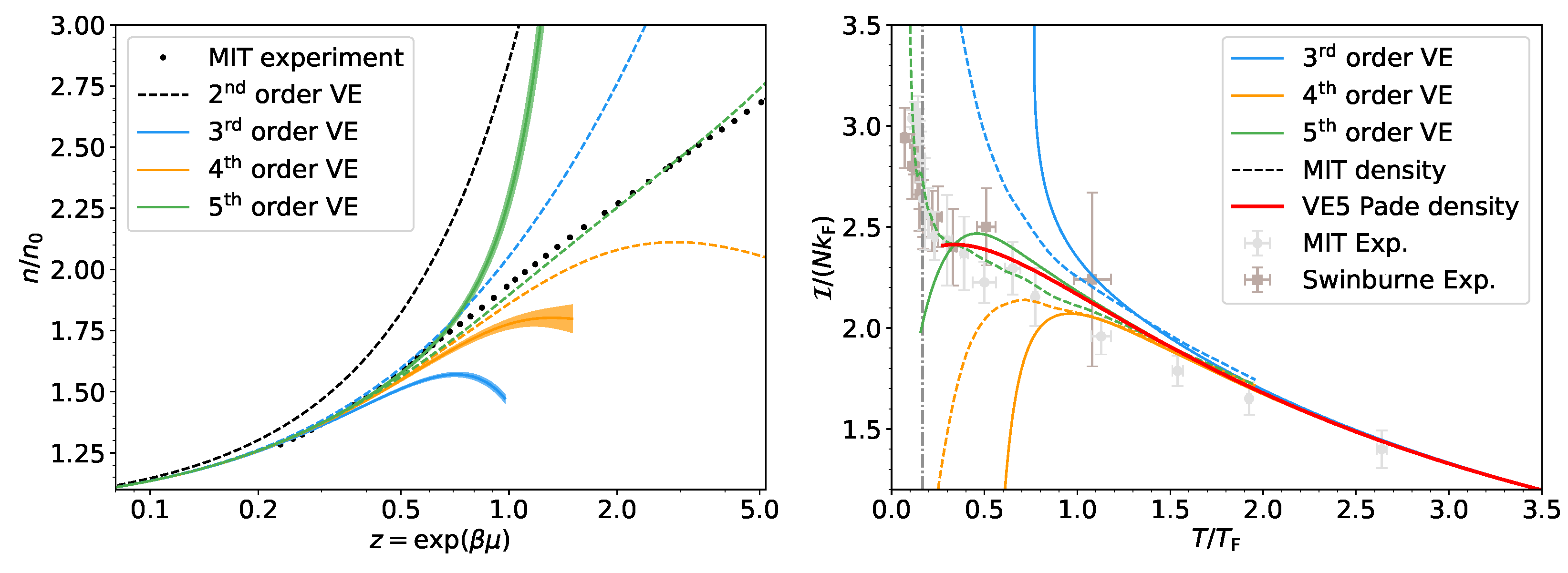
In Figure 4, we plot the density (left panel) and Tan contact (right panel) in the homogeneous case. On the left panel, the solid lines (with uncertainty bands) are the results of using the VE at face value, i.e., truncated at a given order: blue for third order, red for fourth-order, and green for fifth-order. In each case, a corresponding dashed line of the same color shows the results of Padé resummation at that order. Across this work, we used either the diagonal or off-diagonal Padé resummation, i.e., the order usually denoted as $[a/b]$ satisfies $a=b$ (diagonal) or $a+1=b$ (off-diagonal). Finally, the second-order results are shown as a black dashed line for reference, while the black dots come from the MIT experiment of Reference [52]. For both the truncated VE and the resummed results, we found improved agreement as higher-order contributions were included, the effect being most notable when the resummation is applied. This inspires an open question under investigation on the effect of the resummation when using even higher orders. This is particularly intriguing as access to higher-order coefficients would allow more freedom in exploring a range of resummation techniques.

In the right panel of Figure 4, we show the dimensionless contact in the form

$$\frac{\mathcal{I}}{N{k}_F}=3{\pi }^2{\left(\frac{T}{T_F}\right)}^2\sum _{k=2}{c}_k{z}^k,$$

(71)

as a function of the reduced temperature $T/T_F$, which is related to the density via

$${\left(\frac{T}{T_F}\right)}^3={\left(\frac{8}{3\sqrt{\pi }{\lambda }_T^{3}n}\right)}^2.$$

(72)

Therefore, the resulting curve is an interplay between two independent series for the density and the contact. In particular, the curve will be more sensitive to the density estimate as both quantities implicitly depend on it. In other words, in the region where we observed deviation in the left panel between our results and experimental determinations, we expect errors in both horizontal and vertical directions. This approximately corresponds to $z⪆0.75$, or $T/T_F⪅1.4$, for the truncated VE results. At higher temperatures, where our results coincide with the experimental measurement, the main source of error is the expansion series for $\mathcal{I}$.

To better show $\mathcal{I}$, as given in Equation (65), and isolate the influence on the density, we use the experimental values [65] (see also Refs. [66,67,68] for relevant experimental studies) to calculate the reduced temperature $T/T_F$ (thus providing an essentially exact density) and evaluate the series ${\sum }_{k=2}^{\infty }{c}_k{z}^k$ using Padé resummation at different orders (dashed lines). Overall, we observed the same trend as for the density where the results are improved as higher-order contributions are included. Although the resummed fifth-order VE (red dashed line) seems to give very good results below the critical temperature, one should take such an agreement with a grain of salt, as the error in the dimensionless contact is greatly reduced by a factor of ${(T/T_F)}^2$. Furthermore, this result is free from errors in the density because we have used the experimental data for the latter.

To represent the more practical situation where we have no access to accurate experimental measurement of the density, we use the best density estimate (green dashed line in the left panel), and the final result is plotted as the thick red solid line. Even though the approximation begins to fail when approaching the critical temperature, we find impressive agreement until $T/T_F\approx 0.4$, roughly corresponding to the diverging point between the Padé and experimental results at $z=5.0$ for the density.

Figure 4. (Left): Density $n/n_0$ as a function of fugacity z. The colorful solid lines are the results using truncated VE at third (blue), fourth (orange) and fifth (green) order. The black dashed line is the result using second-order VE. The dashed lines are the results using diagonal or off-diagonal Padé resummation. The black dotted line is the experimental measurement by Reference [52]. (Right): Dimensionless contact $\mathcal{I}/\left(N{k}_F\right)$ as a function of reduced temperature $T/T_F$. The blue, orange and green solid lines are the results using truncated VE for both the contact and the density, which is connected to the reduced temperature $T/T_F$. The same color code is used. Colorful dotted lines are the results using the experimental density measurement and VE contact. The red curves are the results using resummation: the dotted is with experimental density and the solid with Padé resummed density. The light gray and brown points are experimental determinations from Reference [65] and Reference [69], respectively.

Figure 4. (Left): Density $n/n_0$ as a function of fugacity z. The colorful solid lines are the results using truncated VE at third (blue), fourth (orange) and fifth (green) order. The black dashed line is the result using second-order VE. The dashed lines are the results using diagonal or off-diagonal Padé resummation. The black dotted line is the experimental measurement by Reference [52]. (Right): Dimensionless contact $\mathcal{I}/\left(N{k}_F\right)$ as a function of reduced temperature $T/T_F$. The blue, orange and green solid lines are the results using truncated VE for both the contact and the density, which is connected to the reduced temperature $T/T_F$. The same color code is used. Colorful dotted lines are the results using the experimental density measurement and VE contact. The red curves are the results using resummation: the dotted is with experimental density and the solid with Padé resummed density. The light gray and brown points are experimental determinations from Reference [65] and Reference [69], respectively.

6.2. One-Body Operator Example: The Momentum Distribution

In addition to the density and pressure equations of state, the next simplest quantity one can calculate is the expectation value of a one-body operator; for instance, the momentum distribution ${\widehat{n}}_{\sigma }\left(\mathbf{p}\right)$ of particles with spin $\sigma$. Of course, here the only added difficulty is that the operator singles out a specific momentum $\mathbf{p}$, but it warrants special attention.

The starting point is the thermal expectation value

$$\langle {\widehat{n}}_{\sigma }\left(\mathbf{p}\right)\rangle =\frac{1}{\mathcal{Z}}\mathrm{Tr}\left[e^{-\beta (\widehat{H}-\mu \widehat{N})}{\widehat{n}}_{\sigma }\left(\mathbf{p}\right)\right].$$

(73)

Having available the virial expansion for $\mathcal{Z}$ already, we focus on the numerator

$$\mathrm{Tr}\left[e^{-\beta (\widehat{H}-\mu \widehat{N})}{\widehat{n}}_{\sigma }\left(\mathbf{p}\right)\right]=\sum _{N=1}^{\infty }{\mathrm{tr}}_N^{}\left[e^{-\beta \widehat{H}}{\widehat{n}}_{\sigma }\left(\mathbf{p}\right)\right]z^N,$$

(74)

Thus, after expanding the denominator $\mathcal{Z}$,

$$\langle {\widehat{n}}_{\sigma }\left(\mathbf{p}\right)\rangle =\sum _{k=1}^{\infty }{m}_{\sigma ,k}\left(\mathbf{p}\right)z^k,$$

(75)

where

$$\begin{array}{ccc}\hfill m_{\sigma ,1}\left(\mathbf{p}\right)& =& {\mathrm{tr}}_1^{}\left[e^{-\beta \widehat{H}}{\widehat{n}}_{\sigma }\left(\mathbf{p}\right)\right],\hfill \end{array}$$

(76)

$$\begin{array}{ccc}\hfill m_{\sigma ,2}\left(\mathbf{p}\right)& =& {\mathrm{tr}}_2^{}\left[e^{-\beta \widehat{H}}{\widehat{n}}_{\sigma }\left(\mathbf{p}\right)\right]-Q_1{\mathrm{tr}}_1^{}\left[e^{-\beta \widehat{H}}{\widehat{n}}_{\sigma }\left(\mathbf{p}\right)\right],\hfill \end{array}$$

(77)

$$\begin{array}{ccc}\hfill m_{\sigma ,3}\left(\mathbf{p}\right)& =& {\mathrm{tr}}_3^{}\left[e^{-\beta \widehat{H}}{\widehat{n}}_{\sigma }\left(\mathbf{p}\right)\right]-Q_1{\mathrm{tr}}_2^{}\left[e^{-\beta \widehat{H}}{\widehat{n}}_{\sigma }\left(\mathbf{p}\right)\right]\hfill \end{array}$$

(78)

$$\begin{array}{ccc}& & +\left(Q_1^2-Q_2\right){\mathrm{tr}}_1^{}\left[e^{-\beta \widehat{H}}{\widehat{n}}_{\sigma }\left(\mathbf{p}\right)\right],\hfill \end{array}$$

(79)

and so forth. (Note that, naturally, the content of $m_{\sigma ,1}\left(\mathbf{k}\right)$ is entirely non-interacting, as it corresponds to a single-particle subspace.)

The new “virial coefficients” $m_{\sigma ,k}\left(\mathbf{p}\right)$ require the calculation of the Hilbert trace ${\mathrm{tr}}_N\left[e^{-\beta \widehat{H}}{\widehat{n}}_{\sigma }\left(\mathbf{p}\right)\right]$, denoted as $W_N\left[{\widehat{n}}_{\sigma }\left(\mathbf{p}\right)\right]$ or just $W_{N,\sigma }$ for shorthand. In our method, its evaluation shares the same formalism as the usual partition function $Q_N$ as in Equation (31) and (32), i.e., the trace $W_{N,\sigma }$ encodes the particle statistics. Taking the $(2,1)$-system for example,

$$\begin{array}{cc}\hfill W_{21,\sigma }^{\mathrm{F}}& ={\mathrm{tr}}_{\mathrm{F}}^{}\left[{\mathcal{M}}_{21}^{N_{\tau }}{\mathcal{N}}_{21,\sigma }\left(\mathbf{p}\right)\right]=\frac{1}{2!}\sum _{abc}\left\{{\left[{\mathcal{M}}_{21}^{N_{\tau }}{\mathcal{N}}_{21,\sigma }\left(\mathbf{p}\right)\right]}_{abc,abc}-{\left[{\mathcal{M}}_{21}^{N_{\tau }}{\mathcal{N}}_{21,\sigma }\left(\mathbf{p}\right)\right]}_{abc,bac}\right\},\hfill \\ \hfill W_{21,\sigma }^{\mathrm{B}}& ={\mathrm{tr}}_{\mathrm{B}}^{}\left[{\mathcal{M}}_{21}^{N_{\tau }}{\mathcal{N}}_{21,\sigma }\left(\mathbf{p}\right)\right]=\frac{1}{2!}\sum _{abc}\left\{{\left[{\mathcal{M}}_{21}^{N_{\tau }}{\mathcal{N}}_{21,\sigma }\left(\mathbf{p}\right)\right]}_{abc,abc}+{\left[{\mathcal{M}}_{21}^{N_{\tau }}{\mathcal{N}}_{21,\sigma }\left(\mathbf{p}\right)\right]}_{abc,bac}\right\}.\hfill \end{array}$$

(80)

where ${\mathcal{N}}_{\sigma ,\mathbf{p}}$ is the matrix elements of momentum density operator

$$\begin{array}{cc}\hfill {\mathcal{N}}_{21,\sigma }\left(\mathbf{p}\right)& =\langle {\mathbf{p}}_1{\mathbf{p}}_2{\mathbf{p}}_3|{\widehat{n}}_{\sigma }\left(\mathbf{p}\right)|{\mathbf{q}}_1{\mathbf{q}}_2{\mathbf{q}}_3\rangle \hfill \\ \hfill & =\left[{\delta }_{\mathbf{p}{\mathbf{p}}_1}+{\delta }_{\mathbf{p}{\mathbf{p}}_2}\right]\langle {\mathbf{p}}_1{\mathbf{p}}_2{\mathbf{p}}_3|{\mathbf{q}}_1{\mathbf{q}}_2{\mathbf{q}}_3\rangle \hfill \\ \hfill & =\left[{\delta }_{\mathbf{p}{\mathbf{p}}_1}+{\delta }_{\mathbf{p}{\mathbf{p}}_2}\right]{\delta }_{{\mathbf{p}}_1{\mathbf{q}}_1}{\delta }_{{\mathbf{p}}_2{\mathbf{q}}_2}{\delta }_{{\mathbf{p}}_3{\mathbf{q}}_3}.\hfill \end{array}$$

(81)

At the leading-order up to the third-order in fugacity, we obtain the change of momentum distribution with respect to that in the non-interacting case,

$$\Delta n_{\sigma }\left(\mathbf{p}\right)=\frac{C}{{\lambda }_T^d}exp(-\frac{d}{4\pi }{\tilde{k}}^2)z^2-4\frac{C}{{\lambda }_T^d}exp(-\frac{d}{2\pi }{\tilde{k}}^2)z^3,$$

(82)

where $\tilde{k}={\lambda }_{T}k$ is the dimensionless momentum. As in previous cases, we emphasize that this is merely an approximation at the lowest nontrivial order in C, but it provides a qualitative guide and a reasonable answer at weak coupling.

6.3. Two-Body Operators and Real-Time Evolution

An advantage of our automated algebra method is its versatility. The formalism and implementation can be adapted to more complicated observables without introducing significant new complexity. In this section, we present the first steps for a few such examples, which show the way for future work.

As a natural extension of the case of one-body operators, Equation (74) is generalized to two-body operators:

$$\begin{array}{cc}\hfill \langle {\widehat{O}}_1{\widehat{O}}_2\rangle & =\frac{1}{\mathcal{Z}}\mathrm{Tr}\left[e^{-\beta (\widehat{H}-\mu \widehat{N})}{\widehat{O}}_1{\widehat{O}}_2\right]\hfill \\ \hfill & =\frac{1}{\mathcal{Z}}\sum _{N=1}^{\infty }{\mathrm{tr}}_N[e^{-\beta \widehat{H}}{\widehat{O}}_1{\widehat{O}}_2]z^N.\hfill \end{array}$$

(83)

From this point on, the evaluation of the N-particle Hilbert space trace $W({\widehat{O}}_1,{\widehat{O}}_2)={\mathrm{tr}}_N[e^{-\beta \widehat{H}}{\widehat{O}}_1{\widehat{O}}_2]$ follows the same methodology explained in the previous section.

An interesting two-body quantity is the density–density correlation $\langle \widehat{n}\left(\mathbf{r}\right)\widehat{n}\left(0\right)\rangle$, which is the central ingredient of the static structure factor:

$$S\left(q\right)=\int d^{3}r{e}^{-i\mathbf{q}·\mathbf{r}}\langle \delta \widehat{n}\left(\mathbf{r}\right)\delta \widehat{n}\left(0\right)\rangle$$

(84)

where $\delta \widehat{X}=\widehat{X}-\langle \widehat{X}\rangle$. The latter approximately describes the in-medium scattering rate in certain contexts [70]. Recent studies [71,72] examined this quantity within the VE up to second order, and it is interesting to examine the effect of higher-order contributions. Yet another example that has been intensely investigated recently is the viscosity. Specifically, in the work of References [73,74,75], the VE was applied to the calculation of both bulk and shear viscosity, which requires the commutator of the contact operator.

Our formalism can also be generalized beyond equilibrium systems by including real-time evolution. The recent work of Reference [76] investigated the effects of an interaction quench in a bosonic system, in an attempt to explain the results of the experiment of Reference [77]. Here, the system starts as non-interacting and in thermal equilibrium, and then an interparticle interaction is suddenly switched on. The process was investigated in Reference [76] using the VE of the momentum distribution $n\left(k\right)$ up to second order, and varying behaviors at low and high momenta k were found. Although this is an interesting result, the effect of higher-order contributions remains an open problem and may not be small, which further motivates the extension of our framework for more general dynamic processes.

The quench process mentioned above is described by the Hamiltonian

$$\widehat{H}={\widehat{H}}_0+\Theta \left(t\right)\widehat{V},$$

(85)

where ${\widehat{H}}_0$ is the free Hamiltonian and $\widehat{V}$ is the interaction, which is turned on at $t=0$. To study the evolution of a given operator $\widehat{O}$ one starts with expressions similar to Equation (83), with the exception that the Hilbert space trace now becomes time-dependent

$$W_N(\widehat{O},t)={\mathrm{tr}}_N(e^{-\beta \widehat{H_0}}{e}^{it\widehat{H}}\widehat{O}{e}^{-it\widehat{H}}).$$

(86)

Research regarding the investigation of these kinds of expressions with automated algebra, specifically for the interaction quench, is underway.

7. Summary and Conclusions

The VE is an expansion of the quantum many-body thermodynamics in powers of the fugacity z that is capable of non-perturbatively characterizing such many-body systems in dilute, high-temperature regimes. The challenge of the VE is that calculating its coefficients $b_k$ at n-th order in the expansion requires analyzing the quantum n-body problem in some detail.

In this brief review, we have outlined some of the main methods used to calculate $b_k$ and advocated for an approach based on discretizing imaginary time, thus obtaining a factorized transfer matrix, and automating the resulting algebra to calculate the trace of the $N_{\tau }$-th power of the transfer matrix. We have shown in detail how such a method is structured and how it is able to provide reliable results for up to $b_5$ for strongly coupled nonrelativistic fermions, focusing on the unitary limit. The automated algebra algorithm is fully parallelizable and may thus be extended beyond $b_5$ with increased computational power.

We have also shown how to generalize the approach to account for harmonic trapping potentials, neutron matter and attractive Bose gases (which require three-body forces). Furthermore, the method is also straightforwardly generalized to observables other than the pressure, such as the Tan contact, the momentum distribution, and the structure factor.

References

- Berger, C.; Rammelmueller, L.; Loheac, A.; Ehmann, F.; Braun, J.; Drut, J. Complex Langevin and other approaches to the sign problem in quantum many-body physics. Phys. Rep. 2021, 892, 1–54. [Google Scholar] [CrossRef]
- Pathria, R. Statistical Mechanics; International Series of Monographs in Natural Philosophy; Elsevier Science & Technology Books: Amsterdam, The Netherlands, 1972. [Google Scholar]
- Liu, X.J. Virial expansion for a strongly correlated Fermi system and its application to ultracold atomic Fermi gases. Phys. Rep. 2013, 524, 37–83. [Google Scholar] [CrossRef] [Green Version]
- Mayer, J.E.; Mayer, M.G. Statistical Mechanics; John Wiley and Sons, Inc.: New York, NY, USA, 1940. [Google Scholar]
- Kahn, B.; Uhlenbeck, G.E. On the theory of condensation. Physica 1938, 5, 399. [Google Scholar] [CrossRef]
- Lee, T.D.; Yang, C.N. Many-Body Problem in Quantum Statistical Mechanics. I. General Formulation. Phys. Rev. 1959, 113, 1165. [Google Scholar] [CrossRef]
- Lee, T.D.; Yang, C.N. Many-Body Problem in Quantum Statistical Mechanics. II. Virial Expansion for Hard-Sphere Gas. Phys. Rev. 1959, 116, 25. [Google Scholar] [CrossRef]
- Lee, T.D.; Yang, C.N. Many-Body Problem in Quantum Statistical Mechanics. III. Zero-Temperature Limit for Dilute Hard Spheres. Phys. Rev. 1960, 117, 12. [Google Scholar] [CrossRef]
- Lee, T.D.; Yang, C.N. Many-Body Problem in Quantum Statistical Mechanics. IV. Formulation in Terms of Average Occupation Number in Momentum Space. Phys. Rev. 1960, 117, 22. [Google Scholar] [CrossRef]
- Lee, T.D.; Yang, C.N. Many-Body Problem in Quantum Statistical Mechanics. V. Degenerate Phase in Bose-Einstein Condensation. Phys. Rev. 1960, 117, 897. [Google Scholar] [CrossRef]
- Tan, S. Energetics of a strongly correlated Fermi gas. Ann. Phys. 2008, 323, 2952–2970. [Google Scholar] [CrossRef] [Green Version]
- Tan, S. Large momentum part of a strongly correlated Fermi gas. Ann. Phys. 2008, 323, 2971–2986. [Google Scholar] [CrossRef] [Green Version]
- Tan, S. Generalized virial theorem and pressure relation for a strongly correlated Fermi gas. Ann. Phys. 2008, 323, 2987–2990. [Google Scholar] [CrossRef] [Green Version]
- Shill, C.R.; Drut, J.E. Virial coefficients of one-dimensional and two-dimensional Fermi gases by stochastic methods and a semiclassical lattice approximation. Phys. Rev. A 2018, 98, 053615. [Google Scholar] [CrossRef] [Green Version]
- Morrell, K.J.; Berger, C.E.; Drut, J.E. Third- and fourth-order virial coefficients of harmonically trapped fermions in a semiclassical approximation. Phys. Rev. A 2019, 100, 063626. [Google Scholar] [CrossRef] [Green Version]
- Hou, Y.; Czejdo, A.J.; DeChant, J.; Shill, C.R.; Drut, J.E. Leading- and next-to-leading-order semiclassical approximation to the first seven virial coefficients of spin-1/2 fermions across spatial dimensions. Phys. Rev. A 2019, 100, 063627. [Google Scholar] [CrossRef] [Green Version]
- Czejdo, A.J.; Drut, J.E.; Hou, Y.; McKenney, J.R.; Morrell, K.J. Virial coefficients of trapped and untrapped three-component fermions with three-body forces in arbitrary spatial dimensions. Phys. Rev. A 2020, 101, 063630. [Google Scholar] [CrossRef]
- Hou, Y.; Drut, J.E. Fourth- and Fifth-Order Virial Coefficients from Weak Coupling to Unitarity. Phys. Rev. Lett. 2020, 125, 050403. [Google Scholar] [CrossRef]
- Hou, Y.; Drut, J.E. Virial expansion of attractively interacting Fermi gases in one, two, and three dimensions, up to fifth order. Phys. Rev. A 2020, 102, 033319. [Google Scholar] [CrossRef]
- Hou, Y.; Morrell, K.J.; Czejdo, A.J.; Drut, J.E. Fourth- and fifth-order virial expansion of harmonically trapped fermions at unitarity. Phys. Rev. Res. 2021, 3, 033099. [Google Scholar] [CrossRef]
- Rammelmueller, L.; Hou, Y.; Drut, J.E.; Braun, J. Pairing and the spin susceptibility of the polarized unitary Fermi gas in the normal phase. Phys. Rev. A 2021, 103, 043330. [Google Scholar] [CrossRef]
- Uhlenbeck, G.E.; Beth, E. The quantum theory of the non-ideal gas I. Deviations from the classical theory. Physica 1936, 3, 729–745. [Google Scholar] [CrossRef]
- Beth, E.; Uhlenbeck, G.E. The quantum theory of the non-ideal gas. II. Behaviour at low temperatures. Physica 1937, 4, 915–924. [Google Scholar] [CrossRef]
- Hoffman, M.D.; Javernick, P.D.; Loheac, A.C.; Porter, W.J.; Anderson, E.R.; Drut, J.E. Universality in one-dimensional fermions at finite temperature: Density, pressure, compressibility, and contact. Phys. Rev. A 2015, 91, 033618. [Google Scholar] [CrossRef] [Green Version]
- Loheac, A.C.; Drut, J.E. Third-order perturbative lattice and complex Langevin analyses of the finite-temperature equation of state of nonrelativistic fermions in one dimension. Phys. Rev. D 2017, 95, 094502. [Google Scholar] [CrossRef] [Green Version]
- Chafin, C.; Schäfer, T. Scale breaking and fluid dynamics in a dilute two-dimensional Fermi gas. Phys. Rev. A 2013, 88, 043636. [Google Scholar] [CrossRef] [Green Version]
- Daza, W.; Drut, J.E.; Lin, C.; Ordóñez, C. Virial expansion for the Tan contact and Beth-Uhlenbeck formula from two-dimensional SO(2,1) anomalies. Phys. Rev. A 2018, 97, 033630. [Google Scholar] [CrossRef] [Green Version]
- Lee, D.; Schäfer, T. Cold dilute neutron matter on the lattice. I. Lattice virial coefficients and large scattering lengths. Phys. Rev. C 2006, 73, 015201. [Google Scholar] [CrossRef] [Green Version]
- Horowitz, C.; Schwenk, A. The virial equation of state of low-density neutron matter. Phys. Lett. B 2006, 638, 153–159. [Google Scholar] [CrossRef] [Green Version]
- Horowitz, C.; Schwenk, A. Cluster formation and the virial equation of state of low-density nuclear matter. Nucl. Phys. A 2006, 776, 55–79. [Google Scholar] [CrossRef] [Green Version]
- Stoks, V.G.J.; Klomp, R.A.M.; Rentmeester, M.C.M.; de Swart, J.J. Partial-wave analysis of all nucleon-nucleon scattering data below 350 MeV. Phys. Rev. C 1993, 48, 792–815. [Google Scholar] [CrossRef]
- Camblong, H.E.; Chakraborty, A.; Daza, W.S.; Drut, J.E.; Lin, C.L.; Ordóñez, C.R. Spectral density, Levinson’s theorem, and the extra term in the second virial coefficient for the one-dimensional δ-function potential. Phys. Rev. A 2019, 100, 062110. [Google Scholar] [CrossRef] [Green Version]
- Leyronas, X. Virial expansion with Feynman diagrams. Phys. Rev. A 2011, 84, 053633. [Google Scholar] [CrossRef] [Green Version]
- Kaplan, D.B.; Sun, S. New Field-Theoretic Method for the Virial Expansion. Phys. Rev. Lett. 2011, 107, 030601. [Google Scholar] [CrossRef] [PubMed] [Green Version]
- Rakshit, D.; Daily, K.M.; Blume, D. Natural and unnatural parity states of small trapped equal-mass two-component Fermi gases at unitarity and fourth-order virial coefficient. Phys. Rev. A 2012, 85, 033634. [Google Scholar] [CrossRef] [Green Version]
- Endo, S.; Castin, Y. The interaction-sensitive states of a trapped two-component ideal Fermi gas and application to the virial expansion of the unitary Fermi gas. J. Phys. A Math. Theor. 2016, 49, 265301. [Google Scholar] [CrossRef] [Green Version]
- Endo, S.; Castin, Y. Unitary boson-boson and boson-fermion mixtures: Third virial coefficient and three-body parameter on a narrow Feshbach resonance. Eur. Phys. J. D 2016, 70, 238. [Google Scholar] [CrossRef] [Green Version]
- Gao, C.; Endo, S.; Castin, Y. The third virial coefficient of a two-component unitary Fermi gas across an Efimov-effect threshold. EPL Europhys. Lett. 2015, 109, 16003. [Google Scholar] [CrossRef] [Green Version]
- Ngampruetikorn, V.; Parish, M.M.; Levinsen, J. High-temperature limit of the resonant Fermi gas. Phys. Rev. A 2015, 91, 013606. [Google Scholar] [CrossRef] [Green Version]
- Bedaque, P.F.; Rupak, G. Dilute resonating gases and the third virial coefficient. Phys. Rev. B 2003, 67, 174513. [Google Scholar] [CrossRef] [Green Version]
- Armstrong, J.R.; Zinner, N.T.; Fedorov, D.V.; Jensen, A.S. Virial expansion coefficients in the harmonic approximation. Phys. Rev. E 2012, 86, 021115. [Google Scholar] [CrossRef] [Green Version]
- Sakumichi, N.; Nishida, Y.; Ueda, M. Lee-Yang cluster expansion approach to the BCS-BEC crossover: BCS and BEC limits. Phys. Rev. A 2014, 89, 033622. [Google Scholar] [CrossRef] [Green Version]
- Liu, X.J.; Hu, H.; Drummond, P.D. Virial Expansion for a Strongly Correlated Fermi Gas. Phys. Rev. Lett. 2009, 102, 160401. [Google Scholar] [CrossRef] [PubMed]
- Ngampruetikorn, V.; Levinsen, J.; Parish, M.M. Pair Correlations in the Two-Dimensional Fermi Gas. Phys. Rev. Lett. 2013, 111, 265301. [Google Scholar] [CrossRef] [PubMed]
- Werner, F.; Castin, Y. Unitary Quantum Three-Body Problem in a Harmonic Trap. Phys. Rev. Lett. 2006, 97, 150401. [Google Scholar] [CrossRef] [PubMed] [Green Version]
- Yan, Y.; Blume, D. Incorporating exact two-body propagators for zero-range interactions into N-body Monte Carlo simulations. Phys. Rev. A 2015, 91, 043607. [Google Scholar] [CrossRef] [Green Version]
- Yan, Y.; Blume, D. Path-Integral Monte Carlo Determination of the Fourth-Order Virial Coefficient for a Unitary Two-Component Fermi Gas with Zero-Range Interactions. Phys. Rev. Lett. 2016, 116, 230401. [Google Scholar] [CrossRef] [PubMed]
- Pordes, R.; Petravick, D.; Kramer, B.; Olson, D.; Livny, M.; Roy, A.; Avery, P.; Blackburn, K.; Wenaus, T.; Würthwein, F.; et al. The open science grid. J. Phys. Conf. Ser. 2007, 78, 012057. [Google Scholar] [CrossRef]
- Sfiligoi, I.; Bradley, D.C.; Holzman, B.; Mhashilkar, P.; Padhi, S.; Wurthwein, F. The pilot way to grid resources using glideinWMS. In Proceedings of the 2009 WRI World Congress on Computer Science and Information Engineering, Los Angeles, CA, USA, 31 March–2 April 2009; Volume 2, pp. 428–432. [Google Scholar] [CrossRef] [Green Version]
- Ruskey, F.; Savage, C.; Wang, T.M.Y. Generating necklaces. J. Algorithms 1992, 13, 414–430. [Google Scholar] [CrossRef]
- Nascimbène, S.; Navon, N.; Jiang, K.J.; Chevy, F.; Salomon, C. Exploring the thermodynamics of a universal Fermi gas. Nature 2010, 463, 1057–1060. [Google Scholar] [CrossRef] [Green Version]
- Ku, M.J.H.; Sommer, A.T.; Cheuk, L.W.; Zwierlein, M.W. Revealing the Superfluid Lambda Transition in the Universal Thermodynamics of a Unitary Fermi Gas. Science 2012, 335, 563–567. [Google Scholar] [CrossRef] [Green Version]
- Liu, X.J.; Hu, H.; Drummond, P.D. Three attractively interacting fermions in a harmonic trap: Exact solution, ferromagnetism, and high-temperature thermodynamics. Phys. Rev. A 2010, 82, 023619. [Google Scholar] [CrossRef] [Green Version]
- Hu, H.; Liu, X.J.; Drummond, P.D. Universal contact of strongly interacting fermions at finite temperatures. New J. Phys. 2011, 13, 035007. [Google Scholar] [CrossRef]
- Thomas, L.H. The Interaction Between a Neutron and a Proton and the Structure of H3. Phys. Rev. 1935, 47, 903–909. [Google Scholar] [CrossRef]
- Efimov, V.N. Weakly-bound states of 3 resonantly interacting particles. Sov. J. Nucl. Phys. 1971, 12, 589. [Google Scholar]
- Efimov, V.N. Effective interaction of three resonantly interacting particles and the force range. Phys. Rev. C 1993, 47, 1876. [Google Scholar] [CrossRef]
- Bedaque, P.F.; Hammer, H.W.; van Kolck, U. Renormalization of the Three-Body System with Short-Range Interactions. Phys. Rev. Lett. 1999, 82, 463–467. [Google Scholar] [CrossRef] [Green Version]
- Castin, Y.; Werner, F. Le troisième coefficient du viriel du gaz de Bose unitaire. Can. J. Phys. 2013, 91, 382–389. [Google Scholar] [CrossRef]
- Barth, M.; Zwerger, W. Tan relations in one dimension. Ann. Phys. 2011, 326, 2544–2565. [Google Scholar] [CrossRef] [Green Version]
- Valiente, M.; Zinner, N.T.; Mølmer, K. Universal relations for the two-dimensional spin-1/2 Fermi gas with contact interactions. Phys. Rev. A 2011, 84, 063626. [Google Scholar] [CrossRef] [Green Version]
- Wild, R.J.; Makotyn, P.; Pino, J.M.; Cornell, E.A.; Jin, D.S. Measurements of Tan’s Contact in an Atomic Bose-Einstein Condensate. Phys. Rev. Lett. 2012, 108, 145305. [Google Scholar] [CrossRef] [Green Version]
- Lang, G.; Vignolo, P.; Minguzzi, A. Tan’s contact of a harmonically trapped one-dimensional Bose gas: Strong-coupling expansion and conjectural approach at arbitrary interactions. Eur. Phys. J. Spec. Top. 2017, 226, 1583–1591. [Google Scholar] [CrossRef]
- Zou, Y.Q.; Bakkali-Hassani, B.; Maury, C.; Le Cerf, É.; Nascimbene, S.; Dalibard, J.; Beugnon, J. Tan’s two-body contact across the superfluid transition of a planar Bose gas. Nat. Commun. 2021, 12, 1–6. [Google Scholar] [CrossRef] [PubMed]
- Mukherjee, B.; Patel, P.B.; Yan, Z.; Fletcher, R.J.; Struck, J.; Zwierlein, M.W. Spectral Response and Contact of the Unitary Fermi Gas. Phys. Rev. Lett. 2019, 122, 203402. [Google Scholar] [CrossRef] [Green Version]
- Kuhnle, E.; Dyke, P.; Hoinka, S.; Mark, M.; Hu, H.; Liu, X.J.; Drummond, P.; Hannaford, P.; Vale, C. Universal structure of a strongly interacting Fermi gas. J. Phys. Conf. Ser. 2011, 264, 012013. [Google Scholar] [CrossRef]
- Kuhnle, E.; Hoinka, S.; Hu, H.; Dyke, P.; Hannaford, P.; Vale, C. Studies of the universal contact in a strongly interacting Fermi gas using Bragg spectroscopy. New J. Phys. 2011, 13, 055010. [Google Scholar] [CrossRef]
- Yan, Z.; Patel, P.B.; Mukherjee, B.; Fletcher, R.J.; Struck, J.; Zwierlein, M.W. Boiling a Unitary Fermi Liquid. Phys. Rev. Lett. 2019, 122, 093401. [Google Scholar] [CrossRef] [Green Version]
- Carcy, C.; Hoinka, S.; Lingham, M.G.; Dyke, P.; Kuhn, C.C.N.; Hu, H.; Vale, C.J. Contact and Sum Rules in a Near-Uniform Fermi Gas at Unitarity. Phys. Rev. Lett. 2019, 122, 203401. [Google Scholar] [CrossRef] [Green Version]
- Horowitz, C.; Schwenk, A. The neutrino response of low-density neutron matter from the virial expansion. Phys. Lett. B 2006, 642, 326–332. [Google Scholar] [CrossRef] [Green Version]
- Alexandru, A.; Bedaque, P.; Berkowitz, E.; Warrington, N.C. Structure Factors of Neutron Matter at Finite Temperature. Phys. Rev. Lett. 2020, 126, 132701. [Google Scholar] [CrossRef]
- Alexandru, A.; Bedaque, P.F.; Warrington, N.C. Structure factors of the unitary gas under supernova conditions. Phys. Rev. C 2020, 101. [Google Scholar] [CrossRef] [Green Version]
- Enss, T. Bulk Viscosity and Contact Correlations in Attractive Fermi Gases. Phys. Rev. Lett. 2019, 123, 205301. [Google Scholar] [CrossRef] [Green Version]
- Nishida, Y. Viscosity spectral functions of resonating fermions in the quantum virial expansion. Ann. Phys. 2019, 410, 167949. [Google Scholar] [CrossRef] [Green Version]
- Hofmann, J. High-temperature expansion of the viscosity in interacting quantum gases. Phys. Rev. A 2020, 101, 013620. [Google Scholar] [CrossRef] [Green Version]
- Sun, M.; Zhang, P.; Zhai, H. High Temperature Virial Expansion to Universal Quench Dynamics. Phys. Rev. Lett. 2020, 125, 110404. [Google Scholar] [CrossRef] [PubMed]
- Eigen, C.; Glidden, J.A.P.; Lopes, R.; Cornell, E.A.; Smith, R.P.; Hadzibabic, Z. Universal prethermal dynamics of Bose gases quenched to unitarity. Nature 2018, 563, 221–224. [Google Scholar] [CrossRef] [Green Version]
Figure 1.
(Left): for , from weak coupling (scattering length ) to unitarity () as parameterized by , where is the value of at unitarity. The inset shows a zoom into the region around unitarity, where several experimental and theoretical estimates are shown for comparison (see main text and Reference [18] for details). (Right): Subspace contributions .
Figure 2.
(a–c): , and as a function of , respectively. Our calculations are presented as blue crosses with error bars. The dotted and dashed black lines are the leading and next-leading-order results. The black stars at are the result of the homogeneous system. The red solid circles in panel (a,b) show the results by Yan and Blume [47]. In panel (b), the dash-dotted black line is the high-temperature fitting from the same work. (d,e): Subspace contribution for (d) and (e) . The open green squares with dotted lines represent the contribution, and the open purple diamond for the contribution. The black bar shows the results of the homogeneous system. In panel (d), the dotted red lines are the theoretical conjecture from Reference [36], and the open circle is to emphasize the results in the limit. The PIMC results from Reference [47] are shown as red circles.
Publisher’s Note: MDPI stays neutral with regard to jurisdictional claims in published maps and institutional affiliations. |
© 2022 by the authors. Licensee MDPI, Basel, Switzerland. This article is an open access article distributed under the terms and conditions of the Creative Commons Attribution (CC BY) license (https://creativecommons.org/licenses/by/4.0/).
Share and Cite
MDPI and ACS Style
Czejdo, A.J.; Drut, J.E.; Hou, Y.; Morrell, K.J. Toward an Automated-Algebra Framework for High Orders in the Virial Expansion of Quantum Matter. Condens. Matter 2022, 7, 13. https://0-doi-org.brum.beds.ac.uk/10.3390/condmat7010013
AMA Style
Czejdo AJ, Drut JE, Hou Y, Morrell KJ. Toward an Automated-Algebra Framework for High Orders in the Virial Expansion of Quantum Matter. Condensed Matter. 2022; 7(1):13. https://0-doi-org.brum.beds.ac.uk/10.3390/condmat7010013
Chicago/Turabian StyleCzejdo, Aleks J., Joaquin E. Drut, Yaqi Hou, and Kaitlyn J. Morrell. 2022. "Toward an Automated-Algebra Framework for High Orders in the Virial Expansion of Quantum Matter" Condensed Matter 7, no. 1: 13. https://0-doi-org.brum.beds.ac.uk/10.3390/condmat7010013