
High-Precision X-ray Total Scattering Measurements Using a High-Accuracy Detector System

1
RIKEN SPring-8 Center, 1-1-1 Kouto, Sayo-cho, Sayo-gun 679-5148, Japan
2
JST, PRESTO, 4-1-8 Honcho, Kawaguchi 332-0012, Japan
3
Nippon Gijutsu Center Co., Ltd., 1-1-1 Kouto, Sayo-cho, Sayo-gun 679-5148, Japan
*
Author to whom correspondence should be addressed.
Condens. Matter 2022, 7(1), 2; https://0-doi-org.brum.beds.ac.uk/10.3390/condmat7010002
Submission received: 11 November 2021
/
Revised: 15 December 2021
/
Accepted: 20 December 2021
/
Published: 24 December 2021
(This article belongs to the Special Issue High Precision X-ray Measurements 2021)
Abstract
:The total scattering method, which is based on measurements of both Bragg and diffuse scattering on an equal basis, has been still challenging even by means of synchrotron X-rays. This is because such measurements require a wide coverage in scattering vector Q, high Q resolution, and a wide dynamic range for X-ray detectors. There is a trade-off relationship between the coverage and resolution in Q, whereas the dynamic range is defined by differences in X-ray response between detector channels (X-ray response non-uniformity: XRNU). XRNU is one of the systematic errors for individual channels, while it appears to be a random error for different channels. In the present study, taking advantage of the randomness, the true sensitivity for each channel has been statistically estimated. Results indicate that the dynamic range of microstrip modules (MYTHEN, Dectris, Baden-Daettwil, Switzerland), which have been assembled for a total scattering measurement system (OHGI), has been successfully restored from 104 to 106. Furthermore, the correction algorithm has been optimized to increase time efficiencies. As a result, the correcting time has been reduced from half a day to half an hour, which enables on-demand correction for XRNU according to experimental settings. High-precision X-ray total scattering measurements, which has been achieved by a high-accuracy detector system, have demonstrated valence density studies from powder and PDF studies for atomic displacement parameters.
1. Introduction
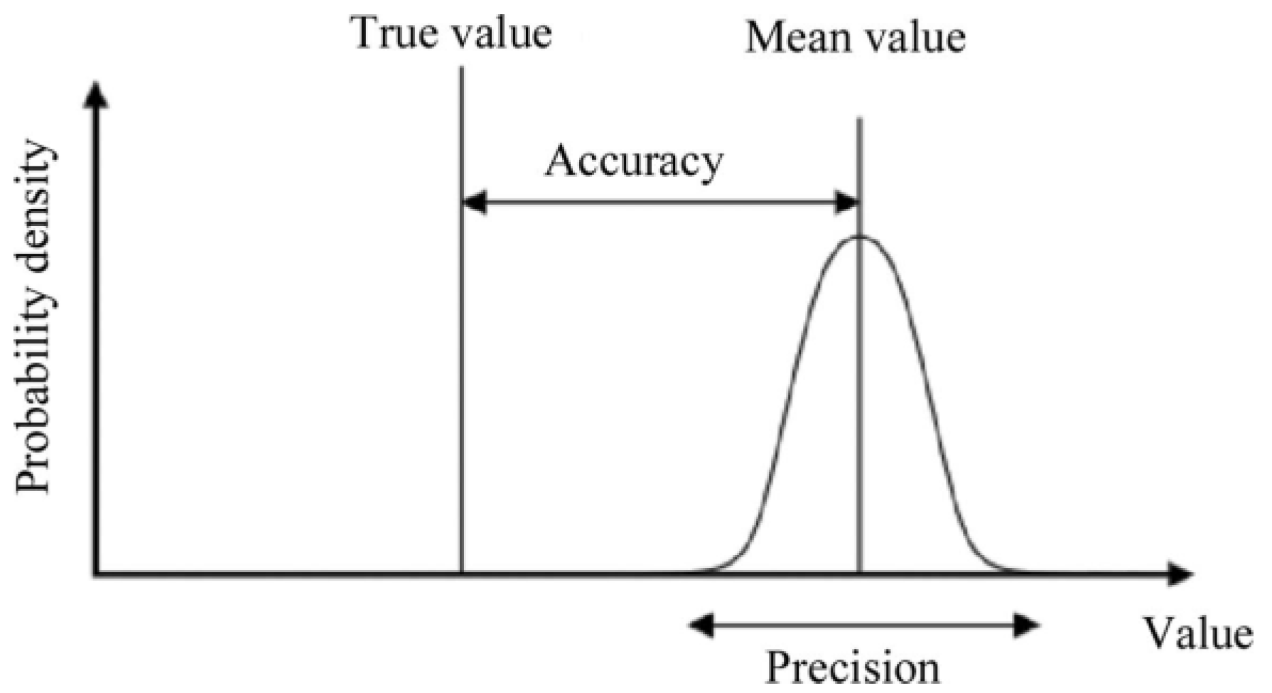
The two words for experimental uncertainties, “precision” and “accuracy”, are used with different meanings in measurement science, as shown in Figure 1 [1]. Accuracy means a bias from the true value or a systematic error, whereas precision refers to a deviation from the mean value or a random error. The present work has aimed at developing a high-“accuracy” detector system for high-“precision” X-ray total scattering measurements.
Total scattering refers to all coherent scattering such as Bragg and diffuse scattering, which originate from crystalline and amorphous materials, respectively [2]. In most materials, crystalline domains coexist with amorphous domains such as lattice defects. Therefore, Bragg and diffuse scattering should be measured on an equal basis. However, such total scattering measurements have been still challenging, even by using synchrotron X-rays. Bragg scattering, which gives rise to high and sharp peaks, has been measured with a high Q (the magnitude of scattering vector) resolution setup [3]. On the other hand, diffuse scattering, which gives rise to lower, broader peaks, has been measured with a wide Q range setup [4]. To measure both scattering simultaneously, it is necessary to meet three requirements of total scattering data collected with a single setup: the maximum Q value (Qmax) of 30 Å−1, a Q step of 10−3 Å−1, and a precision of 0.1%. Detector systems in general have a trade-off between the Qmax and Q step values. In order to solve the trade-off problem, multiple silicon microstrip modules (MYTHEN, Dectris) [5] have been assembled at BL44B2 of SPring-8, which is referred to as the overlapped high-grade intelligencer (OHGI) [6]. The arrangement of fifteen modules in a curve without gap in 2θ has made it possible to cover 150° at intervals of 0.01° in 2θ at the same time. Provided that the incident X-ray energy is set at 30 keV, it is possible to meet the two requirements for Qmax and Q step. However, it was virtually impossible to achieve a precision of 0.1% due to inaccuracy in the microstrip modules, which is caused by differences in X-ray response between microstrips (X-ray response non-uniformity: XRNU).
Here, we report on how accuracy can be improved in X-ray detectors for high-precision total scattering measurements.
2. Materials and Methods
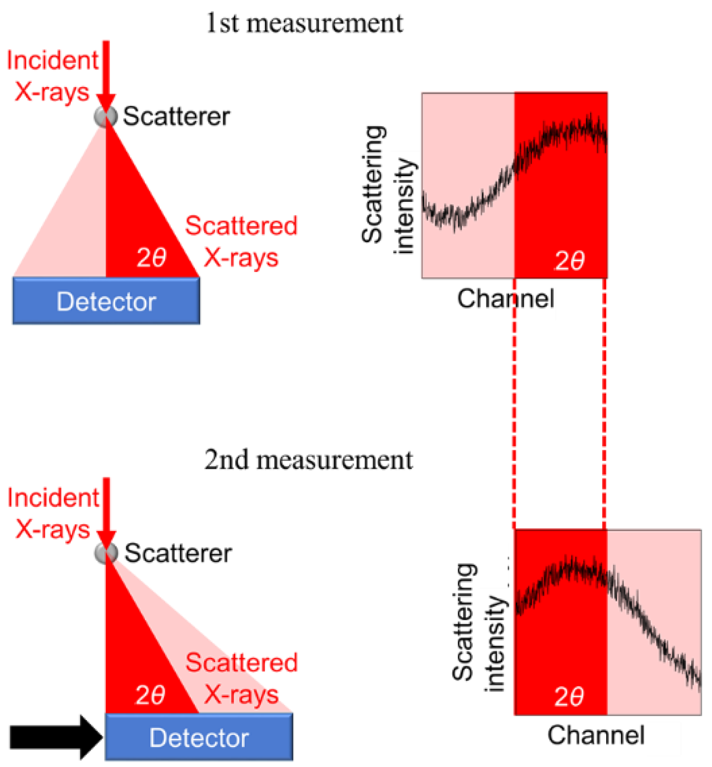
Our approach to correct scattering data for XRNU is based on the fact that XRNU appears to be a random error between microstrips [6]. Let us explain the approach using the simplest case in Figure 2. First, X-rays scattered from an object (any object can be used in principle) is measured using a detector. Next, the detector is shifted by half of its length, and then scattered X-rays are measured under the same condition. Ideally, the first scattering intensities at 2θ should be consistent with the second intensities at the same 2θ, measured with different channels within the Poisson noise. In practice, there are significant inconsistencies between the two intensities, which are caused by XRNU. Our approach takes an average between the two intensities to statistically estimate the reference intensities for the XRNU correction. From the ratio of the reference intensity to the raw intensity, the correction factor for each channel can be calculated. Accordingly, the reliability of the statistical approach is determined by the statistics of the reference intensities.
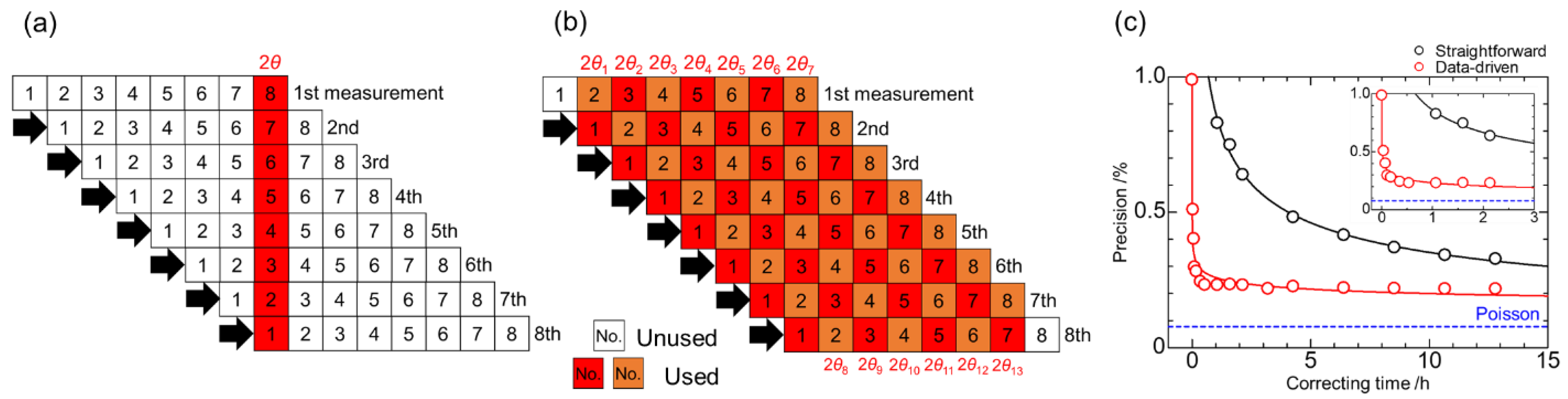
On the basis of the straightforward approach mentioned above, however, it took about half a day to achieve a precision of 0.1%. XRNU in detectors varies with experimental settings, such as X-ray energy, threshold energy, and atmospheric temperature. To overcome the time efficiency problem, the approach has been improved in terms of the algorithm for the correction factor calculations [7]. Let us explain the difference between the straightforward and improved algorithms using a one-dimensional detector with 8 microstrips in Figure 3a,b where a horizontal line corresponds to a detector. Eight scattering measurements of an object are performed, shifting the detector by one channel.
In the straightforward algorithm, only one vertical line is used to calculate the correction factor for each channel. The reference intensity, , at 2θ can be estimated as the arithmetic mean of eight intensities measured by eight channels (i = 1–8) at 2θ, as follows:
The correction factor c(i) for each channel i can be found as the ratio of the reference intensity, , to the measured intensity, , as follows:
From Figure 3a, it is found that the number of blocks used for estimating reference intensity is 8, whereas the number of those that are unused is 56.
On the other hand, in the improved algorithm, all vertical lines, except for both ends, can be used for correction factors. From each vertical line, “local” correction factors can be obtained based on the straightforward algorithm. Subsequently, multiple local correction factors for each channel are averaged using the statistical weight to obtain “global” factors. In other words, the straightforward algorithm has been improved to calculate the average of correction factors. The “local” correction factor for channel i can be estimated based on the reference intensity at 2θk in the same way as the straightforward algorithm, as follows:
The “global” correction factor, c(i), for channel i can be estimated as the weighted mean of the multiple “local” correction factors , as follows:
where is the weight for expressed by , and σk(i) is the standard deviation of . From Figure 3b, it is found that the number of blocks used for estimating reference intensity is 62, whereas the number of those which are unused is 2.
The improved algorithm has been optimized for OHGI, which has 1280 × 15 microstrips. Figure 3c shows a comparison between the two algorithms in terms of time efficiency. The straightforward and improved algorithms reach a plateau in half a day and half an hour, respectively. Moreover, the precision based on the improved algorithm is better than that based on the straightforward algorithm. For that reason, the improved algorithm has been referred to as a data-driven approach to the XRNU correction.
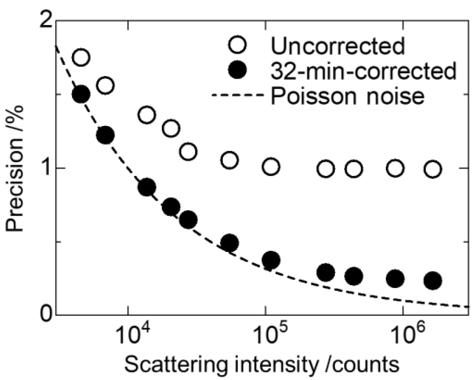
Figure 4 shows the data precision as a function of scattering intensity, which was estimated based on the standard deviation and the mean intensity from total scattering data of amorphous SiO2. In the ideal case, the precision improves with scattering intensity in accordance with the Poisson distribution. Without our correction, however, the precision reaches a plateau at about 1%, which is equivalent to a dynamic range of 104. Even though the manufacturer-supplied, flat-field correction factors were applied to the uncorrected data, the precision has not been improved. In contrast, the data-driven approach has successfully improved the precision from 1.0% to 0.1%, which is equivalent to a dynamic range of 106.
3. Results and Discussion
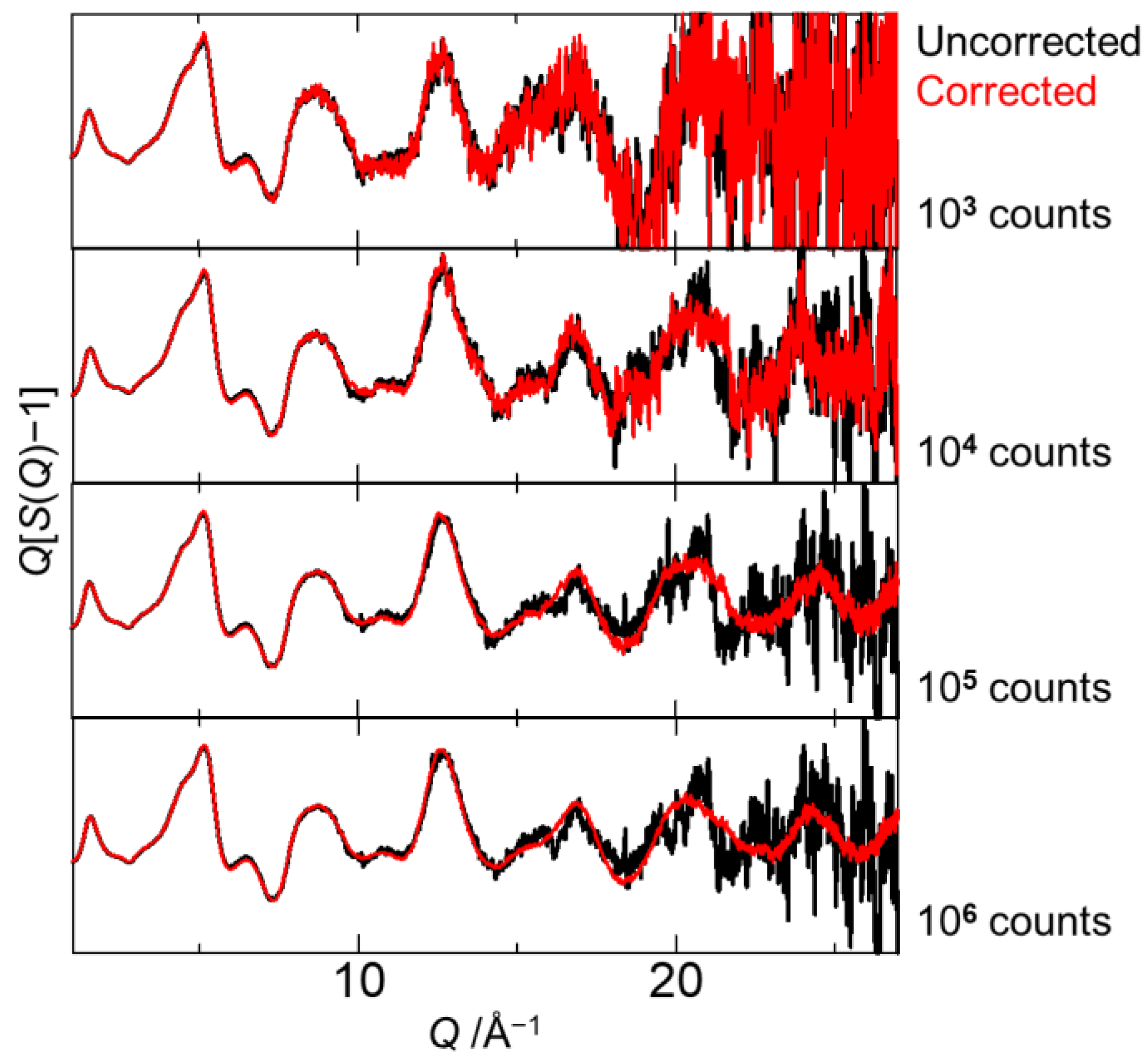
Figure 5 shows structure functions Q[S(Q)−1] of amorphous SiO2 measured with OHGI in different times, which were reduced from total scattering data with intensity from 103 to 106 counts at high Q. Without the XRNU correction, there seems to be no significant improvement in statistics at high Q even by increasing scattering intensity. In contrast, a systematic improvement in the corrected data has been observed in accordance with photon statistics. The results indicate that the XRNU correction has enabled us to observe diffuse scattering with lower and broader peaks.
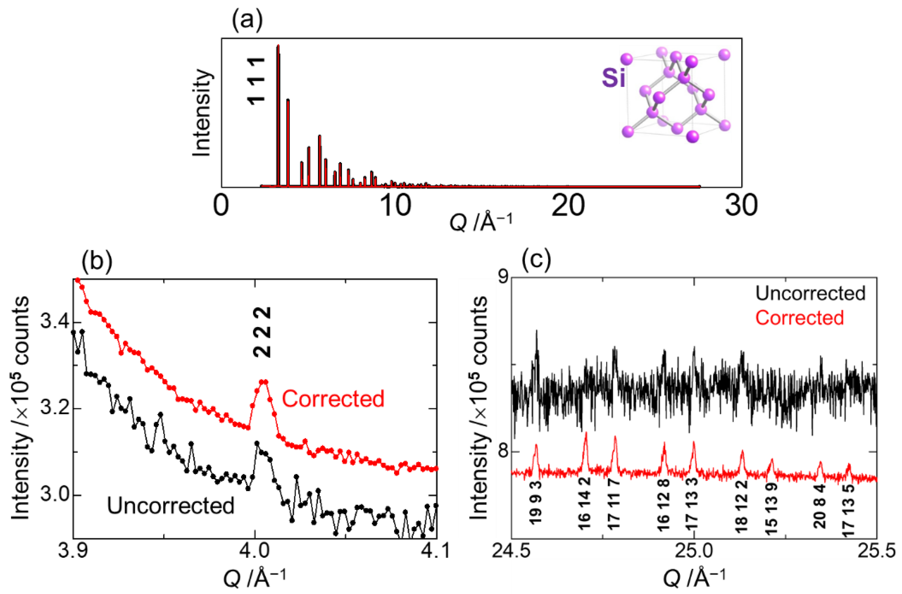
Figure 6 focuses on Bragg reflections of crystalline Si measured with OHGI. The 2 2 2 reflection from Si crystal is a forbidden reflection; nevertheless it is possible to observe the reflection due to anharmonicity of Si atoms. In fact, the reflection has been observed by using synchrotron X-ray powder diffraction [8]. However, the precision of the integrated intensity is lower than that of fundamental reflections. Figure 6b shows that the data-driven approach has considerably improved the precision. Figure 6c shows higher order reflections at high Q, which are four orders of magnitude lower than the highest reflection 1 1 1 in Figure 6a. These reflections were not observed due to the XRNU noise. The XRNU correction has successfully brought the quite weak reflections into “relief” against the background. That is why the data-driven approach has been referred to as ReLiEf (response-to-light effector) [7].
Let us discuss why the dynamic range in microstrip modules used for OHGI has been improved from 104 to 106 without the cost of Q resolution, resulting in observation of both Bragg and diffuse scattering. The specifications of the detector state a dynamic range of 107 [5]. In the strict sense, however, this value means the dynamic range not for the system but for each microstrip. In other words, the effective dynamic range has been limited by the XRNU noise. It should be emphasized that the ReLiEf method has just restored the dynamic range of the microstrip module, which enables total scattering measurements.
Atomic displacement parameters (ADP), which are estimated from Debye–Waller factors, is one of the most important parameters for structural analysis. Table 1 lists ADPs of Si obtained by different experimental techniques. Among others, inelastic neutron scattering is recognized to yield the most accurate and precise value (59.4(2) × 10−4 Å2) [9]. In the present study, the pair distribution function (PDF) analysis of total scattering data shows that the ADP is estimated to be 59.5(1) × 10−4 Å2 [10], which is agreement with the reference value within the estimated standard deviation. The results clearly indicate that our total scattering data are both accurate and precise.
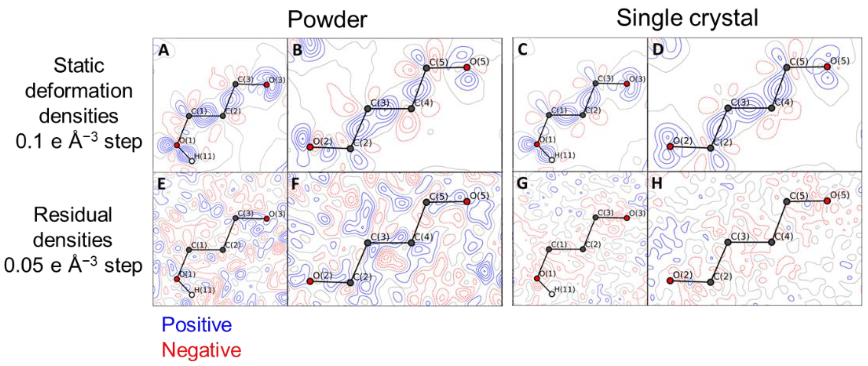
It remains challenging for powder X-ray diffraction to study valence densities of organic compounds due to lower scattering power and crystal symmetry. In fact, valence density studies have been performed using single crystals [14]. To evaluate the quality of Bragg reflections reduced from total scattering data, inorganic and organic compounds have been analyzed by the multipole refinement method [15]. Figure 7 illustrates the static deformation and the residual densities of xylitol, obtained by our powder method, which are compared to those by a reference single crystal method. The results from powders are comparable to those from single crystals. The consistency between the two results is due to the XRNU correction of the OHGI data.
4. Conclusions
In the present study, we achieved a precision of 0.1% in total scattering data by improving accuracy or XRNU in microstrip detectors, which leads to valence density studies from powders [15] and PDF studies for ADPs [10]. Consequently, the integration of hardware (OHGI) [6] into software (ReLiEf) [7] has received a positive comment, as “Nothing trumps good data” [16].
Author Contributions
Conceptualization, K.K.; methodology, K.K. and K.S.; software, K.S.; validation, K.K.; formal analysis, K.K. and K.S.; investigation, K.K. and K.S.; resources, K.K.; data curation, K.K.; writing—original draft preparation, K.K.; writing—review and editing, K.K. and K.S.; visualization, K.K.; supervision, K.K.; project administration, K.K.; funding acquisition, K.K. All authors have read and agreed to the published version of the manuscript.
Funding
This work was supported by JST, PRESTO Grant Number JPMJPR1872, Japan.
Data Availability Statement
The data presented in this study are available on request from the corresponding author.
Acknowledgments
The authors thank B. B. Iversen of Aarhus University, Demark for charge density and PDF studies. The synchrotron radiation experiments were performed at BL44B2 of SPring-8 with the approval of RIKEN.
Conflicts of Interest
The authors declare no conflict of interest.
References
- Helliwell, J.R. Combining X-rays, neutrons and electrons, and NMR, for precision and accuracy in structure–function studies. Acta Crystallogr. 2021, A77, 173–185. [Google Scholar] [CrossRef] [PubMed]
- Egami, T.; Billinge, S.J.L. Underneath the Bragg Peaks: Structural Analysis of Complex Materials, 2nd ed.; Pergamon: Oxford, UK, 2012. [Google Scholar]
- Fitch, A.N. The high resolution powder diffraction beam line at ESRF. J. Res. Natl. Inst. Stand. Technol. 2004, 109, 133–142. [Google Scholar] [CrossRef] [PubMed]
- Chupas, P.J.; Chapman, K.W.; Lee, P.L. Applications of an amorphous silicon-based area detector for high-resolution, high-sensitivity and fast time-resolved pair distribution function measurements. J. Appl. Crystallogr. 2007, 40, 463–470. [Google Scholar] [CrossRef]
- Schmitt, B.; Brönnimann, C.; Eikenberry, E.F.; Gozzo, F.; Hörmann, C.; Horisberger, R.; Patterson, B. Mythen detector system. Nucl. Instrum. Methods Phys. Res. A 2003, 501, 267–272. [Google Scholar] [CrossRef]
- Kato, K.; Tanaka, Y.; Yamauchi, M.; Ohara, K.; Hatsui, T. A statistical approach to correct X-ray response non-uniformity in microstrip detectors for high-accuracy and high-resolution total-scattering measurements. J. Synchrotron Rad. 2019, 26, 762–773. [Google Scholar] [CrossRef] [PubMed] [Green Version]
- Kato, K.; Shigeta, K. On-demand correction for X-ray response non-uniformity in microstrip detectors by a data-driven approach. J. Synchrotron Rad. 2020, 27, 1172–1179. [Google Scholar] [CrossRef] [PubMed]
- Nishibori, E.; Sunaoshi, E.; Yoshida, A.; Aoyagi, S.; Kato, K.; Takata, M.; Sakata, M. Accurate structure factors and experimental charge densities from synchrotron X-ray powder diffraction data at SPring-8. Acta Crystallogr. 2007, A63, 43–52. [Google Scholar] [CrossRef]
- Flensburg, C.; Stewart, R.F. Lattice dynamical Debye-Waller factor for silicon. Phys. Rev. B 1999, 60, 284–291. [Google Scholar] [CrossRef]
- Beyer, J.; Kato, K.; Iversen, B.B. Synchrotron total-scattering data applicable to dual-space structural analysis. IUCrJ 2021, 8, 387–394. [Google Scholar] [CrossRef] [PubMed]
- Spackman, M.A. The electron distribution in silicon. A comparison between experiment and theory. Acta Crystallogr. 1986, A42, 271–281. [Google Scholar] [CrossRef]
- Zhang, B.; Yang, J.; Jin, L.; Ye, C.; Bashir, J.; Butt, N.M.; Siddique, M.; Arshed, M.; Khan, Q.H. Temperature factor of silicon by powder neutron diffraction. Acta Crystallogr. 1990, A46, 435–437. [Google Scholar] [CrossRef]
- Ogata, Y.; Tsuda, K.; Tanaka, M. Determination of the electrostatic potential and electron density of silicon using convergent-beam electron diffraction. Acta Crystallogr. 2008, A64, 587–597. [Google Scholar] [CrossRef] [PubMed]
- Madsen, A.Ø.; Sørensen, H.O.; Flensburg, C.; Stewart, R.F.; Larsen, S. Modeling of the nuclear parameters for H atoms in X-ray charge-density studies. Acta Crystallogr. 2004, A60, 550–561. [Google Scholar] [CrossRef] [PubMed]
- Svane, B.; Tolborg, K.; Kato, K.; Iversen, B.B. Multipole electron densities and structural parameters from synchrotron powder X-ray diffraction data obtained with a MYTHEN detector system (OHGI). Acta Crystallogr. 2021, A77, 85–95. [Google Scholar] [CrossRef] [PubMed]
- Pinkerton, A.A. Nothing trumps good data. Acta Crystallogr. 2021, A77, 83–84. [Google Scholar] [CrossRef] [PubMed]
Figure 1.
The concepts of precision and accuracy in measurement science [1].
Figure 1.
The concepts of precision and accuracy in measurement science [1].

Figure 2.
Schematic drawing of a measurement process to statistically estimate reference intensities for the XRNU correction.
Figure 2.
Schematic drawing of a measurement process to statistically estimate reference intensities for the XRNU correction.

Figure 3.
Comparison between the straightforward and improved algorithms to calculate correction factors. (a) The straightforward algorithm; (b) the improved algorithm; (c) the precision as a function of correcting time, which was estimated from total scattering data of amorphous SiO2 measured with OHGI.

Figure 4.
The data precision as a function of scattering intensity, which was estimated from total scattering data of amorphous SiO2 measured with OHGI. The corrected data is based on the 32 min correction using the improved algorithm.
Figure 4.
The data precision as a function of scattering intensity, which was estimated from total scattering data of amorphous SiO2 measured with OHGI. The corrected data is based on the 32 min correction using the improved algorithm.

Figure 5.
Comparison in diffuse scattering before and after the XRNU correction. Reduced structure functions of amorphous SiO2 as a function of scattering intensity at high Q.
Figure 5.
Comparison in diffuse scattering before and after the XRNU correction. Reduced structure functions of amorphous SiO2 as a function of scattering intensity at high Q.

Figure 6.
Uncorrected and corrected total scattering data of crystalline Si. (a) The whole range in Q; (b) the forbidden reflection at low Q; (c) higher-order reflections at high Q.
Figure 6.
Uncorrected and corrected total scattering data of crystalline Si. (a) The whole range in Q; (b) the forbidden reflection at low Q; (c) higher-order reflections at high Q.

Figure 7.
Valence densities obtained by powder X-ray diffraction (present study) [15] and single-crystal X-ray diffraction [14] of xylitol. (A,B) Static deformation densities from powder; (C,D) static deformation densities from single crystal; (E,F) residual densities from powder; (G,H) residual densities from single crystal.


Table 1.
Atomic displacement parameters (ADP) U obtained by different experimental techniques.
| TS-PDF 1 | SXRD 2 | PND 3 | INS 4 | CBED 5 | |
|---|---|---|---|---|---|
| Probe | X-rays | X-rays | Neutrons | Neutrons | Electrons |
| Sample | Powder | Single crystal | Powder | Single crystal | Single crystal |
| T/K | 298 | 293–298 | 284–293 | 293 | 300 |
| U/(10−4 Å2) | 59.5(1) | 58.7(1) | 59(3) | 59.4(2) | 58.6 |
Publisher’s Note: MDPI stays neutral with regard to jurisdictional claims in published maps and institutional affiliations. |
© 2021 by the authors. Licensee MDPI, Basel, Switzerland. This article is an open access article distributed under the terms and conditions of the Creative Commons Attribution (CC BY) license (https://creativecommons.org/licenses/by/4.0/).
Share and Cite
MDPI and ACS Style
Kato, K.; Shigeta, K. High-Precision X-ray Total Scattering Measurements Using a High-Accuracy Detector System. Condens. Matter 2022, 7, 2. https://0-doi-org.brum.beds.ac.uk/10.3390/condmat7010002
AMA Style
Kato K, Shigeta K. High-Precision X-ray Total Scattering Measurements Using a High-Accuracy Detector System. Condensed Matter. 2022; 7(1):2. https://0-doi-org.brum.beds.ac.uk/10.3390/condmat7010002
Chicago/Turabian StyleKato, Kenichi, and Kazuya Shigeta. 2022. "High-Precision X-ray Total Scattering Measurements Using a High-Accuracy Detector System" Condensed Matter 7, no. 1: 2. https://0-doi-org.brum.beds.ac.uk/10.3390/condmat7010002