
Impact of Autonomous Vehicles on the Physical Infrastructure: Changes and Challenges


1
Civil Engineering Department, University of Toronto, 35 St. George, Toronto, ON M5S 1A4, Canada
2
Public Works Department, Faculty of Engineering, Cairo University, Giza 12613, Egypt
Designs 2021, 5(3), 40; https://0-doi-org.brum.beds.ac.uk/10.3390/designs5030040
Submission received: 4 June 2021
/
Revised: 2 July 2021
/
Accepted: 5 July 2021
/
Published: 8 July 2021
(This article belongs to the Section Vehicle Engineering Design)
Abstract
:Over the last few years, autonomous vehicles (AVs) have witnessed tremendous worldwide interest. Although AVs have been extensively studied in the literature regarding their benefits, implications, and public acceptance, research on the physical infrastructure requirements for autonomous vehicles is still in the infancy stage. For the road infrastructure, AVs can be very promising; however, AVs might introduce new risks and challenges. This paper investigates the impact of AVs on the physical infrastructure with the objective of revealing the infrastructure changes and challenges in the era of AVs. In AVs, the human factor, which is the major factor that influences the geometric design, will not be a concern anymore so the geometric design requirements can be relaxed. On the other hand, the decrease in the wheel wander, because of the lane-keeping system, and the increase in the lane capacity, because of the elimination of the human factor, will bring an accelerated rutting potential and will quickly deteriorate the pavement condition. Additionally, the existing structural design methods for bridges are not safe to support autonomous truck platoons. For parking lots, AVs have the potential to significantly increase the capacity of parking lots using the blocking strategy. However, the implementation of this parking strategy faces multiple issues such as the inconsistent marking system. Finally, AVs will need new infrastructure facilities such as safe harbor areas.
1. Introduction
Over the last few years, autonomous vehicles (AVs) have gained significant attention from both research and industry because of the rapid innovations in artificial intelligence technology in addition to the capabilities of the new sensing technology [1,2,3]. In general, there are five levels of automation functionality, according to the National Highway and Transportation Safety Administration. Level 0: no automation. Level 1: automation of one control function such as lane keep assist or autonomous control, level 2: automation of two control functions, level 3: limited self-driving but expect the driver to take control at any time with adequate warning, level 4: drivers are not expected to take control at any time of the trip, level 5: full self-driving with no human control [4]. Given the rapid growth in vehicle automation technology, there is a pressing need to uncover the impact of AVs on the physical infrastructure.
From the road infrastructure perspective, AVs can be very promising as it is frequently mentioned in multiple studies that AVs have the potential to increase traffic safety, reduce vehicle ownership, allow passengers to be engaged in other activities (which means that the trip time will not be considered as an economic loss), reduce the parking demand which in turn reduces congestion of vehicles searching for a parking space, reduce emissions and energy due to the platooning effect, the smooth start and stops, and the reduction in the number of engines starts due to the reduction in required fleet size, increase coverage and accessibility for aged, disabled individuals, and people with limited transportation [5,6,7,8,9,10,11,12,13,14,15,16,17,18,19,20,21,22,23,24,25,26,27,28,29,30,31,32,33]. However, AVs might introduce new risks and challenges for the current infrastructure. For instance, the change in the vehicle behavior or the driving behavior is expected to introduce new risks and deteriorate the performance of the existing network. Thus, this impact might have a significant impact on the economic and environmental costs.
As mentioned above, AVs have gained significant attention from researchers in terms of their implications, benefits, technological requirements, and public acceptance [5,6,7,8,9,10,11,12,13,14,15,16,17,18,19,20,21,22,23,24,25,26,27,28,29,30,31,32,33,34]. However, how AVs will be deployed in the future mainly depends on the level of investment from the public and private sectors in the infrastructure. Research on the physical infrastructure requirements for autonomous vehicles is still in the infancy stage that even the highways and roads planning and guidance documents followed by most transportation authorities, such as DMRB in the UK, do not take into account AVs at all [35]. Although it is expected that AVs will change both the digital and physical infrastructure, little attention has been paid to the physical infrastructure requirements and the main focus of the existing studies in the literature is on the digital infrastructure [36]. Thus, the main objective of this paper is to assess the physical infrastructure requirements to support the deployment of AVs. This paper focus on analyzing the impacts of AVs on multiple branches of the physical infrastructure as follows:
- The impact of AVs on the geometric design: in this study, the AASHTO design guidelines will be reviewed and updated to analyze the impact of deploying AVs on the stopping sight distance, passing sight distance, horizontal curve, and vertical curve design.
- The impact of AVs on the design of the parking lots.
- The impact of AVs on the pavement design.
- The impact of AVs on the structural design of bridges.
- Infrastructure requirements and new risks or challenges that will be introduced with the deployment of AVs: such as the required safe harbor areas, the need for a traffic management technique, and the required signing and marking.
2. Geometric Design
This section focuses on investigating the possible change in the geometric design elements when a fully AVs fleet navigates on the roads. In general, driving behavior is the major factor that influences the design elements [37]. For example, the driver’s reaction time, eye height, and other human-related behaviors are the major factors that influence the design of highway geometric elements. The study by McDonald highlighted that the geomatic design elements will change once the entire fleet consists of AVs without detailed analysis [38]. Thus, this section focuses on the changes in the geometric elements that will be affected by switching from traditional driving to autonomous driving such as the stopping sight distance, the decision sight distance, and the length of the vertical curve. Additionally, in this section, the current AASHTO standard will be revised and updated in order to be compatible with autonomous driving.
2.1. Stopping Sight Distance (SSD) Model
The stopping sight distance (SSD) consists of two main distances: the perception and reaction distance and the braking distance [39]. The perception and reaction distance mainly depends on the driver’s attention and response. On the other hand, the braking distance depends on the mechanical characteristics of the vehicle. In this study, the mechanical performance of the human-driven and autonomous vehicles will be assumed to be identical. Additionally, the surrounding conditions such as weather conditions, grade, and road surface condition will be assumed to be identical. As a result, the braking distance remains the same in the two cases. In a mathematical formula, the SSD can be expressed using Equation (1).
where:
- SSD = Stopping Sight Distance (m)
- V = Design Speed (km/h)
- t = Perception and reaction time (s) (Typically 2.5 s)
- a = Deceleration Rate (m/s2) (Typically 3.4 m/s2)
- G = Grade of the Road
Previous studies that focus on the reaction of AVs show that AVs can react quickly, in 0.2 s, after the detection of an obstacle [40] then the vehicle starts braking. In this study, a reaction time of 0.5 s, which is a conservative value, will be used. The difference between the SSD of AVs and human-driven vehicles is shown in Figure 1. The resulting SSDs for the human-driven vehicles and AVs, resulting from the previous equation in the case of level roads, are shown in Table 1. Figure 2 shows the SSD for different upward grades for both human-driven vehicles and AVs, while Figure 3 shows the SSD values for downgrades. The figures illustrate that AVs can significantly reduce the SSD due to their quick reaction.
2.2. Decision Sight Distance (DSD)
In general, the decision sight distance (DSD) is used to offer the drivers the safe distance that is required to make a complex maneuver or to deal with a complex situation. In other words, the DSD is used to allow the driver to detect the threat and react safely to take the correct action [41]. DSD involves multiple maneuvers starting from stopping, changing lanes, or decreasing the speed of the vehicle. The DSD is classified into five categories or five movements from A to E. Maneuvers A and B focuses on providing sufficient stopping distance on rural and urban roads and the DSD in this case is calculated using Equation (2).
where:
- DSD = Decision Sight Distance (m)
- V = Design Speed (km/h)
- t = Pre-maneuver time (s)
- a = Driver Deceleration Rate (m/s2)
The design guidelines state that avoidance maneuver A, stop on a rural road, needs a pre-maneuver time of 3 s, while avoidance maneuver B, stop on a rural road, needs a pre-maneuver time of 9.1 s [39]. The previous values are needed to offer the drivers (human drivers) the required distance to complete the maneuver safely. However, in the case of AVs, the reaction time is different from the human driver reaction time. Thus, the required distance should be shorter similar to the case of SSD. In other words, AVs will not need longer distances to react in complex situations and the reaction time for the DSD will similar to the reaction time of the SSD = 0.5 s. In this case, for maneuvers A and B, the DSD will be the same as the SSD in the case of level roads. Table 2 and Figure 4 show the difference between the DSD for maneuver A and B for human-driven vehicles and AVs.
Additionally, the remaining three DSD maneuvers (C, D, and E) offer speed, path, or direction change on rural, suburban, and urban roads. However, these three cases are more complex than the first two cases and need further analysis and will be discussed and analyzed separately in detail in a future study.
2.3. Lateral Clearance on Horizontal Curves
In horizontal curves, the line of sight is used for ensuring the availability of a safe sight distance that allows drivers to stop before hitting a stopping obstacle [42,43,44]. While there are multiple types of horizontal curves, this section focuses on circular horizontal curves that have a curve length that is higher than the SSD to show the impact of AVs on the required lateral clearance distance or on the sightline. In this case, the horizontal sightline offset (HSO) can be calculated using the formula shown in Equation (3).
where:
- R = curve radius (m)
- S = Sight distance (m) and in general this value is used as the SSD in order to let drivers stop before crashing obstacles.
It must be noted that the curve radius in the previous equation is calculated using the superelevation rate and speed. Since it is assumed that AVs are similar to human-driven vehicles except for the driving behavior, it can be stated that the required minimum curve radius will be the same in both cases: human-driven and autonomous vehicles. Thus, the required SSD for AVs is much lower than human-driven vehicles, and in turn, the required safe HSO distance will be lower for AVs. Figure 5 shows the required design controls for achieving the safe stopping sight distance for different speeds (60, 80, 100, and 120 km/h) on Horizontal Curves for human driving and AVs. Figure 6 shows the difference in the required safe values of HSO distances in the two cases: human-driven vehicles in blue and AVs in red.
2.4. Length of Vertical Curve
2.4.1. Length of Crest Curve
According to the AASHTO’s standards, the length of the crest curve is calculated using one of the two formulas shown in Equations (4) and (5).
where:
- L = Length of the vertical curve, m
- S = Sight distance, m
- h1 = Height of eye above roadway surface, m (typically = 1.08 m)
- h2 = Height of object above roadway surface, m (typically = 0.6 m)
- A = (in percent) is the algebraic difference in grade.
The main difference between AVs and human-driven vehicles in the previous models is the SSD and the eye height (h1). The eye height in the case of the AVs will depend on the LiDAR sensor instead of the driver’s eye. The study by Garcia et al. [45] concluded that the location of the LiDAR sensor in the vehicle affects the sight distance. Thus, the sight distance increase with the increase in the height of the sensor. Thus, the location of the sensor is a critical factor for estimating the required curve length. As a result, in this study the height of the LiDAR sensor will replace the driver’s eye height. In general, the sensor is added on top of the vehicle, which offers a higher (h1) value. As stated in the study by Khoury et al. [37], Google self-driving project tested their AV technology on the Toyota Prius and Lexus RX450h [46] which have heights of 1.47 m and 1.685 m. Waymo produces its own AVs that have a height of 1.555 m and the height of the LiDAR is 0.284 m [47]. For google self-driving cars, the LiDAR sensor was supported in a 0.3 m support that increases the (h1) value. In this case, the height of the sensor = 1.47 + 0.3 + 0.284 = 2.054 m. For the Waymo vehicles, there is no sensor support used so the height of the sensor = 1.555 + 0.284 = 1.84 m. Thus, the lower height is the critical one as it results in a higher curve length. Thus, in this study, h1 of 1.84 will be used. Using this assumed value, the resulting curve lengths, calculated using the equations, for both human-driven vehicles and AVs are shown in Table 3. Table 4 summarizes the required K-value (rate of curvature) for different design speeds. The K value is defined as the required curve length for 1% change in the grade and in general, the length of the curve, is calculated using Equation (6).
where:
- L = crest curve length
- K = Rate of vertical curvature
Figure 7 shows the required crest curve length for different algebraic differences in grade at different speeds for the two cases AVs and human-driven vehicles. The solid lines represent the case of AVs and the dashed lines represent the case of human-driven vehicle. In order to visualize the difference between the two cases, the logarithmic scale was used in the Y-direction. It can be seen that the required safe curve length is much lower in the case of AVs than human-driven vehicles.
2.4.2. Length of the Sage Curve Length
According to the AASHTO’s standards, the length of the crest curve is calculated using one of the two formulas shown in Equations (7) and (8).
where:
- L = Length of the vertical curve, m
- S = Sight distance, m
- H = Headlight height, m
- β = Divergence of the light beam from the longitudinal axis of the vehicle
In general, the design of the sag curve focuses on the night vision which mainly depends on the characteristics of the headlights in terms of the height of the headlight and the inclined angle of the headlight beam. In the case of AVs, the LiDAR will be the replacement of the headlight and will be the sensor that provides visibility for the vehicle during night [48]. As discussed in the previous section the height of the LiDAR sensor will be taken as 1.84 m replacing the traditional headlight height in traditional vehicles which is 0.6 m. Similarly, the inclined angle of the headlight beam will replace the traditional inclined angle of the headlight beam. The manufacturers of the LiDAR sensor state that the field view of the sensor is 26.8 degrees [47]. However, it must be mentioned that this angle is for one manufacturer and in the future multiple manufacturers will be working on the production of LiDAR sensors. As a result, a conservative value should be used in this case similar to the value used in the study by Khoury et al. [37] as they assumed that the inclined angle of the headlight beam is 13.4 degrees and this value is the value used in this study. Using this assumed value, the resulting curve lengths, calculated using the equations, for both human-driven vehicles and AVs are shown in Table 5. Table 6 summarizes the required K-value (rate of curvature) for different design speeds. It can be seen that there is a significant difference between the required sag curve length for AVs and the required sag curve length for human driving behavior. This difference comes from the reduction in the SSD and the increase in the inclined angle of the headlight beam in the case of fully AVs. Figure 8 shows the required sag curve length for different algebraic differences in grade at different speeds for the two cases AVs and human-driven vehicles. The solid lines represent the case of AVs and the dashed lines represent the case of human-driven vehicles. In order to visualize the difference between the two cases, the logarithmic scale was used in the Y-direction. It can be seen that the required safe curve length is much lower for the case of AVs than human-driven vehicles.
Comparing the current design criteria and the updated criterion for AVs, results show significant improvement in terms of both economic and environmental savings because of the elimination of the human factor. For example, the decrease in the required lengths of both the crest and sag curves will result in a significant reduction in the amount of fill and cut required for the construction process. This reduction means a faster and cheaper process given constant productivity rates. Additionally, in the case of borrowing fill material, less material will be required and thus less construction cost.
2.5. Lane Width
It has been frequently mentioned in the literature that the standards regarding the lane width can be reduced when all vehicles become automated and connected because of the lane-keeping system [49]. Thus, additional lanes can be created and dedicated for other purposes such as platooning lanes [50,51]. It is mentioned in multiple studies in the literature that the high communication between AVs will make it possible to minimize the lane width to reach 2.4 m (8 ft) as shown in Table 7.
2.6. Horizontal Curve Design
The main factors that influence the curve radius are the superelevation and the coefficient of side friction between the tire and the pavement as shown in Equation (9).
where:
- e = superelevation rate
- fs = coefficient of side friction
- R = Curve radius (m)
- V = Design speed (km/h)
The coefficient of side friction depends on the design speed. Thus, the curve radius does not depend on the characteristics of the drivers such as the reaction time, but depends on the driving dynamics. As such, AVs will not change the required curve radius and the minimum curve radius in the case of human-driven vehicles will be the same as the required minimum curve radius in the case of AVs.
2.7. Spiral Curve Design
In general, Euler spiral, which is called “clothoid”, is used for the design of transition curves. In this spiral, the radius changes from infinity at the end of the tangent segment to the curve radius gradually at the beginning of the curve. In 1909, Shortt [59] developed the formula used for estimating the spiral length for the gradual attainment of latera acceleration on railroad track curves as shown in Equation (10). This formula is adopted by most highway agencies for the estimation of the minimum spiral length, and it is the formula used by the AASHTO for the estimation of the spiral length.
where:
- L = minimum length of spiral, m
- V = speed, km/h
- R = curve radius, m
- C = rate of increase of lateral acceleration, m/s3
In general, the rate of increase of lateral acceleration (C) is an empirical value representing the comfort and safety levels provided by the spiral curve. For railway, a value of 0.3 m/s3 is used for the C value; however, for highways, a C value between 0.3 to 0.9 m/s3 is used by most highway agencies. Thus, the main factors that influence the spiral curve design are the curve radius (does not depend on the drivers), design speed and the rate of increase of lateral acceleration that focuses on the comfort levels.
Thus, the spiral curve design does not depend on the characteristics of the drivers such as the reaction time but depends on the driving dynamics. As such, AVs will not change the spiral curve design.
2.8. Maximum Length of Straight Segments on Horizontal Alignments
Generally, roads consist of straight sections and curves. Long straight sections introduce risks as they can easily make drivers feel bored, tired or fall asleep. This issue causes the drivers either to speed up and break the speed limits or fall asleep and lose control of the vehicle, which can easily lead to the occurrence of traffic accidents [60]. As a result, when a straight line is used, it must not be too long. Thus, previous studies show that, at speeds higher than 60 km/h, the maximum straight-line length should not allow the vehicle to travel more than 70 s on the design speed, which is equivalent to ‘20 × V’ (design speed) [61]. Thus, the human driver is the main factor for adding the limitation on the maximum straight sections. In AVs, the human factor will not be a concerning factor anymore. Thus, the limitation of the maximum straight section length can be relaxed, and the maximum length of straight sections will not be restricted in the ear of AVs.
3. Parking
Research studies on the parking of AVs show that AVs can significantly reduce the number of the required parking lots, especially in the context of shared AVs as vehicles will be serving customers at different times, which reduces the number of required parking spots [62,63,64,65]. Additionally, the autonomous valet parking system will allow vehicles to park closer to each other and thus the parking lots will be able to serve more vehicles. This provides new opportunities for both the users and the infrastructure provider as the user will not have to search for a space to park and increase the number of vehicles using the parking area doe parking owners. Theoretical speaking, AVs will be able to park without the need for the door space, which could enable 20% more free spaces. Furthermore, AVs can block each other and let each other out when necessary. A study by Audi shows that a parking lot for AVs can take 2.5 times the conventional vehicles [66]. Figure 9 shows a comparison between the parking layout and spaces for the same parking in the case of conventional vehicles and AVs using the proposed blocking technique [67,68]. On the other hand, this method faces two main problems. Firstly, this method requires remote control of the vehicle by the parking operator which might expose the vehicle to cyber-security threats also safeguards might be required if the vehicle does not respond. Secondly, this method will need an electronic payment method as no occupant will be in the vehicle.
A major issue in the current parking lots is that most of them are privately owned and do not have a consistent marking system so the AVs will struggle in such an environment. As a result, it is essential to agree on international standards for AVs parking. To achieve the highest level of advantages of AVs, parking might be designed for AVs only with the required marking and sign with no pedestrians or human-driven vehicles. In the early years, companies that own a fleet of AVs might benefit from the blocking parking strategy and increase the land use value. Additionally, parking lots of AVs will require drop-off and pick-up areas to allow people to call or drop off their cars. This area may be small at the beginning and expanded with the increase in the use of the AVs.
Finally, the current parking lots do not support AVs safe operations as most of the current parks are underground parks where the GPS signals are lost or weak, which causes confusion for AVs. One suggested solution is the use of Bluetooth and near field communications to support the navigation of the vehicles in the parking lot [69]. Whereas there is no clear plan in any country on when or how these parking lots will be retrofitted.
4. Pavement Performance and Life Cycle
AVs are more likely to operate with high accuracy in the middle of the lane using the lane-keeping system [70,71]. Thus, AVs will have a significant influence on the pavement condition and will accelerate the appearance of rutting, cracking, and other deteriorations [72]. As a result, some areas beneath the wheels need to be strengthened using higher stiffness and more deformation resistance materials, especially, in the case of using dedicated AVs lanes [73]. In general, flexible pavement consists of a surface pavement layer in direct contact with the running traffic followed by aggregate layers on top of the soil (base, subbase, and subgrade). The asphalt pavement surface layer consists of hot mix asphalt and the thickness of this layer is estimated based on the traffic loading, life cycle, and the properties of the asphalt mix components [74].
One of the major distresses of the flexible pavement is rutting [75,76] and this became a concerning issue for highway engineers because of the developments in truck loads and the associated increase in the wheel load and tire pressures on the pavement, which increase the severity of this issue [77]. Rutting can be defined as the permanent deformation that appears on the pavement surface on the wheel path referring to accumulation in the irrecoverable strains from repeated load cycles. Rutting can be hazardous as it might cause sliding of vehicles and drivers might lose control of their vehicles. In general, there are two types of rutting: subgrade rutting which is caused by the lateral movement of the lower layers (base, subbase, and subgrade) and asphalt mix rutting which is caused by the vertical movement of the lateral creep in the wearing course layer [78]. Multiple factors affect the pavement performance and rutting resistance such as the properties of the material, climate conditions, traffic intensity, and speed. In the future, when AVs are on the roads, capacity of roads, traffic speed, and wheel wander will change and affect the pavement rutting performance. The study by Chen, Balieu, and Kringos [79] provides a detailed analysis of the impact of AVs on the performance of the asphalt pavement as follows:
- Wheel wander: the lane-keeping system or the steering control of AVs will be much more accurate than traditional cars (human-driven) so the lateral wander or deviation of the wheels in the transverse direction will be reduced. The previous action will deteriorate the pavement quickly and increase the rutting potential. Chen, Balieu, and Kringos [79] used a typical pavement section in their study, which consists of asphalt course, a base layer, and a subbase layer on top of the subgrade layer. Then, a typical heavy vehicle which is equivalent to a 100-KN single axle load with a tire pressure of 750 kPa was used. For the dual tire loading, the individual tires were superimposed using the Hua and White method [80] as shown in Figure 10. To assess the impact of AVs on the pavement rutting, a parametric study was performed by specifying a wander distance of 0.26 m for normal vehicles and 0.20 m, 0.10 m, 0.05 m, and 0 m for AVs were tested after 5 × 10⁵ passes of the standard truck at a speed of 100 km/h, then the loading time was calculated and illustrated in Figure 11. It must be mentioned that the summation of the total loading time should be the same in all cases as the number of passes is fixed. The loading times calculated in the previous step were used to calculate the rutting performance of the pavement using finite elements. The maximum rut depth was calculated for different levels of wander distance and results show that the maximum rut depth jumps from 0.43 mm for a wander distance of 0.26 m (the case of human driving) to 1.19 mm for a wander distance of 0 (the case of autonomous driving) which represent 175% increase in the rut depth. As a result, it can be stated that the accuracy of AVs might have the potential to significantly accelerate the pavement rutting when compared with traditional vehicles.
- Capacity: AVs will be able to operate safely with smaller safe travelling distances than human-driven vehicles, which can increase the capacity of the roads, and in turn, will have a significant influence on the pavement performance and rutting resistance. In general, road capacity can be defined as the maximum hourly flow rate that can pass a certain point [81] and the lane capacity is defined as the multiplication of the number of vehicles present in a unit length by the average speed as shown in Equation (11).
where:
- ○
- C = capacity
- ○
- Vi = average speed
- ○
- d = traffic density per km
The lane capacity is determined by two main factors: the driver’s behavior and the mechanical properties of the vehicle such as the acceleration and deceleration and it can be expressed in a different format [82] as shown in Equation (12).
where:
- ○
- l = vehicle length
- ○
- a = acceleration rate
- ○
- t = driver reaction time.
In the case of AVs, the reaction time will be significantly reduced and thus the capacity of the road increases. In fact, it was estimated by multiple studies that AVs will significantly increase the vehicle capacity as estimated by Tientrakool et al. study that shows that the road capacity will increase by 3.2 times in the case of AVs than human-driven vehicles [83]. Additionally, the study by Shladover et al. shows that the use of cooperative adaptive cruise control will increase the capacities of roads by 80% [84]. The increase in the capacity will have a significant influence on the pavement rutting performance. The study by Chen, Balieu, and Kringos [79] shows that keeping traffic speed unchanged and increasing the capacity by 100% increases the rut depth by 40%.
- Speed: higher traffic speed means lower loading time and less impact on the pavement. In the study by Chen, Balieu, and Kringos [79], it was speculated that AVs have the potential to reduce traffic congestion as AVs will allow for the use of automatic vehicle routing that can be controlled to optimize the network performance. Additionally, AVs will operate with more safety levels than human-driven vehicles which reduces the number of traffic accidents, as 25% congestion is caused by traffic accidents [85], and improve the traffic performance, speed and reduce delays. Chen, Balieu, and Kringos [79] studied the influence of different traffic speeds for the same lane without considering the wheel wander. Figure 12 shows the maximum rut depth for different traffic speeds after ‘2 × 10⁵’ passes. Results show that pavement rutting depth decreases with the increase in traffic speed. For example, the rut depth decreases by 50% when traffic speed increases from 10 km/h to 50 km/h.
Figure 12.
Maximum rut depths with different traffic speed.

However, recent studies suggest that AVs might not reduce traffic congestion but increase congestion because AVs will motivate people to make longer trips, travel further, and make additional trips which in turn increase the VKT. Additionally, AVs might increase the VKT because of the vehicle relocation strategy searching for cheap parking lots during the low demand periods [11,17].
It can be concluded that AVs will introduce new issues for the current pavement design procedures as AVs will be able to increase the lane capacity and decrease the wheel wander. Thus, AVs have the potential to increase the pavement rutting and deteriorate the current pavement performance. On the other hand, there is a debate on the impact of AVs on the congestion level. Thus, the impact of AVs on travel speed remains unknown and will depend on the changes in public behavior in the future.
One of the proposed solutions to mitigate the impact of AVs on the pavement performance is to program the vehicles to navigate more evenly across the whole width of the lane. For example, the study by Chen, et al. (2019) [86] estimated the impact of AVs on the performance of pavement using finite elements. This study focuses on testing three different later control modes on managing AVs lateral distribution: zero-wander mode, uniform lateral distribution mode, and double-peak gaussian distribution mode. Results show that AVs can be beneficial and will increase the fatigue life of pavement if the vehicles are controlled properly in the lateral direction. Results show that the unform and double peak gaussian distribution cause up to 35% reduction in the fatigue damage and increase the pavement life cycle by up to 2.4 years. On the other hand, the zero-wander mode shows 1.56 years reduction in the life cycle of the pavement. Thus, the proper control of the vehicle can increase the life cycle of the pavement. Similarly, the study by Song, et al. (2021) [87] evaluated the impact of autonomous trucks on the fatigue damage of pavement using finite elements. This study focuses on estimating the impact of autonomous truck platoons on the pavement under different later offset between the leading and the following trucks in the platoon. Results show that increasing the lateral offset reduces the fatigue damage and increases the pavement life cycle. The study by Georgouli et al. (2021) [88] studied the impact of AVs on the pavement by reviewing the literature. Results of this study show that if AVs followed the zero-wander model, they would increase the pavement damage and reduce the pavement life cycle as shown if Figure 13. On the other hand, the distribution of the wheel wanger in an optimal way, that depends on the pavement thickness and pavement properties, can increase the pavement life cycle. Another study by Chen, et al. (2021) [89] for evaluating the impact of AVs on the pavement life and performance shows similar results. Results show that AVs with lateral distribution can be beneficial for asphalt pavement. For example, results show that AVs with lateral offset can reduce the fatigue damage by 28%. The two studies by Zhou et al. (2019) [90] and Zhou et al. (2019) [91] focus on studying the impact of different wheel wanders on the pavement performance using the Texas Mechanistic-Empirical Flexible Pavement Design System (TxME). Results show that if AVs are traveling with narrower wheel wander (compared with conventional vehicles), the rutting depth will increase by 30% and the pavement life cycle will decrease by 22%. On the other hand, the use of wider wheel wander with uniformly distributed traffic loads can be beneficial and reduce the rutting depth by 24% and increase the pavement life cycle by 16%.
However, following this programming approach means that the lane width cannot be reduced [92] so it is a cost to benefit analysis. Further research is required to analyze and compare the benefit to cost ratios of the two cases: the case of narrow lanes with high rut depth, and the case of traditional lanes with AVs that navigate evenly across the whole width of the lane that results in better pavement condition.
Additionally, In the future, the objectives and functionality of roads will change from just serving mobility to enable new functionalities such as vehicle charging, and navigation. For example, magnets have been embedded on the road in order to improve the navigation and positioning of the AVs [93]. Additionally, on-road charging or energy harvesting pavements have been suggested and studied in multiple studies in the literature [94,95,96,97,98]. Thus, the integration of these new technologies might have the potential to offer more advanced road structures and materials which are not feasible nowadays because of the cost to benefit relationship. Consequently, this integration might be promising and advantageous for the pavement construction. However, this integration will be challenging and requires further research given that all roads constructed and maintained today are built with ordinary roads.
5. Impact of Truck Platooning on Bridges
Over the last few years, platooning gained large attention from researchers and from the industry. Vehicle automation is the main technology that can be used for facilitating the formulation of platoons. Vehicle platooning provides a large number of benefits such as the reduction in the emissions and the reduction in the fuel consumption.
On the other hand, it is expected that platoons will violate the current procedures and guidelines for the structural design of bridges [99]. The main focus here is on truck platoons, not passenger vehicle platoons, as trucks are the critical or heavy vehicles used in the design of bridges. For example, the study by Yarnold and Weidner [100] investigated the impact of platooning on the current design procedure with more focus on the impact of the following parameters: bridge span, span length, bridge configuration, and the number of trucks in the platoon. Results show that the AASHTO standard specifications for Highway and Bridge are not safe to handle truck platoons in most of the case. The study by Tohme and Yarnold [101] focuses on investigating the impact of the number of trucks in the platoon and the distance on three exiting design methods: the Allowable Stress Design (ASD) method, the Load Factor Design (LFD) method, and the Load and Resistance Factor Design (LRFD) method. Results show that the existing design methods are not appropriate to deal with truck platoons. In other words, these design guidelines are not safe if truck platoons will use the bridges. Additionally, results show that the number of trucks per platoon and the spacing between trucks in the platoon are major factors that affect the internal forces in the structure of the bridge. Thus, these old structures and the current design guidelines might become a restriction for the formulation of the platoon so further research is required to develop new standards that are able to deal with platoons. The study by Kamranian (2019) evaluated the ability of the Hay River Bridge on handling truck platoons. This study investigated the impact of different truck platoon sizes: two trucks, three trucks and four trucks. Results show that the bridge has adequate capacity for a platoon of two trucks. However, larger platoon sizes are unsafe and will cause failures [102].
Two of the most comprehensive studies that analyzed the impact of different platoon characteristics on bridges are the studies by Birgisson, et al. (2020) [103] and Pillay (2020) [104] in the Texas A&M Transportation Institute (2020). This study analyzed the performance of all bridges in the state of Texas under platooning using the National Bridge Inventory (NBI) database. This study focuses on analyzing the existing conditions and how bridges that are designed using different design methods (Allowable Stress Design (ASD) method, the Load Factor Design (LFD) method, and the Load and Resistance Factor Design (LRFD)), and construction material (concrete or steel) will perform under platooning. Additionally, the impact of the number of trucks in the platoon, truck type, and truck spacing on different bridges is conducted. Finally, the study offers a prioritization scheme for prioritizing bridges according to their conditions based on the bridge capacity and truck loads. Results show that the spacing between the truck is the most important factor that affects the performance of the bridge. For example, the results show 33% increase in the number of bridges in the high priority zone when the truck spacing is increased from 30 ft to 40 ft as shown in Figure 14 that shows the number of bridges with high priority for different truck types for the case of 30 ft truck spacing and 40 ft truck spacing.
Similarly, the study by Thulaseedharan et al. (2020) [105] investigated the impact of truck platooning on 3000 bridges with different characteristics and prioritized these bridges using the same methodology mentioned in the previous two studies. This study shows that the number of trucks in the platoon has a minor impact on the number of bridges with high priority. For example, results show 7% increase in the number of bridges within the high priority zone when the platoon size increases from two trucks to three trucks. On the other hand, results show that the spacing between the trucks is the major factor that affects the performance of the bridges. For example, this study shows 68% increase in the number of bridges in the high priority zone when the truck spacing is reduced from 9 m to 12 m as shown in Figure 15. Thus, controlling the impact of the platoons on the bridges can be done by controlling the spacing between the trucks within the platoon.
As mentioned in all previous studies, the spacing between the trucks in the platoon is the major factor that significantly affects the safety of bridges. Thus, restricting the spacing between trucks in the platoons might be the solution for controlling or limiting the impact of truck platoons on the existing bridges. For newly constructed bridges, they must take into account truck platoon and new standards for the design of bridges must be developed in order to prepare for the future.
6. Emergency Refugee Areas
In the future, when AVs will operate on the roads, passengers will be able to participate in other activities. However, this introduces new issues and risks in case of vehicle malfunctioning or deterioration in the surrounding environment. This case might need some human interaction and ask the passengers to take control of the vehicle, but it is possible that the driver is not ready to take control of the vehicle so AVs will need a safe area to use until the driver takes control. In general, the hard shoulder area is used along the road but most of these areas are converted into travelling lanes. On the other hand, sometimes emergency refuge areas (ERA) which are located at specified intervals, such as 2.5 km in the UK, and have specific length, such as 100 m long. However, there are many concerns about these areas as many accidents took place within proximity of these areas, making these places unsafe for AVs [68]. As a result, the use of emergency areas is important for AVs to offer the vehicles a safe area in case the AV cannot operate safely in the current surrounding environment or in case of any malfunctioning [106]. The locations of these areas must be mapped and documented so that AVs can plan to stop if the occupant does not take control. These emergency areas should be located at specified intervals in areas where the environment is not severe in order to help the vehicle to stop safely in case of malfunctioning. For example, Arizona is one of the cities that take the lead in AVs testing because of the favorable conditions such as good weather and flat land [107]. Consequently, the need for emergency areas will be reduced in the case of AVs malfunctioning. On the other hand, in case of extreme environmental conditions, the need for the emergency areas might become very expensive as the surrounding conditions increase the need for the emergency areas. In this scenario, AVs will need these areas to stop in case the vehicle cannot operate in the surrounding environment or in case of vehicle malfunctioning. Two main solutions might help in providing the emergency areas:
- Converting the on-street parking spaces into emergency areas as it is mentioned in a large number of studies that AVs will significantly reduce the parking demand up to 90%. Additionally, AVs will be able to search for the nearest parking lots; thus, AVs will not rely on the on-street parking, which will free up spaces on the roads [26,27,28,91]. Thus, the on-street parking spaces can be converted into AVs emergency areas.
- The reduction in the distance between vehicles can make the roads narrower and thus the remaining spaces can be used as AVs emergency areas.
The standards for these emergency areas require further research in order to specify the required area dimensions (length and width). Additionally, the standard regarding the safe intervals for constructing these areas requires further research.
7. Traffic Management
AVs are expected to depend on accurate road mapping to complete their journey safely [108]. However, traffic incidents are stochastic events that change the road layout and AVs must be able to navigate safely in all cases. Additionally, roadway maintenance work is expected, which results in changing the road layout and the locations where the vehicles are expected to travel. As a result, depending on accurate mapping might not be enough as lane closures, and traffic incidences might add new risks [109]. Currently, there are multiple websites that provide accurate information regarding traffic incidents, such as waze.com in the UK. However, this information only contains details reading the incidence cause and time without accurate information on the incidents’ on-site conditions, which makes it hard for AVs to navigate safely [62]. Thus, these changes in the surrounding environment might require additional safety measures such as:
- The use of geo-location cones, barriers on the site, or setting a virtual geofence that can be detected by AVs.
- The use of V2I technology that facilitates the digital roadside communication that provides AVs with real-time data and information regarding the status of the road ahead [73].
8. Traffic Signs and Marking
AVs need highly visible curves, speed limits, and other signage in order to safely complete the tasks of driving, navigation, and parking [73,110,111]. However, the current marking and signing technique does not support AVs navigation. For example, in North America, the faded road markings represent a major issue for the safe navigation of AVs [112]. Additionally, in Europe, the nonstandard road signs represent a major issue that causes confusion for AVs and it is also cited as a major issue that faces the current road users or, in other words, drivers [113]. Recently, the use of hydro-plastic led to a phenomenon called ghost marking which is a source of confusion for AVs [92]. In fact, both Tesla and Volvo complained about the poor quality of the existing marking and stated that these markings confuse their cars [62,114].
Additionally, the variation in the road signage is the second challenge facing AVs, so coding is the main principle for sending information in a recognizable and standardized way. Standard color, shape, font, line spacing, and luminance contrast are major factors that should be considered even for human drivers [115]. However, the historical standards for coding have changed but outdated signs remain on the road network. Thus, this variety in the signage standards introduces new challenges for AVs navigation. In general, there are many factors that impact the process of detection and recognition of the signs for AVs such as [62,68]:
- Inconsistent signs: the lack of consistency in the application of signs, and sign location can be problematic and causes uncertainty on how the vehicle will react in these conditions.
- Obscured signage: in many scenarios, signs might be Obscured partially or fully because of many factors such as other vehicles, vegetation, and the existing roadside infrastructure. This issue requires research in order to ensure the adequate detection of the signs in all conditions.
- Varying illumination: many factors might affect the visibility of AVs such as the weather conditions, the low lighting conditions, and low sun angle. Additionally, the degraded retroreflective material will affect the visibility of AVs during the night.
- Lack of signage.
The development and the new V2I communication technologies might become the key solution for the marking and signage issues. One of the main examples of the potential V2I benefit is the new smart signs and marking provided by 3M, which is a leading firm in the US with products related to traffic signage printing and production and marking [115]. These signs and marking provide AVs with the required digital information in order to improve the navigation and safety of the vehicle. The marking used is a new magnet pavement lane marking that is durable, removable, and easy for AVs to detect even in extreme weather conditions. Additionally, the signs, which are compatible with the traditional signs, are retroreflective signs that enhance readability, which could enable accurate navigation and faster decision-making for both drivers and automated vehicle systems. On the other hand, one of the main advantages of using AVs is that AVs sensors might be used for reporting any signs or marking defects to the responsible authorities [73].
9. Conclusions and Recommendations for Further Research
Over the last few years, AVs gained significant attention from both research and industry because of the rapid innovations in the artificial intelligence technology in addition to the new sensor technology capability. AVs have gained significant attention from researchers in terms of AVs implications, benefits, technological requirements, and public acceptance. However, research on the physical infrastructure requirements for autonomous vehicles is still in the infancy stage. Thus, this paper investigates the impact of AVs on the physical infrastructure with the objective of revealing the infrastructure changes and challenges in the era of AVs.
9.1. Geometric Design
The behavior of the drivers is the main factor that influences the SSD and DSD. In AVs, the vehicle will be able to react faster than a human driver and thus AVs will have substantially lower SSD and DSD. The SSD is the main factor that influences the lateral clearance on horizontal curves. Thus, AVs can substantially reduce the required lateral clearance. Furthermore, the drivers’ characteristics such as the eye height and reaction time are the main factors that affect the required vertical curve length. Thus, AVs can significantly reduce the required curve length. Finally, AVs have the potential to reduce the required lane width to a width of 2.4 m (8 ft). On the other hand, some of the geometric elements will not change in the era of AVs. For example, the required curve radius and spiral curve length will be similar for both human-driven vehicles and AVs as these elements do not depend on the characteristics of the human drivers but depend on the driving dynamics. Thus, overall speaking, the results show that AVs could substantially lower the requirements of geometric design. Comparing the current design criteria and the updated criterion for AVs, results show significant improvement in terms of both economic and environmental savings because of the elimination of the human factor. For example, the decrease in the required lengths of both the crest and sag curves will result in a significant reduction in the amount of fill and cut required for the construction process. This reduction means a faster and cheaper process given constant productivity rates. Additionally, in the case of borrowing fill material, less material will be required and thus less construction cost. Thus, with a fleet of fully autonomous vehicles, the suggested changes result in cheaper road designs with a reduced environmental footprint. On the other hand, further research is required to investigate the potential changes in the physical infrastructure when a mixed traffic of AVs and human-driven vehicles are sharing the roads with different levels of AVs market penetration. AVs offer shorter reaction times and distances; however, the impact of AVs on the transition period is unknown. As a result, further studies are required to estimate the desired geometric configurations, such as the length of the acceleration and deceleration lanes and the desired weaving section length in the transition period. No doubt that the human factor will dominate in this transition period; however, the requirements might be increased or become more conservative as human drivers will not be familiar with interacting with AVs. Thus, the use of more conservative values might be desired for safety and comfort reasons.
9.2. Pavement Design
In the future when AVs are on the roads, the capacity of roads, traffic speed, and wheel wander will change and affect the pavement performance. The decrease in the wheel wander and the increase in the lane capacity will bring an accelerated rutting and fatigue potential and will quickly deteriorate the pavement condition. Additionally, the increase in the vehicle kilometers traveled will be a third factor that negatively influences the pavement condition. One of the proposed solutions to mitigate the impact of AVs on the pavement rutting performance is to program the vehicles to navigate more evenly across the whole width of the lane. In fact, programming the vehicles to operate with lateral offset shows that AVs with the proper lateral offset will decrease the pavement rutting, fatigue damage and increase the pavement life cycle. Thus, the optimum lateral distribution will be beneficial to the pavement. However, following this programming approach means that the lane width cannot be reduced so it is a cost-to-benefit analysis. Further research is required to analyze and compare the benefits to cost ratios of the two cases: the case of narrow lanes with high rut depth, and the case of traditional lanes with AVs that navigate evenly across the whole width of the lane that results in better pavement condition. Additionally, In the future, the objectives and functionalities of roads will change from just serving mobility to enable new functionalities such as vehicle charging, and navigation. For example, magnets have been embedded on the road in order to improve the navigation and positioning of the AVs. Additionally, on-road charging or energy harvesting pavements have been suggested and studied in multiple studies in the literature. Thus, the integration of these new technologies might have the potential to offer more advanced road structures and materials which are not feasible nowadays because of the cost-to-benefit relationship. Consequently, this integration might be promising and advantageous for the pavement construction. However, this integration will be challenging and requires further research given that all roads constructed and maintained today are built with ordinary roads.
9.3. Structural Design of Bridges
The existing bridge design methods are not safe if truck platoons will use the bridges. Thus, these old structures with current design guidelines might become a restriction to the formulation of the platoon so further research is required to develop new standards that are able to deal with platoons. One solution for mitigating the impact of the platoons on bridges is by controlling or limiting the spacing between the trucks within the platoon as previous studies show that the spacing between the trucks is the major factor that affects bridges. Increasing the spacing between the trucks in the platoon reduces the loads and internal force in the bridges and thus reduces the number of bridges in high risk because of the platooning. Additionally, further research is required in order to find a solution for the existing bridges in high risk and allow these bridges to handle platoons. For newly constructed bridges, new standards for the design of bridges must be developed in order to prepare for the future and allow these new bridges to handle platoons.
9.4. Parking Design
The autonomous valet parking system and the blocking strategy will allow vehicles to park closer to each other and thus the parking lots will be able to serve much more vehicles. However, the implementation of this desired parking strategy faces multiple issues that need further research studies and thoughts such as:
- The current parking lots do not have a consistent marking system, which will confuse AVs.
- It requires remote control of the vehicle by the parking operator which might expose the vehicle to cybersecurity threats.
- This method will need an electronic payment method as no occupant in the vehicle.
9.5. Emergency Refugee Areas
The need for additional infrastructure to support AVs requires further studies and more focus from researchers. For example, the need for emergency areas is essential to help the vehicle in the case of vehicle malfunctioning or deterioration in the surrounding environment. Two main solutions are proposed in this study as follows:
- The reduction in the required distance between the vehicles can make the lanes narrower and thus the remaining space can be used as a safe harbor.
- As AVs will significantly reduce the demand for on-street parking. Thus, the on-street parking can be converted into safe harbor areas.
The standards for safe harbor areas require further research in order to specify the required harbor area dimensions (length and width) depending on the number of AVs that might need to use this emergency area. Additionally, the standard regarding the required safe intervals for the safe area requires further research.
Funding
This research received no external funding.
Data Availability Statement
The data supporting the findings of this study are available within the article.
Conflicts of Interest
The author declares no conflict of interest.
References
- Virdi, N.; Grzybowska, H.; Waller, S.T.; Dixit, V. A safety assessment of mixed fleets with Connected and Autonomous Vehicles using the Surrogate Safety Assessment Module. Accid. Anal. Prev. 2019, 131, 95–111. [Google Scholar] [CrossRef]
- Amirgholy, M.; Shahabi, M.; Gao, H.O. Traffic automation and lane management for communicant, autonomous, and human-driven vehicles. Transp. Res. Part C Emerg. Technol. 2020, 111, 477–495. [Google Scholar] [CrossRef]
- Alam, A.; Besselink, B.; Turri, V.; Mårtensson, J.; Johansson, K.H. Heavy-Duty Vehicle Platooning for Sustainable Freight Transportation: A Cooperative Method to Enhance Safety and Efficiency. IEEE Control Syst. 2015, 35, 34–56. [Google Scholar] [CrossRef]
- Greenblatt, J.B.; Shaheen, S. Automated Vehicles, On-Demand Mobility, and Environmental Impacts. Curr. Sustain. Energy Rep. 2015, 2, 74–81. [Google Scholar] [CrossRef]
- Sivak, M.; Schoettle, B. Road Safety with Self-Driving Vehicles: General Limitations and Road Sharing with Conventional Vehicles; University of Michigan, Transportation Research Institute: Ann Arbor, MI, USA, 2015. [Google Scholar]
- Fagnant, D.J.; Kockelman, K.M. The travel and environmental implications of shared autonomous vehicles, using agent-based model scenarios. Transp. Res. Part C Emerg. Technol. 2014, 40, 1–13. [Google Scholar] [CrossRef]
- Clements, L.M.; Kockelman, K.M. Economic Effects of Automated Vehicles. Transp. Res. Rec. J. Transp. Res. Board 2017, 2606, 106–114. [Google Scholar] [CrossRef]
- Securing America’s Future Energy (SAFE). The Economic and Social Value of Autonomous Vehicles: Implications from Past Network-Scale Investments; SAFE: Washington, DC, USA, 2018; Available online: https://avworkforce.secureenergy.org/wp-content/uploads/2018/06/Compass-Transportation-Report-June-2018.pdf (accessed on 7 July 2021).
- KPMG. Connected and Autonomous Vehicles—The UK Economic Opportunity. 2015. Available online: https://www.smmt.co.uk/wp-content/uploads/sites/2/CRT036586F-Connected-and-Autonomous-Vehicles-%E2%80%93-The-UK-Economic-Opportu...1.pdf (accessed on 7 July 2021).
- Securing America’s Future Energy (SAFE). America’s Workforce and the Self-Driving Future: Realizing Productivity Gains and Spurring Economic Growth. 2018. Available online: https://avworkforce.secureenergy.org/wp-content/uploads/2018/06/Americas-Workforce-and-the-Self-Driving-Future_Realizing-Productivity-Gains-and-Spurring-Economic-Growth.pdf (accessed on 7 July 2021).
- The Polis Traffic Efficiency and Mobility Working Group. Road Vehicle Automation and Cities and Regions. 2018. Available online: https://www.polisnetwork.morris-chapman.com/uploads/Modules/PublicDocuments/polis_discussion_paper_automated_vehicles.pdf (accessed on 7 July 2021).
- Childress, S.; Nichols, B.; Charlton, B.; Coe, S. Using an Activity-Based Model to Explore the Potential Impacts of Automated Vehicles. Transp. Res. Rec. 2015, 2493, 99–106. [Google Scholar] [CrossRef]
- Barth, M.; Boriboonsomsin, K.; Wu, G. Vehicle Automation and Its Potential Impacts on Energy and Emissions. In Road Vehicle Automation; Springer: Cham, Switzerland, 2014; pp. 103–112. [Google Scholar] [CrossRef]
- Brown, A.; Gonder, J.; Repac, B. An Analysis of Possible Energy Impacts of Automated Vehicles. In Road Vehicle Automation; Springer: Cham, Switzerland, 2014; pp. 137–153. [Google Scholar] [CrossRef]
- Fernandes, P.; Nunes, U. Platooning With IVC-Enabled Autonomous Vehicles: Strategies to Mitigate Communication Delays, Improve Safety and Traffic Flow. IEEE Trans. Intell. Transp. Syst. 2012, 13, 91–106. [Google Scholar] [CrossRef]
- Friedrich, B. The Effect of Autonomous Vehicles on Traffic. Auton. Driv. 2016, 317–334. [Google Scholar] [CrossRef]
- Metz, D. Developing Policy for Urban Autonomous Vehicles: Impact on Congestion. Urban Sci. 2018, 2, 33. [Google Scholar] [CrossRef]
- Miller, S.A.; Heard, B. The Environmental Impact of Autonomous Vehicles Depends on Adoption Patterns. Environ. Sci. Technol. 2016, 50, 6119–6121. [Google Scholar] [CrossRef]
- Wagner, P. Traffic Control and Traffic Management in a Transportation System with Autonomous Vehicles. Auton. Driv. 2016, 301–316. [Google Scholar] [CrossRef]
- Kloostra, B.; Roorda, M.J. Fully autonomous vehicles: Analyzing transportation network performance and operating scenarios in the Greater Toronto Area, Canada. Transp. Plan. Technol. 2019, 42, 99–112. [Google Scholar] [CrossRef]
- Krueger, R.; Rashidi, T.H.; Dixit, V.V. Autonomous driving and residential location preferences: Evidence from a stated choice survey. Transp. Res. Part C Emerg. Technol. 2019, 108, 255–268. [Google Scholar] [CrossRef]
- Hörl, S.; Erath, A.; Axhausen, K.W. Simulation of autonomous taxis in a multi-modal traffic scenario with dynamic demand. Arb. Verk. Und Raumplan. 2016, 1184. [Google Scholar] [CrossRef]
- Azevedo, C.L.; Marczuk, K.; Raveau, S.; Soh, H.; Adnan, M.; Basak, K.; Loganathan, H.; Deshmunkh, N.; Lee, D.-H.; Frazzoli, E.; et al. Microsimulation of Demand and Supply of Autonomous Mobility on Demand. Transp. Res. Rec. J. Transp. Res. Board 2016, 2564, 21–30. [Google Scholar] [CrossRef]
- Der Senator für Wirtschaft Arbeit und Häfen-Freie Hansestadt Bremen. The Effect of Autonomous/Driverless Cars in the City- Developing Scenarios and Deriving Casual Relationships; Bremen, Germany, 2016; Available online: file:///C:/Users/MDPI/AppData/Local/Temp/_Effects_of_autonomous_cars_in_the_city_summary.pdf (accessed on 7 July 2021).
- Burns, L.D. Transforming Personal Mobility; The Earth Institute, Columbia University: New York, NY, USA, 2012. [Google Scholar]
- Zhang, W.; Guhathakurta, S. Parking Spaces in the Age of Shared Autonomous Vehicles: How much Parking Will We Need and where? Transp. Res. Rec. J. Transp. Res. Board 2017, 2651, 80–91. [Google Scholar] [CrossRef]
- International Transport Forum. Urban Mobility System Upgrade—How Shared Self-Driving Cars Could Change City Traffic. 2015. Available online: https://www.itf-oecd.org/sites/default/files/docs/15cpb_self-drivingcars.pdf (accessed on 7 July 2021).
- Zhang, W.; Guhathakurta, S.; Fang, J.; Zhang, G. Exploring the impact of shared autonomous vehicles on urban parking demand: An agent-based simulation approach. Sustain. Cities Soc. 2015, 19, 34–45. [Google Scholar] [CrossRef]
- Bischoff, J.; Maciejewski, M. Simulation of City-wide Replacement of Private Cars with Autonomous Taxis in Berlin. Procedia Comput. Sci. 2016, 83, 237–244. [Google Scholar] [CrossRef]
- Gruel, W.; Stanford, J.M. Assessing the Long-term Effects of Autonomous Vehicles: A Speculative Approach. Transp. Res. Procedia 2016, 13, 18–29. [Google Scholar] [CrossRef]
- Moreno, A.T.; Michalski, A.; Llorca, C.; Moeckel, R. Shared Autonomous Vehicles Effect on Vehicle-Km Traveled and Average Trip Duration. J. Adv. Transp. 2018, 2018, 8969353. [Google Scholar] [CrossRef]
- Zhang, W.; Guhathakurta, S.; Khalil, E.B. The impact of private autonomous vehicles on vehicle ownership and unoccupied VMT generation. Transp. Res. Part C Emerg. Technol. 2018, 90, 156–165. [Google Scholar] [CrossRef]
- Othman, K. Public acceptance and perception of autonomous vehicles: A comprehensive review. AI Ethic. 2021, 1–33. [Google Scholar] [CrossRef]
- Duvall, T.; Hannon, E.; Katseff, J.; Safran, B.; Wallace, T. A New Look at Autonomous-Vehicle Infrastructure; McKinsey & Company: Washington, DC, USA, 2019. [Google Scholar]
- TSC. Future Proofing Infrastructure for Connected and Autonomous Vehicles. Available online: https://s3-eu-west-1.amazonaws.com/media.ts.catapult/wp-content/uploads/2017/04/25115313/ATS40-Future-Proofing-Infrastructure-for-CAVs.pdf (accessed on 14 May 2021).
- Farah, H.; Erkens, S.M.; Alkim, T.; Van Arem, B. Infrastructure for Automated and Connected Driving: State of the Art and Future Research Directions. In Advanced Microsystems for Automotive Applications 2016; Springer: Berlin/Heidelberg, Germany, 2017; pp. 187–197. [Google Scholar]
- Khoury, J.; Amine, K.; Saad, R.A. An Initial Investigation of the Effects of a Fully Automated Vehicle Fleet on Geometric Design. J. Adv. Transp. 2019, 2019, 1–10. [Google Scholar] [CrossRef]
- McDonald, D.R. How might connected vehicles and autonomous vehicles influence 34 geometric design? In Proceedings of the Transportation Research Board 97th Annual Meeting, Washington, DC, USA, 7–11 January 2018; Volume 35, pp. 2118–21630. [Google Scholar]
- AASHTO. A Policy on Geometric Design of Highways and Streets, 6th ed.; AASHTO: Washington, DC, USA, 2011. [Google Scholar]
- Urmson, C. Driving Beyond Stopping Distance Constraints. In Proceedings of the 2006 IEEE/RSJ International Conference on Intelligent Robots and Systems, Beijing, China, 9–15 October 2006; pp. 1189–1194. [Google Scholar]
- McGee, H.W. Decision sight distance for highway design and traffic control requirements (abridgement). Transp. Res. Board J. Transp. Res. Board 1978, 736, 11–13. [Google Scholar]
- Ma, Y.; Easa, S.; Cheng, J.; Yu, B. Automatic framework for detecting obstacles restricting 3D highway sight distance using MLS data. J. Comput. Civ. Eng. 2021, in press. [Google Scholar] [CrossRef]
- Wang, S.; Yu, B.; Ma, Y.; Liu, J.; Zhou, W. Impacts of Different Driving Automation Levels on Highway Geometric Design from the Perspective of Trucks. J. Adv. Transp. 2021, 2021, 1–17. [Google Scholar] [CrossRef]
- Wood, J.; Donnell, E. Stopping Sight Distance and Horizontal Sight Line Offsets at Horizontal Curves. Transp. Res. Record 2014, 2436, 43–50. [Google Scholar] [CrossRef]
- Garcia, A.; Llopis-Castello, D.; Camacho-Torregrosa, F. Influence of the design of crest vertical curves on automated driving experience. In Proceedings of the Transportation Research Board 98th Annual Meeting, Washington, DC, USA, 13–17 January 2019. [Google Scholar]
- Waymo. On the Road. Available online: https://waymo.com (accessed on 2 February 2021).
- HDL-64E, S. User’s Manual and Programming Guide; High Definition LiDAR Sensor; 2017; Available online: https://manualmachine.com/velodyneacoustics/hdl64es2/748380-user-manual/ (accessed on 2 February 2021).
- Waymo Team. Introducing Waymo’s Suite of Custom-Built, Self-Driving Hardware. Available online: https://medium.com/waymo/introducing-waymos-suite-of-custom-built-self-driving-hardwarec47d1714563urmson (accessed on 2 February 2021).
- Hayeri, Y.M.; Hendrickson, C.T.; Biehler, A.D. Potential impacts of vehicle automation on design, infrastructure and investment decisions—A state dot perspective. In Proceedings of the Transportation Research Board 94th Annual Meeting, Washington, DC, USA, 11–12 January 2015. [Google Scholar]
- Somers, A.; Weeratunga, K. Automated Vehicles: Are We Ready? Internal Report on Potential Implications for Main Roads WA; Main Roads Western Australia: Perth, Australia, 2015. [Google Scholar]
- Lumiaho, A.; Malin, F. Road Transport Automation Road Map and Action Plan 2016–2020; Liikenneviraston Tutkimuksia ja Selvityksiä: Helsinki, Finland, 2016. [Google Scholar]
- Machiani, S.; Jahangiri, A.; Melendez, B.; Katthe, A.; Hasani, M.; Ahmadi, A.; Musial, W. Safety Impact Evaluation of a Narrow Automated Vehicle-Exclusive Reversible Lane on an Existing Smart Freeway. Safe-D Project 04-Safe-D National UTC; San Diego State University: San Diego, CA, USA, 2021. [Google Scholar]
- Schlossberg, M. Rethinking the Street in an Era of Driverless Cars. Urbanism Next Research; University of Oregon: Eugene, OR, USA, 2018. [Google Scholar]
- Aryal, P. Optimization of Geometric Road Design for Autonomous Vehicle. Master’s Thesis, KTH Royal Institute of Technology, Stockholm, Sweden, 2020. [Google Scholar]
- Snyder, R. Street Design Implications of Autonomous Vehicles; Public Square: A CNU Journal. Washington, DC, USA, 2018. Available online: https://www.cnu.org/publicsquare/2018/03/12/street-design-implications-autonomous-vehicles (accessed on 7 July 2021).
- Heinrichs, D. Autonomous Driving and Urban Land Use. In Autonomous Driving; Springer: Berlin/Heidelberg, Germany, 2016; pp. 213–231. [Google Scholar]
- Hafiz, D.; Zohdy, I. The City Adaptation to the Autonomous Vehicles Implementation: Reimagining the Dubai City of Tomorrow. In Advanced Controllers for Smart Cities; Springer: Berlin/Heidelberg, Germany, 2021; pp. 27–41. [Google Scholar]
- McCarville, I. How Autonomous Vehicles Will Reshape the Urban Landscape; City and Regional Planning Department, California Polytechnic State University: San Luis Obispo, CA, USA, 2019. [Google Scholar]
- Shortt, W.H. A Practical Method for Improvement of Existing Railroad Curves. Proc. Inst. Civ. Eng. 1909, 97–208. [Google Scholar] [CrossRef]
- Adam, A. Roads: Geometric design and layout planning. In Guidelines for Human Settlement Planning and Design: The Red Book; CSIR: Pretoria, South Africa, 2005. [Google Scholar]
- Pei, Y.-L.; He, Y.-M.; Ran, B.; Kang, J.; Song, Y.-T. Horizontal Alignment Security Design Theory and Application of Superhighways. Sustainability 2020, 12, 2222. [Google Scholar] [CrossRef]
- Lyon, B.; Hudson, N.; Twycross, M.; Finn, D.; Porter, S.; Maklary, Z.; Waller, T. Automated Vehicles: Do We Know Which Road to take? Infrastructure Partnerships Australia: Sydney, Australia, 2017; Available online: https://infrastructure.org.au/wp-content/uploads/2017/09/AV-paper-FINAL.pdf (accessed on 7 July 2021).
- KPMG. Self-Driving Cars: The Next Revolution. Available online: https://faculty.washington.edu/jbs/itrans/self_driving_cars[1].pdf (accessed on 2 February 2021).
- West, D.M. Moving forward: Self-driving vehicles in China, Europe, Japan, Korea, and the United States. In Center for Technology Innovation at Brookings; Brookings Institution: Washington, DC, USA, 2016. [Google Scholar]
- Cavoli, C.; Phillips, B.; Cohen, T.; Jones, P. Social and Behavioural Questions Associated with Automated Vehicles, A Literature Review; Department of Transport: London, UK; The Brookings Institution: Washington, DC, USA, 2017. Available online: https://assets.publishing.service.gov.uk/government/uploads/system/uploads/attachment_data/file/585732/social-and-behavioural-questions-associated-with-automated-vehicles-literature-review.pdf (accessed on 7 July 2021).
- Gavanas, N. Autonomous Road Vehicles: Challenges for Urban Planning in European Cities. Urban Sci. 2019, 3, 61. [Google Scholar] [CrossRef]
- Catapult Transport Systems. Future Proofing Infrastructure for Connected and Automated Vehicles; Technical Report; Transport Systems Catapult: Milton Keynes, UK, 2017. [Google Scholar]
- AbdelGawad, H.; Othman, K. Multifaceted Synthesis of Autonomous Vehicles’ Emerging Landscape. In Connected and Autonomous Vehicles in Smart Cities; CRC Press: Boca Raton, FL, USA, 2020; pp. 67–113. [Google Scholar]
- UK Autodrive. Paving the Way: Building the Road Infrastructure of the Future for the Connected and Autonomous Vehicles. 2018. Available online: http://www.ukautodrive.com/downloads/ (accessed on 2 February 2021).
- Vine, S.L.; Polak, J. Automated Cars: A Smooth Ride Ahead? Independent Transport Commission: London, UK, 2014. [Google Scholar]
- Lutin, J.M.; Kornhauser, A.L. The revolutionary development of self-driving vehicles and implications for the transportation engineering profession. Institute of Transportation Engineers. ITE J. 2013, 83, 28. [Google Scholar]
- Gopalakrishna, D.; Carlson, P.; Sweatman, P.; Raghunathan, D.; Brown, L.; Serulle, N. Impacts of Automated Vehicles on Highway Infrastructure. Federal Highway Administration (FHWA)-HRT-21-015, MARCH 2021: Washington, DC, USA, 2021. [Google Scholar]
- Johnson, C. Readiness of the Road Network for Connected and Autonomous Vehicle; RAC Foundation: London, UK, 2017. [Google Scholar]
- Ma, T.; Huang, X.; Zhao, Y.; Yuan, H.; Ma, X. Degradation Behavior and Mechanism of HMA Aggregate. J. Test. Eval. 2012, 40, 697–707. [Google Scholar] [CrossRef]
- Manal, A.; Attia, M. Impact of Aggregate Gradation and Type on Hot Mix Asphalt Rutting in Egypt. Int. J. Eng. Res. Appl. 2013, 3, 1–10. [Google Scholar]
- White, T.D. NCHRP Report 468: Contributions of Pavement Structural Layers to Rutting of Hot-Mix Asphalt Pavements; TRB, National Research Council: Washington, DC, USA, 2002. [Google Scholar]
- Ghuzlan, K.A.; Al-Mistarehi, B.W.; Al-Momani, A.S. Rutting performance of asphalt mixtures with gradations designed using Bailey and conventional Superpave methods. Constr. Build. Mater. 2020, 261, 119941. [Google Scholar] [CrossRef]
- Asphalt Institute. The Asphalt Institute Manual, MS-Mix Design Methods for Asphalt Concrete and Other Hot-Mix Types; Asphalt Institute: Lexington, MA, USA, 1994. [Google Scholar]
- Chen, F.; Balieu, R.; Kringos, N. Potential Influences on Long-Term Service Performance of Road Infrastructure by Automated Vehicles. Transp. Res. Rec. J. Transp. Res. Board 2016, 2550, 72–79. [Google Scholar] [CrossRef]
- Hua, J.; White, T. A Study of Nonlinear Tire Contact Pressure Effects on HMA Rutting. Int. J. Géoméch. 2002, 2, 353–376. [Google Scholar] [CrossRef]
- Ryus, P.; Vandehey, M.; Elefteriadou, L.; Dowling, R.G.; Ostrom, B.K. Highway Capacity Manual. TR News 2011, 287, 45–48. [Google Scholar]
- Barwell, F.T.; Hedrick, J.K. Automation and Control in Transport. J. Dyn. Syst. Meas. Control. 1974, 96, 253–254. [Google Scholar] [CrossRef]
- Tientrakool, P.; Ho, Y.-C.; Maxemchuk, N.F. Highway Capacity Benefits from Using Vehicle-to-Vehicle Communication and Sensors for Collision Avoidance. In Proceedings of the 2011 IEEE Vehicular Technology Conference (VTC Fall), San Francisco, CA, USA, 5–8 September 2011; pp. 1–5. [Google Scholar]
- Shladover, S.E.; Su, D.; Lu, X.-Y. Impacts of Cooperative Adaptive Cruise Control on Freeway Traffic Flow. Transp. Res. Rec. J. Transp. Res. Board 2012, 2324, 63–70. [Google Scholar] [CrossRef]
- Fagnant, D.J.; Kockelman, K. Preparing a nation for autonomous vehicles: Opportunities, barriers and policy recommendations. Transp. Res. Part A Policy Pract. 2015, 77, 167–181. [Google Scholar] [CrossRef]
- Chen, F.; Song, M.; Ma, X.; Zhu, X. Assess the impacts of different autonomous trucks’ lateral control modes on asphalt pavement performance. Transp. Res. Part C Emerg. Technol. 2019, 103, 17–29. [Google Scholar] [CrossRef]
- Song, M.; Chen, F.; Ma, X. Organization of autonomous truck platoon considering energy saving and pavement fatigue. Transp. Res. Part D Transp. Environ. 2021, 90, 102667. [Google Scholar] [CrossRef]
- Georgouli, K.; Plati, C.; Loizos, A. Autonomous vehicles wheel wander: Structural impact on flexible pavements. J. Traffic Transp. Eng. Engl. Ed. 2021, 8, 388–398. [Google Scholar] [CrossRef]
- Chen, F.; Song, M.; Ma, X. A lateral control scheme of autonomous vehicles considering pavement sustainability. J. Clean. Prod. 2020, 256, 120669. [Google Scholar] [CrossRef]
- Zhou, F.; Hu, S.; Xue, W.; Flintsch, G. Optimizing the Lateral Wandering of Automated Vehicles to Improve Roadway Safety and Pavement Life; Safe-D National UTC; Texas A&M Transportation Institute: College Station, TX, USA, 2019; Available online: https://safed.vtti.vt.edu/wp-content/uploads/2020/08/02-008_Final-Research-Report_Final.pdf (accessed on 7 July 2021).
- Zhou, F.; Hu, S.; Chrysler, S.T.; Kim, Y.; Damnjanovic, I.; Talebpour, A.; Espejo, A. Optimization of Lateral Wandering of Automated Vehicles to Reduce Hydroplaning Potential and to Improve Pavement Life. Transp. Res. Rec. J. Transp. Res. Board 2019, 2673, 81–89. [Google Scholar] [CrossRef]
- Carsten, O.; Kulmala, R. Road transport automation as a societal change agent. In Transportation Research Board Conference Proceedings; Third EU-U.S. Transportation Research Symposium: Washington, DC, USA, 2015. [Google Scholar]
- Sternlund, S. Fordonspositionering Med Vägmagneter. Swedish Transport Administration. 2015. Available online: http://www.trafikverket.se (accessed on 2 February 2021).
- Nair, A.M.; Surya, V.; Apoorva, R.; Singh, K.G.; Chandan, K.; Nidha, B.H. Harvesting Energy from Pavements. In Proceedings of the GeoShanghai 2018 International Conference: Transportation Geotechnics and Pavement Engineering, Singapore, 27–30 May 2018; pp. 408–415. [Google Scholar]
- Wang, H.; Jasim, A. Piezoelectric energy harvesting from pavement. In Eco-Efficient Pavement Construction Materials; Elsevier: Amsterdam, The Netherlands, 2020; pp. 367–382. [Google Scholar]
- Ahmad, S.; Mujeebu, M.A.; Farooqi, M.A. Energy harvesting from pavements and roadways: A comprehensive review of technologies, materials, and challenges. Int. J. Energy Res. 2019, 43, 1974–2015. [Google Scholar] [CrossRef]
- Gholikhani, M.; Roshani, H.; Dessouky, S.; Papagiannakis, A. A critical review of roadway energy harvesting technologies. Appl. Energy 2020, 261, 114388. [Google Scholar] [CrossRef]
- Khamil, K.N.; Sabri, M.F.M.; Yusop, A.M. Thermoelectric energy harvesting system (TEHs) at asphalt pavement with a subterranean cooling method. Energy Sources Part A Recover. Util. Environ. Eff. 2020, 1–17. [Google Scholar] [CrossRef]
- Paulsen, J.B. Physical Infrastructure Needs for Autonomous & Connected Trucks; Norwegian University of Science and Technology: Trondheim, Norway, 2018. [Google Scholar]
- Yarnold, M.T.; Weidner, J.S. Truck Platoon Impacts on Steel Girder Bridges. J. Bridg. Eng. 2019, 24, 06019003. [Google Scholar] [CrossRef]
- Tohme, R.; Yarnold, M. Steel Bridge Load Rating Impacts Owing to Autonomous Truck Platoons. Transp. Res. Rec. J. Transp. Res. Board 2020, 2674, 57–67. [Google Scholar] [CrossRef]
- Kamranian, Z. Load Evaluation of the Hay River Bridge Under Different Platoons of Connected Trucks. Master’s Thesis, University of Calgary, Calgary, AB, USA, 2019. [Google Scholar]
- Birgisson, B.; Morgan, C.A.; Yarnold, M.; Warner, J.; Glover, B.; Steadman, M.P.; Srinivasa, S.; Cai, S.; Lee, D. Evaluate Potential Impacts, Benefits, Impediments, and Solutions of Automated Trucks and Truck Platooning on Texas Highway Infrastructure: Technical Report; Texas A&M Transportation Institute: Austin, TX, USA, 2020. [Google Scholar]
- Pillay, N. Impact of Truck Platooning on Texas Bridges. Master’s Thesis, Texas A&M University, College Station, TX, USA, 2020. [Google Scholar]
- Thulaseedharan, N.P.; Yarnold, M.T. Prioritization of Texas prestressed concrete bridges for future truck platoon loading. Bridg. Struct. 2021, 16, 155–167. [Google Scholar] [CrossRef]
- SAE. Taxonomy and Definitions for Terms Related to Driving Automation Systems for On-Road Motor Vehicles; SAE International: Warrendale, PA, USA, 2018. [Google Scholar]
- Greater Phoenix Economical Council. Greater Phoenix: Taking the Lead in Driverless Vehicles. Available online: https://www.gpec.org/industries-operations/industries-in-greater-phoenix/autonomous-vehicles/ (accessed on 2 February 2021).
- Schoettle, B.; Sivak, M. Motorists’ Preferences for Different Levels of Vehicle Automation; The University of Michigan Transportation Research Institute: Ann Arbor, MI, USA, 2015. [Google Scholar]
- Liu, Y.; Tight, M.; Sun, Q.; Kang, R. A systematic review: Road infrastructure requirement for Connected and Autonomous Vehicles (CAVs). J. Phys. Conf. Ser. 2019, 1187, 042073. [Google Scholar] [CrossRef]
- Kuutti, S.; Fallah, S.; Katsaros, K.; Dianati, M.; Mccullough, F.; Mouzakitis, A. A survey of the state-of-the-art localisation techniques and their potentials for Autonomous Vehicle applications. IEEE Internet Things J. 2018. [Google Scholar] [CrossRef]
- Huggins, R.; Topp, R.; Gray, L.; Piper, L.; Jensen, B.; Isaac, L.; Polley, S.; Benjamin, S.; Somers, A. Assessment of Key Road Operator Actions to Support Automated Vehicles; Research Report AP-R543-17; Austroads: Sydney, Australia, 2017. [Google Scholar]
- Sage, A. Where’s the Lane? Self-driving Cars Confused by Shabby US Roadways. Available online: https://www.reuters.com/article/us-autos-autonomous-infrastructure-insig/wheres-the-lane-self-drivingcars-confused-by-shabby-u-s-roadways-idUSKCN0WX131 (accessed on 2 February 2021).
- EuroRAP. Roads That Cars Can Read: A Quality Standard for Road Markings and Traffic Signs on Major Rural Roads. Available online: www.eurorap.org/wp-content/uploads/2015/03/roads_that_cars_can_read_2_spread1.pdf (accessed on 2 February 2021).
- Mitchell, M. An analysis of road signage and advertising from a pragmatic visual communication perspective: Case study of the M1 Motorway between the Gold Coast and Brisbane. J. Australas. Coll. Road Saf. 2010, 21, 55–64. [Google Scholar]
- 3M Science Applied to Life. Helping Improve the Safety of Your Road Systems Today and in the Future. 2017. Available online: https://www.3m.com/ (accessed on 2 February 2021).
Figure 1.
The stopping sight distance for human-driven vehicles and AVs.

Figure 2.
SSD for different upward grades for both human-driven vehicles and AVs.

Figure 3.
SSD for different downgrades for both human-driven vehicles and AVs.

Figure 4.
Decision sight distance for the two scenarios A and B for both human-driven and autonomous vehicles.
Figure 4.
Decision sight distance for the two scenarios A and B for both human-driven and autonomous vehicles.

Figure 5.
Design Controls for Stopping Sight Distance on Horizontal Curves for human driving and AVs.
Figure 5.
Design Controls for Stopping Sight Distance on Horizontal Curves for human driving and AVs.

Figure 6.
The difference between the components used for Determining Horizontal Sight Distance.

Figure 7.
Design Control for Crest Vertical Curves for the case of human-driven vehicles and AVs.

Figure 8.
Design Control for Sag Vertical Curves for the case of human-driven vehicles and AVs.

Figure 9.
Parking Strategy for human-driven vehicles and AVs. (left) Conventional parking layout; (right) Autonomous Vehicles parking layout (adopted from [68]).
Figure 9.
Parking Strategy for human-driven vehicles and AVs. (left) Conventional parking layout; (right) Autonomous Vehicles parking layout (adopted from [68]).

Figure 10.
Superposition of the loading time distribution.

Figure 11.
Loading time distributions by the level of wheel wander distance (adopted from [79]).
Figure 11.
Loading time distributions by the level of wheel wander distance (adopted from [79]).

Figure 13.
Change in pavement conditions over years for human-driven vehicles and AVs with zero wander.
Figure 13.
Change in pavement conditions over years for human-driven vehicles and AVs with zero wander.

Figure 14.
Number of high priority bridges for different truck types and truck spacing (adopted from [103]).
Figure 14.
Number of high priority bridges for different truck types and truck spacing (adopted from [103]).

Figure 15.
Number of high priority bridges for truck type 3S2 at different truck spacing for a single truck and for a platoon of two trucks (adopted from [105]).
Figure 15.
Number of high priority bridges for truck type 3S2 at different truck spacing for a single truck and for a platoon of two trucks (adopted from [105]).


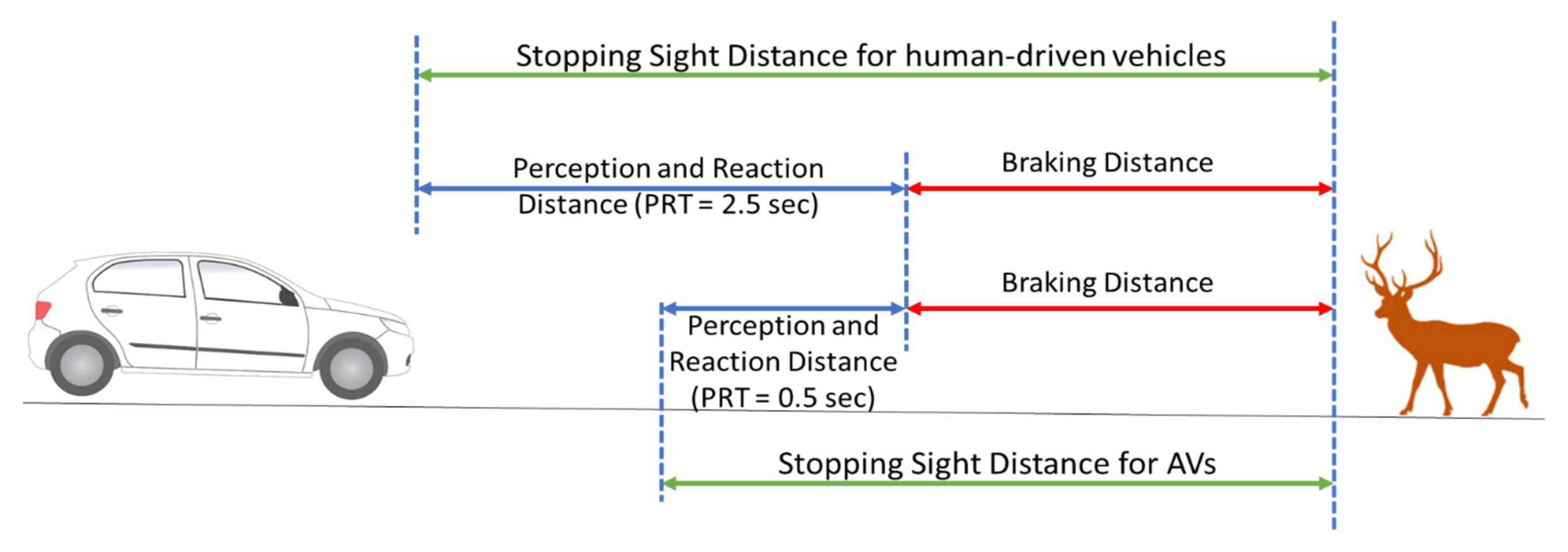
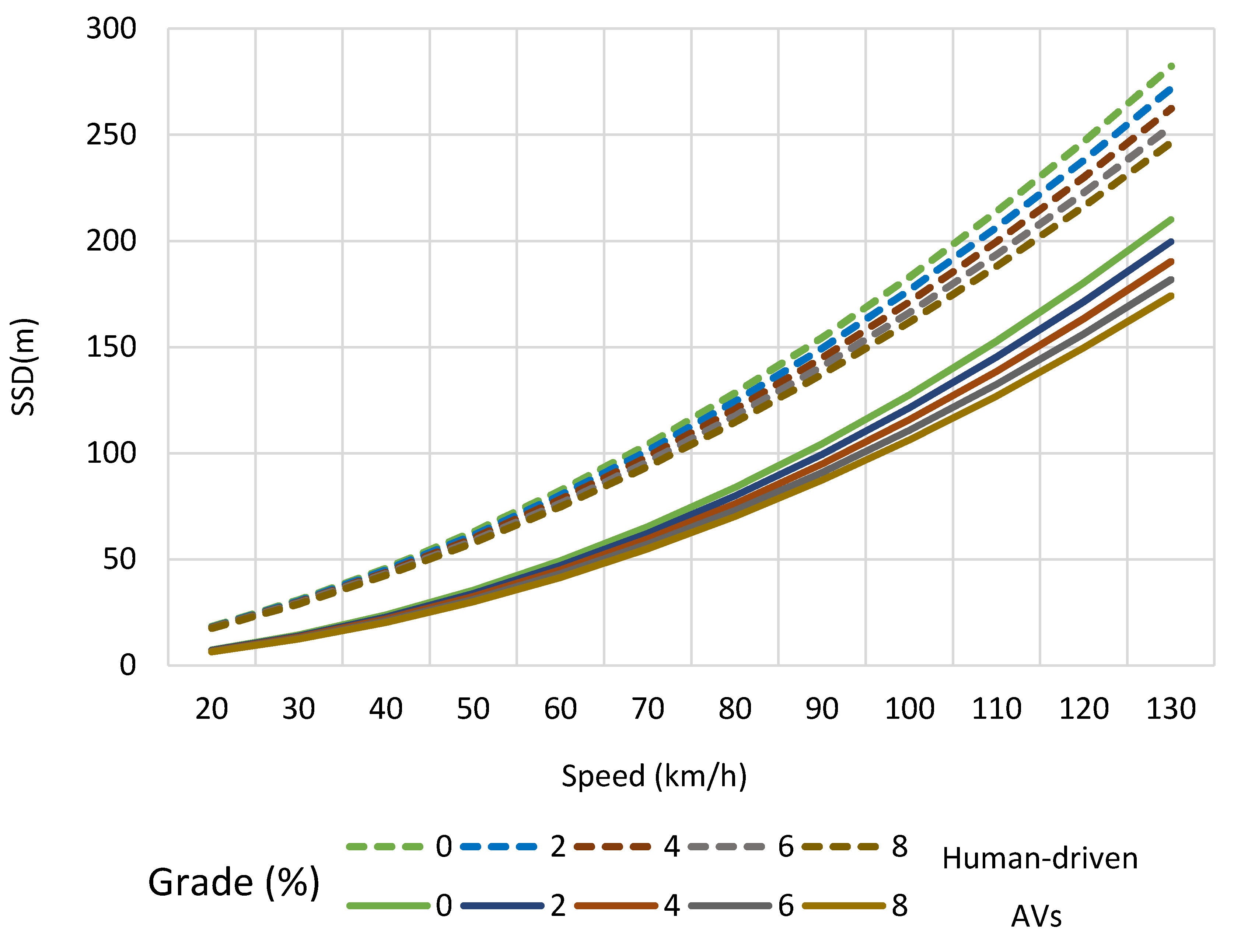
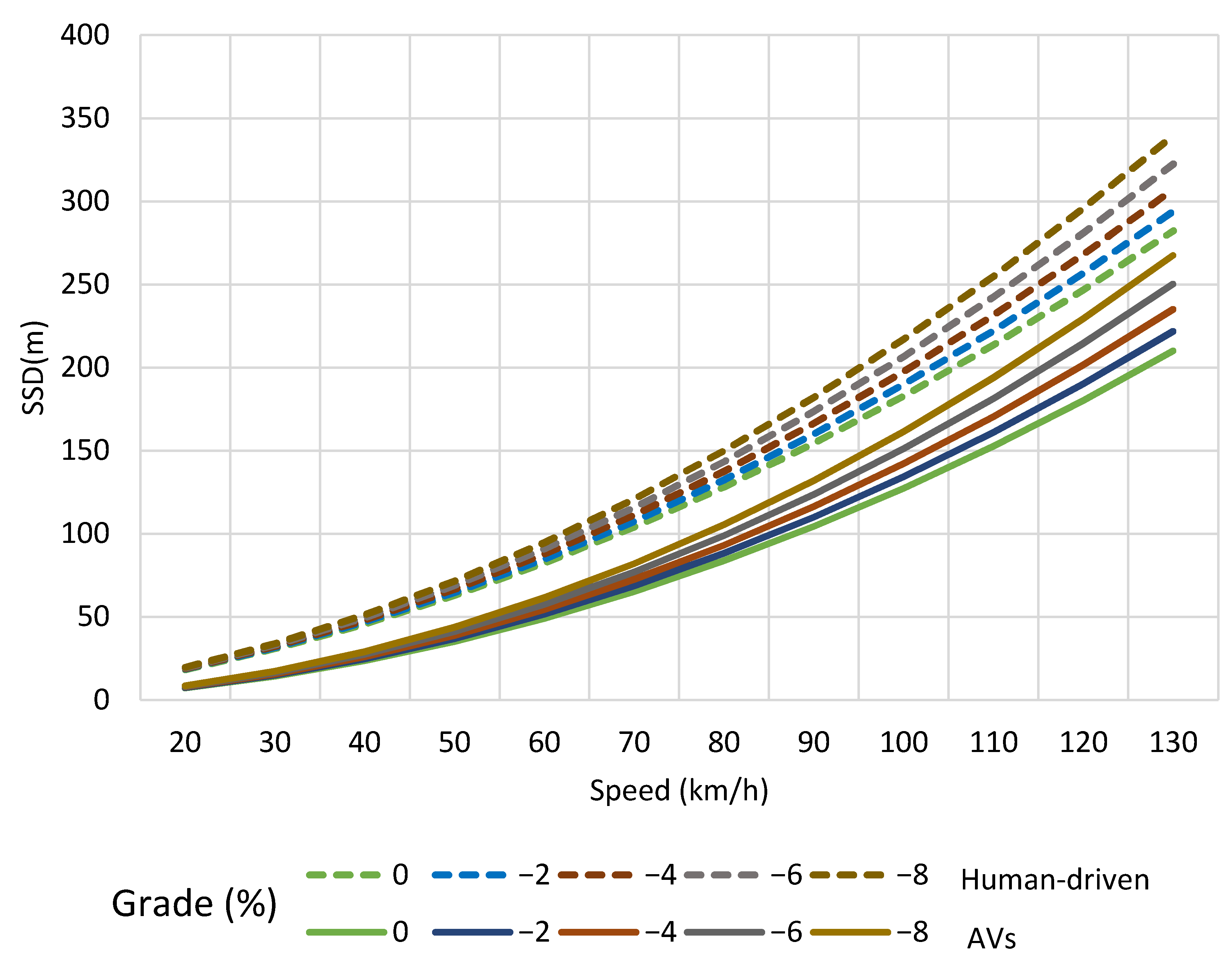
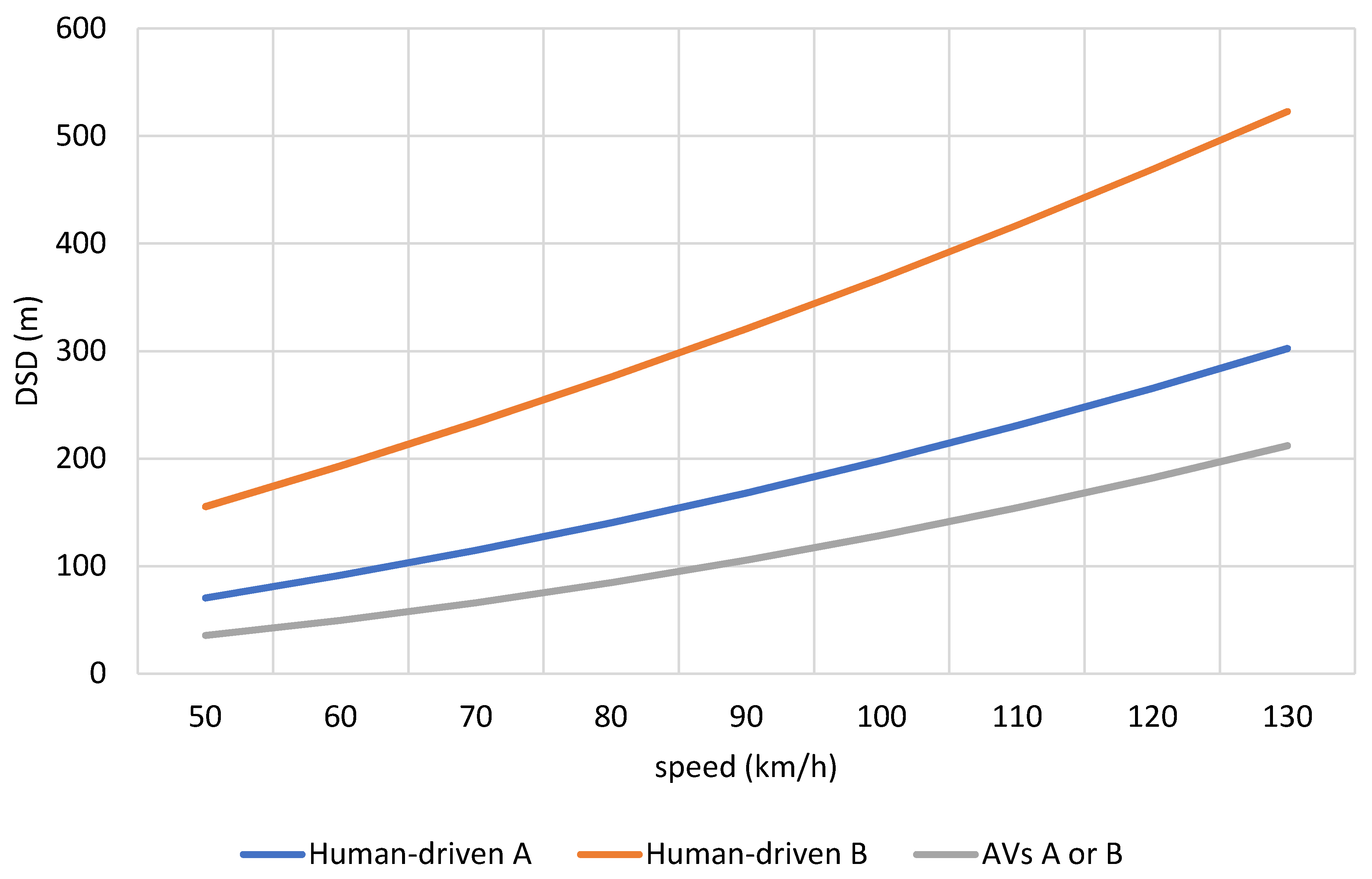
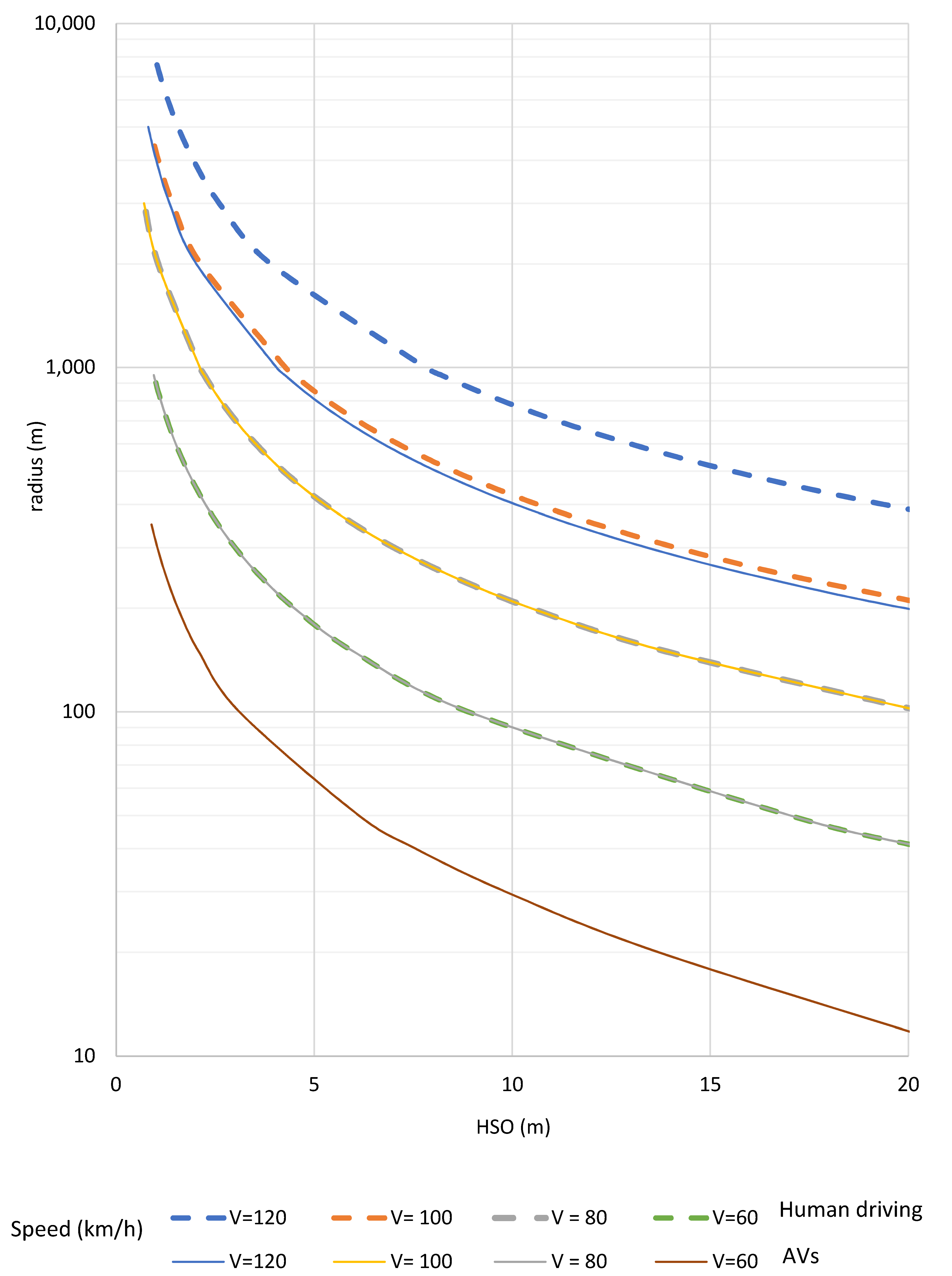
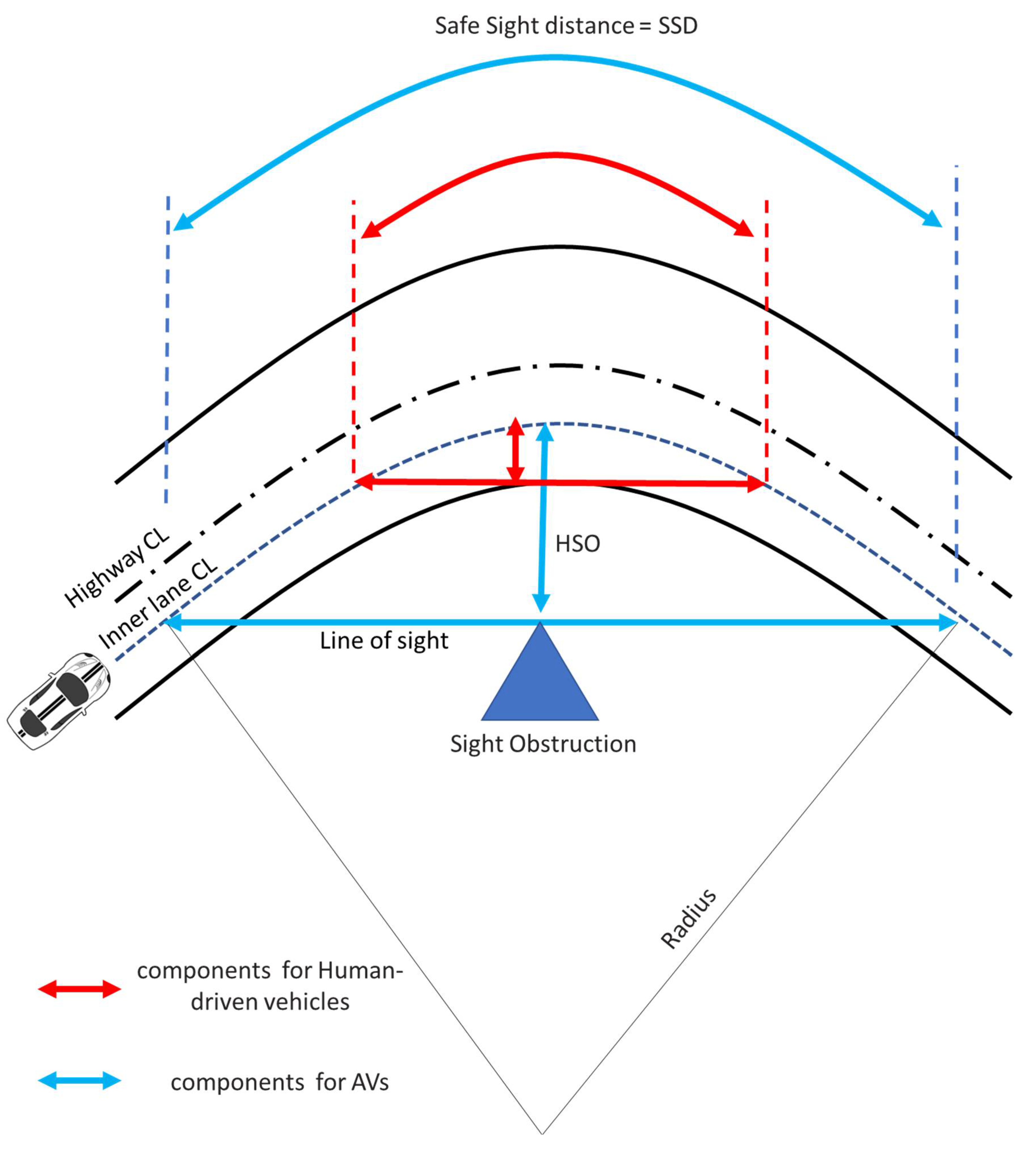
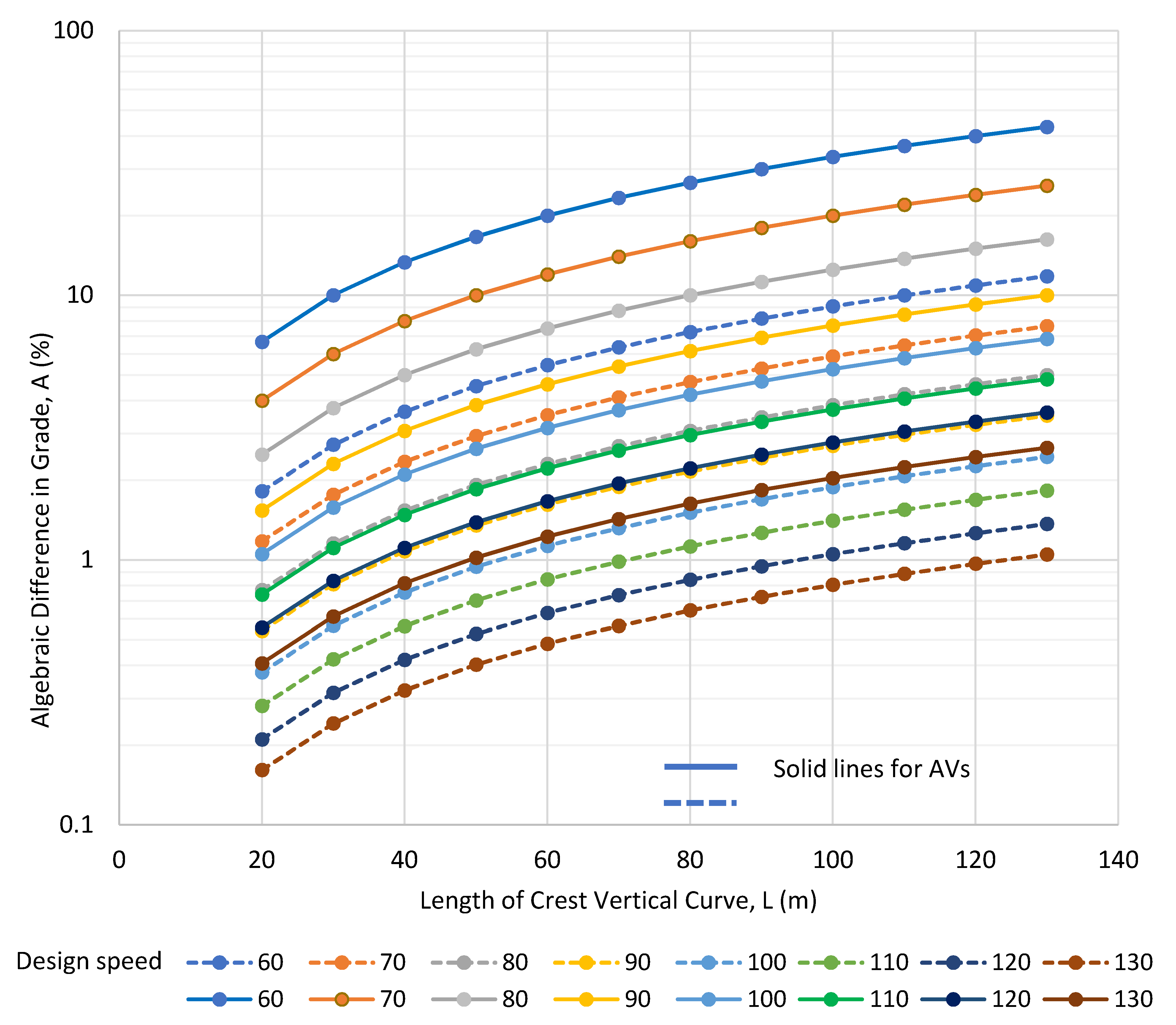
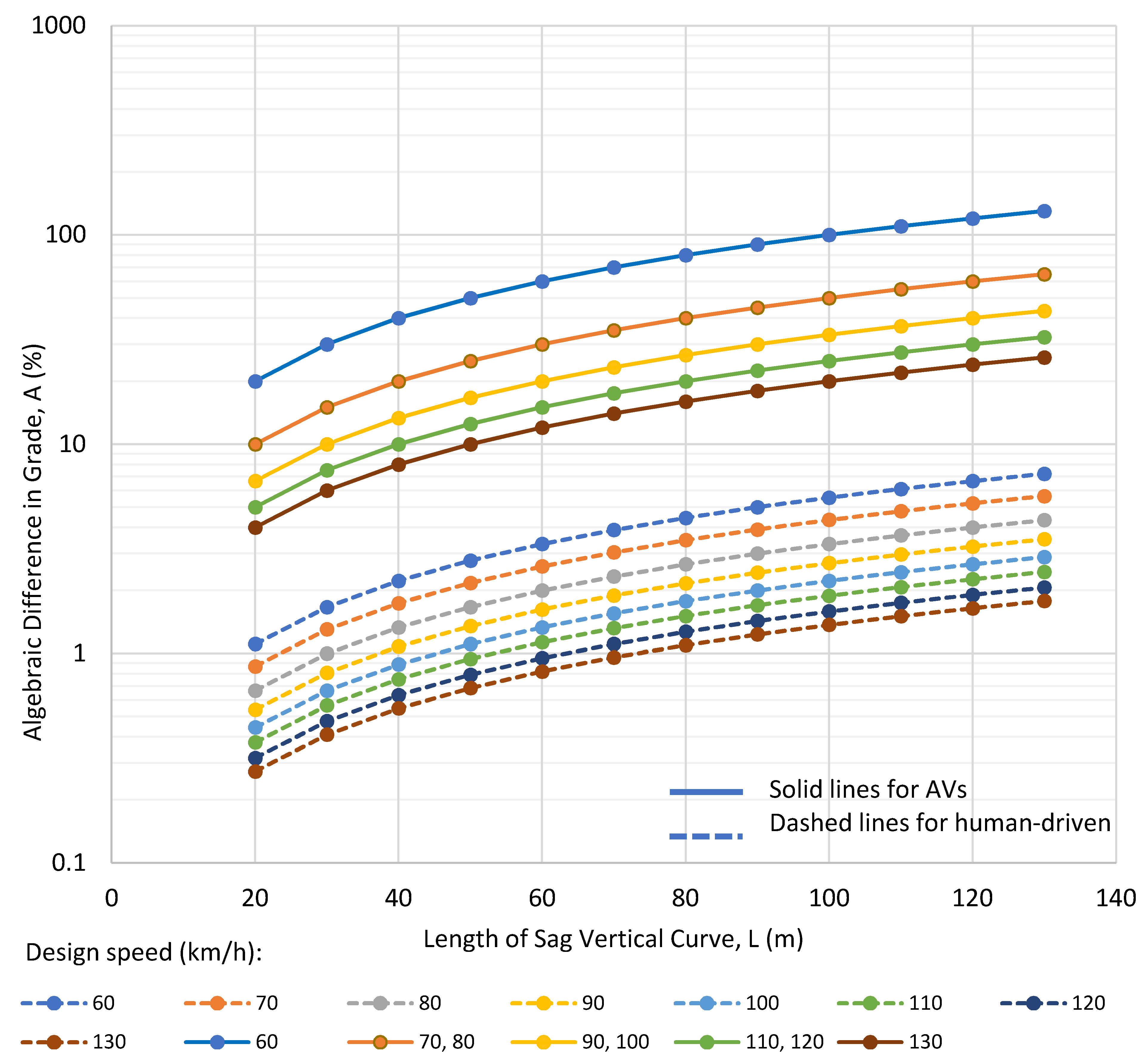
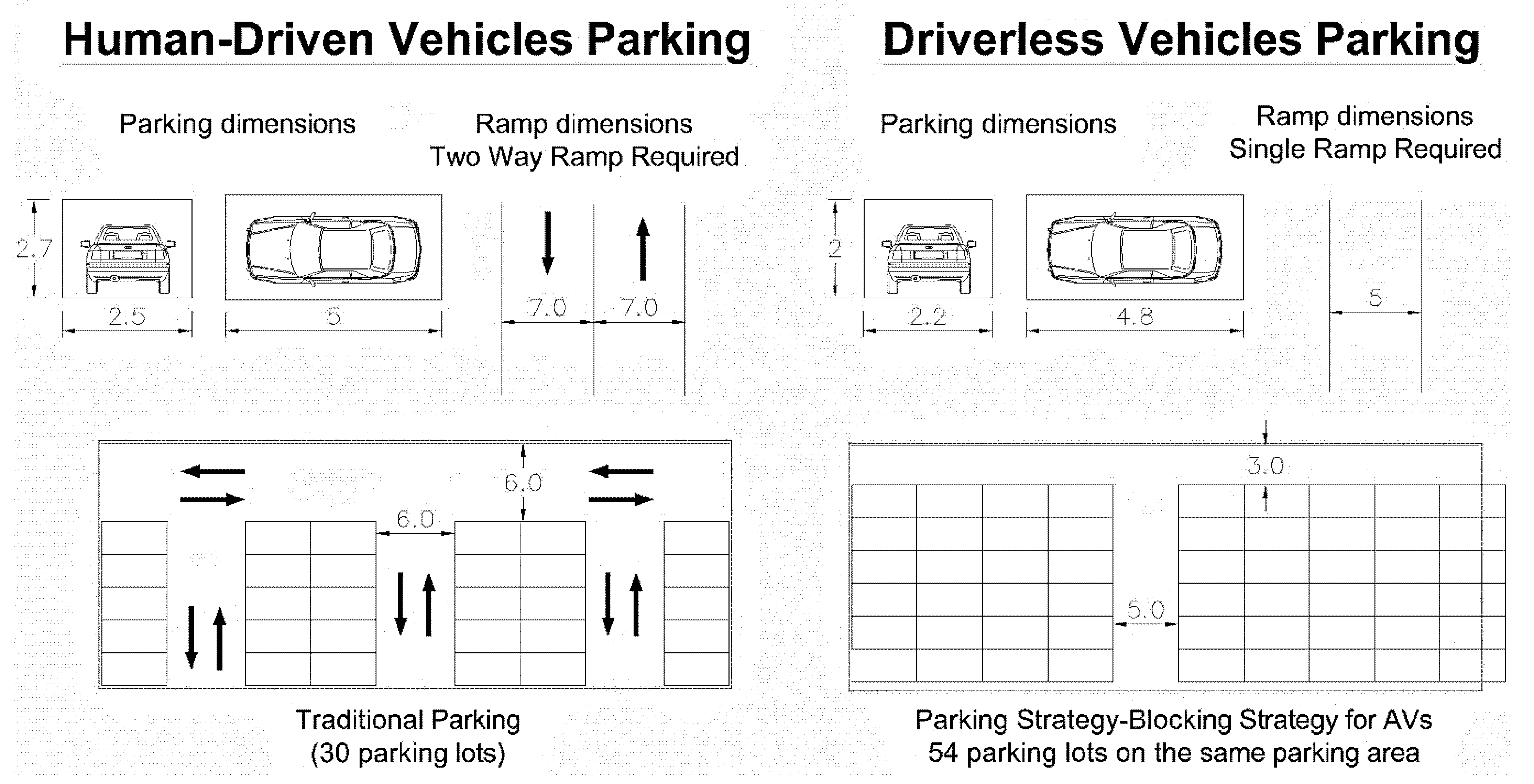
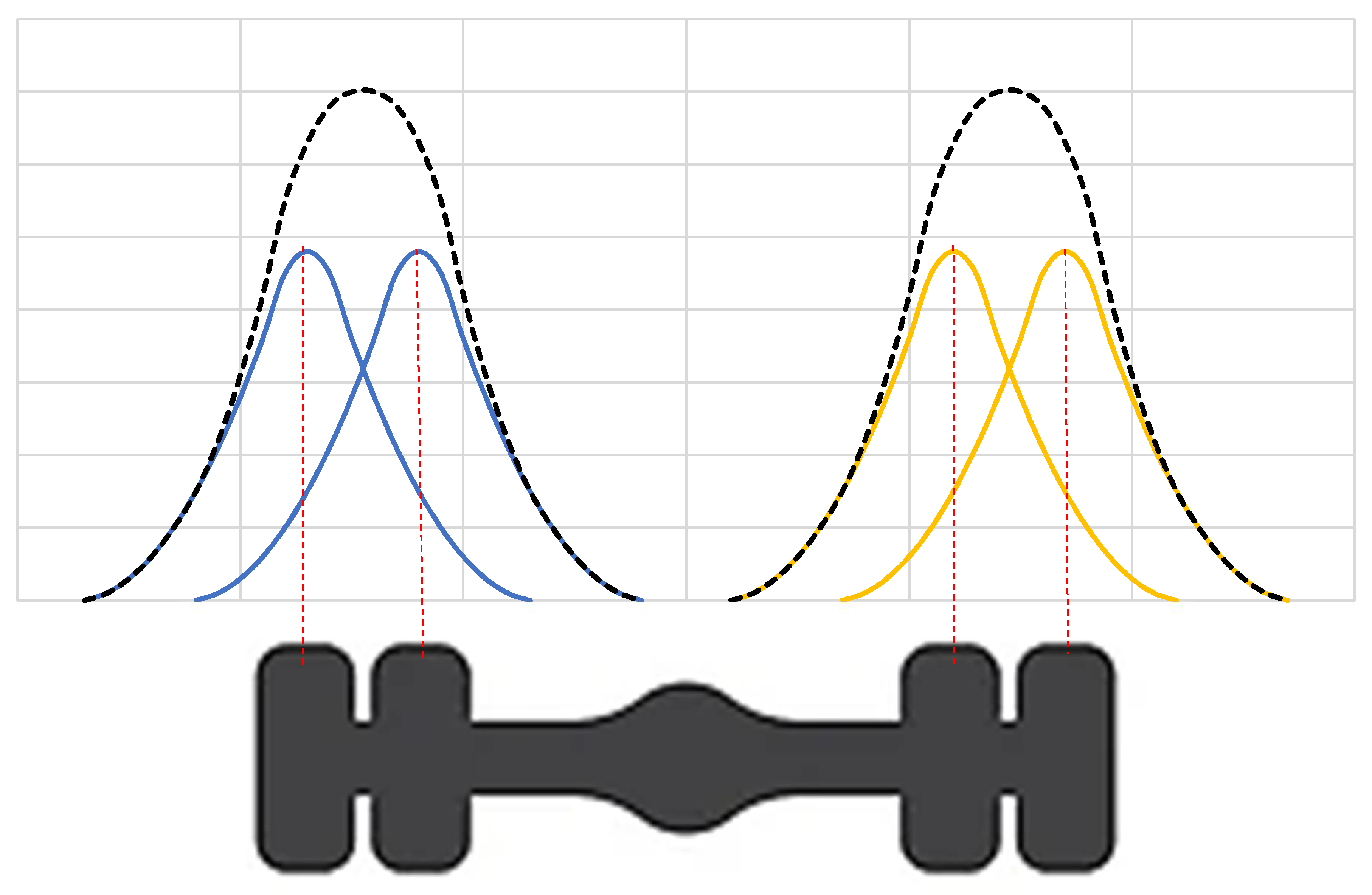
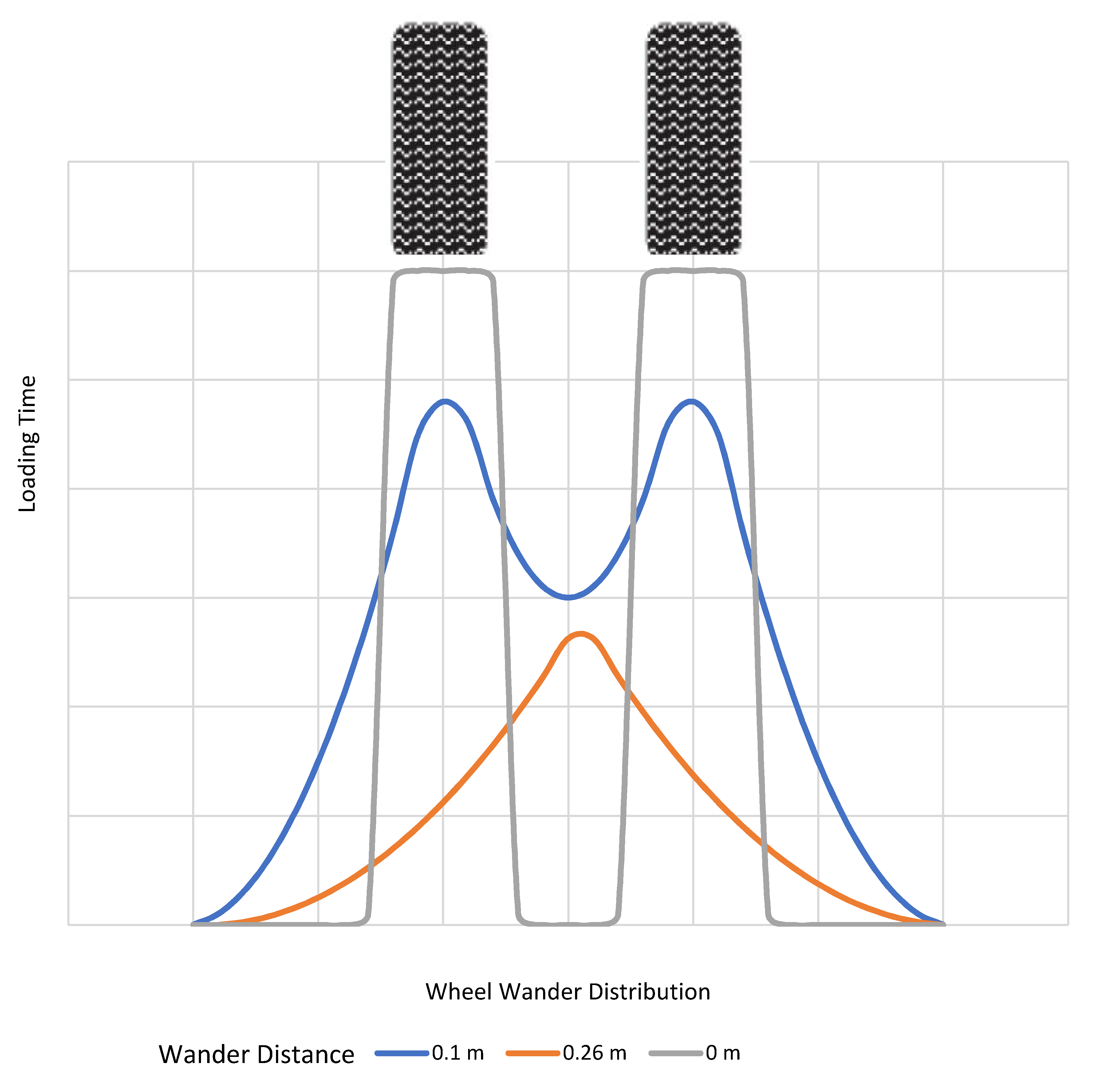
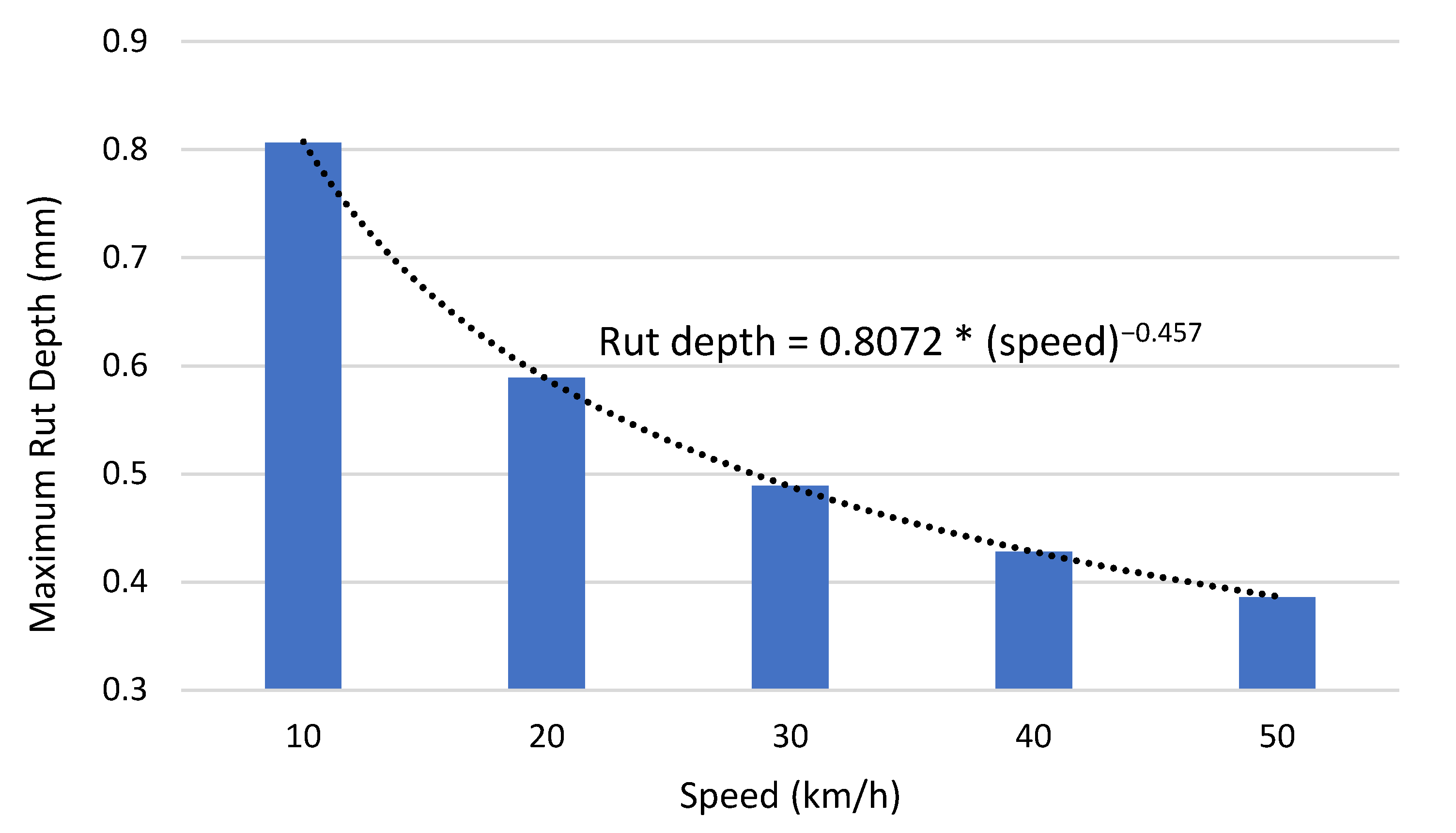
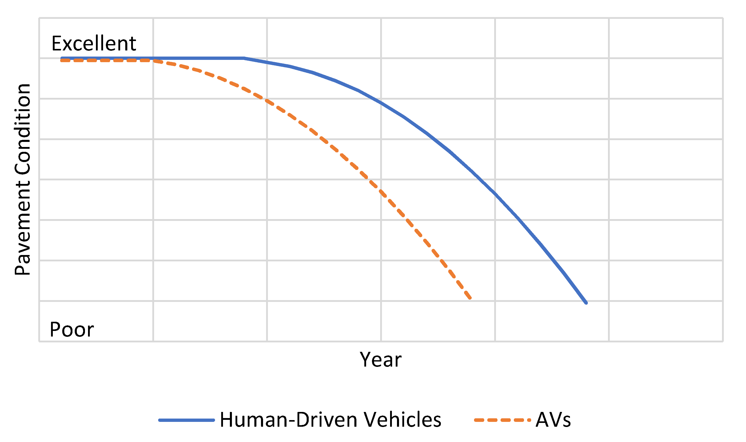
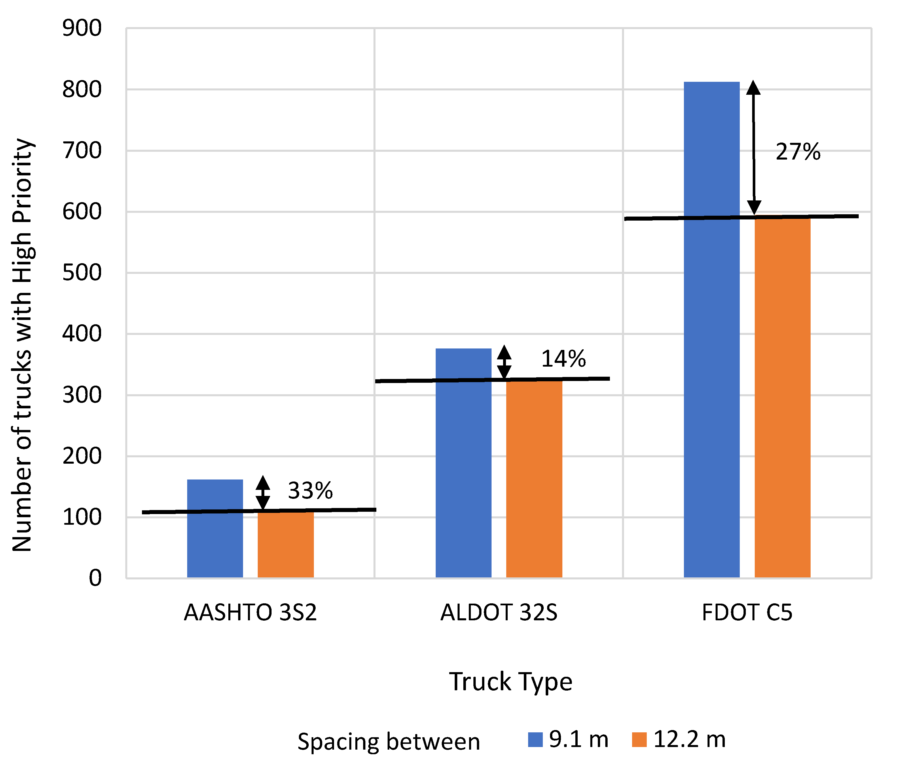
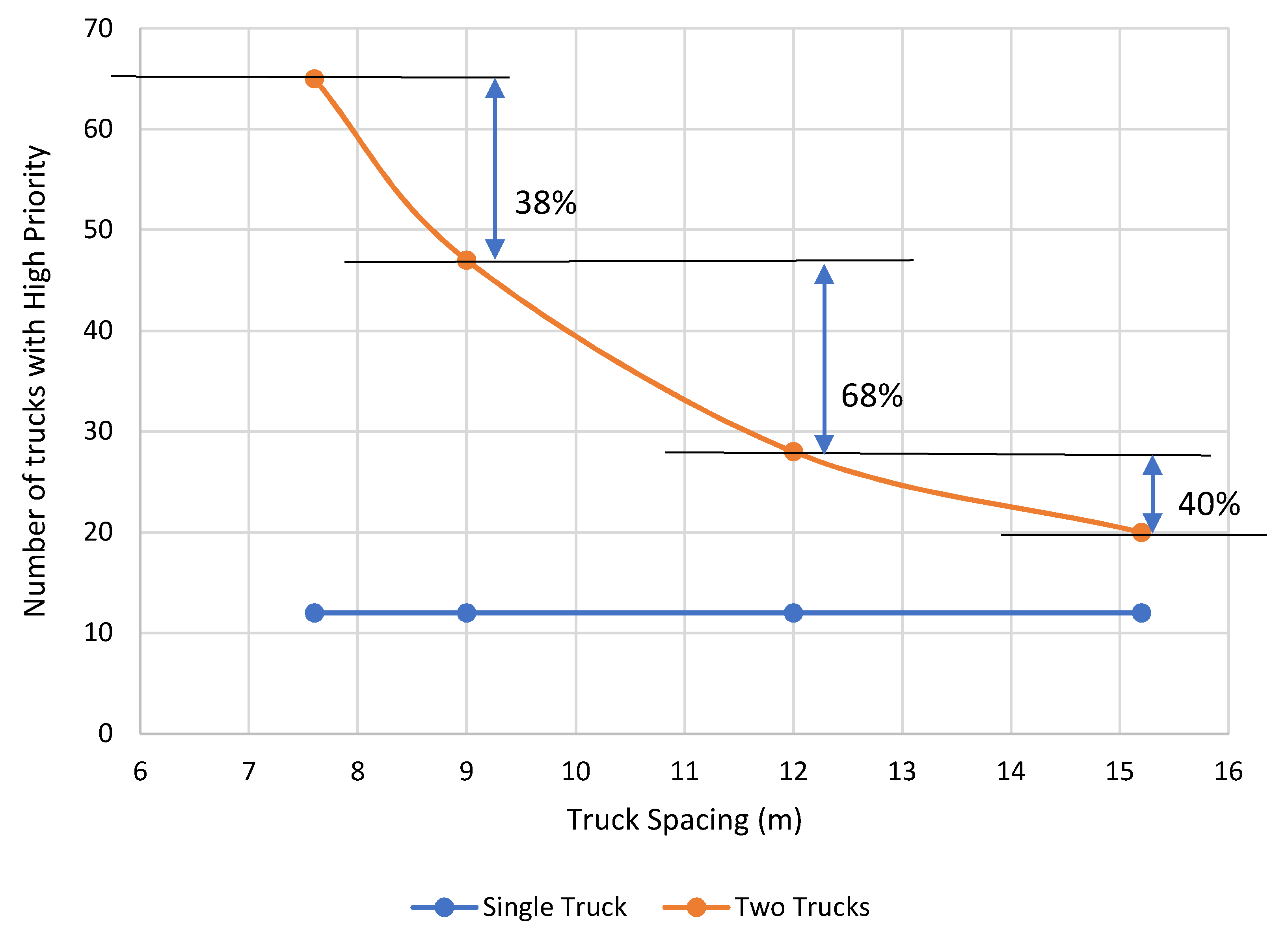
Table 1.
SSD on level roads for human-driven vehicles and autonomous vehicles (AVs).
| Design Speed (km/h) | Human-Driven Vehicles | AVs | SSD Difference (m) | ||||||
|---|---|---|---|---|---|---|---|---|---|
| PRD (m) | Braking Distance (m) | SSD (m) | PRD (m) | Braking Distance (m) | SSD (m) | ||||
| Calculated | Design | Calculated | Design | ||||||
| 20 | 13.9 | 4.6 | 18.5 | 20 | 2.78 | 4.6 | 7.38 | 5 | 15 |
| 30 | 20.9 | 10.3 | 31.2 | 30 | 4.17 | 10.3 | 14.5 | 15 | 15 |
| 40 | 27.8 | 18.2 | 46 | 45 | 5.56 | 18.2 | 23.8 | 25 | 20 |
| 50 | 34.8 | 28.5 | 63.3 | 65 | 6.95 | 28.5 | 35.5 | 35 | 30 |
| 60 | 41.7 | 41 | 82.7 | 85 | 8.34 | 41 | 49.3 | 50 | 35 |
| 70 | 48.7 | 55.9 | 105 | 105 | 9.73 | 55.9 | 65.6 | 65 | 40 |
| 80 | 55.6 | 73 | 129 | 130 | 11.1 | 73 | 84.1 | 85 | 45 |
| 90 | 62.6 | 92.3 | 155 | 155 | 12.5 | 92.3 | 105 | 105 | 50 |
| 100 | 69.5 | 114 | 184 | 185 | 13.9 | 114 | 128 | 130 | 55 |
| 110 | 76.5 | 138 | 214 | 215 | 15.3 | 138 | 153 | 155 | 60 |
| 120 | 83.4 | 164 | 248 | 250 | 16.7 | 164 | 181 | 180 | 70 |
| 130 | 90.4 | 193 | 283 | 285 | 18.1 | 193 | 211 | 210 | 75 |
Table 2.
Decision sight distance for cases A and B for both human-driven vehicles and AVs.
| Design Speed (km/h) | Calculated (m) | Design (m) | ||||
|---|---|---|---|---|---|---|
| Human-Driven | AVs | Human-Driven | AVs | |||
| A | B | A or B | A | B | A or B | |
| 50 | 70.37 | 155.16 | 35.62 | 70 | 155 | 35 |
| 60 | 91.33 | 193.08 | 49.63 | 90 | 195 | 50 |
| 70 | 114.58 | 233.29 | 65.93 | 115 | 235 | 65 |
| 80 | 140.13 | 275.79 | 84.53 | 140 | 275 | 85 |
| 90 | 167.97 | 320.59 | 105.42 | 170 | 320 | 105 |
| 100 | 198.10 | 367.68 | 128.60 | 200 | 370 | 130 |
| 110 | 230.53 | 417.07 | 154.08 | 230 | 415 | 155 |
| 120 | 265.25 | 468.75 | 181.85 | 265 | 470 | 180 |
| 130 | 302.27 | 522.72 | 211.92 | 300 | 525 | 210 |
Table 3.
Formulas for calculating the crest curve length for human-driven vehicles and AVs.
| Human-Driven h1 = 1.08 m h2 = 0.6 m | AVs h1 = 1.84 m h2 = 0.6 m | |
|---|---|---|
| S < L | L = | L = |
| S > L | L = 2S − | L = 2S − |
Table 4.
Design Controls for Crest Vertical Curves Based on Stopping Sight Distance for human-driven and AVs.
Table 4.
Design Controls for Crest Vertical Curves Based on Stopping Sight Distance for human-driven and AVs.
| Desing Speed (km/h) | SSD (m) | K (Calculated) (m) | K (Design) (m) | |||
|---|---|---|---|---|---|---|
| Human-Driven | AVs | Human-Driven | AVs | Human-Driven | AVs | |
| 20 | 20 | 5 | 0.60 | 0.02 | 1 | 1 |
| 30 | 30 | 15 | 1.36 | 0.24 | 2 | 1 |
| 40 | 45 | 25 | 3.07 | 0.68 | 4 | 1 |
| 50 | 65 | 35 | 6.42 | 1.34 | 7 | 2 |
| 60 | 85 | 50 | 10.98 | 2.75 | 11 | 3 |
| 70 | 105 | 65 | 16.75 | 4.65 | 17 | 5 |
| 80 | 130 | 85 | 25.68 | 7.95 | 26 | 8 |
| 90 | 155 | 105 | 36.51 | 12.14 | 37 | 13 |
| 100 | 185 | 130 | 52.01 | 18.61 | 53 | 19 |
| 110 | 215 | 155 | 70.25 | 26.45 | 71 | 27 |
| 120 | 250 | 180 | 94.98 | 35.68 | 95 | 36 |
| 130 | 285 | 210 | 123.44 | 48.56 | 124 | 49 |
Table 5.
Formulas for calculating the sag curve length for human-driven vehicles and AVs.
| Human-Driven H = 0.6 m = 1 | AVs H = 0.84 m = 13.4 | |
|---|---|---|
| S < L | L = | L = |
| S > L | L = 2S − | L = 2S − |
Table 6.
Design Controls for Sag Vertical Curves Based on Stopping Sight Distance for human-driven and AVs.
Table 6.
Design Controls for Sag Vertical Curves Based on Stopping Sight Distance for human-driven and AVs.
| Desing Speed (km/h) | SSD (m) | K (Calculated) (m) | K (Design) (m) | |||
|---|---|---|---|---|---|---|
| HD | AVs | HD | AVs | HD | AVs | |
| 20 | 20 | 5 | 2.10 | 0.04 | 3 | 1 |
| 30 | 30 | 15 | 4 | 0.20 | 4 | 1 |
| 40 | 45 | 25 | 7.29 | 0.39 | 8 | 1 |
| 50 | 65 | 35 | 12.15 | 0.59 | 13 | 1 |
| 60 | 85 | 50 | 17.30 | 0.90 | 18 | 1 |
| 70 | 105 | 65 | 22.61 | 1.21 | 23 | 2 |
| 80 | 130 | 85 | 29.39 | 1.62 | 30 | 2 |
| 90 | 155 | 105 | 36.26 | 2.03 | 37 | 3 |
| 100 | 185 | 130 | 44.59 | 2.55 | 45 | 3 |
| 110 | 215 | 155 | 52.97 | 3.07 | 53 | 4 |
| 120 | 250 | 180 | 62.81 | 3.59 | 63 | 4 |
| 130 | 285 | 210 | 72.68 | 4.22 | 73 | 5 |
Table 7.
Summary of the proposed lane width for AVs from across different studies.
| Study | Proposed Lane Width | Ref. |
|---|---|---|
| Machiani, S. et al. (2021) | The lane width can be 8 to 9 feet in the era of AVs | [52] |
| Schlossberg, M. et al. (2018) | Reduce the lane width to 8 feet instead of 12 feet for human-driven vehicles | [53] |
| Aryal, P. (2020) | The lane width can be reduced to 8 or 9 feet and in freeways the lane width can be reduced to 9 feet instead of 12 feet for human-driven vehicles. | [54] |
| Snyder, R. (2018) | The lane width can be reduced by 20–25% of the current lane width of the road | [55] |
| Heinrichs, D. (2016) | 8 to 9 feet lane width will be enough for AVs | [56] |
| Hafiz and Zohdy (2021) | The lane width can be reduced to 2.5 m instead of 3.6 m for human-driven vehicles | [57] |
| McCarville, I. (2019) | The required lane width can be reduced to 8 feet | [58] |
Publisher’s Note: MDPI stays neutral with regard to jurisdictional claims in published maps and institutional affiliations. |
© 2021 by the author. Licensee MDPI, Basel, Switzerland. This article is an open access article distributed under the terms and conditions of the Creative Commons Attribution (CC BY) license (https://creativecommons.org/licenses/by/4.0/).
Share and Cite
MDPI and ACS Style
Othman, K. Impact of Autonomous Vehicles on the Physical Infrastructure: Changes and Challenges. Designs 2021, 5, 40. https://0-doi-org.brum.beds.ac.uk/10.3390/designs5030040
AMA Style
Othman K. Impact of Autonomous Vehicles on the Physical Infrastructure: Changes and Challenges. Designs. 2021; 5(3):40. https://0-doi-org.brum.beds.ac.uk/10.3390/designs5030040
Chicago/Turabian StyleOthman, Kareem. 2021. "Impact of Autonomous Vehicles on the Physical Infrastructure: Changes and Challenges" Designs 5, no. 3: 40. https://0-doi-org.brum.beds.ac.uk/10.3390/designs5030040