Article

A Probabilistic Approach to the Spatial Variability of Ground Properties in the Design of Urban Deep Excavation

1
Department of Computing and Engineering, University of East London, London E16 2RD, UK
2
Fairhurst, Newcastle Upon Tyne NE4 6DB, UK
3
bei AECOM, 45127 Essen, Germany
4
MESLEC Ltd., Elstree WD6 3DP, UK
5
Faculty of Engineering, Civil Engineering Department, Urmia University, Urmia 5756151818, Iran
*
Author to whom correspondence should be addressed.
Submission received: 30 June 2019 / Revised: 29 July 2019 / Accepted: 8 August 2019 / Published: 12 August 2019
(This article belongs to the Special Issue Advances in Dam Engineering)

Abstract

:
Uncertainty in ground datasets often stems from spatial variability of soil parameters and changing groundwater regimes. In urban settings and where engineering ground interventions need to have minimum and well-anticipated ground movements, uncertainty in ground data leads to uncertain analysis, with substantial unwelcomed economical and safety implications. A probabilistic random set finite element modelling (RSFEM) approach is used to revisit the stability and serviceability of a 27 m deep submerged soil nailed excavation built into a cemented soil profile, using a variable water level and soil shear strength. Variation of a suite of index parameters, including mobilized working loads and moments in facing and soil inclusion elements, as well as stability and serviceability of facing and the integrated support system, are derived and contrasted with field monitoring data and deterministic FE modelling outputs. The validated model is then deployed to test the viability of using independent hydraulic actions as stochastic variables as an alternative to dependent hydraulic actions and soil shear strength. The achieved results suggest that utilizing cohesion as a stochastic variable alongside the water level predicts system uncertainty reasonably well for both actions and material response; substituting the hydraulic gradient produces a conservative probability range for the action response only.

Graphical Abstract

1. Introduction

Rapid and sustained urban sprawl is expected to continue to accommodate an estimated 70% of the world population in cities by 2050 [1]. Exploitation of the urban sub-surface has attracted increasing attention in the past 50 years as a solution to a shortage of space and services per head, and is reflected, nationally and internationally, in many current planning policies, including [2] in the UK. Ground movements arising from deep excavation need to be strictly limited to permissible levels; that is, to be controlled through design and deployment of top-down support of excavation systems that allow prevention and mitigation of excessive ground movements from the outset. In an urban context and where the subsurface is already congested (by buried utilities and underground structures), any further disturbance can lead to variations in groundwater conditions, with immediate implications on some soil engineering properties. Spatial variability of shallow disturbed ground and limited space for intrusive ground investigation, as well as extreme climates that reportedly cause a broad range of problems, including fatigue [3] and mineral dissolution [4], add to the uncertainty and cast doubt on the reliability of the estimated stability and serviceability of support systems. At a practical level, these systems are commonly designed through deterministic analysis of engineered grounds using ground properties that are statistically moderated, and in the context of some standards, further factored down by an arguably arbitrary partial factor.
Ideally, support systems should be adaptive in allowing improved integration with the variable ground and groundwater conditions during the course of construction and also the service life. Use of arbitrary safety factors fall short in satisfying that integration. This paper studies the scopes for using an alternative statistical design approach, with an attempt to incorporate likely scenarios of actions and material properties into design within the context of an urban deep basement case study. The framework may be adopted as an alternative to arbitrary partial and safety factors. Stochastic discretization of random fields is used to determine and incorporate into finite element (FE) analysis sets of random variables to revisit a monitored 28 m deep submerged soil nail system. Effects of actions and serviceability are determined and reported in lower-bound to upper-bound ranges, and alongside, the most likely indexes (for structure performance) are contrasted, with outcomes of commonly practiced deterministic FE and FHWA-compliant [5] design. Two sets of stochastically dependent (water level and true cohesion) variables are initially used to verify the framework. Further analysis is presented using two sets of stochastically independent (water level and hydraulic gradient) variables to test the viability of different input variables.

2. Risk and Probabilistic Analysis in the Geotechnical Context

Naturally occurring materials, such as soil, are inherently variable. The uncertainty increases in space and upon ground disturbance, or in dynamic constantly changing total environments. National codes of practice allow statistical evaluation methods for determination of characteristic ground properties. The common universal practice is to factor down the ground resistance index parameters, statistically moderated ground properties, or a combination of the two using sets of partial factors that are predetermined and rather arbitrary. Whilst previous experience can be used as a basis for adopted factors of safety [6], this conservative approach falls short in addressing the impacts of spatial variability on computer reliability.
The probabilistic approach in geotechnical design has not received much interest, with stimulus from two directions: The mathematical structure of probabilistic approaches is often not appealing to practicing engineers; and the general perception is that probabilistic analysis incurs more time and cost. Early models include the first order second moment (FOSM) from Taylor Series and based on Bayes rule [7,8]; the method did not receive much attention mainly due to its inconsistency with non-linear functions [9]. Monte Carlo simulation in geotechnics was introduced and discussed in a series of seminal works [10,11], with limitations revisited more recently in [12]. Early attempts into the use of random set (RS) theory in geomechanics include the work of [13,14,15] in the design of linings for tunnels into rock. The RS framework was first used in conjunction with finite element (FE) analysis in [16].

3. Benchmark Problem and Methods

3.1. Benchmark Problem

The benchmark problem used in this contribution is a 28 m deep vertical cut in 2 to 2.5 m high lifts, from ground surface at 104.7 m above ordnance datum (mAOD) to 76.65 mAOD, and supported with a top-down soil nail system in a heavily built setting [17]. Figure 1 shows a cross-section diagram of the supported excavation, and adjoining features. Figure 1 shows the variation of the water level at the face of the excavation and also the hydraulic gradient, during the course of excavation. A 40 m long section was adopted for the purpose of this paper, where the land terrain led to a maximum depth of excavation. The cut was excavated into seven soil layers and supported with three flexible reinforced shotcrete facings, divided with two 2 m wide soil benches, and 13 rows of soil nails, 6 to 14 m long, installed at a 10° to 25° inclination. Soil nail elements included 28 to 32 mm steel bars installed centrally in 700 to 850 mm drilled holes that were eventually filled with a sand-cement grout. The soil nails were spaced 2 to 2.5 m horizontally and 1.5 to 3 m vertically. The cut was benched at 10.04 and 17.04 mbgl. A series of 4 to 6 m long, 4-inch drain perforated PVC pipes were installed at 10° elevations, at 3.10, 6.10, and 8.35 m from the bed of excavation. Drains were connected by series of 0.3 m wide vertical geocomposite blankets installed between shotcrete facing and retained ground from 87.0 to 76.65 mAOD. An evenly distributed 49 kPa permanent surcharge (20 m run) was applied 12 m from the excavation crest, representing the contact pressure from the neighbouring six-storey residential buildings. Piezometric readings derived from the ground investigation report [17] indicate a southward flow of groundwater, with a natural hydraulic gradient ranging from 0.1 to 0.2 (i.e., 1 to 2 m drop in every 10 m running perpendicular to project line—see Figure 1). The water level varied from 84.5 to 91.2 mAOD prior to construction. The system was designed for a mean 88 mAOD water level. Although commonly practiced, this is a substantial simplification, which reportedly led to excessive seepage and lateral displacement during the course of the staged excavation. Lateral ground movements were recorded using laser inclinometers at reflectors installed at 97 mAOD, five times each month to the end of the excavation. The northern wall section (covered by nine reflectors) was used for the purpose of this study, showing a cumulative lateral displacement of 115 mm, and a 61 mm horizontal displacement six months post-construction.

3.1.1. Materials

The benchmark site is located in North Tehran and is composed of Quaternary (Pleistocene) permeable dark reddish to yellowish brown cemented poorly sorted alluvium (Bn fm). Table 1 summarizes the ground stratification, and mean (i.e., characteristic) long-term strength, stiffness, and hydraulic properties of soil layers in the benchmark site. The influence of construction and groundworks on soil properties is indisputable but was not considered either in the original design or in the present probabilistic analysis. Whilst this counts as a limitation, it allows study of the influence on actions and ground properties of seasonal groundwater regimes only.
Granular soils form the top 18 m of the ground profile in the project site. The granular layers are generally cemented with hardly soluble calcite nodules; the clay fraction increases with depth and begins to control the overall soil behaviour from about 18 mbgl (meters below ground level) down to 29 mbgl. For the entire profile, the plasticity index ranges within the narrow range of 10% to 20% (i.e., low plasticity), with a Standard Penetration Number of >50, highlighting the role of calcite cementation. Piezometer readings over 7 months ahead and during the construction (May to November) showed a fluctuating water level from 11.5 to 18 mbgl (91.2 to 84.5 mAOD) on the project line; this was attributed in part to the natural terrain of the land and seasonal precipitation. The soil nail system was originally designed for a conservative 85.7 mAOD water level. Variations of the water level have direct implications on layer 4 (cemented sand) and level 5 (low-plasticity clay), and extend through the capillary rise effect to layers 2 and 3. The impacts of capillary rise were evident from the variable water content within soil layers 2 and 3.

3.1.2. Plaxis 2D Model

The nonlinear finite elements (FE) method was used to allow simulation of staged (sequenced) construction, soil–structure interaction, and steady-state flow, and also to allow measurement of mobilized stresses and deformations by the end and during the course of construction. Deterministic analysis was undertaken using the Plaxis 2D software. The soil layers were modelled using 15-node triangular elasto-plastic plain-strain finite elements. The local element factor was reduced to 0.1 for areas around drains to allow steady-state flow analysis. The Mohr-Coulomb failure criterion was adopted. Reinforced shotcrete flexible facing was modelled using elastic beam elements, with interface elements featuring a reduced 5% shear capacity (Rint = 0.95) compared to the surrounding soil. Elasto-plastic plate elements were preferred over geogrid elements to incorporate into the analysis the impact of the bending stiffness of steel bars and the nail-facing joint as a rigid connection. The axial and bending stiffness of plates was normalized against the horizontal nail spacing and are presented in Table 2 for drill holes of a 0.08 m diameter. Standard fixities were applied to horizontal and vertical boundaries. Drain elements contained five nodes and were assigned a head to represent every stage of excavation. The Phi/C (strength) reduction method was adopted to analyse the stability of the system at each stage and at the end of construction. Tolerance was limited to 1%; a maximum of 50 steps were deemed sufficient in determining the global factor of safety.

3.2. Probabilistic Framework

Random fields were employed to formulate the variability of actions and material properties in a probabilistic framework. Three variables were paired into sets of stochastically dependent and stochastically independent parameters to first study the general impact on the serviceability and stability of uncertain input parameters, and then to seek the difference between two variable pairs and impacts on design.
To study the impact of water level variation and subsequent alterations to the apparent cohesion of cemented soils (i.e., design scenario 1: Stochastically dependent variables), random set realizations were defined using two datasets of equal probability (Table 3). Water level and cohesion were varied from the lower-bound to the upper-quartile in the first dataset; and from the lower-quartile to the upper-bound in the second dataset. A further two input data sets were defined using a stochastically independent hydraulic gradient and water level (i.e., design scenario 2) to revisit the stability and performance of the support system (Table 3).
The water level was varied to match the captured fluctuations through the construction time, between 79.75 to 88 mAOD (i.e., 16 to 24.3 mbgl); the discharge rate at the face of excavation, representing a hydraulic gradient range of 0.1 to 0.2, was also varied. The hydraulic gradients were assigned to the model by introducing a head different between the phreatic line—cut intercept and the vertical model boundary. A head difference of 1V:10, 1.5V:10, and 2F.0V:10 H simulated hydraulic head gradients of 0.1, 0.15, and 0.2, respectively. For the water level to adapt itself during excavation with the location of drain points, a set of representative fixed hydraulic head values were assigned to drain points and the model’s boundary for every phase of submerged excavation. The flow of the groundwater was stemmed from the natural hydraulic gradient, submerged excavation, and activation of drains. On the FE model, this condition was met by drawing inclined water levels and performing groundwater flow calculation. Interface elements were activated during the groundwater flow calculation to prevent flow through the wall.
The total number of realisations required to run a meaningful random set analysis is outlined through Equation (1) [18]:
N c = 2 n i = 1 N n i
where N is the number of basic variables and n i the number of sources available for each variable. Therefore, with a total of two basic variables, 16 realisations are required for random set analysis, outlining the data that feeds the cumulative probability distribution function in the form of probability boxes (i.e., p-box). It does mean that increasing the number of variables increases the output exponentially, therefore a thorough sensitivity analysis to identify critical parameters is generally advised. Focusing solely on univariates from the data sets, Figure 2 presents four p-boxes, highlighting the upper and lower bounds for each variable.
For u = ( x 1 , , x n ) , where x i is the variables, n is the total number of variables, and u is the vector of set value parameters, a random relationship can be defined in the Cartesian form of x 1 × × x n . This renders a vector of combinations of basic variables. In this research, two basic variables are deployed to form four combinations of basic variables; these are discussed in Section 3.2.1 and Section 3.2.2 for two design scenarios.

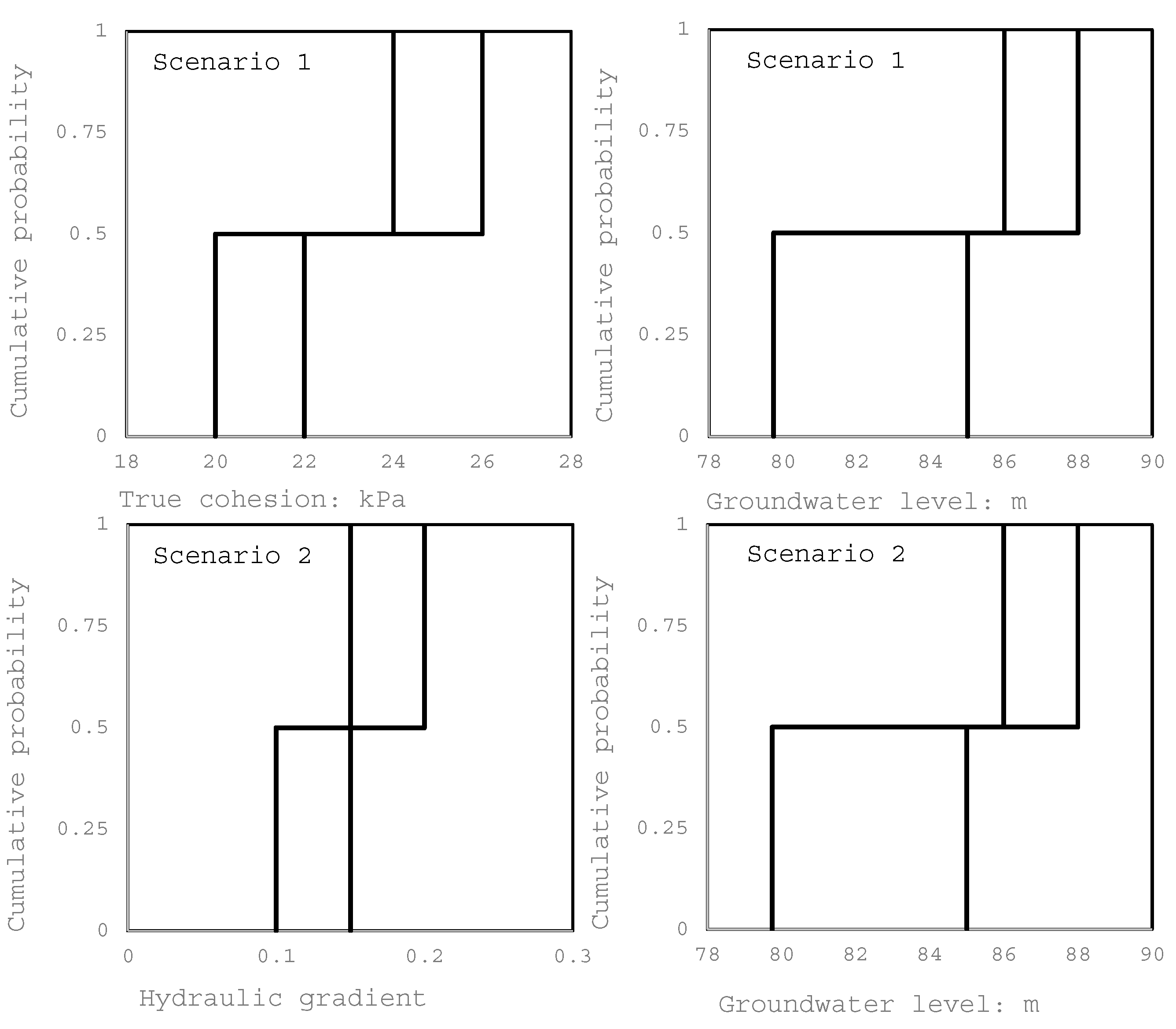
3.2.1. Design Scenario 1

Drained cohesion (C’) and water level (G) were adopted as variables and used to build two random sets. The combined relationship between the two variables was presented in the form of a vector and defined by the 16 realisations arranged into four combinations, as illustrated in Equation (2) (below):
G × C = { ( G 1 , C 1 ) 1 , ( G 2 , C 1 ) 2 , ( G 1 , C 2 ) 3 , ( G 2 , C 2 ) 4 }       = [ G 1 , L L , i 1 , L L G 2 , L L , i 1 , L L G 1 , L L , i 2 , L L G 2 , L L , i 2 , L L G 1 , L U , i 1 , L U G 2 , L U , i 1 , L U G 1 , L U , i 2 , L U G 2 , L U , i 2 , L U G 1 , U L , i 1 , U L G 2 , U L , i 1 , U L G 1 , U L , i 2 , U L G 2 , U L , i 2 , U L G 1 , U U , i 1 , U U G 2 , U U , i 1 , U U G 1 , U U , i 2 , U U G 2 , U U , i 2 , U U ]       = [ 79.75 , 20 86 , 20 79.75 , 22 86 , 22 76.75 , 24 86 , 24 79.75 , 26 86 , 26 85 , 20 85 , 24 88 , 20 88 , 24 85 , 22 88 , 22 85 , 26 88 , 26 ]
where G is water level, C is cohesion, L denotes the lower bound, and U denotes the upper bound.

3.2.2. Design Scenario 2

Hydraulic gradient (i) and water level (G) were adopted as variables and used to build two random sets. The combined relationship between the two variables was presented in the form of a vector and defined by the 16 realisations arranged into four combinations, as illustrated in Equation (3):
G × i = { ( G 1 , i 1 ) 1 , ( G 2 , i 1 ) 2 , ( G 1 , i 2 ) 3 , ( G 2 , i 2 ) 4 }       = [ G 1 , L L , i 1 , L L G 2 , L L , i 1 , L L G 1 , L L , i 2 , L L G 2 , L L , i 2 , L L G 1 , L U , i 1 , L U G 2 , L U , i 1 , L U G 1 , L U , i 2 , L U G 2 , L U , i 2 , L U G 1 , U L , i 1 , U L G 2 , U L , i 1 , U L G 1 , U L , i 2 , U L G 2 , U L , i 2 , U L G 1 , U U , i 1 , U U G 2 , U U , i 1 , U U G 1 , U U , i 2 , U U G 2 , U U , i 2 , U U ]       = [ 79.75 , 0.1 86 , 0.1 79.75 , 0.15 86 , 0.15 76.75 , 0.15 86 , 0.15 79.75 , 0.2 86 , 0.2 85 , 0.1 85 , 0.15 88 , 0.1 88 , 0.15 85 , 0.15 88 , 0.15 85 , 0.2 88 , 0.2 ] ,
where, G is the groundwater level, i is the hydraulic gradient, L denotes the lower bound, and U denotes the upper bound.
Series of FE computations were performed to accommodate the entire random set of realizations using the Plaxis 2D code and outputs, including stresses, strains, and moments, for the structural element and the system as a whole were collated. These were presented on probability boxes and in terms of the lower and upper bounds, allowing the FE outputs to be contrasted with the deterministic FE analysis results, in-situ measurements, or equivalent parameters calculated in compliance with common codes of practice (i.e., ultimate and serviceability limit states).

3.3. Ultimate and Serviceability Limit States

The benchmark soil nail support system was designed using the mean ground properties summarized in Table 1 and for mean water level conditions. Ultimate limit states were determined in compliance with the British Standard BS 8006-2:2011+A1:2017 [19] and US Department of Transportation Federal Highway Administration FHWA-NHI-14-007 code [5] of practice and the methods used are revisited in this section. Limit states were used as index parameters. The most probable limit states derived from random set FE analysis were compared and contrasted on probability boxes with index parameters to examine the effectiveness of the probabilistic framework and implications of use of factored mean values representative of variable ground conditions.
This section summarises the limit state index parameters used in this study and methods deployed for their measurement.

3.3.1. Serviceability of Flexible Facing

The serviceability of the shotcrete lining was calculated here using [20]. To assess the serviceability of the facing, the admissible normal force needs to be greater than the working normal force, along the facing. The admissible (or allowed) normal force is formulated in Equation (4):
N m a x = f c d F s   ( 1 2   e ( x ) + e a F s d )
where N m a x is the maximum normal force, f c is the uniaxial compressive strength of facing (here about 17 MPa), e a is the eccentricity tolerance (here about 3 cm), e ( x ) is the eccentricity (M/N = working bending moment (FHWA equations)/working normal force (FHWA equations or FE computational analysis), d is the thickness of the facing, and F s is the partial factor (1.65). The bending moment is calculated for the wall profile segments, considering the facing as an indeterminate continuous beam, made up of segments. The values of N m a x provide the data to determine the serviceability of facing through Equation (5):
g ( x ) = N m a x N
where g ( x ) is the serviceability function and for g ( x ) < 0 , the shotcrete wall would be likely to fail through cracking.

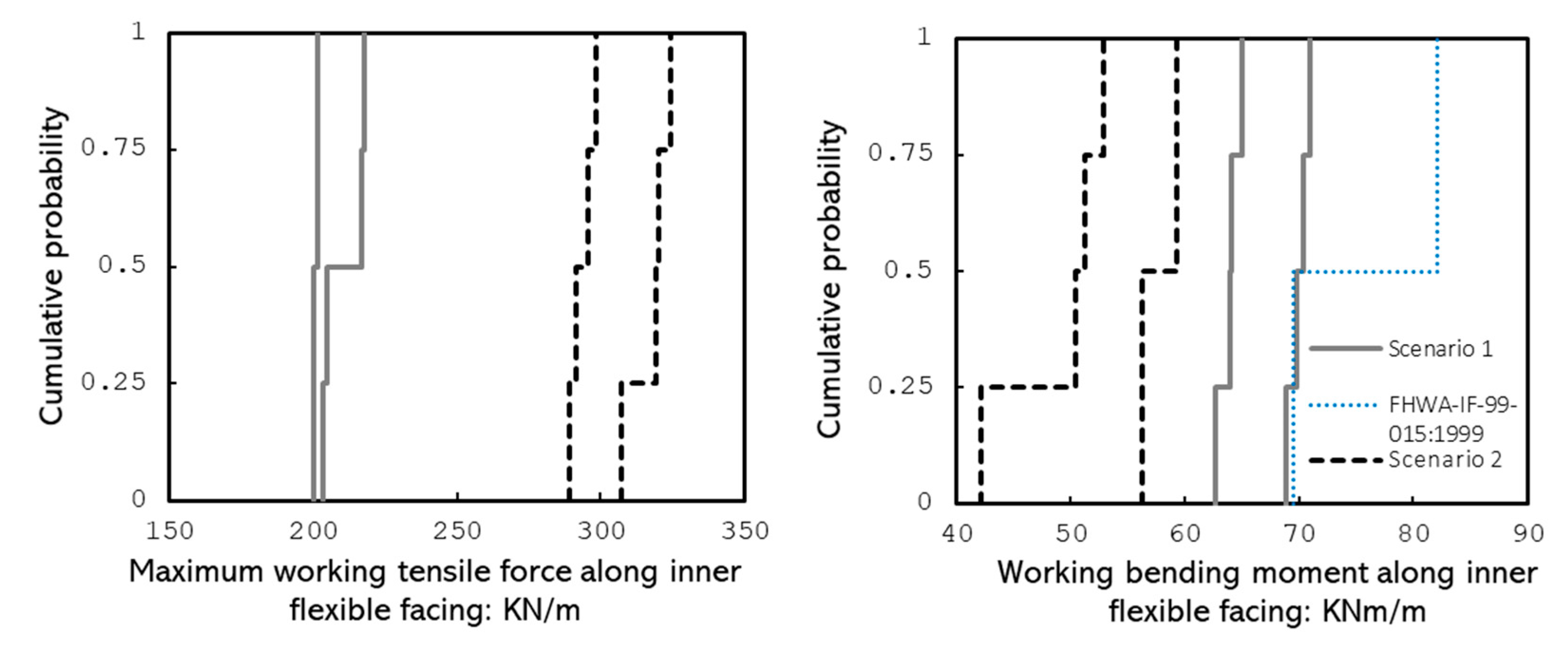
3.3.2. Bending Moments along Flexible Facing

To define the maximum bending moment along the shotcrete wall facing, the formulations offered for granular soils in the design code [21] for deep excavations were adopted and presented in Equations (6)–(11). For the soil fiction angle, ∅, the mean value for retained soils from the ground level to the bed of excavation was considered in the analysis. For standing groundwater, CIRIA [22] allows the use of the triangular water hydrostatic pressure envelope, with water pressure, U w , gaining value with the depth of the submerged soil, h w :
P [ k N / m 2 ] = 0.65 γ × H × K a
K a = tan ( 45 0.5 ) 2
U w = h w · γ w
w = 0.65 γ · H 2 · K a H 1 3   H 1   1 3   H n + 1
w = 0.65 γ · H 2 · K a +   γ w ( h w 2 3 H n + 1 ) H 1 3   H 1   1 3   H n + 1
M = w L 2 10
where M is the bending moment, w is the maximum uniformly distributed lateral load, H is the total height of the retained soil at the end of excavation, γ is the mean bulk density of the soil behind the wall, H 1 is the highest soil nail’s length of embedment, and H n + 1 is the distance between the lower-most nail and the bed of excavation. To find the value of the maximum bending moment, L can be substituted for the maximum vertical length of the nail influence area ( S v ) along the inner wall, in compliance with the recommendations of [23].

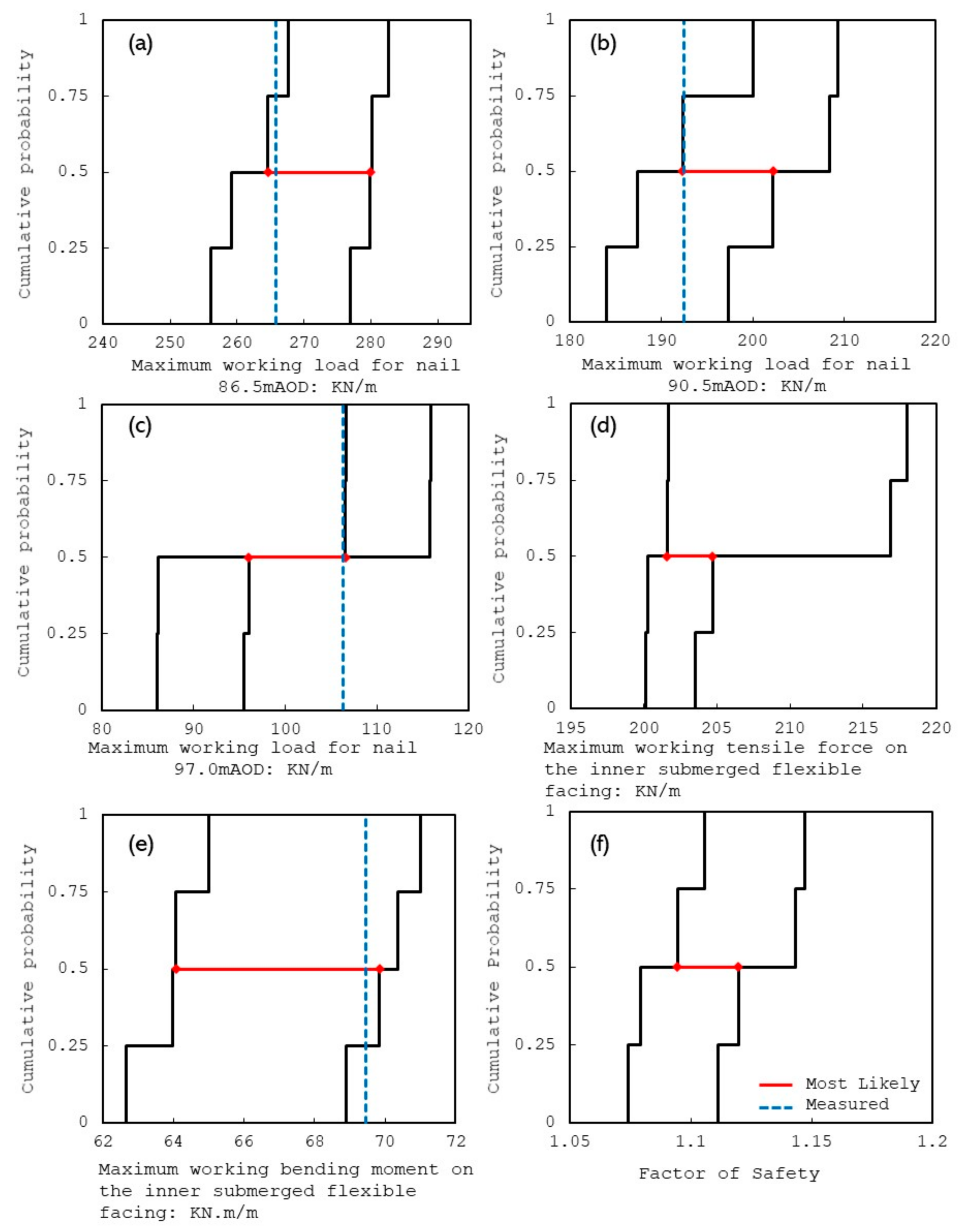
3.3.3. Axial Mobilized Force in Soil Nails

As per the recommendations of [5], soil nails were designed to carry the maximum possible axial force mobilized ( T m o b . ) at each elevation. The maximum mobilized axial force in soil nails was formulated using Equations (12) and (13) for the end of construction conditions and outer and inner walls, respectively. T m o b . excludes the effect of surcharge pressure at the ground level:
T m o b . = ( 0.65 0.75 ) γ · H · K a · S h · S v
T m o b . = ( 0.32 0.37 ) γ · H · K a · S h · S v
where γ is the soil unit weight, K a is the lateral pressure coefficient, S h is the horizontal spacing of nails, S v is the vertical spacing of nails, and S h × S v is the influenced area surrounding each nail. The mobilized axial force should be lower than the failure load (ultimate resistance), which can be determined for each reinforcement bar by multiplying the steel yield strength by the bar’s cross-sectional area. This is a conservative approach as steel bars sit within grouted drill holes.

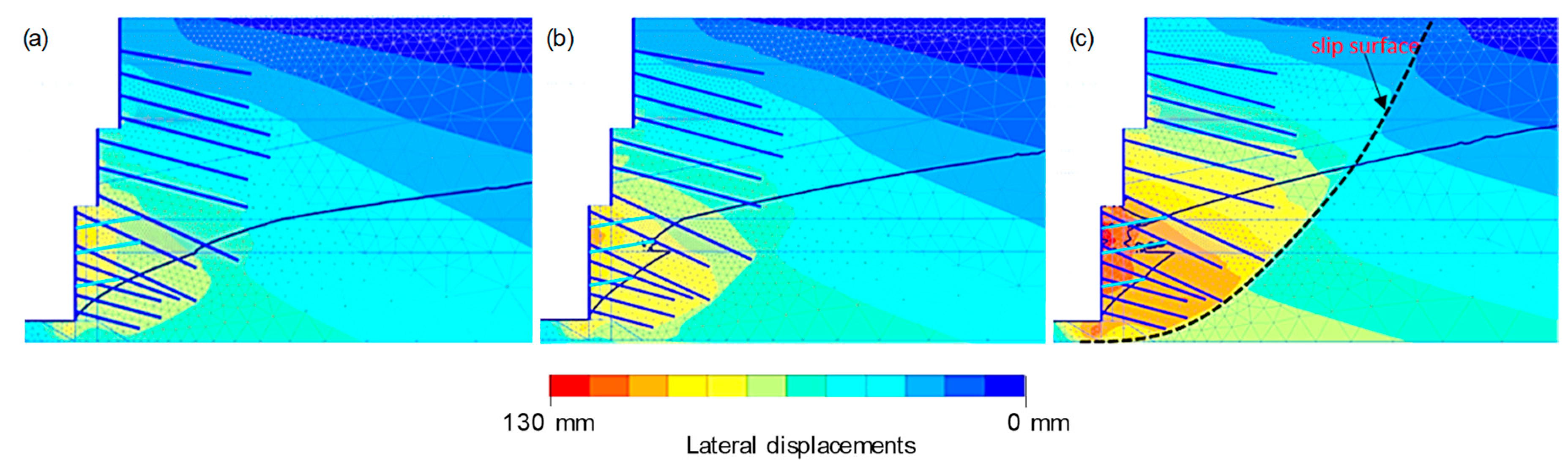
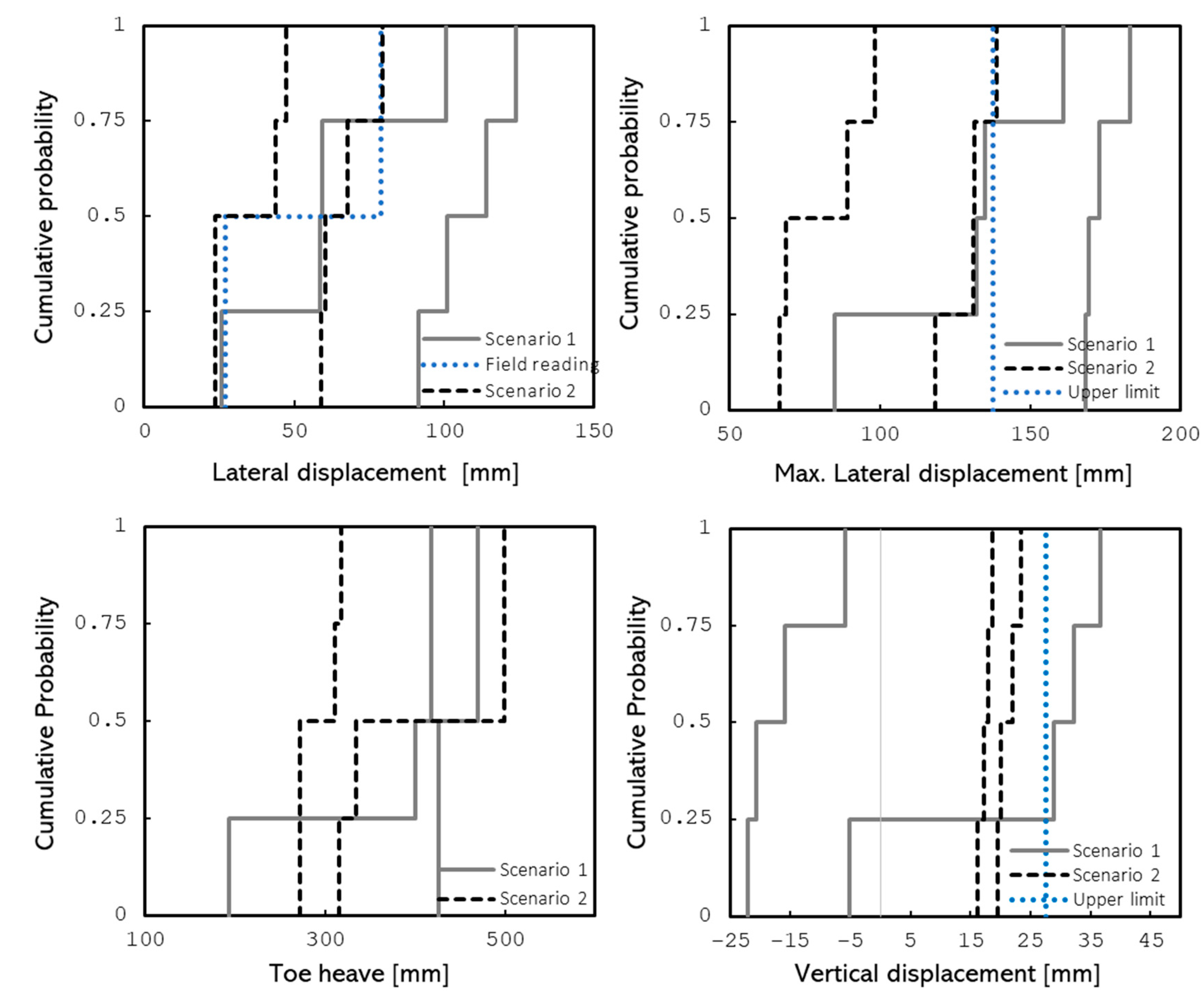
3.3.4. Lateral and Vertical Displacements

The actual lateral ground movements of the support system, originally designed using the mean factored material properties (Table 1) and actions, were measured in situ using laser deflectometers during and after construction. Survey data taken from nine reflectors installed at 97 mAOD and along the section of interest in this study were used as a benchmark for an assessment of the efficiency of the adopted probabilistic framework. The vertical displacement of the support system evaluated using the random set framework was contrasted with values from the analytical methods recommended in [21] code and in Equation (14):
δ ν = ( δ υ H ) i × H
where δ ν is the ground vertical movement, H is the total height of the retained soil, and ( δ υ H ) i is the coefficient of the soil properties.

4. Results

4.1. Design Scenario 1: Stochastically Dependent Variables

FHWA compliant calculated limit states are projected on belief and plausibility distribution functions [18] in Figure 3 for stochastically dependent cohesion and water level variables.
Limit states values pertinent to four realizations for each combination were sorted to derive the focal point extremes (i.e., minimum and maximum values). Middle values were discarded, and extremes were presented on the probability box in form of one step in the cumulative distribution function. As such, every step on the probability boxes represents extreme values for four random set combinations. Extreme values were sorted to form the upper and lower bound stepped line for each limit state. In Figure 3, the line marking the 0.5 cumulative probability represents the most likely values for each limit state, and the dashed line represents the index parameter either determined by the FHWA code of practice or measured in-situ. Lower and upper bounds are presented with stepped thick lines, with the space between representing possible values in the face of uncertain cohesion and water level. Table 4 summarises the design’s maximum axial force (Tmax) in soil nails 8 (submerged inner wall), 6 (middle wall), and 3 (outer wall) based on mean soil and water parameters. In Figure 4a–c, the design axial force for all walls falls within the probabilistically determined likely range and is relatively closer to the lower-bound line. This suggests that while the conventional design practice gives a reliable estimation of the soil nail axial force, variability of the water level can yield greater orders of axial loads, which is technically unexpected. While limit states are not reached and the system remains stable, the excessive axial forces in soil nails can impact the predicted ground lateral movements.
Using Equations (10) and (11), the mobilised bending moment on the critical submerged inner facing is 69.5 kNm·m−1, an order which is within the bounds of the upper and lower limit of the cumulative distribution function. It appears that the upper bound offers the most accurate estimation of mobilised moments, being consistent with the equivalent FHWA compliant index value (Figure 3e). Most likely the global factor of safety ranges between 1.094 to 1.120 (Figure 3f).
Figure 5 presents the p-box of the lateral and vertical displacement of the system in relevance with the measured lateral displacement at the end of construction and the design vertical displacement, taking the mean material properties and actions. The design’s vertical displacement and in-situ measured lateral displacements were within the bounds and within the most-likely values, which, in the case of vertical displacements, appears to be a broad range. As such, the random set framework does not appear to be as useful in determination of vertical displacements at ground level. This can be due to the poor choice of variables or small size of the ground investigation data sets [18].

4.2. Design Scenario 2: Stochastically Independent Variables

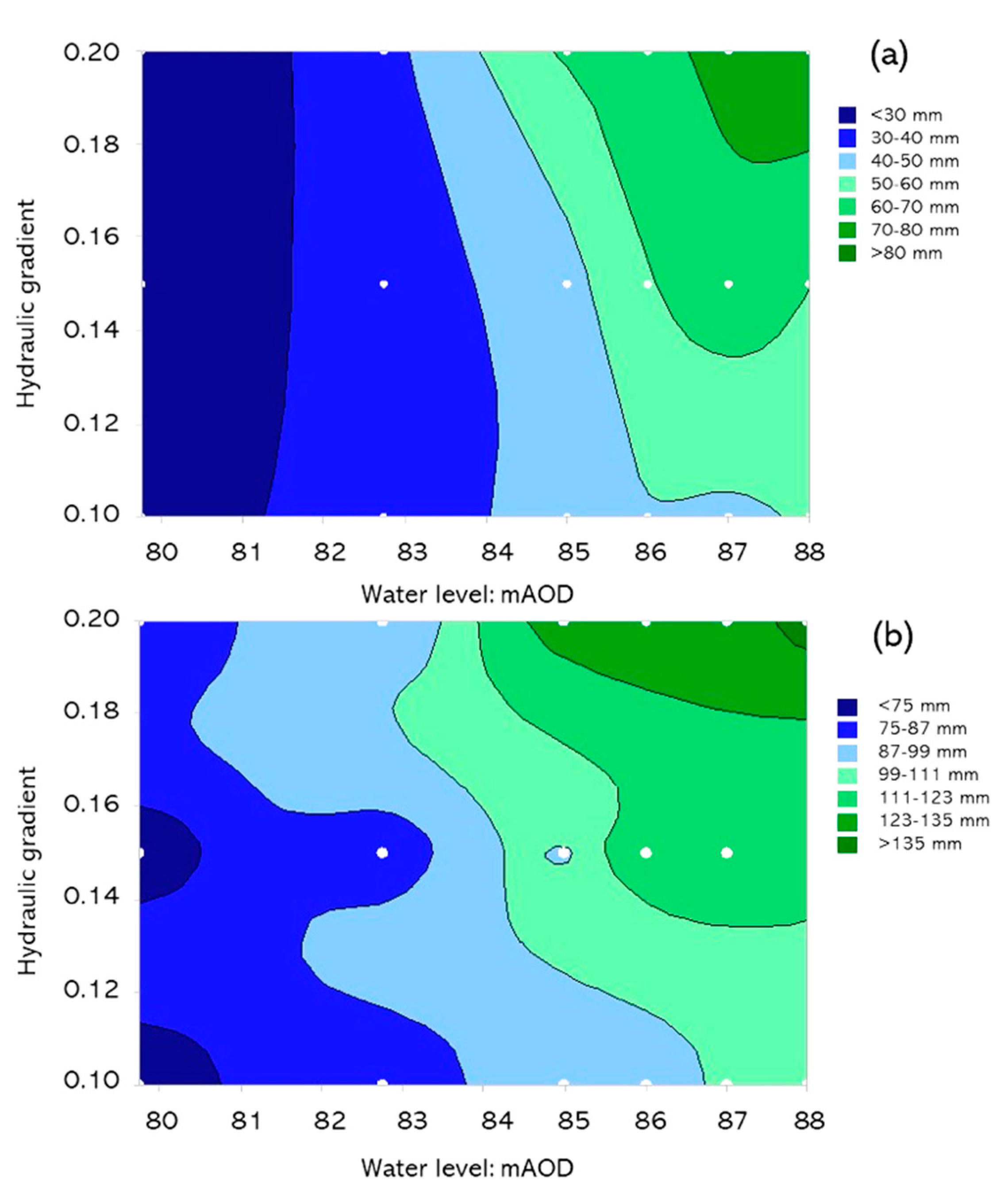
Implications of Seepage

Following seepage analysis (i.e., steady state flow analysis for end-of-construction stage) and for a low 0.1 hydraulic gradient and water level varying from 79.75 to 88 mAOD (scenario 2, set 1, lower-bound flow rate), it appears that the phreatic line passes from the toe of the excavation with a discharge rate of 0.018 to 0.037 m3/day/m, with no outflow through the drains. With an increase in the hydraulic gradient from 0.1 to 0.15 and 0.2, a re-distributed phreatic line appears to raise towards the drains, forming an outflow zone between the middle drain and the bed of the excavation (Figure 4). Discharge rates gained at drain points range between 0.018 to 0.037 m3/day/m. For a hydraulic gradient of 0.2, in particular, the re-distributed water table rose further to reach the upper drain, which is consistent with the imposed greater flow rates towards the drains. This is just above the design’s mean water level (under no seepage). The combined impact of flow through the inclined drains and change in geometry due to excavation led to alterations of the water level, causing drag and possible excessive hydrodynamic stresses. The equivalent enhanced hydraulic gradient appeared to be in the range of 0.16 to 0.19 (for pre-construction, original gradient of 0.15) and 0.22 to 0.24 (for pre-construction, original gradient of 0.2). This can have significant impacts on the lateral displacement of the retained wall. Figure 6 shows the impact on the lateral displacement at the reflect point (i.e., crest) and maximum lateral deflection of the water level and hydraulic gradient combined. The more pronounced impact of the hydraulic gradient as compared with the water level is obvious. Generally, the re-distributed water table is observed to strike the drains instead of the lining; this naturally yields lower pore water pressures immediately behind the facing, which is welcomed.
Limit states values pertinent to four realizations for each combination were sorted to derive the focal point extremes (i.e., the minimum and maximum values) and are presented in Figure 7 in the form of a series of probability boxes in the form of one step in a cumulative distribution function. Every step on the probability boxes represents extreme values for four random set combinations. Extreme values were sorted to form the upper and lower bound stepped line for each limit state.
The most likely global factor of safety ranges between 1.01 to 1.08 (as compared with design scenario 1, 1.094 to 1.120). The lower and upper bounds appear to offer a relatively wider range of most likely values, which is a welcomed event.
The FE predicted wall lateral deflection values for eight realisations ( u x R ) at the crest of excavation (i.e., the reflector point) are summarized in Table 5 for seepage conditions. In Table 5, z is the standardised normal variable, which represents the deviation of wall lateral deflections from the mean value, and subscripts LB, LQ, UB, and UQ denote the lower-bound, lower-quartile, upper-bound, and upper-quartile, respectively. Equation (15) formulates the z parameter:
z = u x R u x ¯ δ
where u x ¯ represents the mean deflection value and δ the standard variation, based on the FE-predicted and field actual values combined ( u x ¯ = 61.1   m m and σ = 16.5   m m ).
According to Table 5, realisations with the lowest z-values (arguably more realistic) represent combinations of the upper-bound head gradient with the lower-bound and lower-quartile water level, respectively. This suggests that [1]: When maximum hydraulic gradient occurs at a low water level (i.e., the dry season), the predicted serviceability is closest to the actual systems’ serviceability at the ground surface level, where lateral displacements should crucially fall within admissible limits to restrict any damage to neighbouring structures ( G L B , i U B in Table 5). Changing climatic conditions are generally believed to appear in the form of periods of intense rainfall over prolonged dry seasons; Ref [2] FE contour outputs suggest that drains are ineffective for the flow of groundwater under a lower-bound hydraulic gradient. This suggests that for piping to be mitigated, toe drains are required to be designed for lower-bound hydraulic gradient values. Drains, on the other hand, appeared to be fully functional for flow under upper-bound values of the hydraulic gradient. Drains are advisable to be designed for upper-bound hydraulic gradient values.
Figure 7 shows the probability distribution of post-construction serviceability of the system as a function of both stochastically dependent and independent variables.
Figure 8 illustrates the variation of the extreme values of the working normal force, together with the extreme values of the bending moment for the two modelling scenarios. The FE-predicted values can be contrasted with the computed values using the common FHWA code of practice.
Following the variation of the water level and possible mineral dissolution, the simplifications adopted in the conventional design practice appear to be admissible, as the calculated bending moment values match the upper-bound predicted values. In this, although the conventional design tends to neglect the effect of water level variation and possible impacts on soil strength, the resulting moment values are reasonably conservative.
For scenario 1, the below observations were made:
-
Lower-bound water level and upper-bound cohesion (representing dry season with maximum cementation) yielded the maximum factor of safety among the deterministic models.
-
Figure 8 shows the variation of the maximum bending moment on the inner wall (i.e., submerged) for the eight modelling scenarios. Solid lines represent the FE-predicted values, whereas the dashed line infers the designed mean bending moment according to the FHWA-IF-99-015 (1999) recommendations. Bending moment values derived from the FHWA formulation match those of the upper-bound RS values and as such are of reasonably good credibility.
For soil nails above the water level (at all times), the designed mobilised tensile forces’ (FHWA compliant) formulation closely matched those of the upper-quartile FE-predicted RS values. Where soil nails are located within the zone of water level variation, the design’s maximum tensile forces match the lower-bound values from the random set FE analysis. This shows the relatively small significance of the water level and cohesion variation in the determination of design actions of reinforcement nails.

5. Conclusions

A real-world deep excavation problem incorporating soil nailing was analysed and revisited, employing the random set finite element method to test the viability of the probabilistic frameworks in solving complex geotechnical problems, where spatial variability is prevalent. Two input data sets were established from a range of available ground investigation reports, and analysed together with field wall lateral displacement data that was captured over several months during and post-construction. The drained cohesion, hydraulic gradient, and water level were adopted as uncertain parameters for a critical cemented granular layer of soil stratum in the light of its susceptibility to mineral dissolution.
To study the impact of water level variation and subsequent alterations to the apparent cohesion of cemented soils (i.e., design scenario 1: stochastically dependent variables), random set realizations were defined using two datasets of equal probability. A further two input data sets were defined using stochastically independent hydraulic gradient and water level (i.e., design scenario 2) to revisit the stability and performance of the support system. For each scenario, four combinations were generated that contained 16 realisations; in other words, the infinite combinations of stochastically dependent and independent variables were reduced to 16 likely cases that were modelled using the FE Plaxis 2D code. The results obtained from the RS-FEM analysis were processed into cumulative distribution functions and then compared with design limit states (in compliance with the FHWA code of practice), and in-situ wall lateral displacement data taken from nine reflectors installed near the crest of excavation. The design limit state values were found to be generally consistent with the range of likely limit states offered by the RS-FEM framework and mostly lie within the most-likely range between the upper and lower bounds.
When considering the stochastic variables for the random field theory, careful reflection must be undertaken when making use of the hydraulic gradient as a critical variable, mostly due to the variables’ inability to predict material uncertainty. When considering the actions of the system, both the hydraulic gradient and cohesion variables produce a positive conclusion, which correlates well with the measured deflections and design limit states. A key positive of using cohesion as a stochastic variable is the insight that both the material and action responses match positively with the measured and observed results.
Retrieving good quality undisturbed samples to determine the shear strength of cemented granular soils continues to be a challenge. In a probabilistic framework, the tendency is to limit the uncertainty in the measurement of soil properties and to emphasise the variability of accurately measured soil properties; this is not plausible for the drained cohesion of cemented granular alluviums. A scope for replacing cohesion with a more reliably measurable alternative parameter is welcomed. This work outlines the benefits and limitations in using seepage and water level parameters as stochastically independent variables.

Author Contributions

Conceptualization, A.A.L and S.D; methodology A.A.L, S.G; software, J.W, K.T., M.M.,; validation, J.H; formal analysis J.W, K.T, M.M., A.L.L; investigation, S.G; resources, S.G and S.D; data curation, A.A.L; writing—original draft preparation, J.H; writing—review and editing, J.H and A.A.L.; supervision, A.A.L; project administration, A.A.L and S.D.

Funding

This research received no external funding.

Acknowledgments

Authors would like to thank POR Consulting Engineers and undergraduate research students in Newcastle University and University of East London for their technical inputs.

Conflicts of Interest

The authors declare no conflict of interest.

References

  1. UN. World Population Prospects: The 2012 Revision; UN Technical Report; UN: New York, NY, USA, 2013. [Google Scholar]
  2. The London Borough of Camden. Camden Planning Guidance CPG 4: Basements and Lightwells; The London Borough of Camden: London, UK, 2011.
  3. Assadi-Langroudi, A.; Theron, E. Gaps in particulate maters: Formation, mechanisms, implications. In Proceedings of the 17th African Regional Conference on Soil Mechanics and Geotechnical Engineering, Cape Town, South Africa, 7–9 October 2019; Geotechnical Division, South African Institute of Civil Engineers: Cape Town, South Africa, 2019. [Google Scholar]
  4. Assadi-Langroudi, A.; Jefferson, I. Constraints in using site-won calcareous clayey silt (loam) as fill materials. In XVI ECSMGE Geotechnical Engineering for Infrastructure and Development; ICE Institution of Civil Engineers Publishing: London, UK, 2015; pp. 1947–1952. [Google Scholar]
  5. Soil Nail Walls Reference Manual; FHWA-NHI-14-007; US Department of Transportation, Federal Highway Administration: Washington, DC, USA, 2015.
  6. Duncan, J.M. Factors of safety and reliability in geotechnical engineering. J. Geotech. Geoenviron. Eng. 2000, 126, 307–316. [Google Scholar] [CrossRef]
  7. Wong, F.S. First Order Second Moment Method. Comput. Struct. 1985, 20, 779–791. [Google Scholar] [CrossRef]
  8. Kunstmann, H.; Kinzelbach, W.; Siegfried, T. Conditional first order second moment method and its application to the quantification of uncertainty in groundwater modelling. Water Resour. Res. 2002, 38, 1–14. [Google Scholar] [CrossRef]
  9. Du, H.; He, W.; Sun, D.; Fang, Y.; Liu, H.; Zhang, X.; Cheng, Z. Monte Carlo simulation of magnetic properties of irregular Fe islands on Pb/Si(111) substrate based on the scanning tunneling microscopy image. Appl. Phys. Lett. 2010, 96, 1–3. [Google Scholar] [CrossRef]
  10. Griffiths, D.V.; Fenton, G.A. Three dimensional seepage through spatially random soil. J. Geotech. Geoenviron. Eng. 1997, 123, 153–160. [Google Scholar] [CrossRef]
  11. Goldsworthy, J.S.; Jaksa, M.B.; Fenton, G.A.; Griffiths, D.V.; Kaggwa, W.S.; Poulos, H.S. Measuring the risk of geotechnical site investigations. In Probabilistic Applications in Geotechnical Engineering; ASCE: Denver, CO, USA, 2007; pp. 1–12. [Google Scholar]
  12. Jiang, S.H.; Li, D.Q.; Cao, Z.J.; Zhou, C.B.; Phoon, K.K. Efficient system reliability analysis of slope stability in spatially variable soils using Monte Carlo simulation. J. Geotech. Geoenviron. Eng. 2014, 141, 1–13. [Google Scholar] [CrossRef]
  13. Tonon, F.; Mammino, A. A random set approach to the uncertainties in rock engineering and tunnel lining design. In Proceedings of the ISRM International Symposium on Prediction and Performance in Rock Mechanics and Rock Engineering (EUROCK ‘96), Torino, Italy, 2–5 September 1996; Volume 2, pp. 861–868. [Google Scholar]
  14. Tonon, F.; Bernardini, A.; Mammino, A. Determination of parameters range in rock engineering by means of Random Set Theory. Reliab. Eng. Syst. Saf. 2000, 70, 241–261. [Google Scholar] [CrossRef]
  15. Tonon, F.; Bernardini, A.; Mammino, A. Reliability analysis of rock mass response by means of Random Set Theory. Reliab. Eng. Syst. Saf. 2000, 70, 263–282. [Google Scholar] [CrossRef]
  16. Schweiger, H.F.; Peschl, G.M. Basic Concepts and Applications of Random Sets in Geotechnical Engineering. In CISM International Centre for Mechanical Sciences; Griffiths, D.V., Fenton, G.A., Eds.; Springer: Berlin/Heidelberg, Germany, 1975; Volume 491, pp. 113–126. [Google Scholar]
  17. Assadi, A.; Yasrobi, S.; Nasrollahi, N. A comparison between the lateral deformation monitoring data and the output of the FE predicting models of soil nail walls based on case study. In Proceedings of the 62th Canadian Geotechnical Conference and 10th Joint CGS/IAH-CNC Groundwater Conference, Halifax, NS, Canada, 20–24 September 2009. [Google Scholar]
  18. Nasekhian, A.; Schweiger, H.F. Random Set Finite Element method application to tunnelling. In Proceedings of the 4th International Workshop on Reliable Engineering Computing, Singapore, 3–5 March 2010. [Google Scholar]
  19. BS 8006-2:2011+A1:2017. Code of Practice for Strengthened/Reinforced Soils, Soil Nail Design; British Standards Institution: London, UK, 2011.
  20. Schikora, K.; Ostermeier, B. Two-dimensional calculation model in tunnelling verification by measurement results and by spatial calculation. In Proceedings of the 6th International Conference on Numerical Methods in Geomechanics, Innsbruck, Austria, 11–15 April 1988; Volume 3, pp. 1499–1530. [Google Scholar]
  21. US Department of Transportation, Federal Highway Administration. Geotechnical Engineering Circular No. 4: Ground Anchors and Anchored Systems; FHWA-IF-99-015; US Department of Transportation: Washington, DC, USA, 1999.
  22. Phear, A.; Dew, C.; Ozsoy, N.I.; Wharmby, N.J.; Judge, J.; Barley, A.D. Soil Nailing—Best Practice Guidance C637D; Construction Industry Research and Information Association CIRIA Publications: London, UK, 2005. [Google Scholar]
  23. BS 8002:1994. Code of Practice for Earth Retaining Structures; BSI: London, UK, 1994.
Figure 1. Cross-section diagram of the benchmark soil nailed system and adjoining features: SH is horizontal spacing, GL is ground level, PL is short for plate, mAOD is metres above ordnance datum, and Ø is diameter.
Infrastructures 04 00051 g001
Figure 2. Range of input variables in RS p-Box; scenario 1: Stochastically dependent variables: Water level and cohesion, scenario 2: Stochastically independent variables: Water level and flow rate.
Infrastructures 04 00051 g002
Figure 3. FHWA compliant limit states (index parameters) on RS p-Boxes and in relevance to the lower bound, upper bound, and most likely limit states in the face of uncertainty; (a) maximum mobilised working axial load in the eighth nail from ground level on the submerged inner wall, (b) maximum mobilised working axial load in the sixth nail from ground level on the middle wall, (c) maximum mobilised working axial load in the third nail from ground level on the upper wall, (d) maximum mobilised axial load along the inner submerged shotcrete facing, (e) maximum mobilised bending moment along the inner submerged shotcrete facing, and (f) global factor of safety.
Infrastructures 04 00051 g003
Figure 4. Re-distributed phreatic line following steady state flow and with relevance to drain points; input pre-excavation hydraulic gradients into the FE models: (a) i = 0.1, (b) i = 0.15, (c) i = 0.20.
Infrastructures 04 00051 g004
Figure 5. Serviceability limit state; post-construction (a) lateral displacements, (b) vertical displacement.
Infrastructures 04 00051 g005
Figure 6. Impact on the lateral displacement of the water level and hydraulic gradient; (a) displacement at the reflector level (97 mAOD, near crest), (b) maximum displacement.
Infrastructures 04 00051 g006
Figure 7. RSFEM modelling results on the p-Box; scenario 1: Stochastically dependent variables: water level and cohesion, scenario 2: Stochastically independent variables: water level and flow rate.
Infrastructures 04 00051 g007
Figure 8. Post-construction deterministic FE predicted mobilised actions on the inner lining: Scenario 1: Stochastically dependent variables: water level and cohesion, scenario 2: Stochastically independent variables: water level and flow rate.
Infrastructures 04 00051 g008
Table 1. Stratification and factored (i.e., design) engineering properties used in deterministic analysis.
LayerSoil TypeDepth: mΨ: °ϕ′: °C’: kPaγ: kN/m3E: kPaνKh: m/sKv: m/s
1Made Ground0.0–1.20120101798000.41.0 × 10−41.0 × 10⁻⁸
2Silty clayey sand1.2–4.21428201824,5000.31.2 × 10−41.2 × 10⁻⁸
3Alluvium4.2–9.21428251824,5000.353.1 × 10−43.1 × 10⁻⁸
4Silty clayey sand9.2–18.21434201834,3000.34.2 × 10−74.2 × 10⁻⁷
5Clay18.2–21.2025351934,3000.41.9 × 10−73.28 × 10⁻⁸
6Gravelly sandy clay21.2–29.21430251949,0000.31.31 × 10−74.36 × 10⁻⁶
7Silty clayey gravel29.2–35.01436201958,8000.33.6 × 10−91.0 × 10⁻⁹
Ψ = dilation angle, ϕ′ = drained friction angle, C’ = drained cohesion, γ = bulk unit weight, E = modulus of elasticity, ν = Poison’s ratio, Kh = horizontal coefficient of permeability, Kv = vertical coefficient of permeability.
Table 2. Material properties for flexible facing and soil nail elements.
MaterialEeq: kPaSh: mDdh: mEI: kN·m−2·m−1EA: kN·m−1Model
Nail elements (top nine rows)2.10 × 1082.500.081.38 × 1023.81 × 105Elastoplastic
Nail elements (lower four rows)2.10 × 1082.000.081.72 × 1024.79 × 105Elastoplastic
Reinforced shotcrete facing---2.50 × 1033.00 × 106Elastic
Eeq = equivalent modulus of elasticity for grouted soil nails, Sh = horizontal spacing, Ddh = diameter of drill holes, EI = bending stiffness, EA = normal or axial stiffness.
Table 3. Input random sets for two design scenarios.
DatasetC’: kPaWL: mAODI
Scenario 1Set 120~2479.75~86
Set 222~2685~88
Scenario 2Set 1 79.75~860.1~0.15
Set 2 85~880.15~0.2
C’ = drained cohesion, WL = water level (post excavation), I = hydraulic gradient, mAOD = metres above ordnance datum.
Table 4. Maximum normal force in the soil nail results.
Diameter: mmDistance from Crest: mHorizontal Spacing: mVertical Spacing: mMaximum Normal Force: kN/mFailure Load: kN/m
DHShSvTmaxTf
Nail 82821.52.52.25265.8255.4
Nail 63216.22.52192.46333.6
Nail 3329.682.52.5106.37333.6
Table 5. Lateral deflections from FE analysis: maximum values at reflector point.
G L B , i L B G L Q , i L B G U Q , i L B G U B , i L B G L B , i U B G L Q , i U B G U Q , i U B G U B , i U B
u x R : mm41.145.949.055.258.264.869.276.5
z –1.2–0.9–0.7–0.3–0.10.20.50.9
G = Water level, I = hydraulic gradient, LB = lower-bound, UB = upper-bound, LQ = lower quartile, UQ = upper quartile.

