Article

Shake Table Testing of Voltage and Current Transformers and Numerical Derivation of Corresponding Fragility Curves

1
European Centre for Training and Research in Earthquake Engineering (Eucentre), Via Ferrata 1, 27100 Pavia, Italy
2
Department of Civil Engineering and Architecture, University of Pavia, Via Ferrata 3, 27100 Pavia, Italy
3
Ricerca sul Sistema Energetico—RSE S.p.A., Via Rubattino 54, 20134 Milan, Italy
*
Author to whom correspondence should be addressed.
Submission received: 8 November 2022 / Revised: 4 December 2022 / Accepted: 5 December 2022 / Published: 14 December 2022
(This article belongs to the Special Issue Seismic Reliability Assessment and Advances in Structural Modelling)

Abstract

:
Damage to devices installed in electric substations, which have shown vulnerable behaviour under strong earthquakes in the last decades, may endanger power delivery in the emergency phases during and after an earthquake. Within seismic risk assessment of power networks, the definition of the fragility functions of electric equipment is paramount. However, in the current literature the availability of such fragility models for some specific electric substation components, including instrument transformers, is relatively limited, this being the reason behind the deployment of the current experimental and numerical research endeavour. Two voltage transformers and two current transformers having different system voltage levels (respectively in the high voltage HV and extra-high voltage EHV ranges) were subjected to shake table tests, and the experimental results were used to calibrate the corresponding 3D numerical models developed in OpenSees. A number of nonlinear dynamic analyses carried out within a multiple-stripe analysis (MSA) framework allowed the derivation of 16 fragility curves for the four transformers in both stand-alone and elevated/supported configurations, considering also two different soil types. Based on the derived curves, one of the voltage transformers is expected to experience light or negligible damage due to earthquake shaking, owing to its high resonance frequencies (and hence stiffness), whilst the remaining three devices may suffer moderate damage under medium to strong shaking intensities; however, their seismic risk is in effect mitigated by the presence of the typically employed supporting column. Comparison against models available in the literature lent valuable reassurance on the adequacy of the employed methodology and the reliability of the derived fragility curves.

1. Introduction

The evaluation of the safety level and the vulnerability of the electric power system under seismic events is based on the analysis of the dynamic behaviour of its structural and non-structural components. In particular, the latter, represented by various devices included within electric substations, have shown vulnerable behaviour under strong earthquakes in the last decades (Koliou et al., 2012) [1]. In fact, such components represent one of the most critical concerns when it comes to assessing the seismic reliability of a power transmission and distribution system, since they are among the major contributors to economic and functionality losses, thus endangering power delivery in the emergency phases during and after an earthquake. In an endeavour to evaluate seismic risk of power networks, the definition of fragility functions of electric equipment installed in the substations is crucial. A seismic fragility curve expresses the probability of reaching or exceeding a structural response limit state (e.g., light damage, severe damage, collapse) of a system of interest as a function of a measure of intensity of the seismic shaking. If used in combination with data on seismic hazard at the site, a fragility curve is an effective tool that allows the analyst to define possible damage scenarios, based on which it is then possible to plan risk mitigation measures.
Given the relevance of the seismic vulnerability of a power network, the current literature includes a number of publications dealing with numerical modelling of electric components, execution of experimental tests or reliability methods for the derivation of seismic fragility functions. The work by Zareei et al. (2016) [2] focusses on the evaluation of the vulnerability of a 400 kV power transformer (PTR), a critical component in an electric substation. The seismic behaviour of a PTR is discussed, highlighting that one of the most common causes of damage during seismic shaking is the porcelain bushing failure. A refined 3D finite element (FE) model of the PTR was developed and used to obtain its fragility curves through the multiple-stripe analysis (MSA) method. Subsequently, the same authors, Zareei et al. (2017) [3], analysed the seismic vulnerability of another critical component of electric substations, a 420 kV circuit breaker, whose most likely failure mode is the fracture of porcelain in severely stressed locations. Two intensity measures (IMs), namely peak ground acceleration (PGA) and peak ground velocity (PGV), were employed to reduce data dispersion and allow a multivariate fragility analysis. Another interesting contribution to this field was provided by Baghmisheh and Estekanchi (2019) [4], who retrieved fragility functions of four 400 kV devices, namely, surge arrester, current transformer, circuit breaker and disconnect switch, in both stand-alone and interconnected (through a bus slider—rigid bus assembly) configurations. The incremental dynamic analysis (IDA) method, adopting PGA as the IM, was applied on the 3D numerical models to produce the fragility curves. Mohammadpour and Hosseini (2017) [5], instead, investigated the dynamic behaviour of a 63 kV substation porcelain post insulator, which was subjected to shake table tests in two configurations, with and without its supporting truss structure. Based on the test results, the dynamic identification of the specimen and the calibration of its 3D finite element numerical model were performed. The fragility curves related to two limit states were derived. Gökçe et al. (2018) [6] investigated the failure modes of two specimens of a 550 kV porcelain post insulator, which were subjected to quasi-static tests; the experimental results were then used to calibrate a finite element model of one of the specimens. In a follow-up endeavour, Gökçe et al. (2019) [7] introduced a low-cost polyurethane seismic isolation device (PSID) at the base of the same 550 kV post insulator. Subsequently, Gökçe et al. (2021) [8] assessed the efficacy of two alternative designs of the PSID, to be installed under a 550 kV post insulator. Two simplified 3D numerical models consisting of elastic frame elements and nonlinear springs were developed and validated using shake table test results. The fragility curves of both the fixed-base and isolated systems, obtained through IDA, proved that the seismic isolation devices are highly effective in reducing the base moment of the porcelain insulator. Comprehensive system and component fragility curves, expressed as a function of two different IMs, namely PGA and peak acceleration response (PAR), were derived by Wen et al. (2019) [9] for two common types (230 kV and 550 kV) of disconnect switches in two operation configurations, using IDA and calibrating the developed FE models against static and dynamic test results. Fragility functions for a number of electric components can also be found in a database assembled by RSE (Gatti et al., 2002) [10], as well as in the database developed within the European project SYNER-G (2012) [11], which reports fragility functions coming from different sources, such as Vanzi (2000) [12] and HAZUS (FEMA, 2003) [13], among others. Finally, it is noted that valuable research work that however focussed solely on the numerical modelling or the execution of experimental tests on electric equipment, without the derivation of fragility curves, is described in the publications by Whittaker et al. (2004) [14], Koliou et al. (2012, 2013) [1,15], Moustafa and Mosalam (2016) [16], and Oliveto and Reinhorn (2018) [17].
For what concerns the specific case of fragility functions for high voltage instrument transformers, the information currently available in the literature is relatively scarce, for which reason the seismic response of two voltage transformers and two current transformers, designed for different system voltage levels (respectively in the high voltage HV and extra-high voltage EHV ranges), was herein experimentally and numerically investigated. The devices, provided by the manufacturer company Trench Italia S.r.l., were tested on one of the shake tables of the Eucentre Foundation (Pavia, Italy). Subsequently, 3D numerical models of the four transformers were developed in OpenSees (McKenna et al., 2000) [18] and calibrated against the results obtained from the shake table tests, in terms of resonance frequencies and dynamic responses. After defining the failure modes of interest, the corresponding limit states, as well as the demand parameters and their capacity values (i.e., damage thresholds), a number of nonlinear dynamic analyses were undertaken on such calibrated models within a MSA framework. A total of 16 fragility curves were derived, related to the four transformers in their stand-alone and elevated/supported configurations, considering also two different soil types (hence different sets of records). Valuable reassurance on the adequacy of the employed methodology and the reliability of the obtained curves was provided by the comparison with fragility models available in the literature for similar devices.
Section 2 describes in detail the specimens and the execution of the shake table tests, together with the dynamic identification process. The finite element models and their calibration against the experimental results are reported in Section 3 and Section 4, whilst Section 5 presents the methodology adopted in this work to obtain the seismic fragility curves of the investigated transformers. A number of aspects are addressed, including the choice of a structural reliability method (i.e., MSA), the record selection procedure, the definition of failure modes, limit states and demand parameters, as well as the execution of the nonlinear dynamic analyses on the developed numerical models. The conclusions are reported in Section 6.

2. Shake Table Tests

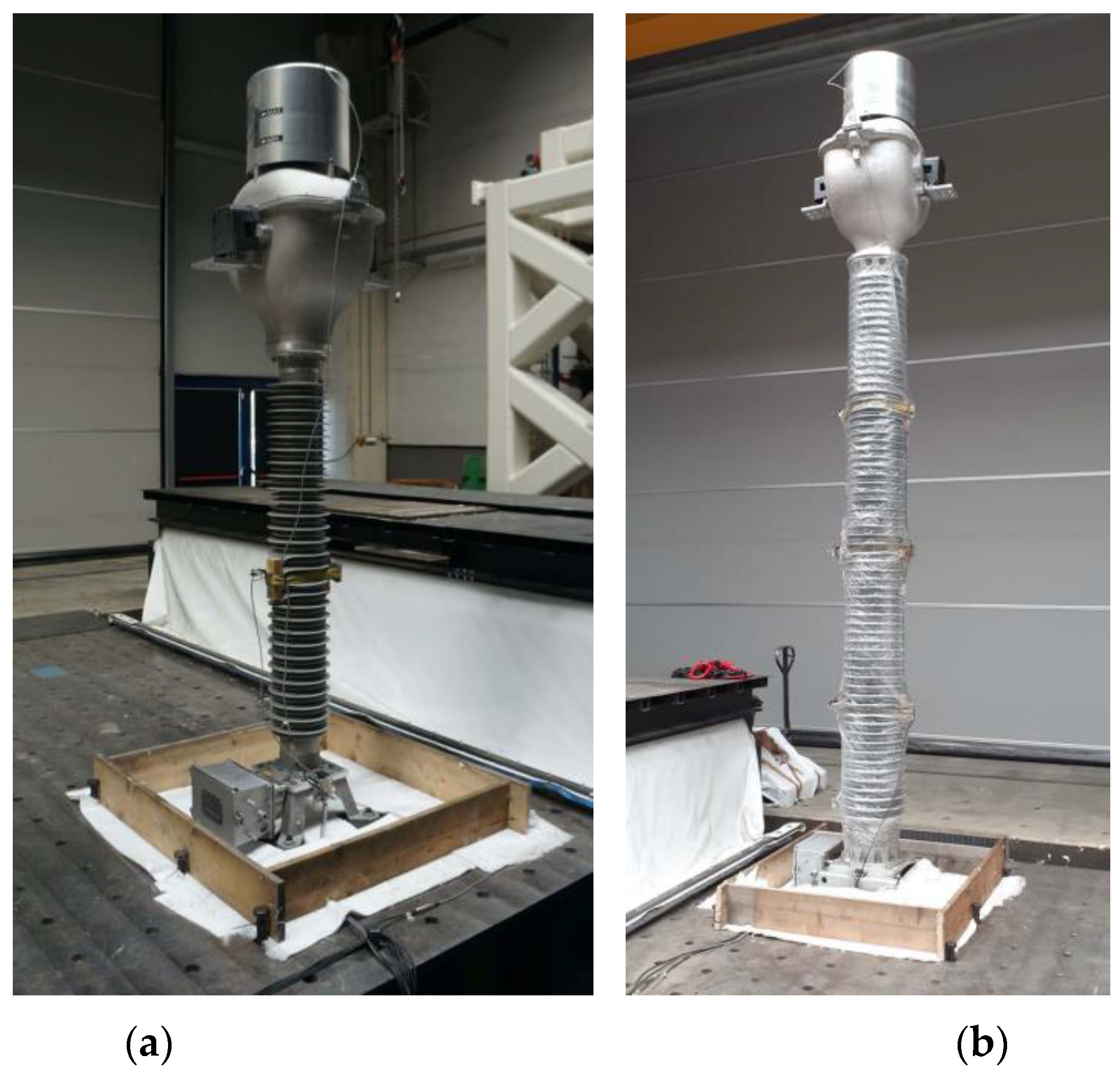
2.1. Specimens and Instrumentation

As already mentioned in the introduction, the specimens that were experimentally tested in this endeavour consisted of four full-scale instrument transformers designed for two different high voltage system levels (respectively in the high voltage HV and extra-high voltage EHV ranges); two of the devices are voltage transformers (VTs) and two are current transformers (CTs). Given that the six degrees of freedom shake table employed in this study is 4.8 m × 4.8 m in plan, it would have been possible to install and test all four specimens simultaneously. However, given the markedly different properties of the VTs with respect to the CTs, in terms of geometry, materials and dynamic properties (as will be shown in the next Section), it was decided to carry out the tests on two distinct (consecutive) days, the first of which was dedicated to the two voltage transformers, and the second one to the two current transformers.
The main technical specifications of the specimens, which hereafter are also called units under test (UUT, numbered from 1 to 4), are reported in Table 1, whilst Figure 1 and Figure 2 show individual photos of the four devices as mounted on the shake table. From the data in Table 1 and the images in Figure 1 and Figure 2, it can be noticed that, in each testing day, one “short” and one “tall” device were tested. The short and tall specimens were equipped with three and five accelerometers, respectively, numbered from #1 to #8 in Figure 3. The sensors are uniquely identified by their serial number; the sensor with SN 258331 (numbered as #9 in Figure 3) is always rigidly fastened to the table. A low-pass filter with 100 Hz cut-off frequency was applied to the signals recorded by all the accelerometers.

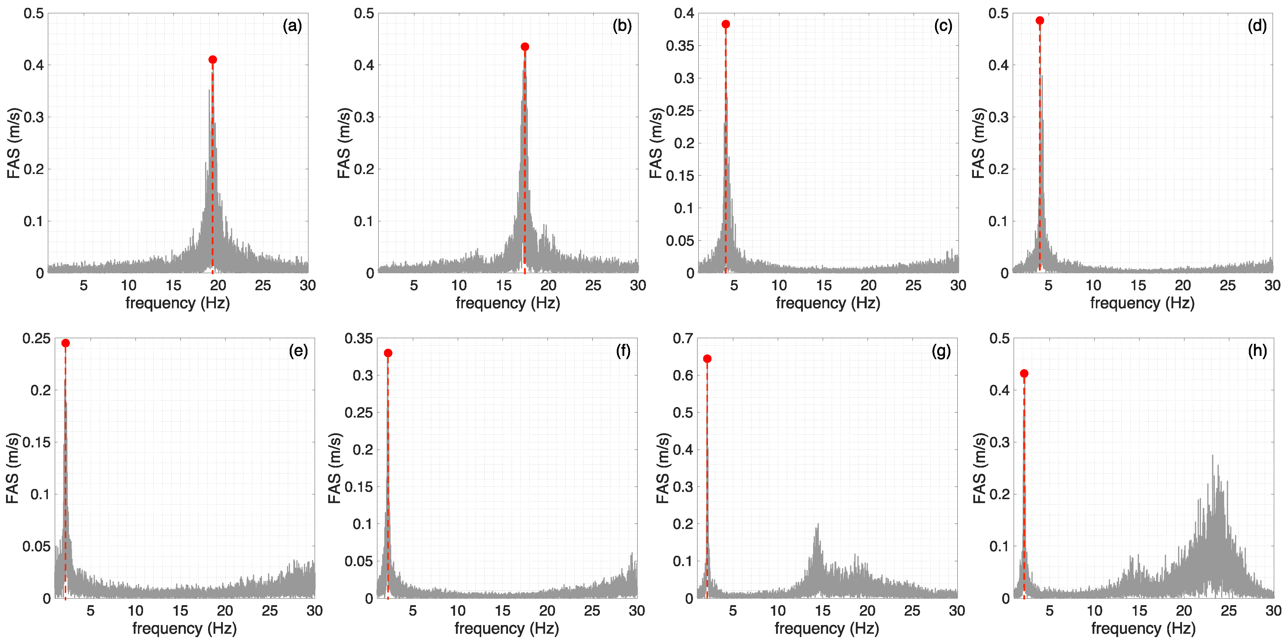
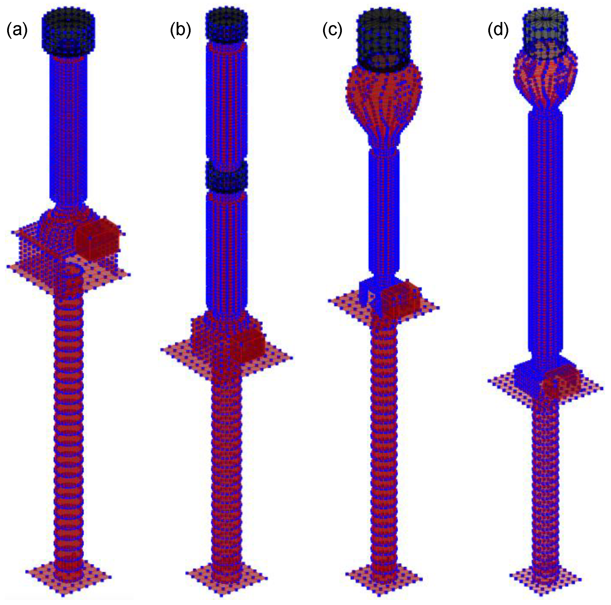
2.2. Dynamic Identification of Specimens

Dynamic identification tests (also known as resonance search tests) can be performed using different types of signals to characterise the UUT’s natural frequencies, namely, white noise, impulse, and sine sweep. The appropriate excitation signal is selected as a function of the characteristics of the UUT, on a case-by-case basis—in the current endeavour, the application of a white noise signal was adopted.
At the beginning and at the end of each of the two testing days, as well as during the execution of the seismic simulation tests (see next Section), several random white noise runs were conducted, separately along each of the three axes, to allow for the dynamic identification of the specimens and to monitor possible changes of the natural frequencies, which would indicate the presence of structural damage. The signals obtained from the accelerometers #1 and #4 (see sensor numbering in Figure 3), installed at the top of the two specimens in both testing days, were selected as the output responses of interest for the computation of the Fourier amplitude spectrum (FAS). Figure 4 shows the peaks (red dots), representing the resonance frequencies of all four specimens, picked on the FAS functions in both the X- and Y-directions, in the intact configuration (i.e., at the beginning of the two testing days); the corresponding numerical values are reported in Table 2, where it can be noticed that the two identified frequencies are quite similar for UUT1 and coincident for the remaining three specimens.
From the FAS plots in Figure 4 it is possible to observe the absence of higher dominant peaks in the output signals. Only for UUT4, i.e., the CT H3-34794, several additional peaks are visible up to 30 Hz; however, such peaks are deemed to be caused by high-frequency numerical noise in the signals, the latter being not filtered for the dynamic identification phase. Based on these observations, all four transformers can be considered as single-degree-of-freedom (SDOF) systems, characterised by a sole resonance (and fundamental) frequency, or equivalently, as being three-dimensional systems, by two resonance frequencies, which are similar or coincident, one per horizontal direction.
The dynamic identification of the specimens carried out at the end of each of the two testing days to capture possible changes of the natural frequencies that could reflect the presence of damage, yielded the resonance frequencies reported in Table 3. It can be readily observed how these frequencies are slightly lower than the ones at the initial intact stage only for UUT1, suggesting that the latter may have experienced light damage (an alternative cause could be a potential loosening of the bolts fastening the specimens to the shake table during the execution of the seismic simulation tests—see subsequent Section). For the remaining three specimens, on the other hand, the frequencies were essentially unchanged.

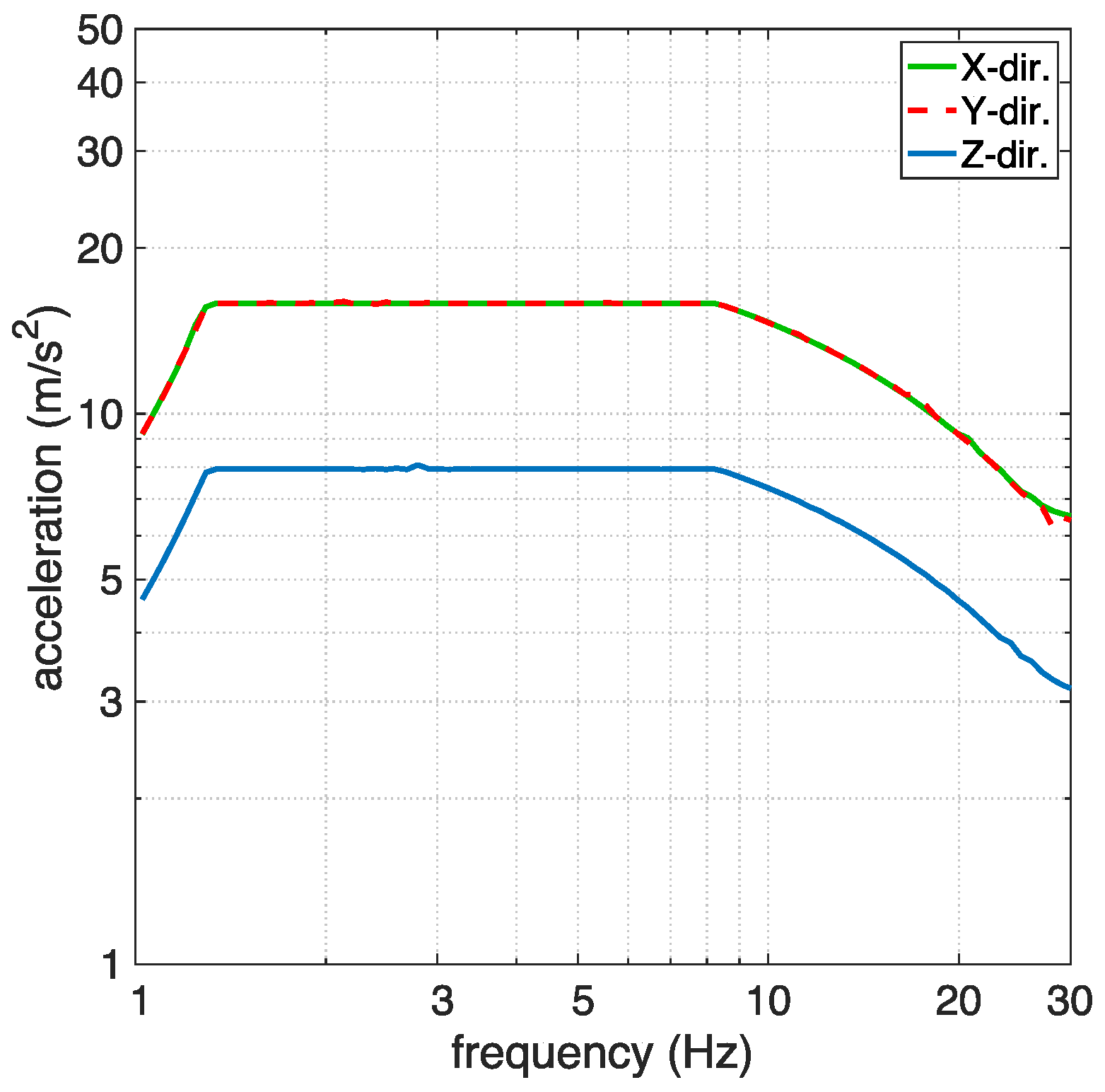
2.3. Seismic Simulation Tests

The seismic simulation tests performed were designed to conform to the required response spectrum (RRS) specified by ICC-ES AC156 (2015) [19]. All tests were conducted simultaneously in the longitudinal, transversal, and vertical displacement degrees of freedom (DOFs), with each DOF excited by an independently generated table motion profile. Figure 5 shows the RRS for horizontal and vertical acceleration adopted in the tests, for the considered test level; it is noted that the employed target spectra along the X- and Y-directions were actually slightly different, so as to produce non identical signals in the two directions. The signals used for the test of the UUTs were generated according to ICC-ES AC156 (2015) [19] using an iterative spectrum-matching procedure. A damping ratio of 5% and a frequency resolution of 24 lines per octave were used to generate the signals. A 30 s time-history shaping function, consisting of 5 s rise time, 20 s of sustained (strong) motion, and 5 s of decay, was used to shape the table motion amplitude in the time domain. Independent and uncorrelated records were generated for each orthogonal degree of freedom, considering also scaling levels ranging from 20% to 115% of the target RRS, so that the tests could be executed through the application of a sequence of input signals of gradually increasing intensity; the complete test sequences, as well as more detailed information on the employed testing protocol, can be found in the report by Eucentre (2021) [20] and the paper by Cavalieri et al. (2022) [21]. After the tests, the specimens did not show any visible damage or significant deformation.

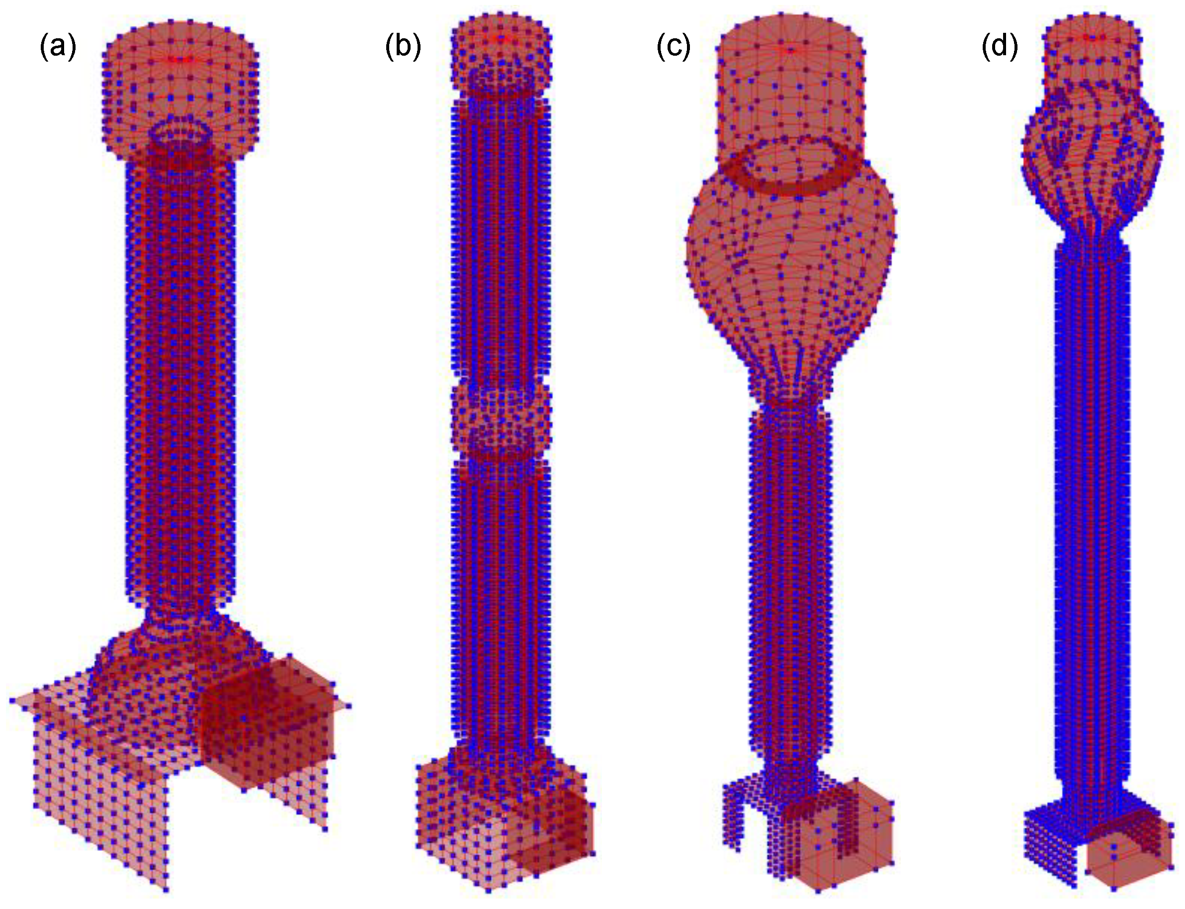
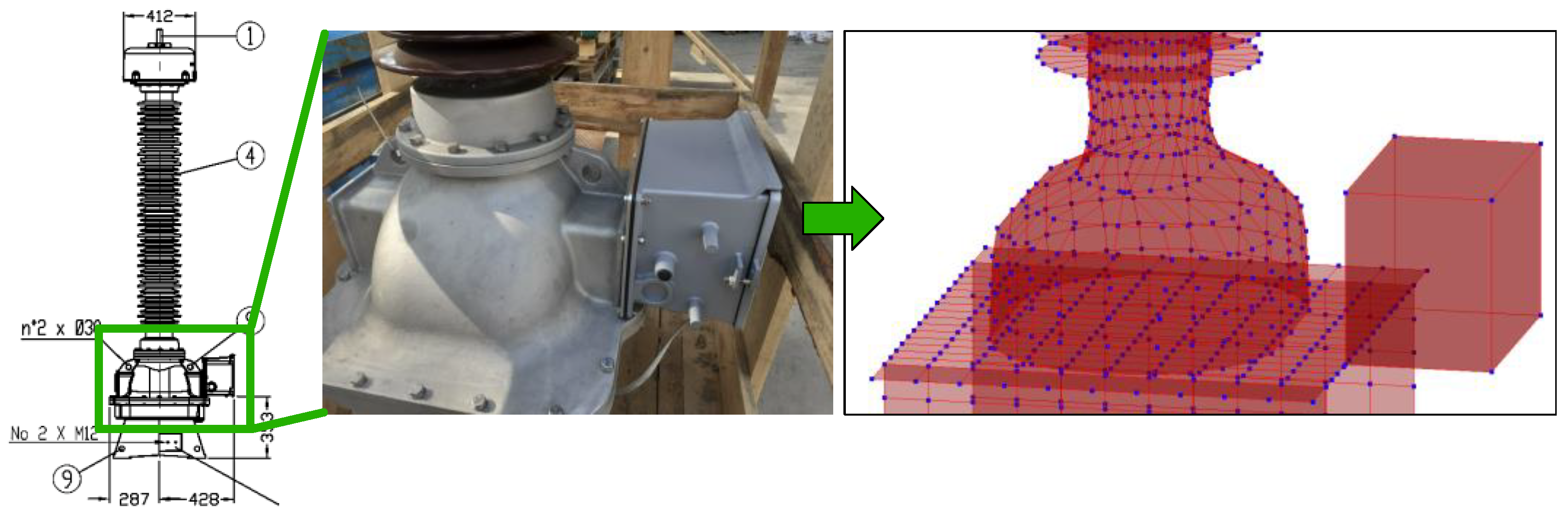
3. FE Numerical Modelling of the Transformers

Three-dimensional numerical models of the four transformers were developed in the open-source finite element software OpenSees [18]. Given the geometric complexity of the models at hand, it was also decided to make use of the freely available graphical user interface of OpenSees, namely OpenSees Navigator (Yang and Schellenberg, 2004) [22], for this work downloaded in the form of a MATLAB P-code, allowing for the parametric generation of the complete OpenSees model as a .mat variable within MATLAB (The MathWorks, 2019) [23]. The main geometric properties of the four models were defined on the basis of the drawings provided by the manufacturer and the visual inspection of the specimens. The adopted modelling strategy consisted in simplifying the complex geometry (e.g., the shape of several surfaces) of the transformers and reproducing the main portions of the external structure. Concerning the voltage transformers (VTs), whose models are shown in Figure 6a,b, the main components that were explicitly modelled are the following:
  • Vertical supports of the base plate;
  • Metallic base plate;
  • Base of the ceramic/porcelain insulator bushing;
  • Hollow ceramic/porcelain insulator bushing;
  • Metallic hollow top cylinder;
  • Secondary terminal box.
The base of the ceramic bushing differs in the two VTs: in model H3-40469 (HV range) it has the shape of a metallic spherical cap, whilst in model H3-36523 (EHV range) it is a raised portion with a pseudo-cylindrical shape. Furthermore, model H3-36523 is also taller and characterised by the presence of two bushings and two metallic top cylinders, instead of just one.
With regards to the current transformers (CTs), whose models are shown in Figure 6c,d, the main components that were modelled are the following:
  • Vertical supports of the base plate;
  • Metallic base plate;
  • Hollow insulator bushing;
  • Metallic head;
  • Metallic hollow top cylinder;
  • Secondary terminal box.
Both devices have only one bushing, which is however taller and squattier in model H3-34794 (EHV range). The modelling of all thin-wall portions was implemented using four-node shell elements (ShellMITC4 in OpenSees). In the models of the stand-alone transformers (i.e., without a supporting column), the base nodes of the vertical supports were rigidly fixed to the ground by restraining them in all six directions. Moreover, master-slave constraints (equalDOF in OpenSees) were applied to nodes in the contact zones between the terminal box and the base plate or supports (depending on the model), between the base of the bushing and the base plate (in the VTs models), between the bushing and the base plate (in the CTs models), and between the base plate and the supports (in model H3-35245).
In the drawings made available by the manufacturer, there are no details about the materials and their properties, as well as several dimensional properties such as the thickness of the components. For this reason, the material types and the values of several properties used in the modelling were assumed based on expert judgement, visual inspection, and information available in the literature, and then adjusted during the phase of model calibration against the experimental results. The main characteristics of the materials adopted in the models are reported below.
Regarding the materials composing the external structure of the models, the major distinction is related to the bushings, which are composed of a hollow central cylinder and external sheds on the perimeter to ensure adequate surface insulation behaviour under external pollution conditions, equally spaced along the height. In the two VTs, both the cylinder and the sheds are made of ceramic material, identified as aluminous porcelain C-120 (according to standard IEC 60672-3); in the models, the shell elements representing these ceramic components were assigned a linear elastic section (ElasticMembranePlateSection in OpenSees), with Young’s modulus E = 8.0 × 10⁴ MPa and Poisson’s ratio n = 0.17. On the other hand, in the two CTs, the bushing is composed of a hollow stiff internal cylinder, made of GFRP (fiberglass) coated externally with high temperature vulcanized (HTV) silicone rubber, the latter being also the material constituting the sheds. The corresponding shell elements were assigned linear elastic sections, with E = 1.5e04 MPa and n = 0.25 for GFRP, and E = 2.25 MPa and n = 0.48 for HTV. The terminal boxes and the top cylinder of all models are made of a material that was identified as aluminum, assumed to be elastic with E = 7.0 × 10⁴ MPa and n = 0.33, whilst the remaining external portions are made of steel, the only material considered as nonlinear herein. In order to model the structural steel with nonlinear behaviour, a fibre section was defined (PlateFiber in OpenSees), which was then assigned the material Updated Voce-Chaboche (UVCmultiaxial in OpenSees). Its behaviour is described by a number of parameters, whose experimentally calibrated values are available on the OpenSeesWiki website [24] for different structural steels; two UVC models were selected among the ones reported in OpenSeesWiki, namely:
  • For the two VTs: UVC steel model S355J2 + N, with E = 197.41 GPa and yield stress fy = 338.80 MPa;
  • For the two CTs: UVC steel model S690QL, with E = 188.63 GPa and yield stress fy = 685.39 MPa.
For the complete set of input property values, including the adopted thickness of the components, interested readers are referred to the report by Eucentre (2021) [20]. A portion of the provided drawing related to transformer H3-40469, with a photo and the correspondent numerical model of one detail are shown in Figure 7.

3.1. Masses, Loads and Damping

In all OpenSees models, the allocation of the mass, variable along the height, was assumed on the basis of the transformers’ typology and their materials (of different mass densities), and then adjusted during the phase of model calibration against the experimental results. In the VT H3-40469, which can be considered as a “tank type” transformer, a high mass percentage was assigned to the lower part of the corresponding model. On the other hand, the two CTs can be considered as “head type” transformers: this is the reason why a high mass percentage was assigned to the upper part of the models, which encompasses not only the metallic head but also the top cylinder, the latter accommodating steel expansion compensators. Concerning the VT H3-36523, the mass in the model was distributed not based on the height, but rather by taking into account the different material mass densities and sizes of the transformer components, mainly distinguishing between the steel portions, namely, the supports, the base plate, and the two top cylinders, characterised by higher mass percentage, and the remaining portions, made of porcelain and aluminum.
Concerning the model loading, the gravity loads were applied as nodal loads. The total weight of each model was subdivided in at least two sets of nodal loads, with uniform distribution among the nodes for each set, to be applied at two different heights, in the upper and lower portions of the model, based on the mass distribution. The dynamic loads introduced for the execution of the nonlinear dynamic analyses were applied in terms of acceleration time-histories at the restrained base nodes. In the calibration phase against the experimental results, for each seismic simulation run (with target spectrum signal) a nonlinear dynamic analysis was executed on the generic model considering two input base acceleration signals, for the two horizontal directions (X and Y), taken from the experimental data. On the other hand, in the subsequent phase of seismic fragility analysis through the MSA method, in the nonlinear dynamic analyses only one input acceleration component was applied, along the more flexible direction of each model.
Concerning the damping settings for the dynamic analyses, a Rayleigh viscous damping formulation was employed in the models. In particular, a damping proportional to mass and tangent stiffness was adopted, and the two coefficients were computed considering the first two model frequencies (translational along X and Y) as control frequencies. The damping ratio values, calibrated on the base of the amplitudes of the experimental acceleration and displacement responses obtained in the seismic simulation tests, resulted to be 1%, 2%, 0.9% and 0.7%, for the H3-40469, H3-36523, H3-35245 and H3-34794 models, respectively.

3.2. Modelling of the Supporting Column

Typically, high voltage instrument transformers used in electric substations are not placed directly on the ground, but are rather mounted onto the top plate of a supporting structure (e.g., a truss, see Mohammadpour and Hosseini, 2017 [5]), which is used to bring the top of the device to the height necessary to attach the conductor cables. In order to reproduce these actual installation conditions, four transformer models including a supporting column were also created, whilst the conductor cables were not modelled, since they are usually flexible and therefore not deemed to influence in any significant fashion the dynamic response of the models.
Two different supporting columns were introduced, one for the 170 kV models (i.e., the short ones, H3-40469 and H3-35245) and another for the 420 kV models (i.e., the tall ones, H3-36523 and H3-34794), whose original drawings can be found in the report by Eucentre (2021) [20]. Both supporting structures are composed of a steel hollow cylinder, 4 mm thick, linked to upper and lower steel plates, 14 mm thick, by steel angles. The steel type is Fe 430 B. The columns for the 170 kV and 420 kV models are 2.85 m and 2.50 m tall and have a mass of 163 kg and 263 kg, respectively.
The steel angles were not modelled and both upper and lower plates were assumed to have a squared shape, for convenience. For consistency with the transformer models, the supporting column (intended as the cylinder plus the two plates) was modelled with shell elements, of course not including the sheds on the cylinder’s perimeter, and following the same automatic and parametric modelling strategy adopted for the transformers, as shown in Figure 8. EqualDOF constraints were applied between each of the upper nodes of the cylinder and their closest nodes belonging to the upper plate, whilst rigid links of type elasticBeamColumn were introduced between each of the lower nodes of the cylinder and their closest nodes belonging to the restrained ground plate. All shell elements of the column were assigned the same fibre section used for the transformer models. The total mass and weight of the supporting column were uniformly distributed among the nodes of the cylinder and the upper plate. The applied damping settings are the same as those used for the models without the supporting column, described above.

4. Calibration of the Numerical Models

The experimental results obtained from the shake table tests were used to calibrate the developed 3D numerical models of the four transformers in their configuration without the supporting column, which is the same configuration adopted for the tests. The values for the model parameters reported in the previous Section are the final ones assigned to the models after the calibration phase. The latter was undertaken in terms of (i) resonance frequencies and (ii) dynamic responses, namely, acceleration and displacement histories (recorded at the top of the specimens), as well as FAS of acceleration signals. The frequency-based model calibration was carried out against the resonance frequencies experimentally identified at the initial intact stage (i.e., at the beginning of each of the two testing days), whilst the response-based calibration was executed using the experimental results obtained at both the initial (lower intensity) and final (higher intensity) stages of the tests.

4.1. Calibration in Terms of Resonant Frequencies

For each of the four models, the calibration in terms of resonance frequencies was based on the comparison between the first two experimental frequencies, obtained through dynamic identification (at the initial intact stage), and the corresponding numerical ones, retrieved in OpenSees. Table 4 reports, for all four devices, the experimentally derived frequencies (the same already reported in Table 2) and the numerical eigenfrequencies of the calibrated models. As can be readily noticed, an excellent agreement was reached in terms of resonance frequencies. The eigenvalue analysis carried out on the models confirmed that the first two frequencies belong to translational modes in the X- and Y-directions.
Given the absence (or very limited relevance) of experimental higher modes for all devices, as also confirmed by the good agreement with the experimental dynamic responses, governed by the first two frequencies alone, as shown in the next subsection, it can be concluded that all four calibrated numerical models, like the physical devices, can be treated as SDOF systems, characterised by two resonance frequencies only, which are similar or coincident, one per horizontal direction. The first two modes are translational along the X- and Y-directions, and characterised by cantilever mode shapes, typical of a SDOF system.
For the sake of completeness, Table 5 reports, for all four devices, the first two eigenfrequencies of the calibrated models equipped with the supporting column. As expected, a reduction of the frequencies is observed with respect to the models without the column; such a reduction is relatively limited for all models except for the TV H3-40469, for which it is around 14 Hz and 13 Hz along X and Y, respectively, this model being much stiffer than the supporting column.

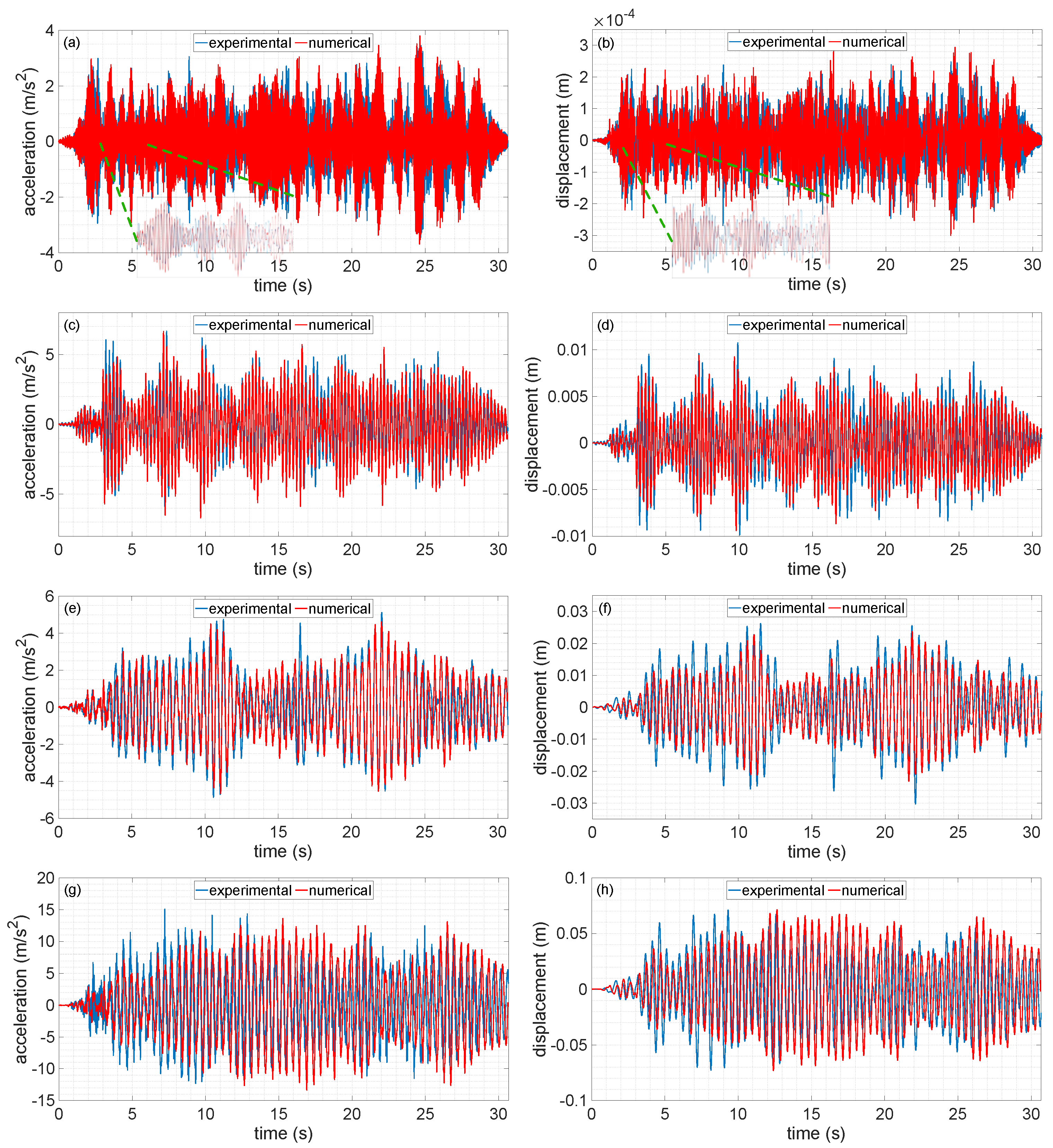
4.2. Calibration in Terms of Dynamic Responses

As mentioned above, the second calibration phase concerned the comparison between the experimental and numerical dynamic responses, in terms of acceleration and displacement histories recorded at the top of the specimens, as well as the FAS of acceleration signals. The experimental output responses in acceleration were obtained from the accelerometers #1 and #4 (see sensor numbering in Figure 3), installed at the top of the two specimens in both testing days, as done in the dynamic identification phase, whilst the numerical acceleration and displacement responses in both the X- and Y-directions were recorded (through OpenSees recorders within the nonlinear dynamic analyses) in the central node of the metallic top cylinder’s upper face.
The response-based calibration was carried out using the seismic simulation runs not only at the initial lower intensity stage, but also at the final higher intensity stage, with the aim to obtain validated numerical models that should be able to accurately reproduce the transformers’ behaviour at different increasing levels of seismic shaking. The latter cause the dynamic response of the models to evolve in a wide range, from the elastic field to possible excursions in the inelastic field, due to the nonlinear behaviour of the steel. This wide spectrum validation is paramount for the subsequent seismic fragility analysis (see subsequent Section), where these models will be subjected to high levels of earthquake excitation within the nonlinear dynamic analyses.
Before comparing the dynamic responses, filtering was applied to the signals, in the form of a fourth order Butterworth bandpass filter centred around the resonance frequencies, and therefore with lower and upper cut-off frequencies different for each device. The application of this filter also allowed retrieving accurate experimental displacement histories via double numerical integration of the acceleration signals, as well as clean plots of FAS of the latter.
Due to space constraints, Figure 9 shows the experimental–numerical comparisons of only acceleration and displacement histories, only along the X-direction and only for the seismic simulation runs at the initial lower intensity stage. It can be readily observed that for all models the experimental and numerical histories, both in acceleration and displacement, are correctly in phase between them, as expected given the agreement of the resonance frequencies. Since the frequencies at the end of each testing day were essentially unchanged for three specimens, and slightly lower than the ones at the initial intact stage only for UUT1, as seen above, the numerical histories were substantially in phase with the experimental ones also for the seismic simulation runs at the final higher intensity stage (not shown here). Concerning the signal amplitudes, overall the quality of the match in terms of both acceleration and displacement is quite good at the lower intensity stage, as can be observed in Figure 9 with reference to the X-direction; a similar quality was observed in the plots for the Y-direction. On the other hand, at the higher intensity stage (not shown here) the agreement is worse, while remaining acceptable; a potential reason for this could be a possible discrepancy between the experimental and numerical steel yield stress, something that under higher intensity excitations can naturally lead the top accelerations or displacements in the model to diverge from the corresponding quantities recorded during the tests.

5. Seismic Fragility Analysis

This final Section presents the methodology adopted in this work to obtain the seismic fragility curves of the investigated instrument transformers, from the choice of a structural reliability method, including the record selection procedure, to the definition of failure modes, limit states and demand parameters, up to the execution of the nonlinear dynamic analyses on the calibrated numerical models.

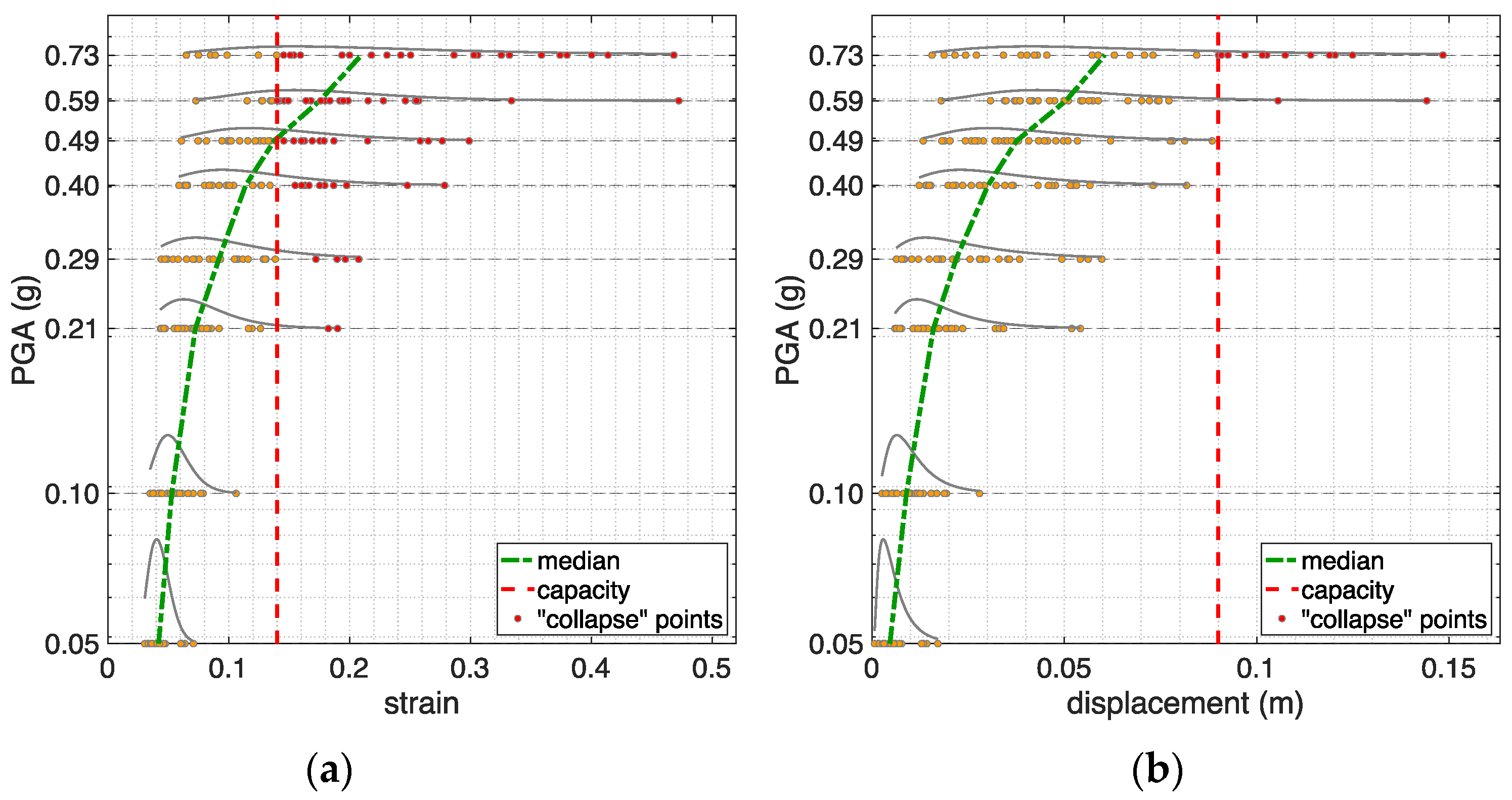
5.1. Multiple-Stripe Analysis (MSA)

A number of methods to develop fragility functions are available in the literature, many of which call for the undertaking of multiple nonlinear dynamic analyses (NDAs). MSA (Jalayer and Cornell, 2009) [25] and IDA (Vamvatsikos and Cornell, 2002) [26], which are both IM-based methods, rely on scaled motions and a relatively high number of NDAs. MSA was herein adopted, given its generally more efficient nature (Baker, 2015) [27]. Within MSA, multiple levels of intensity (i.e., the stripes, each corresponding to a return period) of the selected conditioning intensity measure are considered, and for each of them a number of NDAs are executed using a suite of records, different for each stripe, all scaled to that IM level; once the demand values have been obtained in terms of one or more engineering demand parameters (EDPs), from the comparison between those demand values and the EDP capacity values, the latter being defined deterministically or probabilistically for each limit state and failure mode of interest, it is then possible to readily derive the fragility curve parameters using statistical post-processing. The fragility curves will be expressed in terms of the conditioning IM selected for MSA, which in this work was chosen to be PGA. The latter is commonly employed in the research literature in this field to express fragility curves of electric components (see e.g., [8,9,11]). Records were selected for several return periods and for two different soil types defined in EC8 (CEN, 2004) [28], namely, soil type A, which represents rock or very stiff soil (thus excluding site amplification) with time-averaged shear wave velocity in the upper 30 m (VS,30) higher than 800 m/s, and soil type C, representing an averagely dense soil with VS,30 equal to 350 m/s. The latter value corresponds to one of the soil types identified during experimental seismic analyses conducted in proximity of electric substations located in different areas of the Italian territory, geologically characterised by alluvial soils overlying a seismic bedrock.
In order to obtain a fragility curve via MSA through a demand–capacity comparison, as mentioned above, it is necessary that within the considered stripes at least some EDP demand values exceed the selected capacity (or convergence issues occur). To reach this essential condition for all models, an iterative process was undertaken in which the seismic intensity level was progressively increased, leading to the selection of a total of eight stripes for all models, except for the VT H3-40469; the latter, being extremely stiff, required the execution of two additional stripes, at exceptionally high return periods. The return periods TR of the ten considered stripes and the corresponding PGA values for both soil types can be found in the report by Eucentre (2021) [20].
In this study, the generalized conditional intensity measure (GCIM) approach by Bradley (2010, 2012) [29,30] was adopted within MSA to select records for each stripe. Because the investigated models can be treated as SDOF systems, with two coinciding or very close frequencies, it was decided herein to excite them dynamically in only one horizontal direction, along which the models exhibit slightly lower stiffness (i.e., the lower eigenfrequency). Consequently, within the record selection process only one horizontal component was considered, for all the recordings present in the NGA database (Chiou et al., 2008) [31]. For each stripe, a total of 30 natural spectrum-compatible records were selected for both soil types A and C.
As described in the numerical modelling Section above, for each of the four instrument transformers two models were created, with and without the supporting column, for a total of eight FE models in OpenSees. Then, considering two soil types (A and C), for each of the eight models two fragility curves were retrieved, for a total of 16 curves. Therefore, 16 MSA were undertaken, each of which with eight or ten stripes, depending on the analysed model, as described above. It is noted that the NDAs were executed using the parallel capabilities of MATLAB for the 30 analyses to be run within the single stripes. Depending on the model (“tall”/“short”, with/without the column, eight/ten stripes), each MSA took between one and three days, on dedicated numerical servers, to be completed.
In this work, three different failure modes were considered. The first one, related to the mechanical failure of steel in the base elements, which are characterised by the highest bending moment demands, was introduced under the evidence, reported by He et al. (2019) [32], of failures of metallic flange plates during past earthquakes. The second failure mode is represented by the disconnection of the conductors attached at the head of the transformers, whilst the third failure mode, associated with the mechanical failure of porcelain in the sheds and at the base of the insulator bushing, was accounted for only for the two VTs, equipped with porcelain (in place of fiberglass and silicone rubber) insulators. In particular, for model H3-36523, which is composed of two bushings, the failure of porcelain at the base of both bushings was analysed, based on the experimental evidence reported by Gökçe et al. (2019) [7]. With the considered three failure modes, it was possible to investigate two limit states, namely physical damage to the transformer and its loss of functionality (with the structure remaining possibly intact). For the first failure mode, corresponding to the limit states of moderate damage or collapse, depending on the model (see explanation below), the adopted EDP is the maximum (in time) strain, taken in absolute value, in the steel elements at the base; for the second failure mode, corresponding to the limit state of loss of functionality, the maximum displacement attained at the top of the model, for both versions with and without the column, was naturally adopted as the EDP; finally, for the third failure mode, corresponding to the collapse limit state, similar to what was done for steel, the adopted EDP is the maximum strain, taken in absolute value, in the porcelain in the sheds and at the base of the insulator bushing. It is worth noting that the collapse limit state was considered herein (where possible), as done by other authors (e.g., [12]), because analysts and utility managers, when using fragility functions of electric equipment, are commonly interested in a binary outcome only (intact/broken), as also pointed out by Wen et al. (2019) [9], and fragility curves related to less severe limit states (such as minor damage) do not allow gathering of this information. Table 6 summarises the adopted choices in terms of failure modes, limit states and EDPs.
Concerning the capacity of the strain EDP for steel, use was made of typical ultimate strain values reported by structural steel manufacturers, namely 22% for steel S355J2 + N, employed for the two VTs (see e.g., [33]), and 14% for steel S690QL, employed for the two CTs (see e.g., [34]). Regarding the capacity of the displacement EDP, that is, the value of top displacement that causes the disconnection of the conductors, for all model versions with and without the supporting column, the limit value suggested by Baghmisheh and Estekanchi (2019) [4] was adopted, rounded to 9 cm. Finally, for the capacity of the strain EDP for porcelain, reference was made to the ultimate strain value of 4000 micro-strain (i.e., 4‰), as reported by Gilani et al. (1998) [35].
It is noted that for the stand-alone configuration of the VT H3-40469, the moderate damage limit state was considered, in place of the collapse limit state, with strain capacity for steel established at the conventional value of 1%. This choice was necessary because for this model, and considering both soil types, all demand values recorded within the dynamic analyses in terms of steel and porcelain strain, as well as maximum top displacement, did not exceed the capacity, even at the highest stripes (i.e., highest intensity levels); consequently, in order to obtain a fragility curve, it was decided to consider a less severe limit state.
Due to space constraints, and for illustrative purposes, Figure 10 only shows the results of one MSA carried out with accelerograms for soil type A, for model H3-35245 without the column, in terms of demand values of maximum steel strain and maximum top displacement, recorded at the eight stripes. In both subplots, demand values are displayed with orange circles, which become red if the demand exceeds the capacity, indicated as a red vertical line. At each stripe, a grey curve is added representing a lognormal probability density function (PDF), to show the fit of the samples to a lognormal distribution, apart from the expected presence of outliers. The median curve, joining the median demands at the stripes, is also displayed in green.

5.2. Fragility Curves

A fragility curve is defined as the cumulative distribution function (CDF) of an IM capacity. The latter is a random variable that is commonly assumed to be distributed following a lognormal distribution, like EDP demands, although several authors in the past used different distributions (see e.g., Anagnos, 1999 [36], who derived fragility functions combining two normal distributions). Under the lognormality assumption, a fragility curve can be written as:
P ( LS | IM = x ) = Φ ( ln ( x / θ ) β )
where P ( LS | IM = x ) is the probability that a ground motion with IM = x leads to reach or exceed the limit state (LS), Φ is the standard normal CDF, θ is the median of the fragility, i.e., the value associated to 50% limit state probability, and β is the standard deviation of ln(IM), also called dispersion. In deriving a fragility function, the objective is therefore obtaining the two parameters of the lognormal distribution, θ and β . The method adopted in this work to retrieve these parameters following MSA is summarised below:
  • At each stripe, the number of limit state exceedances was obtained by comparing the demands, in terms of maximum strain in steel (and porcelain, where present) and top displacement, with the relative capacities. Within the counting process, it was decided to take the union (without repetitions) of the exceedances that occurred according to the three failure modes: in this way, for each of the eight models a single fragility curve was derived (actually one per soil type), encompassing all the considered failure modes and limit states. The reason for deriving only one curve per model stands in the fact that, as already pointed out above, utility managers are interested in having substation equipment that is both physically intact and operating normally: in fact, in both cases of mechanical failure and loss of functionality, an electric device is not able to operate anymore and should thus be repaired or replaced.
  • The two parameters of the lognormal distribution were retrieved by employing the maximum likelihood (ML) method, developed by Baker (2015) [27], which finds the parameter values such that the resulting distribution has the highest likelihood of having produced the observed “failure” data. The term “failure” here indicates attainment or exceedance of the generic limit state.
  • Finally, to obtain an indication of the goodness of fit obtained via ML, the so-called lumped fragility points (Iervolino, 2022) [37] were also computed (one per stripe). They represent empirical percentiles and were retrieved by dividing the number of limit state exceedances by the number of records used (30 per stripe, in this study).
Table 7 reports the values of the two parameters for each of the 16 lognormal fragility curves obtained in this study.
For illustrative purposes, and consistently with Figure 10, Figure 11 shows the fragility curve obtained for model H3-35245 without the column, for soil type A. The lumped fragility points are displayed to highlight their relatively low dispersion and as an indication of the goodness of fit obtained via ML. The trend of the points indicates a monotonic increase of the probability of reaching or exceeding the limit state with PGA, thus providing reassurance on the efficiency of the selected IM (PGA) and the robustness of the adopted record selection (GCIM) and IM-based (MSA) methods. Similar regular trends were observed for the remaining fragility curves (not shown here due to space constraints).
Figure 12 allows for a comparison of the 16 fragility curves derived herein, grouped for models with and without the column, whilst in Figure 13 the curves are grouped on the basis of the soil type (A or C).
From the plots of the comparisons between demand and capacity of the EDPs (only two plots in Figure 10 shown here), it was observed that almost all fragility curves, with the exception of those for the two VTs without the column (for soil type C only the H3-40469 model), are governed by both the mechanical failure of steel at the base (and porcelain, where present), and the exceedance of the top displacement limit. From Figure 12 it is possible to note that, for all models except for the H3-40469 without the column and the H3-34794 with the column, the soil type does not have a strong influence on the curves; in general, soil type C renders them more conservative (i.e., shifted to the left), as expected. In Figure 13 it can be observed how the curves related to the H3-34794 model with and without the column have their medians differing by around 0.9 g and 0.4 g, for soil types A and C, respectively, which are non-negligible values. The presence of the supporting column renders the system more flexible and thus leads to lower steel strains at the base and higher top displacement demands: for the H3-34794 model, this results in a more “robust”, i.e., less conservative, fragility curve, whilst for the other three models, except for the H3-40469 on soil type C, the presence of the column has a weak or negligible influence. In general, and excepting the H3-40469 model for both soil types, the supporting column leads to a less conservative curve, shifted to the right: this beneficial effect of the column is expected, as the latter can have a role similar to the one played by the seismic isolators at the base of a building, with an increase of the fundamental period that leads to higher absolute displacements, lower relative displacements, and lower accelerations.
As a general and conclusive comment, from the plots in Figure 12 and Figure 13, it is readily gathered that the derived fragility curves somehow reflect the differences between the devices in terms of resonance frequencies (see Table 2 and Table 3). In particular, the curves related to the H3-40469 with and without the column, for both soil types, are the most “robust” (i.e., characterised by the highest median values), consistently with the high values (in absolute terms and relatively to the other devices) of the first two frequencies of this device: the latter is thus expected to experience light or negligible damage due to earthquake shaking, also recalling that the moderate damage limit state was considered for the stand-alone configuration. Likewise, the curves for the remaining three devices, for both configurations and soil types, with the only exception of the H3-34794 with the column on soil type A, can be deemed to be relatively close to each other, and characterised by similar values of median and dispersion. Again, this is consistent with the identified resonance frequencies, which are coincident (around 2 Hz) for the two current transformers and slightly higher (around 4 Hz) for the H3-36523: based on their fragility curves, these three devices may experience moderate damage under medium to strong shaking intensities, but their seismic risk is in effect mitigated by the presence of the typically employed supporting column.

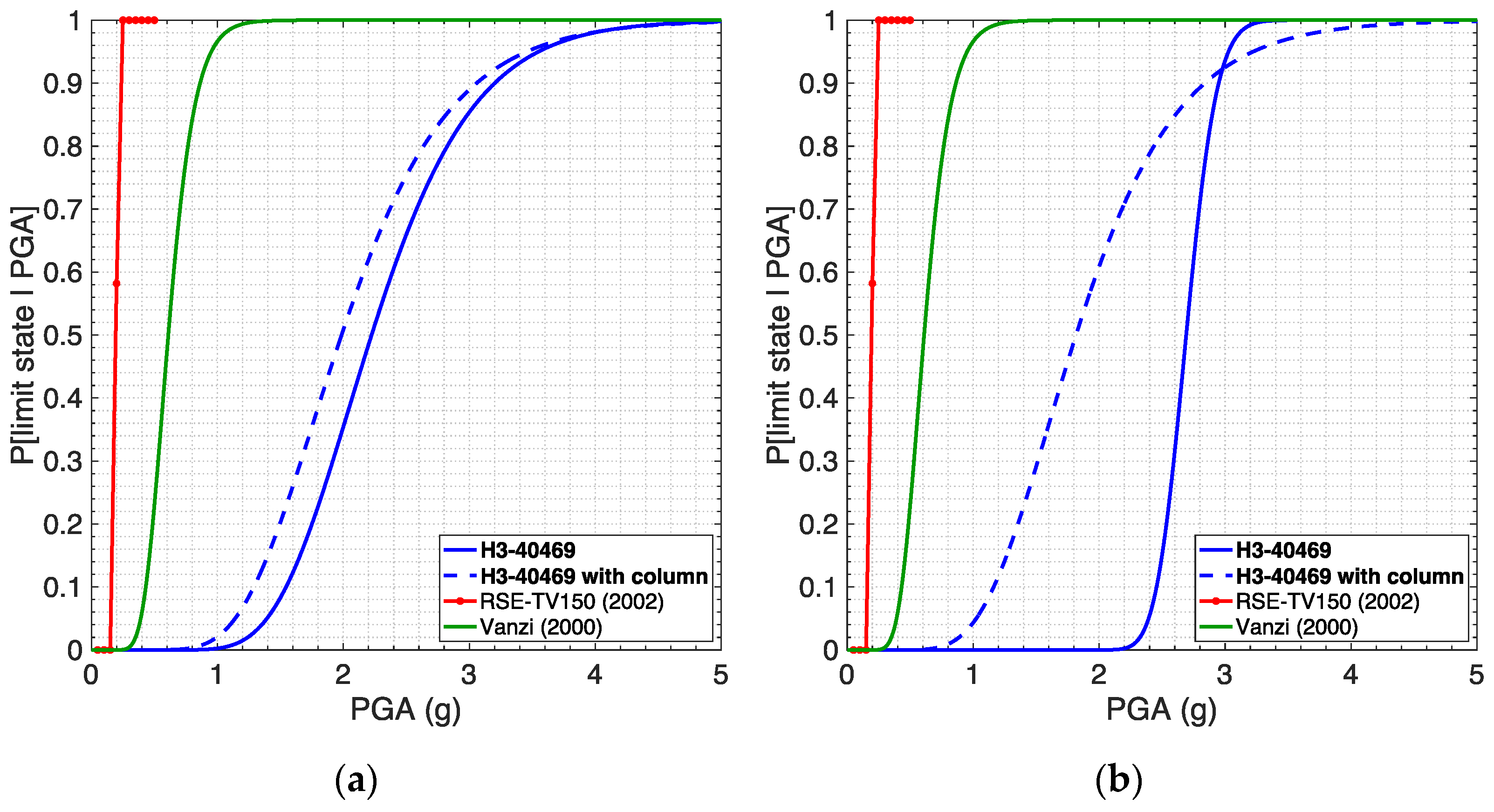
5.3. Comparison with Curves from the Literature

The last phase of this study was devoted to the comparison of the derived fragility curves, for the eight models and two soil types, with those available in the literature for voltage and current transformers. The latter were collected from three sources:
  • Database assembled by RSE (Gatti et al., 2002) [10], containing fragility curves for a number of electric devices, all mounted on different types of supporting structure. The curves selected for the comparison are those (i) related to voltage and current transformers operating in substations at 150 kV and 380 kV (voltage values similar to the ones of the devices investigated herein) mounted on a column, (ii) expressed as a function of PGA, and (iii) related to two different site conditions, namely rock and soil (with site amplification), to be compared with the curves obtained herein for soil types A and C, respectively.
  • Fragility curves selected and used within the European project SYNER-G (2012) [11], as reported in deliverable 3.3 (Pinto et al., 2010) [38] of SYNER-G and partially in Cavalieri et al. (2014) [39]. In particular, the curves selected for the comparison are those by Vanzi (2000) [12], without voltage distinction, and by HAZUS (FEMA, 2003) [13] for high voltage HV (115 kV) and extra-high voltage EHV (500 kV) for current transformers, whilst for voltage transformers the only available curves are those by Vanzi (2000) [12], also in this case without voltage distinction.
  • Fragility curves proposed by Baghmisheh and Estekanchi (2019) [4] for current transformers operating at extra-high voltage EHV (400 kV). The curves selected for the comparison are those related to unconnected devices, consistently with the methodology adopted herein, and two limit states, namely moderate and severe damage. These curves were also included in the plots related to the high voltage device (see Figure 14), for reference.
The following figures, Figure 14, Figure 15, Figure 16 and Figure 17, display the comparisons between the fragility curves derived in this study, in the versions with and without the column and for soil types A and C, and the selected ones from the literature. It can be readily observed that for the majority of devices (with the exception of H3-40469) the proposed curves are aligned with the ones from the literature, with observed differences being a natural consequence of the variations in experimental campaigns, modelling approaches, performance thresholds, and methodology employed to derive the fragility functions. In several cases, the proposed curves, derived through an approach that corresponds to the current state-of-the-art in the field of fragility models development, appear to be less conservative (i.e., with higher median PGA), especially for the H3-40469 with and without the column on both soil types, and the H3-34794 with the column on soil type A.

6. Conclusions

In this work, two voltage transformers and two current transformers designed for different system voltage levels (HV and EHV) were first tested on a shake table, and then numerically studied using finite element models calibrated against the experimental results. A number of nonlinear dynamic analyses were subsequently carried out within a multiple-stripe framework to derive a total of 16 fragility curves for the four transformers in their stand-alone and elevated/supported configurations, as well as two different soil types (rock and averagely dense soil). The three failure modes considered in the analyses, including mechanical failure of both steel and porcelain elements, as well as the disconnection of conductors at the top of the devices, allowed accounting for the limit states of collapse and loss of functionality. The obtained fragility curves encompass all the failure modes and limit states, thus producing a binary outcome (intact/broken) that can be used to predict if the device will remain operative or not given a seismic intensity level. Based on the derived curves, one of the voltage transformers, namely the H3-40469, is expected to experience light or negligible damage due to earthquake shaking, owing to its high resonance frequencies (and hence stiffness), whilst the remaining three devices may suffer moderate damage under medium to strong shaking intensities; however, their seismic risk is in effect mitigated by the presence of the typically employed supporting column. Finally, a comparison with other fragility curves currently available in the literature, limited in number especially for the case of voltage transformers, seems to indicate that the curves derived in this work can be used with confidence by analysts, infrastructure owners, emergency managers, and all the stakeholders engaged in mitigating the seismic risk of communities in earthquake-prone regions. In particular, having four fragility curves for each of the four instrument transformers investigated herein, the stakeholders can select the one that best fits their needs, in order to evaluate the damage state of these devices included in substations, within seismic risk assessment of electric power systems.

Author Contributions

Conceptualization, F.C. and R.P.; methodology, F.C., R.P., F.D., N.B. and M.d.N.; software, F.C. and G.D.; validation, F.C., G.D. and R.P.; formal analysis, F.C. and G.D.; investigation, F.C., G.D., R.P. and F.D.; resources, R.P. and F.D.; data curation, F.C. and F.D.; writing—original draft preparation, F.C. and G.D.; writing—review and editing, F.C., R.P., N.B. and M.d.N.; visualization, F.C. and G.D.; supervision, F.C., R.P., F.D., N.B. and M.d.N.; project administration, F.C., R.P. and F.D.; funding acquisition, R.P., N.B. and M.d.N. All authors have read and agreed to the published version of the manuscript.

Funding

This research was funded by the Research Fund for the Italian Electrical System under the contract agreement between RSE S.p.A. and the Ministry of Economic Development—General Directorate for the Electricity Market, Renewable Energy and Energy Efficiency, Nuclear Energy in compliance with the Decree of 16 April 2018.

Data Availability Statement

The data presented in this study are not publicly available.

Acknowledgments

The authors are particularly grateful to Trench Italia S.r.l. (Cairo Montenotte, SV, Italy) for kindly providing the four transformers tested in this work. The assistance of the laboratory technicians of the Eucentre Foundation, and the feedback and insight provided by staff at RSE S.p.A. are also acknowledged. In particular, special thanks go to Luigi Vadacca, whose support throughout the project was essential for its successful completion.

Conflicts of Interest

The authors declare no conflict of interest. The funders had no role in the design of the study; in the collection, analyses, or interpretation of data; in the writing of the manuscript; or in the decision to publish the results.

References

  1. Koliou, M.; Filiatrault, A.; Reinhorn, A.M.; Oliveto, N. Seismic Protection of Electrical Transformer Bushing Systems by Stiffening Techniques; Technical Report MCEER-12-0002; University at Buffalo: Buffalo, NY, USA, 2012. [Google Scholar]
  2. Zareei, S.A.; Hosseini, M.; Ghafory-Ashtiany, M. Seismic failure probability of a 400 kV power transformer using analytical fragility curves. Eng. Fail. Anal. 2016, 70, 273–289. [Google Scholar] [CrossRef]
  3. Zareei, S.A.; Hosseini, M.; Ghafory-Ashtiany, M. Evaluation of power substation equipment seismic vulnerability by multivariate fragility analysis: A case study on a 420 kV circuit breaker. Soil Dyn. Earthq. Eng. 2017, 92, 79–94. [Google Scholar] [CrossRef]
  4. Baghmisheh, A.G.; Estekanchi, H.E. Effects of rigid bus conductors on seismic fragility of electrical substation equipment. Soil Dyn. Earthq. Eng. 2019, 125, 105733. [Google Scholar] [CrossRef]
  5. Mohammadpour, S.; Hosseini, M. Experimental system identification of a 63 kV substation post insulator and the development of its fragility curves by dynamic finite element analyses. Earthq. Spectra 2017, 33, 1149–1172. [Google Scholar] [CrossRef]
  6. Gökçe, T.; Orakdöğen, E.; Yüksel, E. Failure mode investigation for High Voltage porcelain insulators. In Proceedings of the 16th European Conference on Earthquake Engineering, Thessaloniki, Greece, 18–21 June 2018. [Google Scholar]
  7. Gökçe, T.; Yüksel, E.; Orakdöğen, E. Seismic performance enhancement of high-voltage post insulators by a polyurethane spring isolation device. Bull. Earthq. Eng. 2019, 17, 1739–1762. [Google Scholar] [CrossRef]
  8. Gökçe, T.; Orakdöğen, E.; Yüksel, E. Improvement of the polyurethane spring isolation device for HV post insulators and its evaluation by fragility curves. Earthq. Spectra 2021, 37, 1677–1697. [Google Scholar] [CrossRef]
  9. Wen, B.; Moustafa, M.A.; Junwu, D. Seismic fragilities of high-voltage substation disconnect switches. Earthq. Spectra 2019, 35, 1559–1582. [Google Scholar] [CrossRef]
  10. Gatti, F.; Fratelli, M.; Bonacina, G. SISIGEN-SISTEL Impatto di Eventi Eccezionali sui Sistemi di Trasporto e Distribuzione dell’energia Elettrica. Contributo al Rapporto di Sintesi. Milestone 3; Technical Report Doc. RAT-ISMES-2238/2002; CESI S.p.A.: Milan, Italy, 2002. (In Italian) [Google Scholar]
  11. European Commission. SYNER-G. Collaborative Research Project, Funded by the European Union within Framework Programme 7 (2007–2013) under Grant Agreement No. 244061. 2012. Available online: http://www.vce.at/SYNER-G/files/project/proj-overview.html (accessed on 4 December 2022).
  12. Vanzi, I. Structural upgrading strategy for electric power networks under seismic action. Earthq. Eng. Struct. Dyn. 2000, 29, 1053–1073. [Google Scholar] [CrossRef]
  13. Federal Emergency Management Agency (FEMA). HAZUSMH MR4 Multi-Hazard Loss Estimation Methodology—Earthquake Model; Technical Manual; FEMA: Washington, DC, USA, 2003.
  14. Whittaker, A.S.; Fenves, G.L.; Gilani, A.S. Earthquake performance of porcelain transformer bushings. Earthq. Spectra 2004, 20, 205–223. [Google Scholar] [CrossRef]
  15. Koliou, M.; Filiatrault, A.; Reinhorn, A.M. Seismic response of high-voltage transformer-bushing systems incorporating flexural stiffeners II: Experimental study. Earthq. Spectra 2013, 29, 1353–1367. [Google Scholar] [CrossRef]
  16. Moustafa, M.A.; Mosalam, K.M. Substructured dynamic testing of substation disconnect switches. Earthq. Spectra 2016, 32, 567–589. [Google Scholar] [CrossRef]
  17. Oliveto, N.D.; Reinhorn, A.M. Evaluation of as-installed properties of transformer bushings. Eng. Struct. 2018, 162, 29–36. [Google Scholar] [CrossRef]
  18. McKenna, F.; Fenves, G.L.; Scott, M.H. OpenSees: Open System for Earthquake Engineering Simulation; Software; University of California: Berkeley, CA, USA, 2000; Available online: http://opensees.berkeley.edu (accessed on 4 December 2022).
  19. ICC-ES AC156; Seismic Certification by Shake-Table Testing of Nonstructural Components. ICC Evaluation Service: Brea, CA, USA, 2015. Available online: https://icc-es.org/acceptance-criteria/ac156/ (accessed on 4 December 2022).
  20. Eucentre. Curve di Fragilità di Trasformatori di Tensione e di Corrente; Technical Report RSE177E21_Rec-Report_EUC177-2021E; Eucentre Foundation: Pavia, Italy, 2021. (In Italian) [Google Scholar]
  21. Cavalieri, F.; Donelli, G.; Pinho, R.; Dacarro, F. Experimental response of voltage and current transformers tested on shake table. In Proceedings of the 17th European Conference on Earthquake Engineering, Bucharest, Romania, 4–9 September 2022. [Google Scholar]
  22. Yang, T.; Schellenberg, A. OpenSees Navigator; Software; University of California: Berkeley, CA, USA, 2004; Available online: https://openseesnavigator.berkeley.edu/downloads/ (accessed on 4 December 2022).
  23. MATLAB, Version R2019b. Software. The MathWorks Inc.: Natick, MA, USA, 2019. Available online: https://www.mathworks.com/products/matlab.html(accessed on 4 December 2022).
  24. OpenSeesWiki Website. Available online: https://opensees.berkeley.edu/wiki/index.php/Main_Page (accessed on 4 December 2022).
  25. Jalayer, F.; Cornell, C.A. Alternative non-linear demand estimation methods for probability-based seismic assessments. Earthq. Eng. Struct. Dyn. 2009, 38, 951–972. [Google Scholar] [CrossRef]
  26. Vamvatsikos, D.; Cornell, C.A. Incremental dynamic analysis. Earthq. Eng. Struct. Dyn. 2002, 31, 491–514. [Google Scholar] [CrossRef]
  27. Baker, J.W. Efficient analytical fragility function fitting using dynamic structural analysis. Earthq. Spectra 2015, 31, 579–599. [Google Scholar] [CrossRef]
  28. CEN EN 1998-1:2004; Eurocode 8: Design of Structures for Earthquake Resistance—Part 1: General Rules, Seismic Actions and Rules for Buildings. European Committee for Standardization: Brussels, Belgium, 2004.
  29. Bradley, B.A. A generalized conditional intensity measure approach and holistic ground-motion selection. Earthq. Eng. Struct. Dyn. 2010, 39, 1321–1342. [Google Scholar] [CrossRef] [Green Version]
  30. Bradley, B.A. A ground motion selection algorithm based on the generalized conditional intensity measure approach. Soil Dyn. Earthq. Eng. 2012, 40, 48–61. [Google Scholar] [CrossRef]
  31. Chiou, B.; Darragh, R.; Gregor, N.; Silva, W. NGA project strong-motion database. Earthq. Spectra 2008, 24, 23–44. [Google Scholar] [CrossRef] [Green Version]
  32. He, C.; Xie, Q.; Zhou, Y. Influence of flange on seismic performance of 1,100-kV ultra-high voltage transformer bushing. Earthq. Spectra 2019, 35, 447–469. [Google Scholar] [CrossRef]
  33. Rexton–Steel & Alloys Website. Available online: https://www.rextonsteel.com/s355j2-n-seamless-pipe-supplier-stockist.html#mechanical-properties (accessed on 4 December 2022).
  34. Henan Gang Iron and Steel Co., Ltd. Website. Available online: https://www.steel-biz.com/s690ql-steel-plates-manufacturer-supplier/#mechanical-properties (accessed on 4 December 2022).
  35. Gilani, A.S.; Chavez, J.W.; Fenves, G.L.; Whittaker, A.S. Seismic Evaluation of 196 kV Porcelain Transformer Bushings; Technical Report PEER-1998/02; University of California: Berkeley, CA, USA; Pacific Earthquake Engineering Research Center: Richmond, CA, USA, 1998. [Google Scholar]
  36. Anagnos, T. Development of an Electrical Substation Equipment Performance Database for Evaluation of Equipment Fragilities; Technical Report; Department of Civil and Environmental Engineering, San Jose State University: San Jose, CA, USA, 1999. [Google Scholar]
  37. Iervolino, I. Estimation uncertainty for some common seismic fragility curve fitting methods. Soil Dyn. Earthq. Eng. 2022, 152, 107068. [Google Scholar] [CrossRef]
  38. Pinto, P.E.; Cavalieri, F.; Franchin, P.; Vanzi, I. D3.3—Fragility Functions for Electric Power System Elements, Deliverable 3.3 of the SYNER-G Project; Sapienza University of Rome: Rome, Italy, 2010; Available online: http://www.vce.at/SYNER-G/files/dissemination/deliverables.html (accessed on 4 December 2022).
  39. Cavalieri, F.; Franchin, P.; Pinto, P.E. Fragility Functions of Electric Power Stations. In SYNER-G: Typology Definition and Fragility Functions for Physical Elements at Seismic Risk; Pitilakis, K., Crowley, H., Kaynia, A.M., Eds.; Springer: Dordrecht, The Netherlands; Heidelberg, Germany, 2014; pp. 157–185. ISBN 978-94-007-7872-6. [Google Scholar] [CrossRef]
Figure 1. Day 1 of the testing campaign: (a) UUT-1 and (b) UUT-2 mounted on the shake table.
Infrastructures 07 00171 g001
Figure 2. Day 2 of the testing campaign: (a) UUT-3 and (b) UUT-4 mounted on the shake table.
Infrastructures 07 00171 g002
Figure 3. Position and serial number of the accelerometers installed (a) on UUT-1 and UUT-2 and (b) on UUT-3 and UUT-4.
Infrastructures 07 00171 g003
Figure 4. Peaks (red dots) picked on FAS functions, for (a,b) UUT-1 X-,Y-dir., (c,d) UUT-2 X-,Y-dir., (e,f) UUT-3 X-,Y-dir., (g,h) UUT-4 X-,Y-dir., in the intact configuration (beginning of testing days).
Infrastructures 07 00171 g004
Figure 5. Adopted RRS for horizontal (X-dir. and Y-dir.) and vertical (Z-dir.) acceleration.
Infrastructures 07 00171 g005
Figure 6. 3D numerical models of the four transformers: (a) H3-40469, (b) H3-36523, (c) H3-35245, (d) H3-34794.
Infrastructures 07 00171 g006
Figure 7. Portion of the drawing related to transformer H3-40469 (numbers 1, 4 and 9 indicate the primary terminal, the porcelain insulator bushing and the lifting holes, respectively), with a photo and correspondent (indicated by a green arrow) numerical model of the spherical cap.
Infrastructures 07 00171 g007
Figure 8. 3D numerical models of the four transformers with the supporting column: (a) H3-40469, (b) H3-36523, (c) H3-35245, (d) H3-34794.
Infrastructures 07 00171 g008
Figure 9. Experimental–numerical comparisons of (left) acceleration and (right) displacement histories along the X-direction, at the initial lower intensity stage, for models (a,b) H3-40469, with close-up on three seconds of the trace, (c,d) H3-36523, (e,f) H3-35245, (g,h) H3-34794.
Infrastructures 07 00171 g009
Figure 10. Demands (in absolute value) of (a) maximum steel strain and (b) maximum top displacement, obtained via MSA for model H3-35245 without the supporting column and for soil type A.
Infrastructures 07 00171 g010
Figure 11. Fragility curve, with indication of the lumped fragility points, obtained via ML for model H3-35245 without the supporting column and soil type A.
Infrastructures 07 00171 g011
Figure 12. Ensemble of the 16 fragility curves obtained, grouped for models (a) without the column and (b) with the column.
Infrastructures 07 00171 g012
Figure 13. Ensemble of the 16 fragility curves obtained, grouped for (a) soil type A (b) soil type C.
Infrastructures 07 00171 g013
Figure 14. Comparison between the obtained curves and the ones from the literature for current transformers employed in HV substations, for (a) soil type A and (b) soil type C. Cited references are: Gatti et al. (2002) [10], Vanzi (2000) [12], FEMA (2003), Baghmisheh and Estekanchi (2019) [4].
Infrastructures 07 00171 g014
Figure 15. Comparison between the obtained curves and the ones from the literature for current transformers employed in EHV substations, for (a) soil type A and (b) soil type C. Cited references are: Gatti et al. (2002) [10], Vanzi (2000) [12], FEMA (2003), Baghmisheh and Estekanchi (2019) [4].
Infrastructures 07 00171 g015
Figure 16. Comparison between the obtained curves and the ones from the literature for voltage transformers employed in HV substations, for (a) soil type A and (b) soil type C. Cited references are: Gatti et al. (2002) [10], Vanzi (2000) [12].
Infrastructures 07 00171 g016
Figure 17. Comparison between the obtained curves and the ones from the literature for voltage transformers employed in EHV substations, for (a) soil type A and (b) soil type C. Cited references are: Gatti et al. (2002) [10], Vanzi (2000) [12].
Infrastructures 07 00171 g017
Table 1. Main technical specifications for the four specimens.
SpecimenUUT1UUT2UUT3UUT4
Type and voltage (kV)VT 170VT 420CT 170CT 420
ApparatusVEOT 170TCVT 420IOSK 170IOSK 420
Production nameH3-40469H3-36523H3-35245H3-34794
Plan dimensions (m)0.698 × 0.7190.508 × 0.6380.890 × 0.9800.674 × 0.880
Total height (m)2.443.872.974.68
Total mass (kg)400533540900
Constitutive materialsPorcelain, steel,
aluminium
GFRP 1, silicone rubber HTV 2,
steel, aluminium
1 Glass Fiber Reinforced Polymer, also called fiberglass; 2 High temperature vulcanized.
Table 2. First two resonance frequencies (X- and Y-directions) identified for the specimens in the intact configuration (beginning of testing days).
SpecimenUUT1UUT2UUT3UUT4
Frequency in X-dir. (Hz)19.44.12.22.1
Frequency in Y-dir. (Hz)17.54.12.22.1
Table 3. First two resonance frequencies (X- and Y-directions) identified for the specimens in the possibly damaged configuration (end of testing days).
SpecimenUUT1UUT2UUT3UUT4
Frequency in X-dir. (Hz)18.94.02.22.1
Frequency in Y-dir. (Hz)17.24.12.22.0
Table 4. Comparison of the first two experimental and numerical eigenfrequencies (X- and Y-directions) of the models.
ModelH3-40469H3-36523H3-35245H3-34794
Experimental
eigenfrequencies (Hz)
19.40–17.504.10–4.102.20–2.202.10–2.10
Numerical
eigenfrequencies (Hz)
19.21–17.304.17–4.182.22–2.222.11–2.11
Table 5. First two eigenfrequencies (X- and Y-directions) of the models equipped with the supporting column.
ModelH3-40469H3-36523H3-35245H3-34794
Numerical
eigenfrequencies (Hz)
5.35–4.733.49–3.721.88–1.831.86–1.98
Table 6. Failure modes, limit states and EDPs adopted.
Failure ModeLimit StateEDP
Mechanical failure of steel
in the base elements
Moderate damage or
collapse
Maximum strain in the base steel elements
Disconnection of conductors at the topLoss of functionalityMaximum top displacement
Mechanical failure of
porcelain in the sheds and base elements
CollapseMaximum strain in the porcelain sheds and base elements
Table 7. Parameter values for the 16 fragility curves obtained in this study.
TransformerSoil Type ASoil Type C
Median PGA (g)DispersionMedian PGA (g)Dispersion
H3-404692.2240.2842.6910.071
H3-365230.3980.4490.3910.429
H3-352450.4880.5310.3940.576
H3-347940.3550.6400.2830.610
H3-40469 with column1.9860.3371.8170.348
H3-36523 with column0.4030.4110.3770.373
H3-35245 with column0.5510.6690.4570.620
H3-34794 with column1.3031.0100.6780.491
Publisher’s Note: MDPI stays neutral with regard to jurisdictional claims in published maps and institutional affiliations.

