Automatic Detection of Dynamic and Static Activities of the Older Adults Using a Wearable Sensor and Support Vector Machines


1
Machine Learning Algorithms Team, Glassdoor, Mill Valley, CA 94941, USA
2
Department of Physical Therapy, Crean College of Health and Behavioral Sciences, Chapman University, Orange, CA 92866, USA
3
Department of Electrical Engineering and Computer Sciences, Fowler School of Engineering, Chapman University, Orange, CA 92866, USA
4
School of Biological and Health Systems Engineering, Arizona State University, Tempe, AZ 85281, USA
*
Author to whom correspondence should be addressed.
Sci 2020, 2(3), 62; https://0-doi-org.brum.beds.ac.uk/10.3390/sci2030062
Submission received: 30 March 2020
/
Accepted: 8 May 2020
/
Published: 3 August 2020
Abstract
:Although Support Vector Machines (SVM) are widely used for classifying human motion patterns, their application in the automatic recognition of dynamic and static activities of daily life in the healthy older adults is limited. Using a body mounted wireless inertial measurement unit (IMU), this paper explores the use of SVM approach for classifying dynamic (walking) and static (sitting, standing and lying) activities of the older adults. Specifically, data formatting and feature extraction methods associated with IMU signals are discussed. To evaluate the performance of the SVM algorithm, the effects of two parameters involved in SVM algorithm—the soft margin constant C and the kernel function parameter —are investigated. The changes associated with adding white-noise and pink-noise on these two parameters along with adding different sources of movement variations (i.e., localized muscle fatigue and mixed activities) are further discussed. The results indicate that the SVM algorithm is capable of keeping high overall accuracy by adjusting the two parameters for dynamic as well as static activities, and may be applied as a tool for automatically identifying dynamic and static activities of daily life in the older adults.
1. Introduction
Fall accidents are a significant problem for the older adults [1,2,3], and several studies have shown that fall risks in this population can be identified with motion patterns associated with the activities of daily life [4,5]. While the classification of dynamic and static activities of daily life is a key point for fall prevention research efforts, the greater variability of motion patterns associated with aging [6,7,8,9,10] and its effect on classification performance are not well understood. In this study, we investigate the use of support vector machine (SVM) classifier to identify dynamic as well as static activities of daily life in the older adults.
Numerous classification algorithms exist to provide human motion classification patterns, such as the wavelet method, the linear discriminant analysis (LDA) method, the ambient assisted living (AAL) systems, the Multi-Classifier Adaptive-Training (MCAT) algorithm, the pervasive neural network algorithm, ambient intelligence, and the SVM algorithm. Specifically, gyroscope data and the wavelet method was used to analyze the “sit-to-stand” transition in relation to fall risk by Najafi et al. [11]. A linear discriminant analysis method was adopted to classify external load conditions during walking by Lee et al. [12]. An Evaluating Assisted Ambient Living (EvAAL) workshop aimed to address the problem of localization and tracking issues for AAL, and provided a novel approach to evaluate and assess AAL systems and services [13]. A Multi-Classifier Adaptive-Training algorithm (MCAT) was proposed to improve the classifier for activity recognition by Cvetković et al. [14]. A pervasive neural network algorithm was utilized by Kerdegari et al. on smart phones to monitor older individuals’ activities, and identified the occurrence of falls [15]. Ambient intelligence was used to gather information from an environment to assess patients’ vital signs and locations in the waiting area of a hospital emergency department by Curtis et al. [16]. In addition, the SVM classifier was used to analyze the minimum foot clearance owing to aging by Begg et al. [17]. The SVM is considered a powerful technique for general data classification, and has been widely used to classify human motion patterns with good results [18,19,20,21]. The advantage of the SVM algorithm is that it can generate a classification result with limited data sets by minimizing both structural and empirical risks [22].
Although numerous studies have been devoted to improving the SVM algorithms, little work has been performed on assessing the robustness of SVM algorithms associated with movement variations (i.e., mixed activities of daily life) of the older adults [23]. In this study, we investigate variations of the optimal parameters involved in the SVM algorithm by taking a closer look into the performance of SVM classifier for detecting dynamic and static motions of the older adults. Furthermore, step-by-step procedures associated with the SVM classification are elaborated to provide a better understanding of the classification method utilizing an ambulatory inertial measurement unit system for biomedical applications.
2. Methods and Materials
2.1. SVM
Here, some basic concepts applied in SVMs are elaborated in light of the classification schemes. The SVM is a statistical method introduced by Guyon and Vapnik [24,25] which has been widely applied to different classification needs [26,27,28]. The idea of the SVM algorithm is to map the original data to a high-dimensional space using nonlinear mapping by finding an optimum linear separating hyperplane with the maximal margin in this higher dimensional space [24,25].
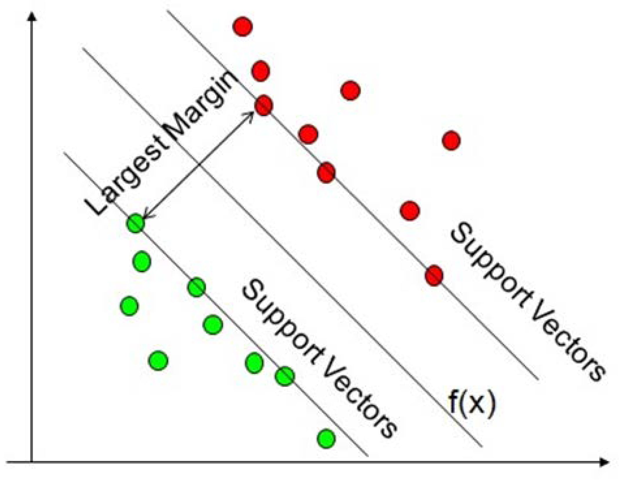
The SVM is a principled approach to machine learning utilizing concepts from classical statistical learning theory [24,29,30]; it exhibits good generalization of new data with a readily interpretable model. Additionally, learning involves the optimization of a convex function (i.e., one solution). From the perspective of statistical learning theory, the motivation for considering binary classifier SVM comes from the theoretical bounds on the generalization error. These generalization bounds have two important features: the upper bound is independent of the size of the input space, and the bound is minimized by maximizing the margin between the hyperplane separating the two classes and the closest data point to each class—called support vectors. Closest points are called support vectors because they support where the hyperplane should be located, that is, moving the nonsupport vectors will not shift the hyperplane, whereas moving the support vectors will shift the hyperplane (Figure 1).
The basis of the SVM algorithm can be stated as follows: training data set is given, containing data feature vectors and the corresponding data labels , in the form of
where , m is dimension of the feature (real) vector, , and n is the number of samples. In our case, as for dynamic activities and is employed for static activities. We assume is some unknown function to classify the feature vector .
In the SVM method, optimal margin classification for linearly separable patterns is achieved by finding a hyperplane in m dimensional space. The linear classifier is based on a linear discriminant function of the form
where the vector is the weight vector and b is the hyperplane bias. We try to find the maximum margin hyperplane dividing the points having from those having . In our case, two classes from the samples are labeled by for dynamic motion class ( and for static motion class (, while is called the hyperplane which separates the sampled data linearly.
In many cases, a linear classifier cannot satisfy the demand of accuracy due to its simplicity; thus, a more sensitive classifier is needed for real-world applications. Correspondingly, kernel theory was introduced by implicitly mapping data from the input space into higher dimensional space, in order to achieve nonlinear transformation and avoid the problem of dimensionality [31]. The kernel function can be expressed as and is related to by
where represents the nonlinear feature mapping function, ,
The evaluation of a hyperplane in feature space is usually determined by the distance between the hyperplane and the training points lying closest to it, which are named support vectors (Figure 1). Therefore, it is necessary to search for an optimal separating hyperplane to maximize the distance between the support vectors and the hyperplane [31]. The distance from the hyperplane to a support vector is ; thus, we can get the distance between the support vectors of one class to the other class simply by using geometry: .
As real-life datasets may contain noise, and SVM can fit this noise leading to poor generalization, the effects of outliers and noise can be reduced by introducing a soft margin. The soft-margin minimization problem relaxes the strict discriminant by introducing slack variables, , and is formulated as
The Lagrange theory is applied to solve Equation (5), and we can get the solved dual Lagrangian form of minimize
where are the non-negative Lagrangian multipliers, and C is a constant parameter, called the regularization parameter, which determines the tradeoff between the maximum margin and minimum classification error.
Once we have found the Lagrangian multipliers , then the optimal can be obtained:
Correspondingly, the value of optimal can be derived from the constraints
Thus, we can obtain the optimal value:
At this point, we have all of the necessary parameters to write down the decision function needed to predict the classification of a new data point :
In essence, finding and and applying the choice of kernel to the decision function will classify new data points as either dynamic or static activities. In general, if is nonzero, it is a support vector, while if is zero, it is not a support vector. Intuitively, as illustrated in Figure 1, moving the nonsupport vector will result in no shift of the hyperplane (i.e., is zero).
The process of obtaining the quadratic program solution is known as training, and the process of using the trained SVM model to classify new data sets is known as testing. In this paper, two types of human activities are separately presented as input for the training of the SVM model, labeled with the dynamic and static types [ for dynamic, for static]. Data processing of the raw data and feature extraction methods are discussed next within the empirical paradigm.
The motion patterns associated with activities of daily life (walking, standing, sitting and lying) were captured by the wearable inertial measurement unit (IMU—accelerometer and gyroscope) system. Afterwards, we employed the SVM method to classify dynamic and static activities. The selection of features and formatting of the data into the SVM input file is further elaborated in light of analyzing human movements utilizing IMU signals. Subsequently, we investigated the effects of two parameters pertinent to SVM classifiers: soft margin constant C and the kernel function parameter . The motion associated with dynamic (normal walking is assumed here to be dynamic) and static activities (e.g., lying, sitting, standing still with eyes open and closed) of the older adults were investigated.
2.2. Participants and Data Collection
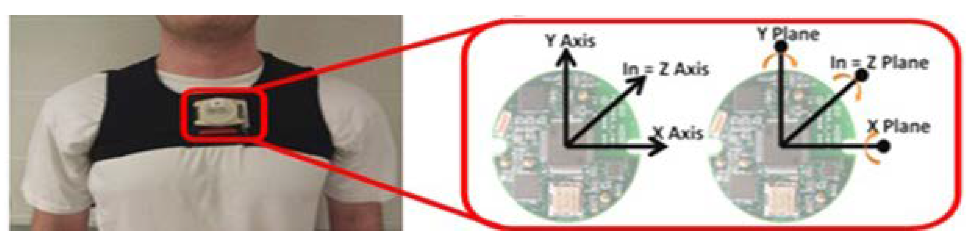
Thirty community dwelling healthy older individuals consisting of 21 females and 9 males (Height 1.68 ± 0.09 m, Weight 162.09 ± 22.33 lb, Age 76 ± 7 years) from Loudoun County, Virginia participated in this study. The data was collected from the local senior center. Written consent was provided by the participants who agreed to volunteer in the study. Participants wore three Inertial Measurement Unit (IMU) nodes [32]: one at the sternum level and another two on the lateral sides of the shank. In this manuscript, only the data from the sternum level node is analyzed (Figure 2). Participants were instructed to sit comfortably using a backrest for one minute on a 40 cm popliteal height chair. They were then instructed to stand up using the arm-rests. Postural sway data was collected while standing still with eyes open and eyes closed for 90 s. Next, the participants were instructed to lie down on their back (i.e., in supine posture) on a massage bench for a minute, and data were recorded for lying down. Afterwards, participants were asked to walk a distance of 10 m. Participants willingly volunteered for this experiment, and no compensation was provided. All participants signed an informed consent form approved by the Institutional Review Board at Virginia Tech (IRB Number 11-1088 [33]).
2.3. Instrumentation
The IMU node consisted of MMA7261QT tri-axial accelerometers (NXP Semiconductor, Netherlands) and IDG-300 (x and y plane gyroscope) (InvenSense, Santa Clara, CA, USA) and an ADXRS300 (Analog Devices, Norwood, MA, USA) z-plane uniaxial gyroscope aggregated in the TEMPO [32] platform (Technology-Enabled Medical Precision Observation which was manufactured in collaboration with the research team of the University of Virginia). Data acquisition was carried out using a Bluetooth adapter and laptop through a custom-built LabView VI(National Instruments, Austin, TX, USA). Data were acquired with a sampling frequency of 128 Hz. This frequency is largely sufficient for human movement analysis in daily activities which occur at low bandwidth [0.8–5 Hz] [34]. The data was processed using custom software written in MATLAB (MathWorks, Natick, MA, USA) and libSVM toolbox [35].
2.4. Data Analysis
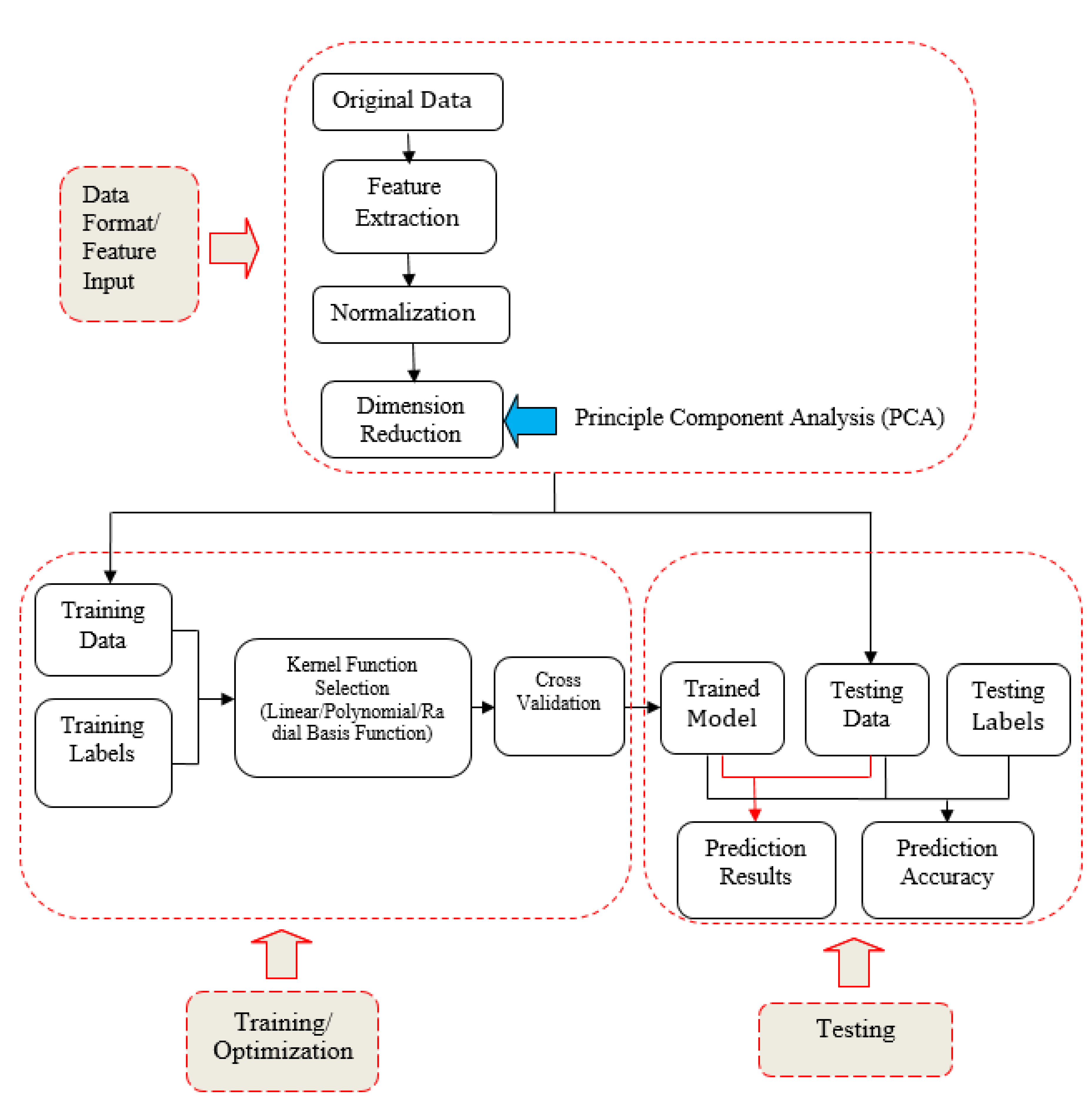
Thirty sets of data were used for training, and thirty sets of data were used for testing. Both training data and testing data contained ten dynamic activities and twenty static activities. First, the original IMU data were scaled to conveniently solve large datasets; then, Principle Component Analysis (PCA) [36,37] was employed to decrease the dimensions. Subsequently, the SVM algorithm was utilized to classify the human motion patterns (Figure 3).
- Step 1 Input of the Original Data
The original data is represented by an IMU at the sternum. The IMU provided three directional accelerations and angular velocities. The format of the original data is 9920 × 6 matrix with the row representing the time and the column representing 6 channel signals from tri-axial accelerometers and gyroscopes.
A total of 60 datasets (30 participants and 2 trials) containing 20 dynamic physical activities (walking) and 40 static activities were selected for movement classification. Each activity was represented by one two-second data segment. All of the datasets were split into training datasets and test datasets equally. In the first comparison (walking vs. lying), 20 normal walking segments were chosen as the dynamic activity, and 40 lying segments were chosen as the static activity. The datasets were then divided into training and testing sets, each containing 10 dynamic activities and 20 static activities. In the second comparison (walking vs. standing with eyes closed), 20 normal walking segments were chosen as the dynamic activity, and 40 standing still with eyes closed segments were chosen as the static activity. In the third comparison (walking vs. lying, sitting, standing still with eyes open and closed), 20 normal walking segments were chosen as the dynamic activity, and four different activities, i.e., lying, sitting, standing still with eyes open and closed, were selected as the static activity; each of them was assigned 10 segments, and thus, in total, there were 40 static activities.
- Step 2 Feature Extraction
Generally speaking, the features can be extracted from the time domain, frequency domain, and other data processing techniques, such as wavelet [38] and empirical mode decomposition [39,40]. Based on the criterion of minimizing computational complexity and maximizing the class discrimination, several key features are proposed for SVM classification [41].
- (1)
- Mean Absolute Value—the mean absolute value of the original signal, , in order to estimate signal information in time domain:where is the kth sampled point and N represents the total sampled number over the entire signal.
- (2)
- Zero Crossings—the number of times the waveform crosses zero, in order to reflect signal information in the frequency domain.
- (3)
- Slope Sign Changes—the number of times the slope of the waveform changes sign, in order to measure the frequency content of signal.
- (4)
- Waveform Length—the cumulative curve length over the entire signal, in order to provide information on the waveform complexity.
All of these feature values will give a measure of waveform amplitude, frequency, and duration within a single parameter. And they were extracted from raw signals to create the total feature sets for representing the dynamic or static motion patterns. After feature extraction, the original data were transformed to the feature data with a 60 × 24 matrix. The row number 60 means 60 total data sets to test as described above, and the column number of 24 is obtained from 4 features in each of the 6 channels. Thirty data sets were selected for the training data; thus, the size of the training data was 30 × 24.
- Step 3 Normalization
The above data were then normalized by each column to a range between 0 and 1.
- Step 4 Principle Component Analysis (PCA)
The objective of PCA is to perform dimensionality reduction while preserving as much of the randomness in the high-dimensional space as possible. The PCA algorithm can be described as:
- (1)
- Assume X is an m × n matrix, and choose a normalized direction in m-dimensional space along which the variance in X is maximized, saving this vector as .
- (2)
- Find another direction along which variance is maximized; however, the search is restricted to all directions orthogonal to all previous selected directions due to the orthonormality condition, saving this vector as . The procedure is repeated until m vectors are selected. The resulting ordered set of p is called principal components.
The dimension reduction can be described as:
- (1)
- For the m eigenvectors, we reduce from m dimensions to k dimensions by choosing k eigenvectors related to k largest eigenvalues ;
- (2)
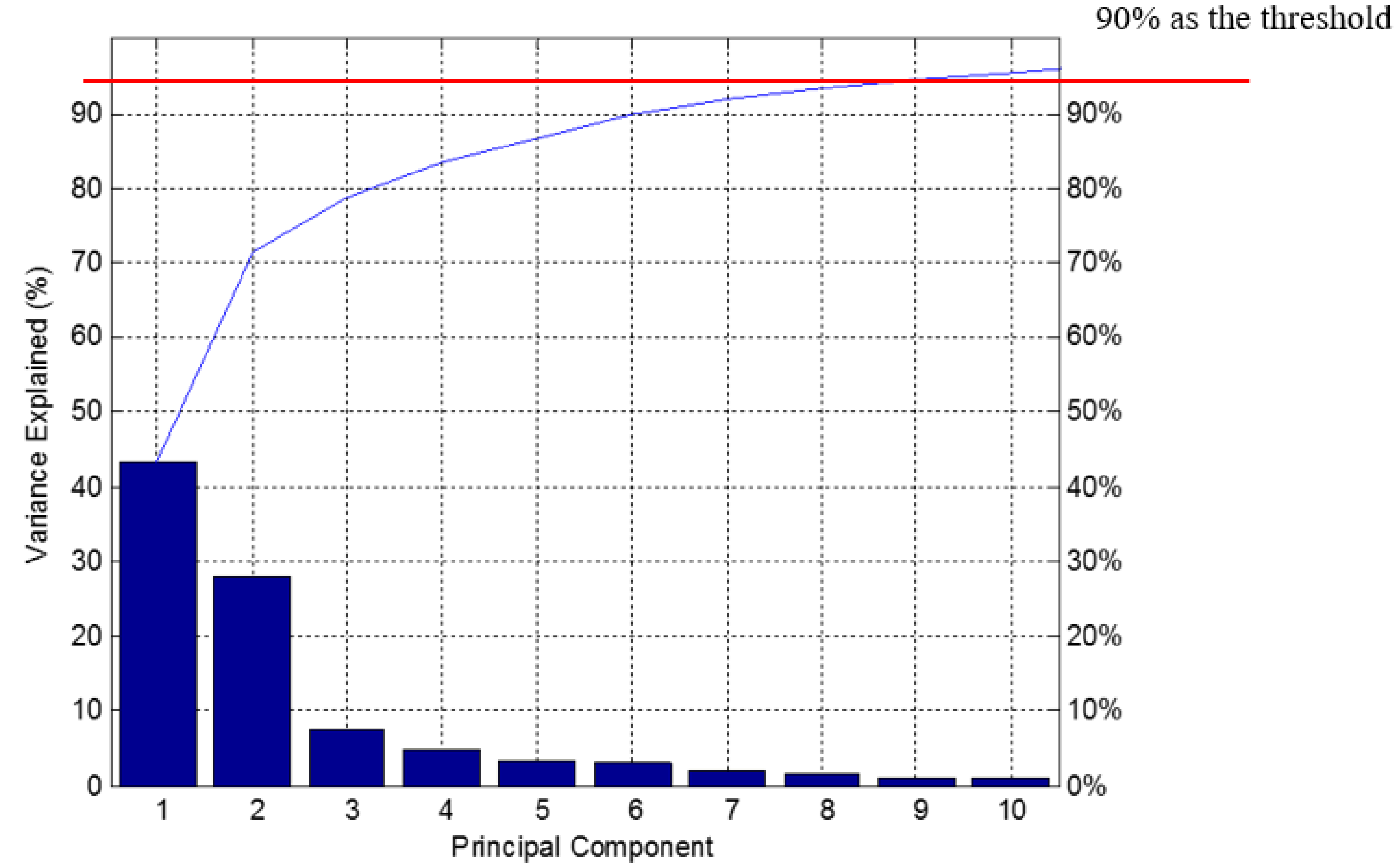
- Proportion of Variance (PoV) can be explained as:where are sorted in descending order, and the threshold of PoV is typically set as 0.9.
In our case, the m value should be 24. From the figure below (Figure 4), it can be found that when k reaches 7, the PoV will be above 0.9. Therefore, the PCA approach reduces the dimension of the original data from 24 to 7. Figure 4 illustrates the principal components based on the variance values. Additionally, Figure 5 illustrates three principal components from the model, and it can be readily seen that although “standing” and “walking” can be distinguished easily, other activities may not. After the dimension reduction by PCA, the dataset is reduced as a matrix of 30 × 7.
- Step 5 SVM Classifier Testing
Three criteria were used to assess the performance of the SVM classifier.
where TP represents the number of true positive; here, it refers to dynamic activities. TN is the number of true negatives, and it labels as static activities. FP is the number of false dynamic activity identification, and FN is the number of false static activity identification. While accuracy indicates the overall detection accuracy for all the activities, sensitivity is defined as the ability of the SVM classifier to accurately recognize the dynamic activities. Specificity indicates the SVM classifier’s ability to avoid false detection.
Furthermore, a receiver operating characteristic (ROC) curve was also used to evaluate the SVM classifier’s performance. ROC analysis is generally utilized to select optimal models and to qualify the accuracy of diagnostic tests. The area under the ROC curve (AUC) which is a representation of the classification performance was utilized to assess the effectiveness of the SVM classifier.
3. Results
In this section, we first introduce the effects of the Gaussian kernel function on minimizing the upper bound on the expected test error. Afterwards, a selection of the optimal hyperparameters is discussed. The results from the three classification tests are discussed in light of the three criteria discussed earlier (accuracy, sensitivity, selectivity).
3.1. Effect of SVM Key Parameters on Classification
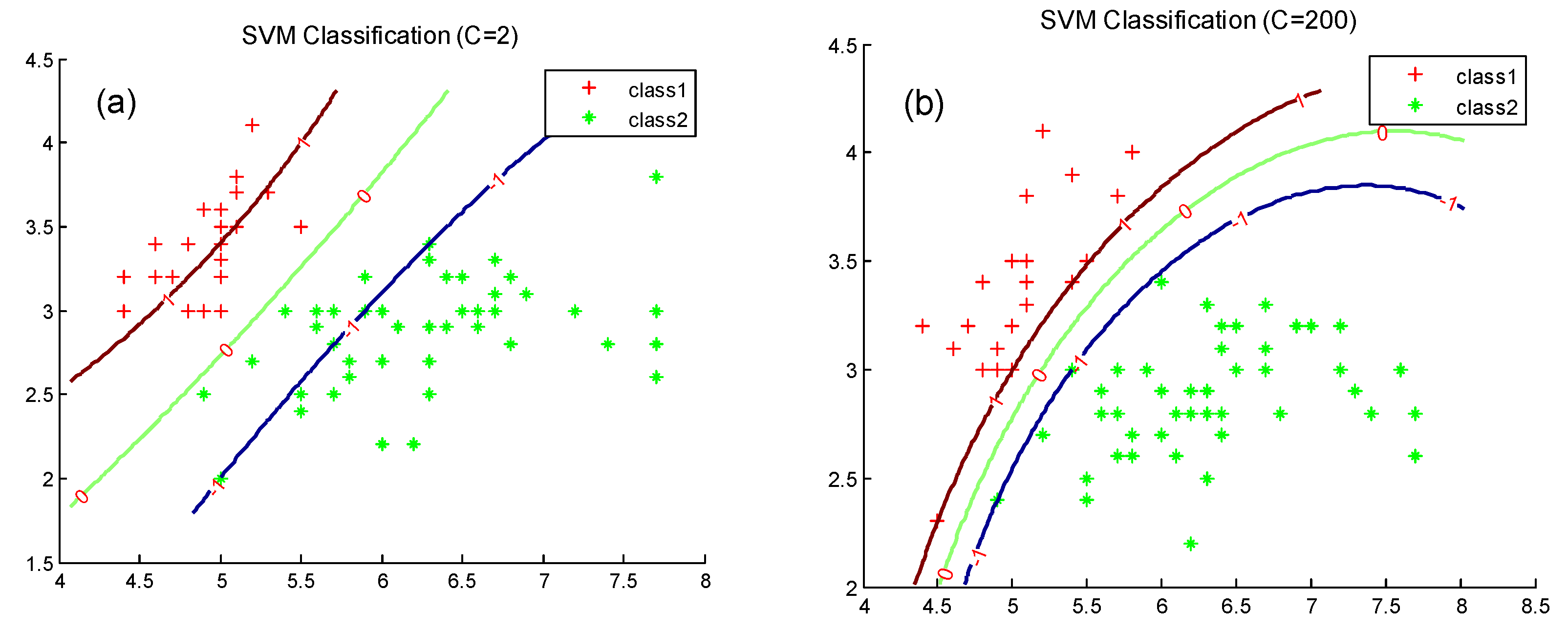
The SVM algorithm has two important parameters called hyperparameters: soft margin constant C, and the other parameter reflecting the kernel function. In this paper, a Gaussian kernel was applied to the SVM classifier; correspondingly, the other parameter, , refers to the width of the Gaussian kernel. Parameter C reflects the tradeoff between the margin of error. When C is large, the margin of error is small; however, the margin becomes narrow as a penalty. When C is small, those points close to the boundary become the margin of error, but the hyperplane’s orientation will change, providing a much larger margin for the rest of the data.
As for , let’s first take a look at the Gaussian kernel:
The Gaussian basis function with center and variance can be constructed as
where is the dimensional number of Gaussian RBF.
If we construct SVM Gaussian RBF classifier as
where ; is known as the weight vector, is a bias term, is Lagrangian multipliers and c is the constant. To optimally choose the centers of , the center points which are critical to the classification task are selected. In other words, if unknown sample x goes away from the known sample centers of , there will be a decay, and we can use this kernel to assign weights (i.e., decision weights). The Support Vector Machine (SVM) algorithm implements this idea. The algorithm automatically computes the number and location of the above centers, and provides weights and the bias b in virtue of the Gaussian kernel function. Therefore, in the RBF kernel case, the SVM classifier utilizes the Gaussian kernel function to select centers, weights and apply a threshold in order to minimize an upper bound on the expected test error. The advantage of the RBF approach is that it utilizes local approximators to map input to output, so that the system computes rapidly and requires fewer training samples.
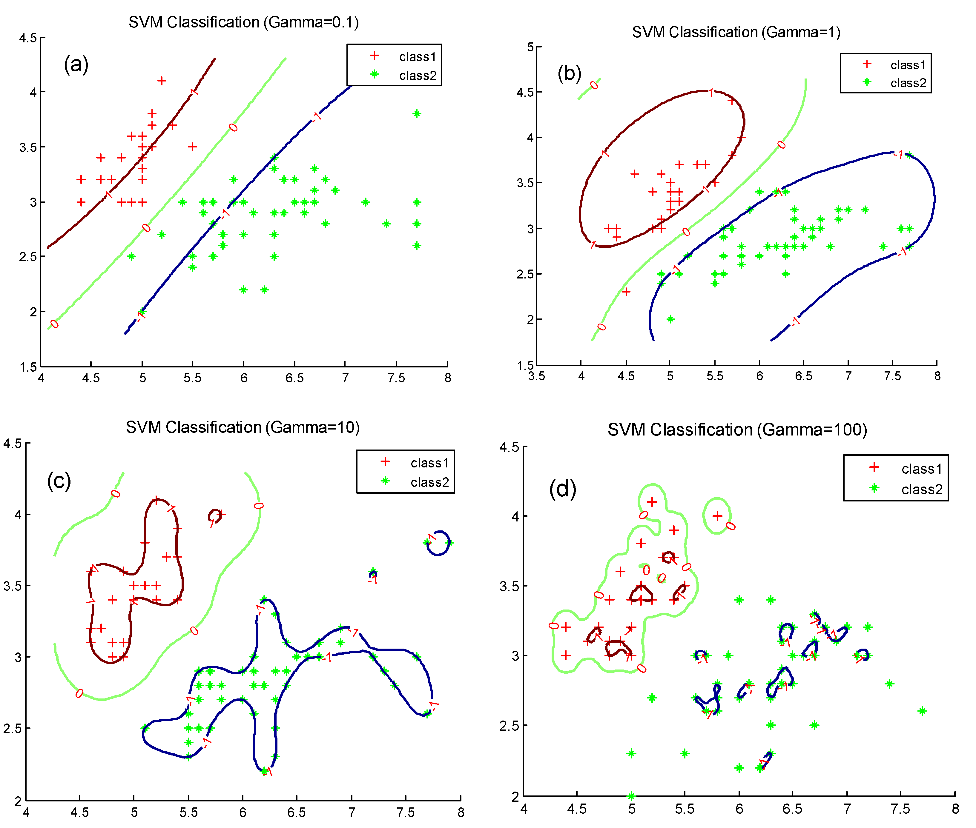
In essence, reflects the flexibility of the decision boundary. When is small, it generates a smooth decision boundary, i.e., one that is nearly linear. When is large, it generates a great curvature of the decision boundary. When is too large, it will cause overfitting, as shown in Figure 6d. Figure 6 and Figure 7 illustrate the effect of these two parameters, and C, on the decision boundary.
3.2. Optimization on SVM Key Parameters
To find the optimal values for the two parameters, cross-validation and a grid-search were utilized. In v-fold cross-validation, v means the number of input data splits. The training data is divided into v subsets equally. Any v-1 subset is selected for training the model, and then the remaining subset is predicted based on the constructed model. The same procedure is rotated in all the subsets while keeping the equal chance being predicted for each subset. Therefore, each subset of the input data will be predicted once, so the cross-validation accuracy is the percentage of data which is correctly classified.
An approach combining the grid-search method and cross-validation was proposed for searching for the optimal C and . Different pairs of (C, ) values were used for predicting data, and only the best cross-validation accuracy was selected. There were only two parameters for the search, and thus, it did not require too much computational time, satisfying the demand of SVM classification.
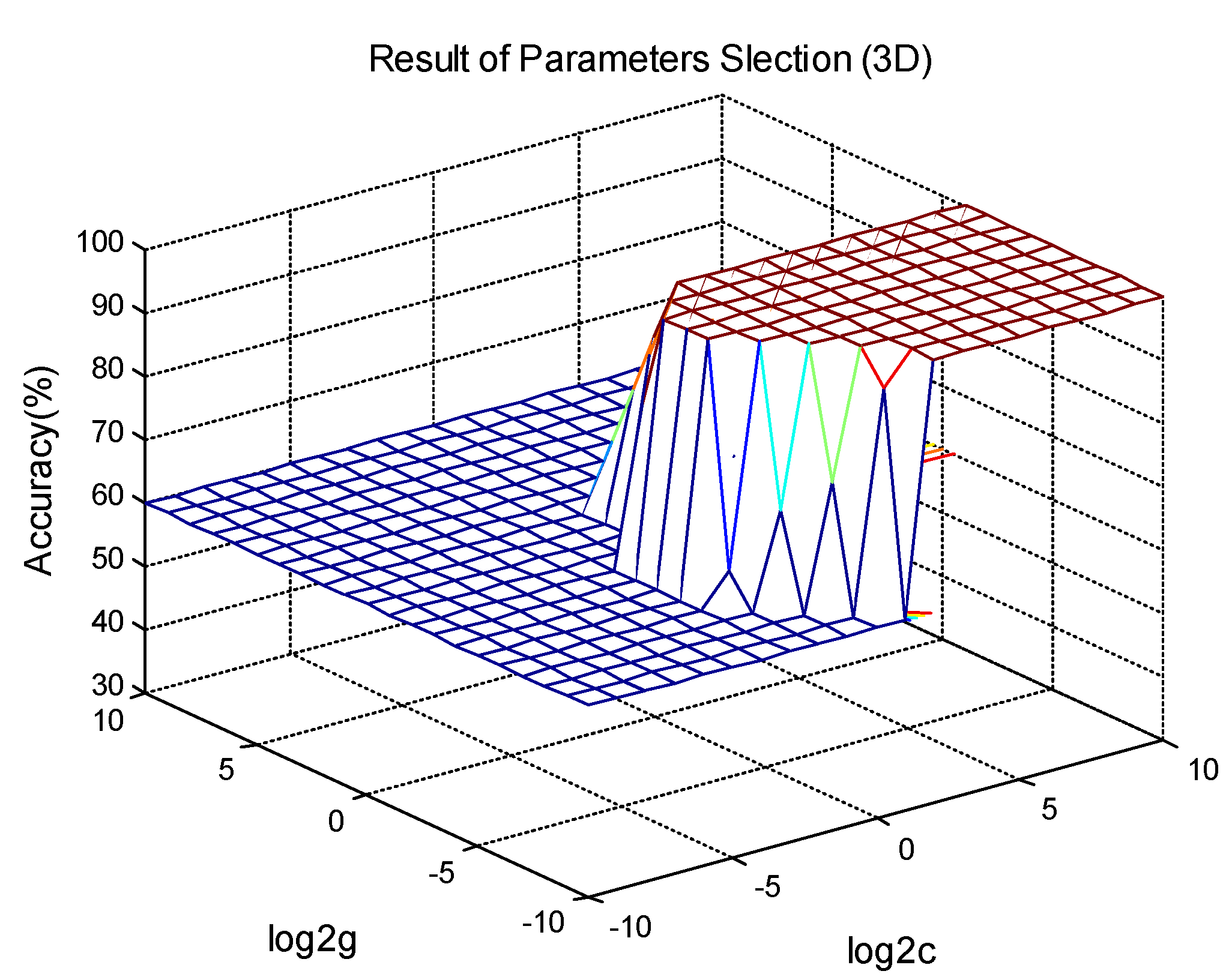
Here is a case of the SVM classification result comparison between the random parameters and optimal parameters. Firstly, 60 sets of data were split into training data and test data evenly, and then LibSVM with random SVM parameters was used to obtain a classification accuracy of 60%. Next, the grid-search and cross validation methods were applied to find the optimal C and values (the effects of selecting the optimal C and value, as compared to selecting the parameters at random, are illustrated in Figure 8).
It can be easily seen that the validation accuracy increases from 60% to 100%; however, there were several solution-sets of C and achieving the 100% accuracy. Here, the minimum C value was chosen as the optimal C, and the corresponding was chosen as the optimal value, since a high C value can improve the validation accuracy; however, it would also cause over-learning, and would affect the final classification prediction accuracy. Therefore, the optimal C was chosen as 0.2500 and was chosen as 0.0313 in this case.
3.3. Robustness of SVM Algorithm
As the assessment of human motion characteristics are linked to understanding the unwanted (i.e., noises) as well as wanted signals, it is important to understand the capability of the SVM classifier to effectively address noisy data. Therefore, the change of the parameters involved in the SVM algorithm, along with the added white and pink noise, was be investigated.
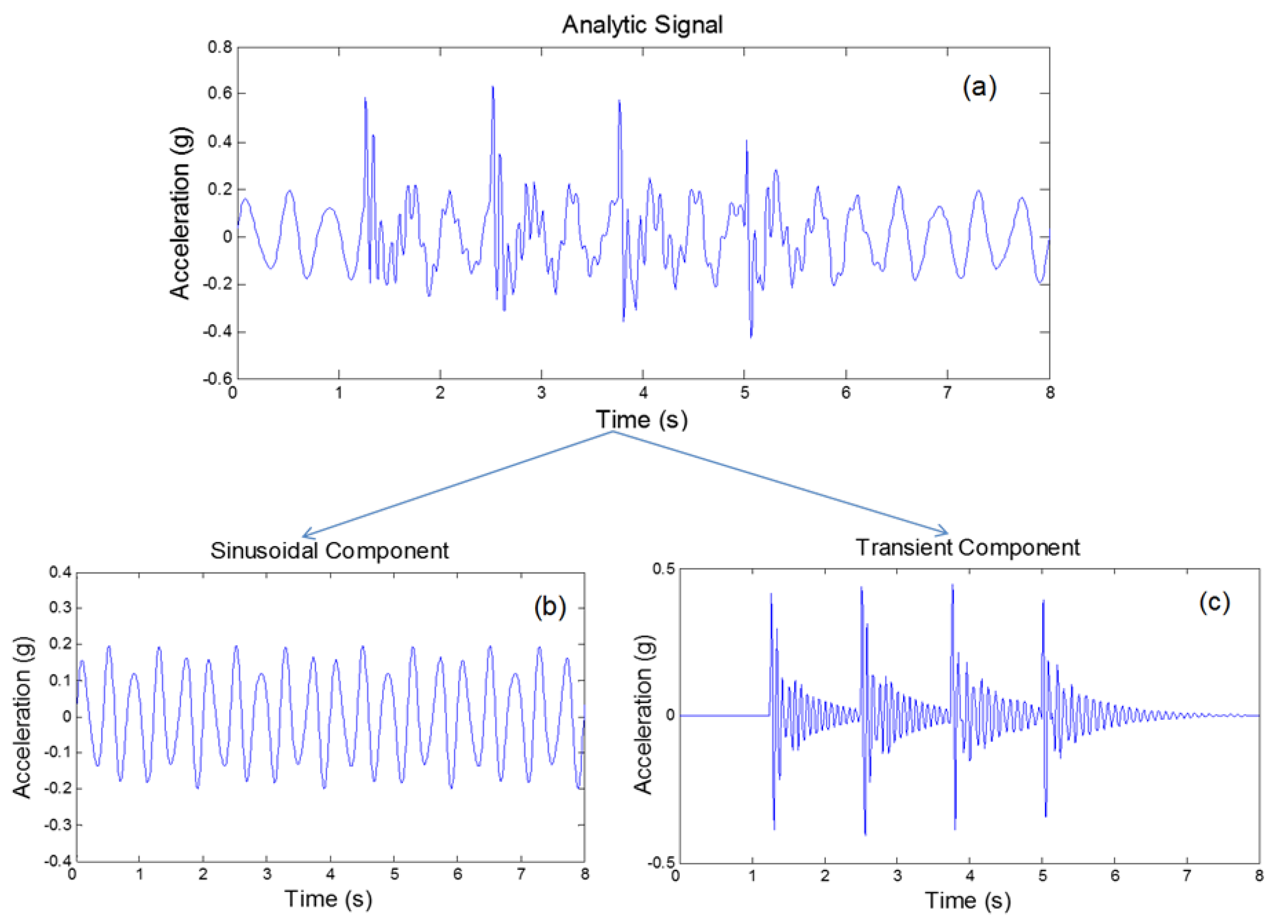
To systematically evaluate the robustness of the SVM algorithm, the signals that mimic realistic dynamic and static signals were considered. For static signals (lying, or sitting, or standing still), the ideal signal remains at zero for the accelerometer and gyroscope for the dynamic signals (normal walking), a nonstationary test signal was constructed, as shown in Figure 9.
The test signal consists of two components:
where represents the periodic component in the signal, given by:
where , and represent the amplitude, initial phase and frequency th of the sinusoidal element, respectively. Two frequency components, 2.5 and 4 Hz, were chosen to construct the fundamental periodicity of the test signal. In Table 1, the specific values of the used parameter are shown.
The term represents the transient component in the signal, given by:
where M is the number of motion cycles, and , , , , and are the amplitude, attenuation factor, time-delay, initial phase and frequency of the human activity cycle, respectively. A total of eight elements were used to construct the transient component of the test signal. The specific values of the parameters were determined through the least square error-based curve fitting method, as listed in Table 2.
The function item specified in Equation (22) identifies the point in time at which a transient element occurs, and is defined as:
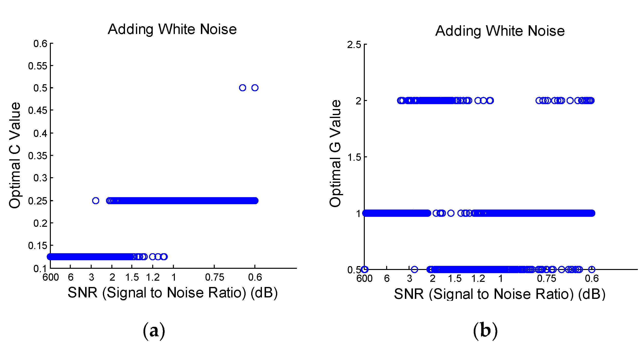
Firstly, the constructed signal was assumed to mimic dynamic activity, and the static activity was represented by zero value from acceleration and angular velocity of all directions. Then, the SVM classifier was utilized to classify the pure simulated dynamic and static activity without any extra noise. We determined that the optimal C value was 0.125 and the optimal G value was 0.5. Subsequently, two different kinds of noise, white and pink noise, were added into the numerically simulated signal with different signal-to-noise ratios (SNRs). The SNR measure in the study was defined as:
where is the power of the signal and is the power of the noise.
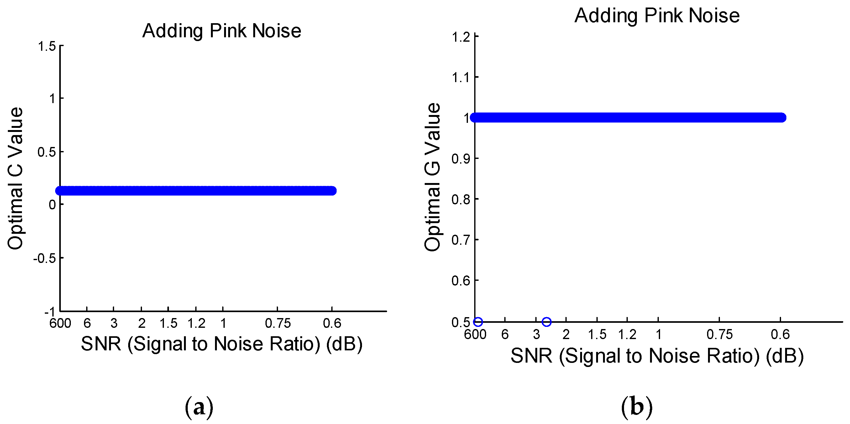
The change of the optimal C and G varied with the change of the SNR level of added white and pink noise, as shown in Figure 10 and Figure 11, respectively. From Figure 10, it can be seen that both C and G change among three different values as the power of added white noise varies. As for the pink noise, Figure 11 shows that C and G almost remain constant, i.e., only a few scattered points are not in the constant line for the optimal G value. The classification accuracy can be maintained at 100% for all these cases, and thus, it shows that the SVM classifier has a good level of capability of processing noisy data due to the adjustment of the optimal parameters.
4. Experimental Results
Classification on Dynamic and Static Activities
As described in the Methodology section, a total of 60 datasets containing 20 dynamic activities and 40 static activities were selected for movement classification; each activity was represented by one two-second data segment. All the datasets were split into training datasets and test datasets equally. Three different trials were performed in the experiment.
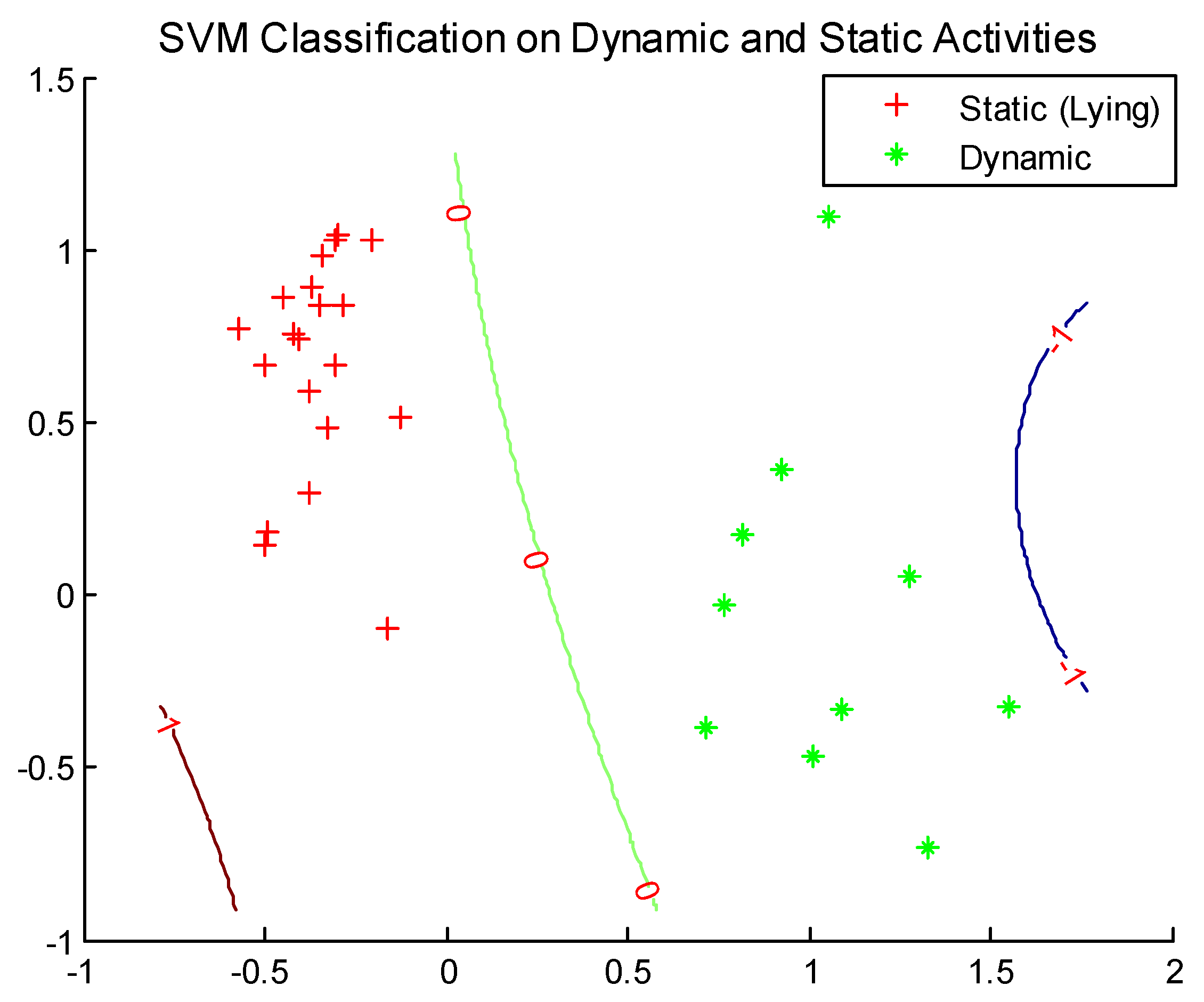
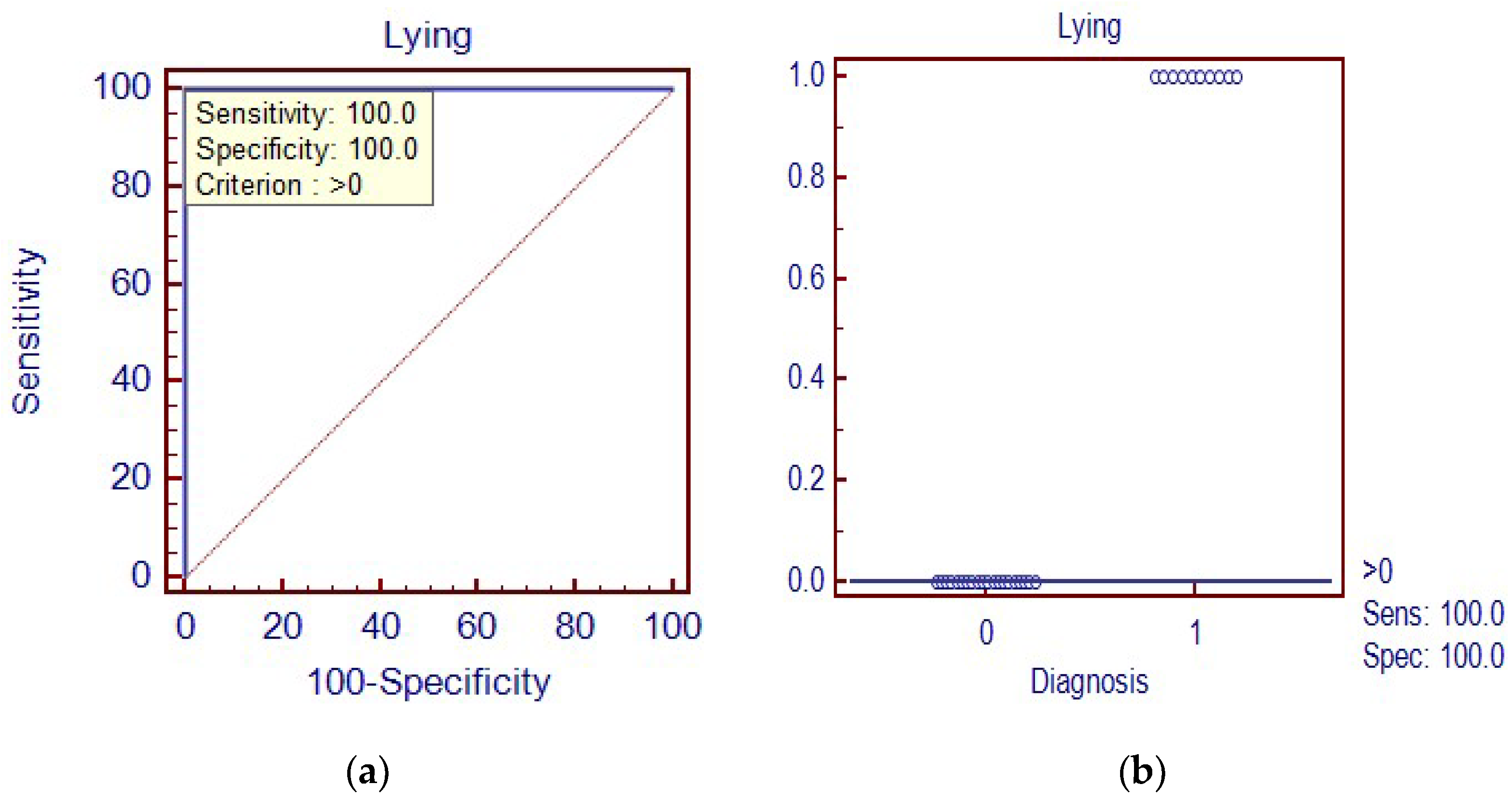
(Walking vs. Lying): 20 normal walking segments were chosen as dynamic activities, and 40 lying segments were chosen as static activities. The datasets were then divided into a training and testing set, each containing 10 dynamic activities and 20 static activities. The 5-fold cross validation scheme [34] was utilized, and 100% (30/30) overall accuracy was observed (classification results are illustrated in Figure 12).
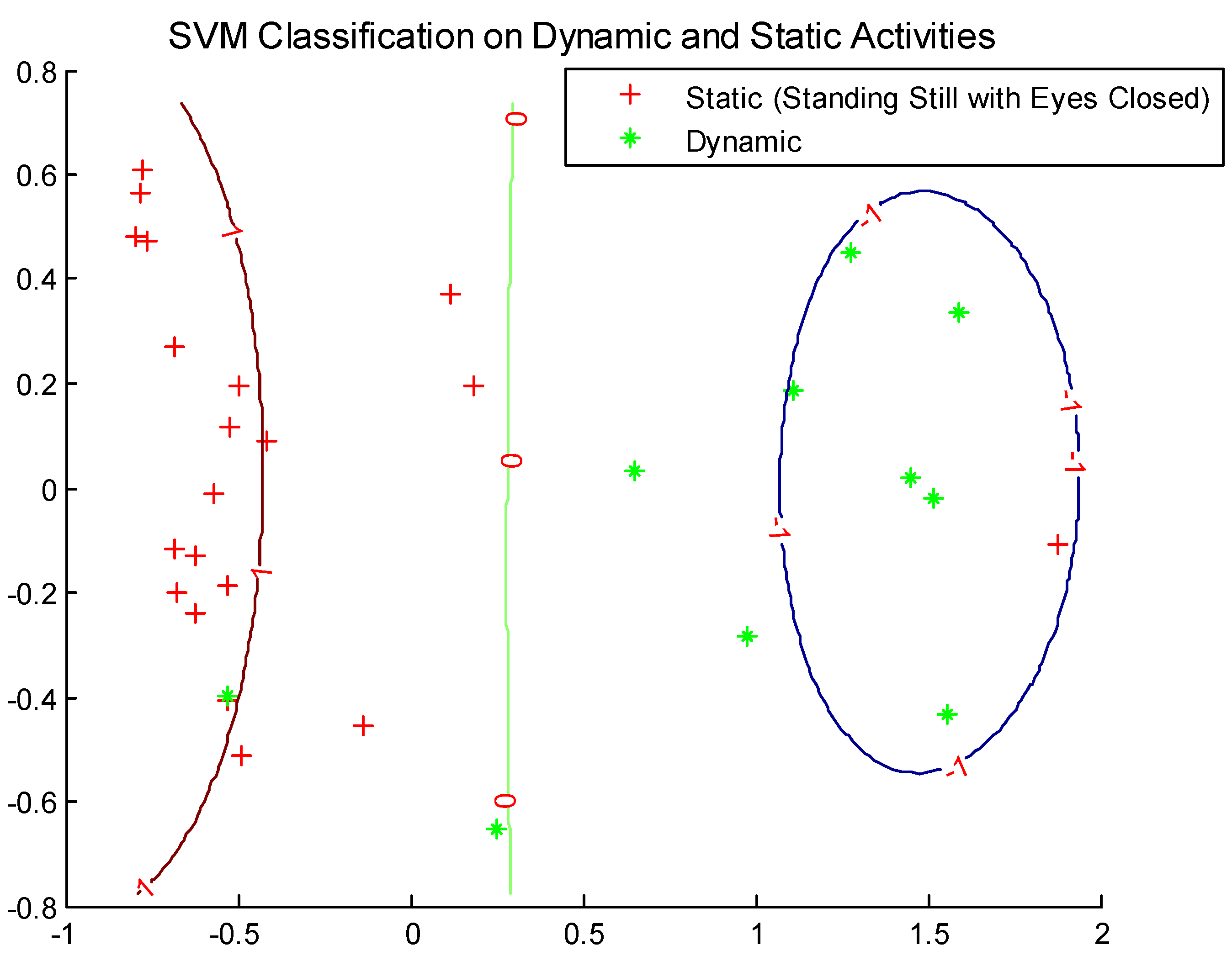
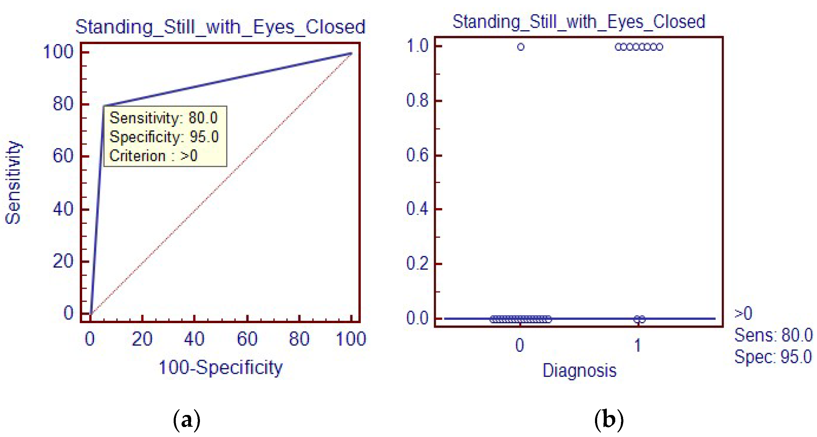
(Walking vs. Standing with Eyes Closed): 20 normal walking segments were chosen as dynamic activities, and 40 standing still with eyes closed segments were chosen as static activities. The same procedure was conducted as the first trial, and 90% (27/30) overall accuracy was observed (the results are illustrated in Figure 13).
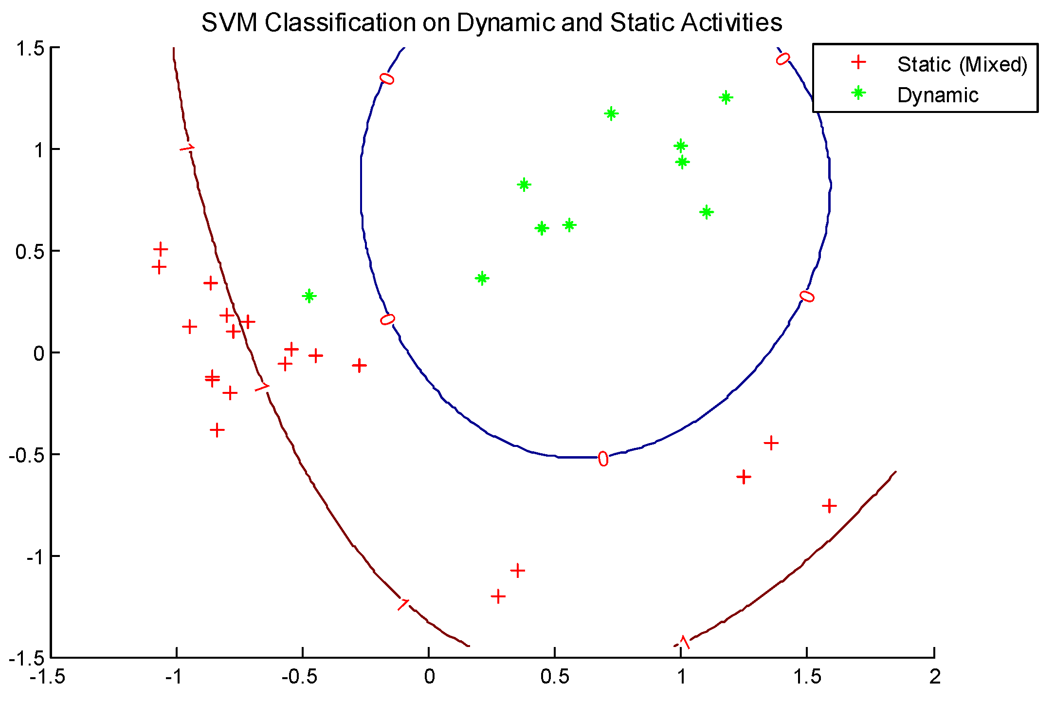
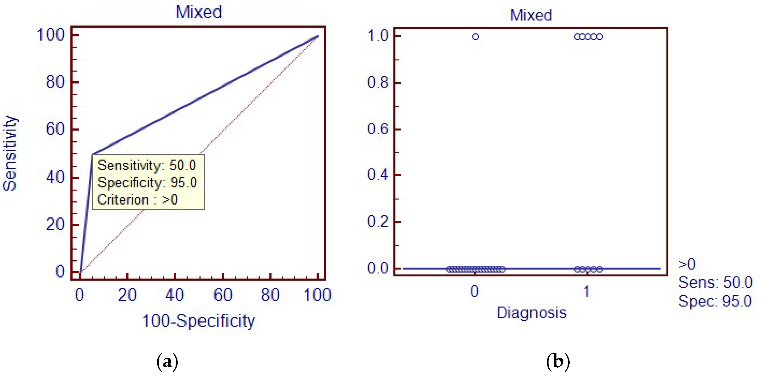
(Walking vs. Lying, Sitting, Standing with Eyes Open and Closed): 20 normal walking segments were chosen as dynamic activities, and four different activities, i.e., lying, sitting, standing still with eyes open and closed, were selected as static activities. Each of them was assigned 10 segments; thus, in total, there were 40 static activities. In this case, we obtained an overall accuracy of 80% (24/30), as shown in Figure 14. Additionally, the corresponding optimal C and values, and the overall classification accuracy associated with sensitivity and specificity, are listed in Table 3.
The sensitivity and specificity of the trials are illustrated in the ROC curves (Figure 15, Figure 16 and Figure 17). The results were consistent with the classification accuracy results. The first trial showed the highest sensitivity value among these three trials, and the third trial had the least sensitivity. In these three trials, the SVM classifier’s sensitivity values were 100.0, 90.0 and 50.0, and the specificity values were 100.0, 95.0 and 95.0. The AUC values for SVM classifier were 1.000, 0.875 and 0.725, respectively.
5. Discussion
This paper mainly aimed to introduce a machine learning technique to biomedical engineers to classify two different states, and to investigate variations in the optimal parameters involved in the SVM algorithm, i.e., C and , as well as the applicability of SVM as a machine classifier to distinguish dynamic and static activities of the older adults using a wearable sensor. The performance of the SVM classifier was investigated in the environment of movement variations. As the performance of different classifiers could be assessed by modulating the movement/noise conditions [42,43], this paper utilized white and pink noise to create a noisy environment in order to evaluate the classification capability of the SVM classifier. In the numerical simulation, both training and test sets were contaminated by white and pink noise; however, the SVM classifier could still stably maintain high classification accuracy by optimizing parameters C and G. Previous studies have reported that C and G could modulate themselves for noisy data [43,44], which is in agreement with our analytic results.
Moreover, this paper examined three different movement variations of static and dynamic activities of the older adults. The results indicated that overall accuracy was optimized by modulating C and for the varied motion patterns, and highest when two activities differed in movement magnitude and direction, such as walking vs. lying still. For example, lying posture is distinguished from other activities by considering the orientation of the accelerometer concerning the direction of gravitational acceleration [45,46] and the intensity of movement [47]. As such, automatic classification of these two motion patterns with a single IMU can be realized with a high level of accuracy using the SVM classifier. Next, comparing walking with standing still, although the direction of the gravitational acceleration remained the same, the activity level may have been different and influenced the boundaries/accuracies. In other words, swaying the whole-body center-of-mass during standing as compared to lying down [45] may have influenced the overall classification accuracy. A mixture of movement variants in terms of the static activities (lying, sitting, standing with eyes open and closed) compared to walking was the least accurate among the comparisons. Although these comparisons were somewhat elementary, the SVM classifier’s performance compared favorably with previous results/studies. For example, Aminian et al. utilized two kinematic sensors (attached to the chest and thigh) to achieve an overall classification accuracy of 89.3% [48]. Busser et al. employed a similar system to achieve an overall classification accuracy ranging between 76% and 92% [49].
Limitations: Conclusions based on this study should be considered in the context of its limitations. First, only a small number of participants were tested, and the results may not reflect the general population of the older adults [44,50,51]. Second, only the steady state motion patterns without transitions were extracted and analyzed. Thus, in order to continuously classify motion patterns using real-time data, the transitional components such as sit-to-stand-walk should be considered further in future research. Third, only the Gaussian kernel function was applied in this work; other factors affecting the optimization of SVM algorithm, e.g., the type and size of the data, the selection of the kernel function, computational cost, etc., should all be considered in future research work. Only limited features were extracted and utilized to distinguish dynamic and static activities; other potentially representative features should be further explored. Despite all of these limitations, however, we believe that SVM is capable of classifying dynamic and static activities of varied motion patterns of the older adults.
6. Conclusions
The SVM algorithm was investigated for classification accuracy. Two parameters that affect the performance of the SVM algorithm—the soft margin constant C, and the other parameter reflecting the kernel function —were systematically investigated. From the simulation results, we can conclude that SVM classifier has the power to classify noisy data. The present study demonstrates the potential of SVM classifier to detect and classify dynamic and static motion patterns of the older adults utilizing an IMU. Although implicated, future studies investigating the transitional aspects of movement variations are required to fully classify dynamic and static motion patterns using SVM classifier.
Author Contributions
J.Z., R.S. and T.E.L. conceived and designed the experiments; R.S. and J.Z. performed the experiments; R.S. along with J.Z. analyzed the data wrote the manuscript with support from T.E.L. All authors have read and agreed to the published version of the manuscript.
Funding
This research was supported by the NSF-Information and Intelligent Systems (IIS) and Smart and Connected Health (1065442, and 1547466, and secondary 1065262).
Acknowledgments
We would like to thank Misha Pavel and Wendy Nilsen for their encouragement in the development of wireless health monitoring systems and fostering the support of wearable wireless health monitoring systems.
Conflicts of Interest
The authors declare no conflict of interest.
References
- Lockhart, T.E. Fall accidents among the elderly. In International Encyclopedia of Ergonomics and Human Factors, 2nd ed.; Karwowski, W., Ed.; CRC Press: Baton Rouge, FL, USA, 2007. [Google Scholar]
- Lockhart, T.E.; Smith, J.K.; Woldstad, J.C. Effects of aging on the biomechanics of slips and falls. Hum. Factors 2005, 47, 708–729. [Google Scholar] [CrossRef] [PubMed] [Green Version]
- Kannus, P.; Sievanen, H.; Palvanen, M.; Jarvinen, T.; Parkkari, J. Prevention of falls and consequent injuries in elderly people. Lancet 2005, 366, 1885–1893. [Google Scholar] [CrossRef]
- Liu, J.; Lockhart, T.E. Age-related joint moment characteristics during normal gait and successful reactive recovery from unexpected slip perturbations. Gait Posture 2009, 30, 276–281. [Google Scholar] [CrossRef] [PubMed] [Green Version]
- Parijat, P.; Lockhart, T.E. Effects of quadriceps fatigue on the biomechanics of gait and slip propensity. Gait Posture 2008, 28, 568–573. [Google Scholar] [CrossRef] [PubMed] [Green Version]
- Liu, J.; Lockhart, T.E.; Jones, M.; Martin, T. Local dynamic stability assessment of motion impaired elderly using electronic textile pants. IEEE Trans. Autom. Sci. Eng. 2008, 5, 696–702. [Google Scholar] [PubMed] [Green Version]
- Oberg, T.; Karsznia, A.; Oberg, K. Joint angle parameters in gait: Reference data for normal subjects 10–79 years of age. J. Rehabil. Res. Dev. 1994, 31, 199–213. [Google Scholar]
- Oberg, T.; Karsznia, A.; Oberg, K. Basic gait parameters: Reference data for normal subjects 10–79 years of age. J. Rehabil. Res. Dev. 1993, 30, 210–223. [Google Scholar]
- Owings, T.M.; Grabiner, M.D. Step width variability, but not step length variability or step time variability, discriminates gait of healthy young and older adults during treadmill locomotion. J. Biomech. 2004, 37, 935–938. [Google Scholar] [CrossRef]
- Hausdorff, J.M.; Rios, D.A.; Edelberg, H.K. Gait variability and fall risk in community-living older adults: A 1-year prospective study. Arch. Phys. Med. Rehabil. 2001, 82, 1050–1056. [Google Scholar] [CrossRef]
- Najafi, B.; Aminian, K.; Loew, F.; Blanc, Y.; Robert, P.A. Measurement of stand-sit and sit-stand transitions using a miniature gyroscope and its application in fall risk evaluation in the elderly. IEEE Trans. Biomed. Eng. 2002, 49, 843–851. [Google Scholar] [CrossRef]
- Lee, M.; Roan, M.; Smith, B.; Lockhart, T.E. Gait analysis to classify external load conditions using linear discriminant analysis. Hum. Mov. Sci. 2009, 28, 226–235. [Google Scholar] [CrossRef] [PubMed] [Green Version]
- Chessa, S.; Knauth, S. Evaluating AAL systems through competitive benchmarking-indoor localization and tracking. In Proceedings of the International Competition, EvAAL 2011, Valencia, Spain, 25–29 July 2011. [Google Scholar]
- Cvetković, B.; Kaluža, B.; Gams, M.; Luštrek, M. Adapting activity recognition to a person with Multi-Classifier Adaptive Training. J. Ambient Intell. Smart Environ. 2015, 7, 171–185. [Google Scholar] [CrossRef]
- Kerdegari, H.; Mokaram, S.; Samsudin, K.; Ramli, A. A pervasive neural network based fall detection system on smart phone. J. Ambient Intell. Smart Environ. 2015, 7, 221–230. [Google Scholar] [CrossRef]
- Curtis, D.; Bailey, J.; Pino, E.; Stair, T.; Vinterbo, S.; Waterman, J.; Shih, E.; Guttag, J.; Greenes, R.; Ohno-Machado, L. Using ambient intelligence for physiological monitoring. J. Ambient Intell. Smart Environ. 2009, 1, 129–142. [Google Scholar] [CrossRef]
- Begg, R.K.; Palaniswami, M.; Owen, B. Support vector machines for automated gait classification. IEEE Trans. Biomed. Eng. 2005, 52, 828–838. [Google Scholar] [CrossRef]
- Chapelle, O.; Haffner, P.; Vapnik, V.N. Support vector machines for histogram-based classification. IEEE Trans. Neural Netw. 1999, 10, 1055–1064. [Google Scholar] [CrossRef]
- Begg, R.K.; Kamruzzaman, J. A machine learning approach for automated recognition of movement patterns using basic, kinetic and kinematic gait data. J. Biomech. 2005, 38, 401–408. [Google Scholar] [CrossRef]
- Lau, H.; Tong, K.; Zhu, H. Support vector machine for classification of walking conditions of persons after stroke with dropped foot. Hum. Mov. Sci. 2009, 28, 504–514. [Google Scholar] [CrossRef]
- Levinger, P.D.; Lai, T.H.; Begg, R.K.; Webster, K.E.; Feller, J.A. The application of support vector machine for detecting recovery from knee replacement surgery using spatio-temporal gait parameters. Gait Posture 2009, 29, 91–96. [Google Scholar] [CrossRef]
- Vapnik, V.N. An overview of statistical learning theory. IEEE Trans. Neural Netw. 1999, 10, 1055–1064. [Google Scholar] [CrossRef] [Green Version]
- Janssen, D.; Schollhorn, W.I.; Newell, K.M.; Jager, J.M.; Rost, F.; Vehof, K. Diagnosing fatigue in gait patterns by support vector machines and self-organizing maps. Hum. Mov. Sci. 2011, 30, 966–975. [Google Scholar] [CrossRef] [PubMed]
- Vapnik, V.N. Statistical Learning Theory; Wiley: New York, NY, USA, 1998. [Google Scholar]
- Vapnik, V.N.; Golowich, S.E.; Smola, A. Support vector method for function approximation regression, estimation, and signal processing. In Advances in Neural Information Processing Systems; MIT Press: Cambridge, UK, 1997; Volume 9, pp. 281–287. [Google Scholar]
- Nuryani, N.S.; Ling, S.H.; Nguyen, H.T. Electrocardiographic signals and swarm-based support vector machine for hypoglycemia detection. Ann. Biomed. Eng. 2012, 40, 934–945. [Google Scholar] [CrossRef] [PubMed]
- Weston, J.; Mukherjee, S.; Chapelle, O.; Pontil, M.; Poggio, T.; Vapnik, V.N. Feature selection for SVMs. In Advances in Neural Information Processing Systems; MIT Press: Cambridge, UK, 2000; Volume 13, pp. 668–674. [Google Scholar]
- Widodo, A.; Yang, B. Support vector machine in machine condition monitoring and fault diagnosis. Mech. Syst. Signal. Process. 2007, 21, 2560–2574. [Google Scholar] [CrossRef]
- Vapnik, V.N. The Nature of Statistical Learning Theory; Springer: New York, NY, USA, 1995. [Google Scholar]
- Cucker, F.; Smale, S. On the mathematical foundations of learning. Bull. Am. Math. Soc. 2001, 39, 1–49. [Google Scholar] [CrossRef] [Green Version]
- Cristianini, N.; Shawe-Taylor, J. An Introduction to Support Vector Machines and other Kernel-Based Learning Methods; Cambridge University Press: Cambridge, UK, 2000. [Google Scholar]
- Barth, A.T.; Hanson, M.A.; Powell, H.C.; Lach, J. TEMPO 3.1: A body area sensor network platform for continuous movement assessment. In Proceedings of the 6th International Workshop on Wearable and Implantable Body Sensor Networks, Berkeley, CA, USA, 3–5 June 2009; pp. 71–76. [Google Scholar]
- Soangra, R. Understanding Variability in Older Adults Using Inertial Sensors. Ph.D. Thesis, Virginia Tech, Blacksburg, VA, USA, 2014. Available online: https://vtechworks.lib.vt.edu/handle/10919/49248 (accessed on 28 July 2020).
- Bouten, C.V.; Koekkoek, K.T.; Verduin, M.; Kodde, R.; Janssen, J.D. A triaxial accelerometer and portable data processing unit for the assessment of daily physical activity. IEEE Trans. Biomed. Eng. 1997, 44, 136–147. [Google Scholar] [CrossRef] [PubMed] [Green Version]
- Chang, C.C.; Lin, C.J. LIBSVM: A library for support vector machines. Acm Trans. Intell. Syst. Technol. 2011, 2, 1–27. [Google Scholar] [CrossRef]
- Jolliffe, I.T. Principal Component Analysis; Springer: New York, NY, USA, 2002. [Google Scholar]
- Gorban, A.; Kegl, B.; Wunsch, D.; Zinovyev, A. Principal Manifolds for Data Visualization and Dimension Reduction; Springer: Berlin/Heidelberg, Germany; New York, NY, USA, 2007. [Google Scholar]
- Mallat, S. A Wavelet Tour of Signal Processing; Academic Press: Cambridge, MA, USA, 1999. [Google Scholar]
- Huang, N.E.; Zheng, S.; Steven, R. The empirical mode decomposition and the Hilbert spectrum for nonlinear and non-stationary time series analysis. Proc. R. Soc. Lond. 1998, 454, 903–995. [Google Scholar] [CrossRef]
- Zhang, J.; Yan, R.; Gao, R.X.; Feng, Z. Performance enhancement of ensemble empirical mode decomposition. Mech. Syst. Signal. Process. 2010, 24, 2104–2123. [Google Scholar] [CrossRef]
- Hudgins, B.; Parker, P.; Scott, R.N. A new strategy for multifunction myoelectric control. Biomed. Eng. IEEE Trans. 1993, 40, 82–94. [Google Scholar] [CrossRef]
- Luukka, P.; Lampinen, J. Differential evolution classifier in noisy settings and with interacting variables. Appl. Soft Comput. 2011, 11, 891–899. [Google Scholar] [CrossRef]
- Nettleton, D.; Orriols-Puig, A.; Fornells, A. A study of the effect of different types of noise on the precision of supervised learning techniques. Artif. Intell. Rev. 2010, 33, 275–306. [Google Scholar]
- Trafalis, T.B.; Alwazzi, S.A. Support vector machine classification with noisy data: A second order cone programming approach. Int. J. Gen. Syst. 2010, 39, 757–781. [Google Scholar] [CrossRef]
- Ng, A.V.; Kent-Braun, J.A. Quantitation of lower physical activity in persons with multiple sclerosis. Med. Sci. Sports Exerc. 1997, 29, 517–523. [Google Scholar] [CrossRef] [PubMed]
- Veltink, P.H.; Bussmann, H.B.J.; de Vries, W.; Martens, W.L.J.; van Lummel, R.C. Detection of static and dynamic activities using uniaxial accelerometers. IEEE Trans. Rehabil. Eng. 1996, 4, 375–385. [Google Scholar] [CrossRef]
- Najafi, B.; Aminian, K.; Paraschiv-lonescu, A.; Loew, F.; Bula, C.J.; Robert, P. Ambulatory system for human motion analysis using a kinematic sensor: Monitoring of daily physical activity in the elderly. IEEE Trans. Biomed. Eng. 2003, 50, 711–723. [Google Scholar] [CrossRef]
- Aminian, K.; Robert, P.; Buchser, E.E. Physical activity monitoring based on accelerometry: Validation and comparison with video observation. Med. Biol. Eng. Comput. 1999, 37, 1–5. [Google Scholar] [CrossRef]
- Busser, H.J.; Ott, J.; van Lummel, R.C.; Uiterwaal, M.; Blank, R. Ambulatory monitoring of children’s activity. Med. Eng. Phys. 1997, 19, 440–445. [Google Scholar] [CrossRef]
- Pashmdarfard, M.; Azad, A. Assessment tools to evaluate Activities of Daily Living (ADL) and Instrumental Activities of Daily Living (IADL) in older adults: A systematic review. Med. J. Islam. Repub. Iran (MJIRI) 2020, 34, 224–239. [Google Scholar]
- Devos, H.; Ahmadnezhad, P.; Burns, J.; Liao, K.; Mahnken, J.; Brooks, W.M.; Gustafson, K. Reliability of P3 Event-Related Potential during Working Memory across the Spectrum of Cognitive Aging. medRxiv 2020. [Google Scholar] [CrossRef]
Figure 1.
Linear support vector machine separation.

Figure 2.
Picture of sensor location on a participant.

Figure 3.
Data analysis procedure.

Figure 4.
Proportion of variance (PoV) curve of the principal components.

Figure 5.
View of the data and the original variables in the space of the first three principal components.
Figure 5.
View of the data and the original variables in the space of the first three principal components.

Figure 6.
The effect of the parameter , on the decision boundary. (a) When = 0.1, the decision boundary is nearly linear. (b) When = 1, the curvature of decision boundary increases. (c) When = 10, the curvature of decision boundary continues increasing, and causes a little overfitting. (d) When = 100, overfitting becomes serious in the classification.

Figure 7.
The effect of the soft-margin constant, C, on the decision boundary. (a) When C = 2, it increases the margin and ignores the data points close to the decision boundary. (b) When C = 200, it decreases the margin and margin error.
Figure 7.
The effect of the soft-margin constant, C, on the decision boundary. (a) When C = 2, it increases the margin and ignores the data points close to the decision boundary. (b) When C = 200, it decreases the margin and margin error.

Figure 8.
Searching the optimal C and value in three-dimension coordinates.

Figure 9.
Test signal generated based on normal walking. (a) Waveform of the test signal ; (b) Periodic component ; (c) Transient component .
Figure 9.
Test signal generated based on normal walking. (a) Waveform of the test signal ; (b) Periodic component ; (c) Transient component .

Figure 10.
(a) Optimal C value for adding white noise; (b) Optimal G value for adding white noise.

Figure 11.
(a) Optimal C value for adding pink noise; (b) Optimal G value for adding pink noise.

Figure 12.
Classification of normal walking and lying activities.

Figure 13.
Classification of normal walking and standing still with eyes closed activities.

Figure 14.
Classification of normal walking and mixed static activities. (Note: Mixed activity in static activities represented by lying, sitting, standing still with eyes open and closed.)
Figure 14.
Classification of normal walking and mixed static activities. (Note: Mixed activity in static activities represented by lying, sitting, standing still with eyes open and closed.)

Figure 15.
ROC curve for classification of normal walking and lying activities. (a) ROC curve; (b) Interactive dot diagram.
Figure 15.
ROC curve for classification of normal walking and lying activities. (a) ROC curve; (b) Interactive dot diagram.

Figure 16.
ROC curve for classification of normal walking and standing still with eyes closed activities. (a) ROC curve; (b) Interactive dot diagram.
Figure 16.
ROC curve for classification of normal walking and standing still with eyes closed activities. (a) ROC curve; (b) Interactive dot diagram.

Figure 17.
ROC curve for classification of normal walking and mixed static activities. (a) ROC curve; (b) Interactive dot diagram.
Figure 17.
ROC curve for classification of normal walking and mixed static activities. (a) ROC curve; (b) Interactive dot diagram.


Table 1.
Parameters related to in the test signal.
| Parameter | Sinusoidal Element (N) | |
|---|---|---|
| 1 | 2 | |
| (V) | 0.16 | 0.04 |
| (Hz) | 2.5 | 4 |
| (rad) | 0 | 0.32 |
Table 2.
Parameters related to in the test signal.
| Transient Component (M) | ||||||||
|---|---|---|---|---|---|---|---|---|
| Group 1 | Group 2 | Group 3 | Group 4 | |||||
| Parameter | 1 | 2 | 3 | 4 | 5 | 6 | 7 | 8 |
| (V) | 0.06 | 0.05 | 0.06 | 0.05 | 0.06 | 0.05 | 0.06 | 0.05 |
| 1.73 | 1.8 | 1.73 | 1.8 | 1.73 | 1.5 | 1.73 | 1.5 | |
| (s) | 1.25 | 1.25 | 2.5 | 2.5 | 3.75 | 3.75 | 5.0 | 5.0 |
| (rad) | 0 | 0.33 | 0 | 0.33 | 0 | 0.33 | 0 | 0.33 |
| (Hz) | 15 | 12 | 15 | 12 | 15 | 10 | 15 | 10 |
Table 3.
Optimal C and values and overall classification accuracy associated with sensitivity and specificity for classifying dynamic and static activities.
Table 3.
Optimal C and values and overall classification accuracy associated with sensitivity and specificity for classifying dynamic and static activities.
| Dynamic | Static | Optimal C Value | Optimal G Value | Overall Classification Accuracy | Sensitivity | Specificity |
|---|---|---|---|---|---|---|
| Normal walking | Lying | 0.25 | 0.1436 | 100% | 100% | 100% |
| Normal walking | Standing still with eyes closed | 0.25 | 0.4353 | 90% | 80% | 95% |
| Normal walking | Mixed activity | 2.2974 | 0.25 | 80% | 50% | 95% |
© 2020 by the authors. Licensee MDPI, Basel, Switzerland. This article is an open access article distributed under the terms and conditions of the Creative Commons Attribution (CC BY) license (http://creativecommons.org/licenses/by/4.0/).
Share and Cite
MDPI and ACS Style
Zhang, J.; Soangra, R.; E. Lockhart, T. Automatic Detection of Dynamic and Static Activities of the Older Adults Using a Wearable Sensor and Support Vector Machines. Sci 2020, 2, 62. https://0-doi-org.brum.beds.ac.uk/10.3390/sci2030062
AMA Style
Zhang J, Soangra R, E. Lockhart T. Automatic Detection of Dynamic and Static Activities of the Older Adults Using a Wearable Sensor and Support Vector Machines. Sci. 2020; 2(3):62. https://0-doi-org.brum.beds.ac.uk/10.3390/sci2030062
Chicago/Turabian StyleZhang, Jian, Rahul Soangra, and Thurmon E. Lockhart. 2020. "Automatic Detection of Dynamic and Static Activities of the Older Adults Using a Wearable Sensor and Support Vector Machines" Sci 2, no. 3: 62. https://0-doi-org.brum.beds.ac.uk/10.3390/sci2030062