Article

Can Shrinking Cities Demolish Vacancy? An Empirical Evaluation of a Demolition-First Approach to Vacancy Management in Buffalo, NY, USA

1
Department of Geography, Texas State University, San Marcos, TX 78676, USA
2
Department of Geography and Planning, SUNY Buffalo State, Buffalo, NY 14222, USA
*
Author to whom correspondence should be addressed.
Submission received: 1 August 2018 / Revised: 10 August 2018 / Accepted: 12 August 2018 / Published: 13 August 2018

Abstract

:
Publicly-funded demolition of vacant structures is an essential tool used in shrinking cities to eliminate nuisances and, often, reduce vacancy rates. Concerning the latter, however, when shrinking cities implement large-scale demolition programs independent of complementary planning efforts, it is reasonable to expect impacts on vacancy to be negligible. Among other reasons, demolition operates only on the outflow of existing vacant structures and largely fails to grapple with inflows that add to vacancy over time. This article evaluates an ambitious demolition program in Buffalo, NY, USA, that sought, explicitly, to lower the municipality’s overall vacancy rate. Evidence from statistical changepoint models and Granger tests suggest that, while Buffalo’s overall vacancy rate, measured as undeliverable postal addresses, appeared to decrease around the time of the program, the drop was not linked to elevated demolition activity. The same finding holds for the subarea in which demolitions were spatiotemporally clustered. Although this lack of efficacy is potentially because the city failed to demolish its targeted number of structures, we argue that the likelier explanation is that demolition was not part of a holistic planning strategy. These results have important implications for using large-scale demolition programs as standalone vacancy management policies in shrinking cities.

1. Introduction

Across the Global North, “shrinking cities” [1], alternatively termed legacy cities or cities in transition [2,3], are a cohort of older urban settlements that once played prominent roles in the industrial economy but, in the second half of the 20th century, experienced persistent, prevalent, and severe depopulation, economic contraction, and undesirable physical change [1,4,5,6,7,8]. In the American experience, post-World War II federal highway and mortgage lending policies enabled mass suburbanization by pushing relatively affluent residents from central cities toward rapidly developing adjacent suburbs [9,10]. Happening at and around the same time was a massive drop-off in local manufacturing and industrial production that saw factories, mills, and warehouses close, leaving scores of urban residents without jobs [8]. Many former workers left industrial cities and regions altogether to seek employment elsewhere. The cumulative results of these and connected push-and-pull forces, in addition to natural demographic change [5], have left American cities such as Buffalo, NY; Cleveland, OH; Detroit, MI; Pittsburgh, PA; and St. Louis, MO; among others, with less than half of their peak populations [4].
One consequence of massive population loss is that the built environments of shrinking cities, which were constructed for multiples of their current (post-shrinkage) commercial and residential populations, become dotted with ever-increasing inventories of vacant and abandoned structures [11]. Vacant and abandoned properties are significant obstacles to neighborhood and city stabilization, reinvestment, and revitalization [12], insofar as they tend to reduce nearby property values and contribute to the geographic diffusion of blight [13]. As such, vacancy and abandonment are popular, and necessary, targets for public policy intervention in shrinking cities [14]. At least in the United States, however, decision-makers in shrinking cities regularly conceptualize these phenomena as relatively static in nature, and, for that reason, largely eradicable through public spending on structural demolitions and public policies that are friendly to economic development and oriented toward re-growth (e.g., [15]). Yet, as ample scholarship on shrinking cities tends to agree: (1) the problems related to urban shrinkage and decline are manifold and complex (e.g., [16,17,18]), which suggests that simply demolishing existing vacant and abandoned structures is unlikely to correct the issue; (2) demand for housing in shrinking cities is often very weak and highly spatially uneven, such that neighborhoods with excessive vacant housing stocks and related conditions of urban decline rarely benefit from the limited growth or development that does occur in shrinking cities [3,19]; and, (3) at bottom, the pro-growth mental model underlying many policy programs in shrinking cities rests on assumptions of re-growth that are rarely grounded in the reality of the cities’ current circumstances or near-term prospects [15].
While there are certainly counter-examples pushing against the broad strokes painted in the preceding paragraph (e.g., [20,21,22]), the literature and recent historical record suggest that pro-examples are much more numerous (e.g., [8,15,16,23,24,25]). In one case that is relatively popular among American shrinking cities researchers (e.g., [15,26,27,28,29,30,31,32,33]), the “5 in 5” demolition program enacted in 2007 in Buffalo, NY, USA, famously sought to demolish 5000 vacant and abandoned properties over five years, in an attempt to bring the city’s overall “vacancy rate … closer to five percent”, down from the estimated citywide vacancy rate of 15 percent at the policy’s inception [34] (pp. 1–2). Ultimately, the city fell short of its ambitious 5000 demolition target due to financial constraints, which calls the program’s efficacy into question [15] (p. 9). Crucially, though, we argue that it was the city’s logic, especially the assumption that demolishing a specific quota of vacant and abandoned properties can materially and unilaterally affect a shrinking city’s overall vacancy rate, and not financial infeasibility per se that was the fatal flaw of the “5 in 5” program. We make the case that similar logic will continue to undermine any vacancy management strategy that fails to grapple with the complexity and dynamism of urban shrinkage and decline (see related arguments in [8,11,15,27]). To aid us in building that case, we undertake an empirical evaluation of Buffalo’s “5 in 5” program directed at the following questions:
  • Where did demolitions occur around the time of the “5 in 5” program, and was Buffalo’s demolition activity spatiotemporally clustered in any subareas of the city? (NB: if clusters are detected, then we will seek to answer questions #2–4, below, at both the citywide/global and cluster-area/local levels of analysis. This multi-scalar approach will be taken to account for the possibility that the program’s efficacy might look different in the subarea(s) where it was most active relative to the city as a whole.)
  • Did vacancy in the study area(s) appear to change significantly around or since the time of the “5 in 5” program?
  • Did demolition activity in the study area(s) appear to change significantly around the time of the “5 in 5” program?
  • Does demolition activity in the study area(s) Granger-cause changes in vacancy? (where Granger causality describes a statistical test used to detect the extent to which one time series influences [“Granger-causes”] a second time series). For this question, we are interested in knowing whether the “5 in 5” program’s foundational premise—that more demolitions can cause change to Buffalo’s vacancy stock—holds up when placed under an empirical microscope. Null findings here would support our contention that demolition alone does not offer a simple solution to complex vacancy problems in shrinking cities. As such, this fourth question is the one in which we are most interested. Answers to questions #1–3 guide our approach to answering this core question, as well as inform our interpretation of results.
Prior to describing the materials and methods used to answer these questions, the remainder of this section frames our intervention and briefly characterizes its place in the shrinking cities literature. In doing so, we start from the foundation that problems related to urban decline are interdependent and multi-causal [16]. For that reason, to more effectively manage these problems, political decision-makers must replace simple, event-oriented thinking (e.g., “if we demolish more structures, then the vacancy rate will necessarily fall”) with more complex, systems thinking that appreciates feedback effects and opens the door for comparatively proactive strategies that are grounded in real world circumstances, patterns, trends, and possible futures. With respect to the case under investigation—Buffalo’s “5 in 5” demolition program—we produce empirical evidence to suggest that demolition by itself has limited efficacy for substantively changing vacancy in a shrinking city. These results buttress the argument that cities ought to avoid using demolition as a standalone vacancy management strategy, and must instead incorporate it into longer-term, multi-pronged, holistic approaches [2,14,35,36,37]. Importantly, in framing the empirical analyses, we draw heavily from the toolbox of systems thinking. Employing these tools allows us to interpret our results in a way that offers several important lessons for practitioners in shrinking cities. Above all, our discussion challenges decision-makers to enumerate the relevant (known) sources of change that affect a given variable (e.g., vacancy) prior to designing an intervention aimed at altering that variable. Part of that exercise, as we illustrate, must involve identifying and critically engaging with the core assumptions, or “mental models”, that underlie the desired intervention.

1.1. On Shrinkage, Decline, and Their Causes and Symptoms: A Brief Introduction

Cities are complex systems made up of untold numbers of interacting parts [38]. When a shock affects one or more of those parts in space and time, the interconnectivity of the system’s parts and subsystems implies that consequences can be many orders of magnitude greater than the original shock [39]. That is, changes in any part of an interconnected urban system can give rise to powerful self-reinforcing feedback processes.
Prior to World War II, these feedback processes almost unanimously pointed to a virtuous cycle of urbanization. Simply put, cities grew. The world over, prewar industrialized cities enjoyed steady, positive inflows of people, jobs, aggregate income, and built structures [40]. Indeed, the field of urban planning emerged largely from the need to control and manage these widespread, seemingly unabating patterns of city growth [9]. While urban growth did not stop after World War II (in fact, the urban share of global population has increased in every decade since 1940 [41]), by 1950 the phenomenon became far narrower in its geographical scope. That is, whereas prewar urbanization was mostly distributive, in that it seemingly applied to all cities, postwar urbanization has been comparably parasitic, fueling growth in some cities while contributing to stagnation, shrinkage, and/or decline in others [4].
Acknowledging that there is no universally accepted definition of the concept [6], elsewhere in our work [8] we have interpreted shrinkage as sustained, downward, quantitative adjustments to the population of a geographic community (also see [27]). Stated another way, urban shrinkage involves long-term, “persistent” decreases in the total number of people living in an affected, shrinking area [40]. Frequently, this sort of sustained population loss is accompanied, preceded, and/or succeeded by downward quantitative adjustments (shrinkage) in the size of the economy and built environment of the depopulating community. In other words, population loss tends to be highly correlated with both (1) job loss and (2) vacancy and property abandonment, the latter of which precedes property demolition [8]. While the precise chain of causality involved in this complex relationship remains unresolved [5], most researchers and practitioners agree that these linkages between population, the economy, and the built environment mean that shrinkage, decline, and their many manifestations cannot possibly have simple, standalone policy fixes [16,17].
On that backdrop, unlike the predominantly virtuous cycles of prewar distributive urbanization, the contemporary era of parasitic urbanization has placed numerous shrinking communities across the world into vicious cycles of harmful, self-reinforcing demographic, economic, and physical change. These quantitative decreases are much more than accounting matters. As American urban scholar Lewis Mumford observed in The City in History [42] (p. 486), these changes often lead to a “breakup of the old urban form”. That is, parasitic urbanization tends to have deleterious effects on a shrinking city’s existing urban functions. Through that lens, distinct from quantitative shrinkage, we interpret decline as negative qualitative change to the fabric and form of a given geographic community. Following basic dictionary definitions of the words “fabric” and “form”, urban fabric is taken to mean the comprehensive collection of a community’s social and physical elements and their spatial arrangement in relation to each other. Furthermore, urban form is interpreted to be the novel structures, such as neighborhoods and patterns of positive or negative social relations, that emerge from localized interactions between elements in the urban fabric (see [43]). In this vein, urban decline is a downgrading in the quality of the urban fabric that can lead to, in the spirit of Mumford’s observation, “breakup” of the existing urban form (e.g., neighborhood abandonment; see [44]).
Based on the foregoing definitions, urban shrinkage can be understood as a sufficient, but not a necessary, condition for urban decline. While the quantitative adjustments related to shrinkage invariably coincide with qualitative change in the urban fabric or form of an affected place [45] (pp. 9–10), the latter phenomena can occur in the absence of the former. That is, decline can take shape in all varieties of communities, regardless of whether their populations are growing, shrinking, or stable. Decline, it follows, has been operating in cities since long before the notion of urban shrinkage came to the attention of academic researchers and planners (e.g., [3]). The significance of this point lies in the fact that shrinkage and decline tend to be conflated in both theory and practice (see [8]). As such, widely adopted policy strategies crafted in response to decline in otherwise growing or stable city contexts, such as government-funded blight removal via structural demolition, followed by opening cleared spaces to private reinvestment [12], are regularly taken up by cities where decline is exacerbated by shrinkage and vice versa [8]. The problem with this approach is that many such policies rest on assumptions about private market demand that do not hold in shrinking cities [3]. More precisely, the problem lies in simplistic event-oriented thinking of the form: “if you clear it (the land), they will come (the real estate developers)”. Thinking more systemically about shrinkage and decline ought to better illuminate the weakness with this type of reasoning. It is on this note that we present and employ two systems thinking tools that the shrinking cities research and practice communities might find valuable for framing problems and crafting solutions.

1.2. Two Systems Thinking Tools for Planning and Decision-Making in Shrinking Cities

1.2.1. The Iceberg Model

Systems thinking is an inquiry-based approach to explaining the relationships between the structures and behaviors of a system [
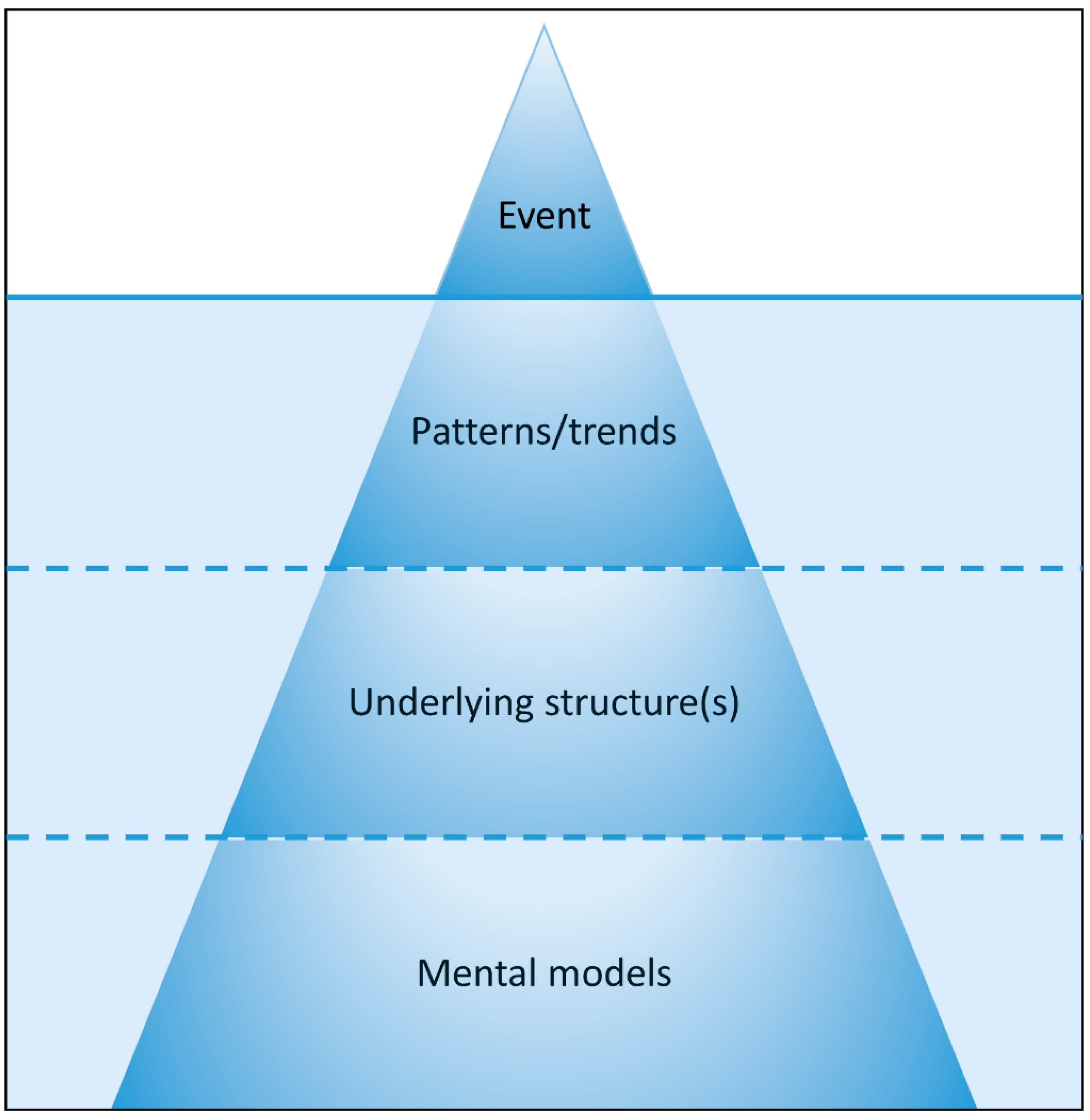
46]. Effective systems thinking requires one to ask probing questions about how the many parts of a system interact and influence one another, and how those part-level interactions have consequences at the level of the whole. In this way, systems thinking endeavors to go “below the surface” to uncover systemic (e.g., structural, cultural, and political) attributes that produce certain patterns and events. One tool for systems thinking is the popular iceberg model [47] depicted in Figure 1.
The iceberg model is a tool for contextualizing a given (observable) problem or event (e.g., vacancy and abandonment) as part of a whole system (e.g., the political economy and prevailing cultural norms of a shrinking city). Like an iceberg, the model imparts that what we see is only a small fraction of the system that produces the observable outcome. The majority of what we would like to know lies beneath the surface [47]. Immediately below the surface, then, is where we might find patterns of behavior in space or time. These patterns or trends in behavior would suggest that the observable problem or event of interest might be part of some larger scope or longer-term tendency. Underlying all patterns or trends is a structure or set of structures from which the observable behavioral patterns are generated. Structures include, among other variables, institutions of governance, their interrelationships, laws and regulations, and, especially, the market-based allocation, production, and consumption mechanisms that prevail in developed nations. Finally, below the structural level are the mental models, i.e., the attitudes, values, beliefs, norms, and conventions, that keep the existing structure(s) in place.
As a tool for facilitating systems thinking, the iceberg model equips its users with at least some capacity to identify leverage points in the system under investigation. Leverage points are places to intervene in the system, where making some sort of strategic modification could nudge the system toward a different, preferably more desirable state [46]. Two generic types of leverage points and interventions implicated by the iceberg model are: (1) redesigning the structure(s) of the system; and (2) transforming mental model(s) in the system [48]. Within the shrinking cities literature, there have been numerous recent calls for decision-makers to supplant growth-oriented goals and their attendant pro-growth policies [9,10,23] with visions of “smart shrinkage” or “right-sizing” [8,9,10,11,27]. In interpreting our results, we suggest that heeding these calls is tantamount to transforming the [pro-growth] mental models that help to create and reinforce patterns of parasitic urbanization [8].

1.2.2. Stock and Flow Diagramming and Feedback Loops

In systems, stocks are inventories that exist at a particular point in time. The sizes of inventories change as a result of flows, or the rates at which units are added to (inflow) and subtracted from (outflow) the stocks over time [46]. The classic example of a stock with one principal inflow and one principal outflow is an unoccupied bathtub. The quantity of water present in the bathtub is the available stock. The water entering the tub through the activated faucet is the inflow that adds to the stock over time, and the quantity of water leaving the tub through an unplugged drain is the outflow that subtracts from the stock. If the inflow and outflow per unit time are equal, then the stock of water remains the same. Discrepancies between the two flows cause the water stock to either increase (when inflow > outflow) or decrease (when inflow < outflow) over time.
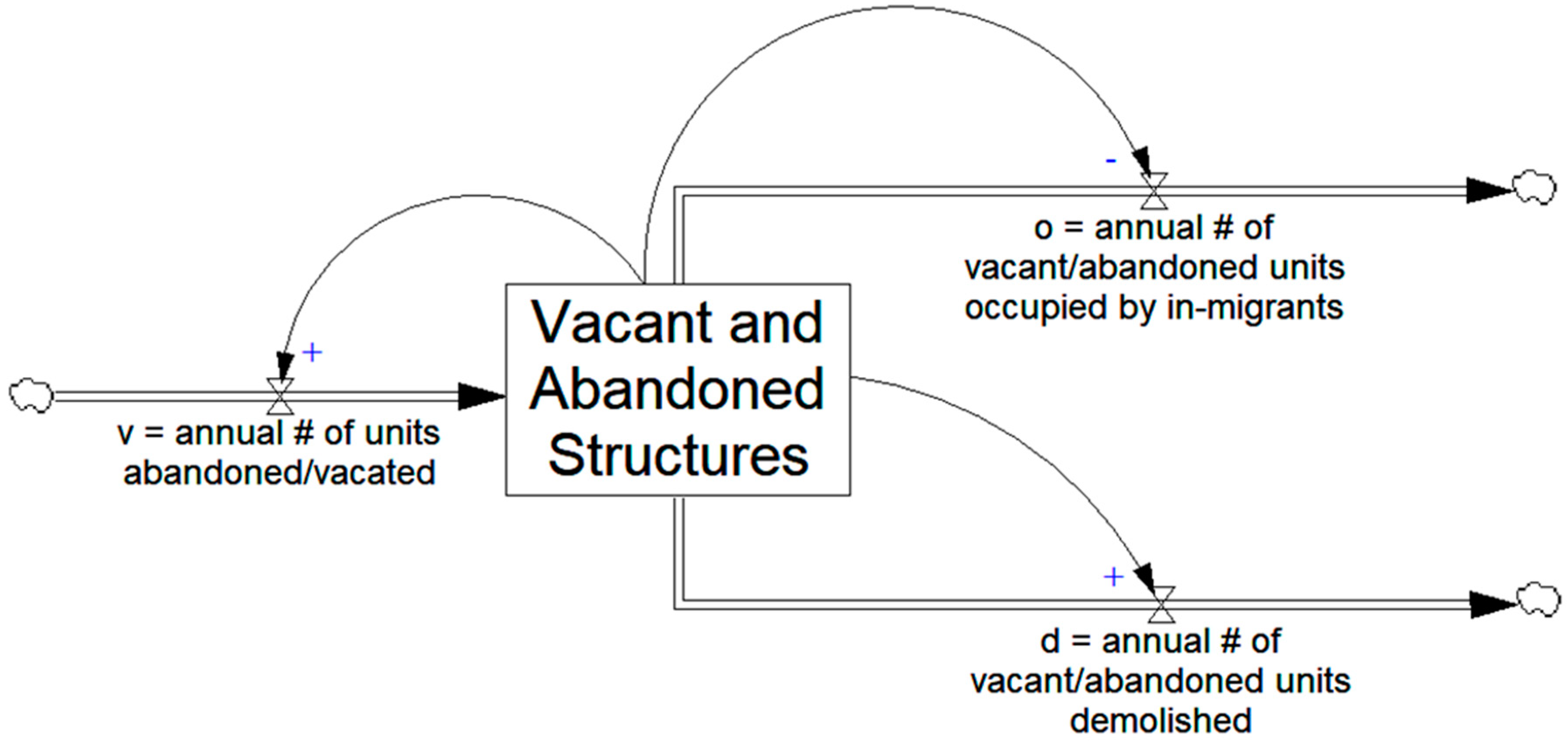
For planning and decision-making purposes, we claim that there is utility in visualizing stocks and flows prior to implementing an intervention that seeks to change one or more of them. Visualizing stocks and flows is called diagramming. Figure 2 presents a simplified stock and flow diagram that considers annual changes to the inventory of vacant and abandoned properties in a city. The large rectangle at the center of the diagram represents the stock of vacant and abandoned properties. Adding to the stock is the annual rate at which properties are vacated and/or abandoned in the city (labeled v in the diagram). Subtracting from the stock are two outflows. First is the annual rate at which vacant and abandoned properties are occupied by in-migrants or otherwise reused (labeled o). Second is the annual rate at which vacant and abandoned properties are demolished or otherwise torn down (d). From year to year, the net effects of these inflows and outflows are responsible for changes measured in the stock of vacant and abandoned structures. When inflows exceed outflows, the vacancy problem worsens. Balanced flows result in a stable or constant stock of vacant and abandoned properties. Furthermore, citywide vacancy is lessened when outflows are collectively larger in magnitude than inflows.
Three feedback loops are depicted in the simplified diagram above. First, research has shown that the more vacant, abandoned, and blighted properties there are in an area, the more likely it is that additional properties fall into disrepair and become abandoned over time (e.g., [13,49]). Stated another way, larger stocks of vacant and abandoned properties often strengthen their own inflow (v). Second, the higher the stock of abandoned or blighted structures in a given area, the lower is the demand for property therein (e.g., [3]). As such, the size of stock shown in Figure 2 affects the rate at which properties are occupied or otherwise reused over time (o). Third, considering evidence that policies aimed at reducing blight are largely reactive [33,37], it is likely the case that larger stocks of vacant and abandoned properties are met with more aggressive levels of publicly funded demolitions (d). Indeed, such a reaction was arguably one of the driving forces behind Buffalo’s “5 in 5” demolition program.
While we turn next to the specifics of that program, it is worth observing here that the stock and flow diagram from Figure 2 provides convenient framing for our empirical analyses, and the iceberg model from Figure 1 provides a medium through which we can interpret our results. Explicitly, Figure 2 makes it clear that the demolition outflow (d) is only one source of change affecting vacant property stocks. Thus, in the absence of complementary policies to balance the remaining two flows (v and o), demolition should not be expected to substantively reduce vacancy (hence our fourth and primary research question from above). With respect to Figure 1, the reason that standalone demolition programs continue to endure as vacancy management strategies in shrinking cities [8,11], despite the logic against such a practice (Figure 2), is perhaps that decision-makers subscribe to pro-growth mental models [9,23] that assume growth is the “natural” urban tendency [5], and that clearing land will necessarily bring new development (and, with it, new demand for urban housing) [8,23].

1.3. The “5 in 5” Demolition Program in Buffalo, NY, USA

In the summer of 2007, facing public and political backlash on the issue of vacancy following life-threatening injuries to a firefighter during a structure fire at an abandoned property, newly-elected Mayor Byron Brown and his administration hurriedly put together a demolition program. In August of that year, a policy brief introduced the program as “Mayor Brown’s ‘5 in 5’ Demolition Plan” [34]. Calling vacancy “one of the most important issues facing our community,” the Mayor’s plan was a highly aggressive program aimed at demolishing 5,000 structures over a five-year period. An explicit goal of the plan was to reduce the number of vacant structures in the city and get the vacancy rate “closer to 5%”, down from the estimated 15% at the time of the policy brief [34]. Past research has criticized the seemingly arbitrary nature of this target [8], as well as the fact that the program mainly functioned outside of larger planning contexts [3,11]. More specifically, while the city’s adopted comprehensive plan included a Vacant Property Asset Management Strategy, the “5 in 5” program conspicuously was not linked to it, calling into question its potential to be successful [27]. Additionally, Yin and Silverman [33] and Silverman et al. [15] have discussed the reactionary nature of the program, arguing that its detachment from proactive and comprehensive planning efforts undermined its efficacy.
In this context, the present paper is not breaking entirely new ground in critiquing the “5 in 5” program. What we add to the discussion, though, is a systems thinking perspective along with novel empirical results. Concerning the former, as expanded on in the next subsection, both the framework of systems thinking and the contents of its toolbox that were introduced above allow us to expose flaws in the program in a way that offers a broad lesson for vacancy management in shrinking cities. In particular, we demonstrate that demolition alone cannot cure vacancy. Whereas existing literature has drawn on observational data and professional insights to make a similar case [3], our approach illustrates, logically, why demolition can only ever be a partial solution to vacancy problems. With respect to the latter contribution, we rely on that same systems thinking framing to guide an empirical evaluation of the “5 in 5” program that moves our critique beyond dialogue (e.g., [11,27]) and into the realm of quantitative evidence.

Challenging the “5 in 5” Program’s Event-Oriented Thinking

Conventional or “event-oriented” thinking assumes that problems are “well bounded, clearly defined, relatively simple and linear with respect to cause and effect”, such that they are solved either “through control of the processes that lead to [them]…or through amelioration of the problem after it occurs” [50] (p. 78). In this sense, problems, or observed events, are the tips of the iceberg from the model shown in Figure 1. Solutions proposed from an event-oriented perspective rarely dig below this surface to reveal the structures or mental models that exist in the system. Instead, the world is thought to function at or near the water line. The “5 in 5” program arguably falls into this trap.
For the “5 in 5” program, the surface-level problem identified by decision-makers was a large stock of vacant and abandoned properties; around 15% of all structures were thought to be vacant, and the city viewed 5% vacancy as a more desirable number. In event-oriented fashion, the city’s proposed solution to the problem was “amelioration” (see [50]) in the form of structural demolitions. The city reasoned that by increasing a known outflow of vacant and abandoned property (Figure 2), the “5 in 5” program would necessarily reduce the stock targeted by the policy. As an example, assume that a city contains 50,000 total structures. With a 15% vacancy rate, the stock of vacant properties in the city would therefore consist of 7500 structures. If 5000 of these structures were demolished and no other changes were made, then the city would be left with 45,000 total structures, 2500 of which would still be vacant, for a 5.6% vacancy rate. In this hypothetical scenario, the “5 in 5” program accomplishes its goal: through aggressive demolition activity, the city’s vacancy rate gets “closer to 5%” from where it was at the inception of the program.
The problem, of course, is that this way of thinking ignores the other flows affecting vacancy (Figure 2). In reality, the social, political, and economic structures of shrinking cities are such that communities become locked into downward spirals, whereby the “spatial-economic” attributes, “social-cultural fabric”, and “image aspects” of cities deteriorate seemingly unabated [16] (p. 1519). In such scenarios, wherein “the young and talented tend to migrate, leaving the elderly and underprivileged behind” [16] (p. 1511), the possibility that annual property abandonment rates and annual reuse/new occupancy rates are fixed to zero or otherwise perfectly counterbalanced (see Figure 2) is far-fetched. Real estate demand in such spaces tends to be weak or non-existent [3], while “push factors”, such as urban blight, inadequate public service provision, and concentrated poverty, continue to incentivize outmigration [16].
On that note, the “5 in 5” program’s key premise—that demolition can unilaterally reduce vacancy stocks—is vastly oversimplified. Without designing additional instruments to influence, at minimum, the city’s rate of property abandonment (v in Figure 2) and/or the rate of property reuse (o in Figure 2), there is no reason to expect relatively non-strategic demolition programs [11,27], no matter how aggressive or large in scope [12], to meaningfully decrease vacant property stocks in shrinking cities. This broad, systems thinking lesson for shrinking cities echoes the chorus of scholars and practitioners who call for demolition programs to be grounded in and guided by comprehensive planning efforts [2,13,35,36,37].
To add empirical support to the claim, below we build up to a test of the null hypothesis that demolition activity does not Granger-cause vacancy rates; in other words, that demolition rates do not influence vacancy over time. We expect this null hypothesis to hold up against the alternative that demolition does in fact influence vacancy on its own. Prior to performing this analytical operation, however, it is worth briefly engaging with the iceberg model of systems thinking (Figure 1) to consider what mental models underlie efforts like the “5 in 5” program, which appears to be guided by unrealistic assumptions.
While we encourage readers to look elsewhere in the literature for deeper dives into the mental models that persist in many shrinking cities (e.g., [16,51]), here it is worth highlighting one. Specifically, as prior research has already pointed out [15], demolition programs are regularly crafted with a pro-growth bias, whereby growth is seen as “success” and shrinkage and decline are framed as “failure” [15] (also see [8,16,23]). Within this mental model, vacant and abandoned properties are typically considered blighting factors and, consequently, hindrances to growth and development (and therefore obstacles to success) [15]. Thus, the logic goes that eradicating blighting factors via structural demolition will remove barriers to growth and development, thereby, seemingly automatically, triggering new development [8]. In other words, based on past urban growth scenarios [4], decision-makers often hold onto the notion that there is an assumed demand for developable land in all cities, including shrinking ones [23]. Once again, this reasoning ignores structural issues that lie below the surface of the problem. Namely, recall that real estate demand in shrinking cities tends to be critically low in most places [3], which implies that blight removal (via demolition) by itself is a poor economic development strategy [8].

1.4. Recap

In summary, urban researchers uniformly agree that shrinkage and decline are complex phenomena with multiple interdependent causes and multiple interdependent consequences (e.g., [5,8,16,39]). As such, an observable problem like a high stock of vacant and abandoned properties cannot be fixed by a single, independent policy instrument such as structural demolition. A systems thinking perspective makes the reason for this outcome clear. Simply put, demolition is only one outflow from a vacant property stock that is affected by at least two other dynamic flows (Figure 2). Without designing programs to account for those other sources of flow, expectations about the capacity for large-scale demolition programs to reduce vacancy stocks should be kept in check.
Related to this point, scholars have critiqued large-scale demolition programs in general [8], and Buffalo’s “5 in 5” demolition program in particular [15], on the grounds that they are typically reactive, disconnected from larger comprehensive planning efforts, and built on a pro-growth mental model containing unrealistic expectations about development potential in shrinking communities [11,15,23,27]. What is still lacking to date, though, is an empirical test of the foundational premise from the “5 in 5” and related programs that demolition alone can decrease vacant property stocks in a shrinking city. While our systems thinking framework casts severe doubt on this proposition, it is important to add empirical weight to the argument. Such is the cause taken up herein.

2. Materials and Methods

To generate answers to the questions posed at the outset of this paper (Section 1), data were obtained from two sources and analytical operations were divided into three phases or sets of tasks. Details on these materials and methods are as follows.

2.1. Data

The two variables implicated in our research questions are demolished and vacant properties. Concerning the former, note that the “5 in 5” demolition program launched in September 2007. Given the program’s temporal mandate, “5 in 5” was therefore set to conclude five years later, at the end of August 2012. In April 2018, we requested a report from the City of Buffalo to cover all completed structural demolitions, regardless of date performed, for which electronic data were available on both: (1) the physical address of the demolished property; and (2) the date on which the demolition was completed. The data provided to us in response to that request was a Microsoft Excel spreadsheet containing 4618 records and covering a time period from October 2005 (the first demolition in that month occurred on 5 October 2005) through the end of 2017 (the final demolition of the year occurred on 20 December 2017). Of those records, 4613 (99.9%) were successfully geocoded on their physical street addresses using the local composite address locator in Esri’s ArcMap 10.5.1. (We retained only point location or street address matches. The five discarded records could only be matched to ZIP code centroids and were therefore deemed unusable.).
With respect to vacancy, the City of Buffalo, like most U.S. cities, does not maintain a vacant property inventory due to the difficulty in accurately tracking such information, especially in a shrinking city where vacancy patterns are constantly in flux [30]. For that reason, urban researchers are challenged, as are policymakers, to rely on imperfect secondary data to measure vacancy. Perhaps the most common source for vacancy data in the U.S. is the Census Bureau’s American Community Survey (ACS), from which one can obtain estimates of housing units and the number of those units classified as vacant, at various units of geography. The issue with these data for an investigation like ours is that they are not readily available as time series. Rather, estimates for intracity geographies, such as census tracts or block groups, while published annually, are made available only in five-year period estimates due to the sampling strategies used by the Census Bureau.
Thus, we follow Silverman et al. [30] in using the quarterly vacancy data collected by the United States Postal Service (USPS) and published at the census tract level of geography by the United States Department of Housing and Urban Development (HUD). The advantages of this dataset are numerous, including “the benefits of having current data based on full counts of all addresses in an area, and the benefits of having vacancy data from a single source” [30] (p. 136). For our specific purpose, the chief benefit is that the data are available for current (2010) census tract geographic boundaries, at quarterly temporal intervals, from the fourth quarter of 2005 (October through December) through the end of 2017 (October through December). The dataset reports a count of all addresses (residential and commercial) that USPS has in its delivery database, as well as the count of addresses that mail carriers have identified as being vacant (i.e., not collecting mail) for at least 90 days. While this measure is necessarily imperfect, it offers a consistent proxy for vacancy that we can monitor at regular temporal intervals [30].
Because the HUD/USPS data are reported at the census tract level for quarterly time periods (i.e., three-month periods that run from January–March [Q1], April–June [Q2], July–September [Q3], and October–December [Q4]), for most of our analyses we first aggregated point-level demolition data to these same spatial and temporal units for compatibility. We then spatially aggregated the data by summing across census tract level measures to arrive at citywide values for vacancy and demolitions, by quarter, from the fourth quarter (Q4, October–December) of 2005 through to Q4 of 2017. From there, we scaled each of the variables to transform them from discrete counts into continuous measures. For vacant addresses, we simply divided the number of vacant addresses by the total number of addresses reported in the HUD/USPS database. For demolitions, reasoning that occupied addresses are unlikely to be demolished, we converted the raw counts into rates, namely the number of demolished structures per 100 vacant addresses. These two time-series are graphed out in Figure 3.
The top panel in Figure 3 shows the fraction of total mailing addresses in the city of Buffalo coded by mail carriers as vacant, beginning in Q4 of 2005. The starting fraction at that time period was 0.1032, or 10.32% of all units. The shaded area in the graph shows the 20 quarters, or five years, during which the “5 in 5” demolition program was active. For operational purposes, due to the nature of the quarterly temporal units used by HUD/USPS, we show the “5 in 5” program as beginning on October 1, 2007 (the start of 2007 Q4) and running through to September 30, 2012 (the end of 2012 Q3). In other words, although the program officially commenced in September 2007, our data do not allow us to disaggregate quarterly data to represent this start time. As such, for analytical purposes we treat the start of the very next quarter (2007 Q4) as the start of the program. The result is that our operational “5 in 5” time period lags one month behind the administration of the program.
The exception to the data aggregation procedures described above was for a cluster analysis (see below) aimed at answering our first research question, regarding possible space-time clustering in the pattern of demolition activity. For that analytical operation, we used the point locations of all demolition activities (rather than census tract aggregates), as detailed in the next subsection.

2.2. Three Phases of Analysis

2.2.1. Space-Time Cluster Analysis

In building to our main test of the null hypothesis that demolition activity does not influence vacancy over time (see research question #4 in Section 1), we recognize that many public policies and programs can have distinct geographic footprints. Accordingly, while we are most interested in the global picture—demolition and vacancy for the entire city of Buffalo, which is the relationship implicated in the “5 in 5” program’s policy brief [34]—we acknowledge that this picture might mask any localized effects associated with targeted or concentrated demolition activity. For that reason, we begin the empirical evaluation by investigating the pattern of demolitions and testing for spatiotemporal clustering. As indicated in Section 1, should clusters be detected, the relationship between demolition and vacancy will be analyzed at citywide and cluster-wide extents.
To test for spatiotemporal clustering in public demolitions, we relied on the Space Time Pattern Mining toolbox available in ArcGIS 10.5.1. First, we generated a space-time cube by aggregating demolition events into a three-dimensional fishnet, wherein x- and y-coordinates describe the spatial location of a grid cell and the z-axis describes time. More explicitly, at each cell’s spatial location within a fishnet covering the spatial footprint of the city of Buffalo, space-time “bins” were stacked atop one another, such that bottom cells describe earlier time periods and top cells describe later periods. Within each of these bins, we counted the number of demolition events that occurred in a cell (x-y), for a given time period (z). Because Buffalo is a Great Lakes city known for cold winters and lake effect snow, there was evident seasonality in demolition activity. As can be inferred from the bottom panel of Figure 3, each year there were demolition peaks associated with summer quarters, followed by declining demolition activity and, eventually, valleys associated with winter quarters. For this reason, rather than using quarterly space-time bins to test for meaningful patterns of activity, we rely on annual space-time bins to account for seasonality. ArcMap 10.5.x requires at least 10 timesteps to generate a space-time cube [52]. Consequently, we used the full range of our demolition data (from October 2005 through December 2017), which covers roughly 12 years or time steps, as opposed to only the five years of “5 in 5”. The space-time cube was calibrated so that the final time step ended on 20 December 2017, the last demolition of the last year for which we have data. (This choice was made consciously in an attempt to detect the parts of the city where clusters emerged during the “5 in 5” program. As discussed in Section 3, in comparing the spatiotemporal cluster detected in our dynamic study to a static cluster of exclusively “5 in 5” demolitions that was detected in another published study [29], we are extremely confident in saying that our findings accurately depict the part of Buffalo where the “5 in 5” program was most active.)
To select the cell size for the fishnet on which our space-time cube was laid, we relied on a built-in ArcGIS algorithm that considers the spatial extent of the input demolition data points. The algorithmically selected cell size was approximately 141 square meters. (The precise cell size was 140.818 m2. We conducted an ad hoc sensitivity analysis using values of 125 m2 and 150 m2 and observed no substantive change in space-time patterns relative to the algorithmically selected size.) The resultant space-time cube was created as a netCDF file and read into ArcMap’s Emerging Hot Spot Analysis tool. That tool computes a local Getis-Ord Gi* statistic for each bin in the space-time cube. Subsequently, it relies on a Mann-Kendall rank correlation analysis to detect temporal trends in demolition counts. The results of the Gi* and Mann-Kendall tests were then combined to classify each two-dimensional (x-y) grid cell from the fishnet into various categories based on their local levels of demolition activity relative to their neighbors in space and time (e.g., persistent hotspots, etc.). The categories that we detected for Buffalo are described alongside the relevant results in Section 3.1. The neighborhood search size used for the analysis was approximately 733 square meters and was chosen via ArcMap’s algorithm to determine appropriate bandwidth for a kernel density estimation. (The precise value was 732.86 m2. We conducted an ad hoc sensitivity analysis using values of 500 m2 and 1000 m2. While the former did not identify any varieties of “cold spots”, the various “hotspots” in which we are interested aligned with those identified via the algorithmically selected neighborhood search size. The latter delineated nearly identical patterns of hot and cold spots as the ≈733 m2 neighborhood search size. The main difference between the two was that the larger neighborhood search size (1000 m2) detected a contiguous hotpot on Buffalo’s east side, whereas the 733 m2 neighborhood search was characterized by a small, relatively negligible spatial discontinuity (see Figure 4 in Section 3.1).)

2.2.2. Change Point Detection

The second phase of analysis was aimed at tentatively answering two basic questions. First, from research question #2 (Section 1), did vacancy appear to change during the study period? Second (research question #3, Section 1), did demolition activity appear to change during the study period? Given that we were ultimately out to test whether demolition influenced vacancy in Buffalo, answering these two questions was not the crux of our analysis. Rather, it was an exercise in collecting circumstantial evidence. Namely, if it could be shown that (1) vacancy might have meaningfully decreased; and (2) demolition might have meaningfully increased, then it is plausible that, as the city of Buffalo no doubt would believe (see [34]), the latter was at least partially responsible for the former. Toward that end, we employed the changepoint model (CPM) to look for shifts in the location (e.g., median) and/or scale (e.g., variability) in the distributions of vacancy and demolitions.
The CPM “extends the use of likelihood-based batch [changepoint] detection methods to the problem of sequential monitoring” or finding potentially multiple changepoints in a time series as new information is processed [53] (p. 4). Key developments in the CPM framework can be found in [54,55]. In general, sequential monitoring and detection of potentially multiple changepoints involves processing observations “in order, starting with the first, and a decision is made after each observation whether a [changepoint] has occurred” [56] (p. 20). If a changepoint is detected, then the process effectively restarts, and monitoring continues after the changepoint. In this way, changepoints are iteratively detected throughout a time series. The test statistic used to detect changes depends on the nature of the time series and the change to be detected. Perhaps most commonly, a common t-test statistic is used to detect mean changes in a Gaussian sequence [53,56]. Such a CPM divides a time series into pieces, computing the mean before and after possible changepoints. When mean differences exceed a computationally derived threshold, where thresholds correspond to an average run length (ARL) or number of observations before a false positive occurs, changepoints are flagged.
In our case, Shapiro-Wilk tests revealed that the time series under investigation were non-Gaussian. (For the global/citywide data, the continuous vacancy variable is roughly normally distributed, though one could reject the null hypothesis of normality at a 90% level of confidence (W = 0.96, p = 0.06). On the other hand, the continuous demolition variable was non-normal (W = 0.93, p < 0.01). For the local/cluster area data, both variables were non-normal (vacancy: W = 0.87, p < 0.01; demolition: W = 0.92, p < 0.01). Tests were performed using the R command shapiro.test().) As such, we elected to use a CPM based on a nonparametric Lepage statistic that seeks to detect changes in the location (e.g., median) and/or scale (e.g., variability) of a time series [55]. We set the ARL to 2000 so that a false alarm would be detected, on average, every 2000 quarter-year periods or every 500 years.
It is worth noting, prior to moving on, that the CPM framework assumes observations between changepoints are independent. Crucially, Box-Pierce tests indicated that this assumption did not hold for the time series that we investigated. (Test results for the global/citywide data were: (1) vacancy: χ 2 (1) = 41.11, p < 0.01; (2) demolition: χ 2 (1) = 15.02, p < 0.01. For the local/cluster data, the results were: (1) vacancy: χ 2 (1) = 42.51, p < 0.01; (2) demolition: χ 2 (1) = 10.76, p < 0.01. Tests were performed using the R command Box.test().) Nevertheless, recall that our univariate engagements with the CPM were only meant to be stepping stones. That is, we wished to understand the extent to which vacancy and demolition activity might have changed, and have been perceived to change, during the study period. The purpose was to understand whether key variables moved in directions that could be construed in terms of policy efficacy (e.g., less vacancy alongside more demolitions). In that sense, the results of our CPM analyses were not intended to be definitive. They were instead points of reference that informed our interpretation of the core of our analysis, namely Granger tests of the null hypothesis that demolition does not influence vacancy over time.

2.2.3. Granger Tests

The Granger test [57] is probably the most common of so-called “causality tests” in the toolbox of social scientists [58]. Like all such tests, the Granger test does not detect causality in a strict sense. Rather, Granger-causality “measures whether one thing happens before another thing and helps predict [that other thing]” [59] (pp. 2–3). It does so by way of a vector autoregression (VAR) process with p lags. This VAR(p) takes the following form:
[ y 1 t y 2 t ] = i = 1 p [ α 11 , i α 12 , i α 21 , i α 22 , i ] [ y 1 , t i y 2 , t i ] + [ u 1 , t u 2 , t ] ,
where y1t and y2t are the endogenous variable vectors (here, demolition and vacancy), p is the number of lags, or past measures of each variable, included in the model, the u vectors capture white noise processes, and the α’s are the VAR coefficients. The two testable Granger-causality null hypotheses implicated in Equation (1) are:
  • α 21 , i = 0 for i = 1 , 2 , p ; or, in words, that y1 does not Granger-cause y2; and
  • α 12 , i = 0 for i = 1 , 2 , p ; or, in words, that y2 does not Granger-cause y1.
To test these null hypotheses for demolition and vacancy in Buffalo, we made use of the R package “vars” [60]. First, we used the package’s VARselect function, in conjunction with diagnostic tests, to determine (1) the type of deterministic regressors to use in global and local VAR models (i.e., none, constant, trend, or both); and (2) the appropriate number of lags for the global and local VARs. In short, the VARselect function returns the Akaike information criterion (AIC) for a sequential range of lags (p) in a VAR(p) process with either no deterministic regressors, a constant, a trend, or both a constant and a trend [58]. For the sake of completeness, for both the global and local model we ran VARselect for all possible deterministic regressor scenarios.
For the global/citywide model, AIC was minimized by a VAR(2) process (i.e., p = 2, or two lags) with both a constant and a trend regressor in the model. To assess the suitability of the implicated model, we ran a suite of diagnostic tests to check for the absence of serial autocorrelation, multivariate normality of residuals, the absence of multivariate heteroskedasticity, and stability. The results of these tests, which are detailed in Appendix A, suggested that a global VAR(2) model with a constant and a trend was a suitable model for carrying out the citywide Granger-causality test.
In the local case, AIC reached its minimum in a trend-only model with six lags (p = 6). However, diagnostic tests (Appendix A) uncovered problems of serial autocorrelation, non-normal residuals, and slight heteroskedasticity (instability was not an issue). For that reason, we considered the next best-performing model identified by the VARselect operation (<1% difference in AIC), which was a VAR(10) process with constant and trend deterministic regressors. Diagnostic tests on this model raised no red flags (Appendix A), leading us to conclude that it is suitable for our local Granger test.

3. Results

3.1. Research Question #1: Spatiotemporal Cluster Analysis Results

Our first research question concerned the distribution of demolitions. Specifically, were the city’s demolitions randomly distributed, or does the pattern exhibit space-time clustering? The results from the spatiotemporal cluster analysis described in Section 2.2.1 are shown in the right panel of Figure 4, where each fishnet cell is symbolized according to its cluster type. Cluster types are defined in Table 1. The left panel of Figure 4 depicts the point pattern used to generate the results.
Note from the right panel of Figure 4 that clusters of high demolition activity were detected in the east-central part of Buffalo. Not surprisingly, the dynamic clustering we detected covered nearly the exact geographic area where other researchers found a hotspot of “5 in 5” demolitions using a static method [29]. The upshot was that Buffalo’s most aggressive demolition was concentrated on this section of the city known as the “East Side” and “East Delavan” neighborhoods, which are home to a large fraction of the city’s African American population [15,19,30], where issues of vacancy [19,29], poverty [15], and urban blight [13] tend to be most severe. On that note, if the event-oriented thinking of the “5 in 5” program was correct in assuming that aggressive demolition necessarily reduced vacancy stocks [34], then it should be in this area where the relationship manifested most clearly. Therefore, in addition to carrying out the remainder of our analyses at the global/citywide level, we performed analogous analytical operations for the territory highlighted and labeled “Local Study Area” in the right panel of Figure 4. That area was the set of all U.S. census tracts that intersect with a demolition hotspot. The need to use census tracts here followed from the nature of our vacancy data, which, recall, were available only at the census tract level.

3.2. Research Questions #2 and #3: Changepoint Detection Results

The results from the nonparametric changepoint model (CPM) analysis using a Lepage test statistic on our quarterly, citywide vacancy, and demolition data are shown in Figure 5. Importantly, we detected a significant change in overall vacancy during the “5 in 5” time period. As indicated in the top panel of Figure 5, the median fraction of all USPS addresses in Buffalo classified as “vacant” prior to the second quarter (Q2) of 2011 was 11.35%, and 10.11% thereafter. Yet, while demolition activity appeared to be relatively high during the “5 in 5” program (refer to the shaded area of the bottom panel in Figure 5), the new demolition program was not associated with a statistical changepoint. In fact, the only changepoint detected in the time series occurred well after the “5 in 5” program ended, and it was linked to a downward shift from a median of 0.68 demolitions per 100 vacant addresses prior to Q4 of 2014, down to 0.27 demolitions per 100 vacancies thereafter. At face value, this downshift supports the narrative that demolition programs might be reactive (e.g., Silverman et al., 2015). Namely, if the city observed a global decrease in vacancy, then it might respond by carrying out fewer demolitions going forward.
Even though the global CPM results suggest that a significant change in demolition activity did not precede the negative change observed in vacancy, the optics of seemingly smaller vacancy numbers were favorable for the “5 in 5” program and its champions. From an event-oriented thinking perspective, decision-makers looking at the HUD/USPS dataset might be tempted to reason that their program, despite not even demolishing its target 5000 properties [15], delivered on its promise to reduce vacancy. As it turns out, these optics are strengthened when zooming into the area where demolition activity was most aggressive (refer to Figure 4, on right). As shown in Figure 6, the fraction of USPS addresses coded as “vacant” in the local demolition cluster (Figure 4) appeared to experience two significant, negative changepoints between Q4 of 2005 and Q4 of 2017. What is more, both of those shifts occurred during the “5 in 5” time window (Figure 6, on top), and both were preceded by a significant uptick in demolition activity that occurred just prior to the official announcement of the “5 in 5” program (Figure 6, on bottom).
The findings from Figure 6 appear to push against our core argument thus far that demolition alone cannot solve vacancy problems in shrinking cities. While we engage with this apparent contrast in more detail in the discussion section that follows, two immediate points can and should be made. First, recall that prior scholars have criticized the “5 in 5” program at the citywide level for being nonstrategic and disconnected from planning efforts (e.g., [11,27]). While that line of critique is well-founded (also see [8,15]), the results from Figure 4 and Figure 6 point to at least some strategic targeting of demolitions. In line with previous research [29], our evidence suggests that the “5 in 5” program dug its heels into the eastern-central part of Buffalo in an effort to leave a detectable spatial footprint. Yet, and second, there is no reason at this stage to interpret the circumstantial evidence from Figure 6 as hard proof that aggressive demolition decreases vacancy. Consider, for instance, that USPS-reported vacant addresses in the cluster/study area appeared to be declining before the “5 in 5” program was ever conceived (top panel of Figure 6, to the left of the shaded area). Our data do not allow for a definitive explanation of that trend. They do, however, allow us to perform more systematic tests that might shed better light on the (Granger-)causal nature of the relationship between demolition and vacancy in Buffalo and in the local demolition cluster detected above (Figure 4).

3.3. Research Question #4: Granger Test Results

The results from the citywide and cluster area Granger tests of the null hypothesis that demolition does not Granger-cause vacancy are presented along their respective row headings in Table 2. The results were obtained using the “vars” package for R [60], and p-values were estimated using a wild bootstrap procedure (see [62]). Observe that the null hypothesis could not be rejected in either case, which means that we find no evidence that demolition “helps predict” future values [59] (p. 3) of vacancy at either global or local levels of analysis.
Recall from Figure 2 that, from a systems thinking perspective, the demolition outflow from vacant property stocks tends to be affected by the size of the stock itself. Put another way, political decision-makers are often reactive, responding to high vacancy stocks with more aggressive demolition [15]. Recognizing this possibility, Table 3 shows the results from Granger tests of the complementary null hypothesis that vacancy does not Granger-cause demolition. Once again, results were obtained via the “vars” R package and p-values were obtained with a wild bootstrap procedure. In this case, we detected Granger-causality at the local level. Namely, in the area of the city where demolitions were clustered (Figure 4), vacancy Granger-causes demolition. The nature of this relationship is spelled out in Figure 7, which graphs an impulse response function (IRF). The IRF estimates change in local demolition activity due to a one standard deviation positive shock in vacancy (i.e., a meaningful increase in vacancy). The IRF was created using the “vars” R package, and it looks 12 quarters (three years) into the future following the vacancy shock. Confidence intervals were generated around the impulse response coefficients using a bootstrap procedure with 999 runs. Although more will be said about the IRF in the forthcoming discussion section, it is worth mentioning here the bottom line. In short, five quarters after a substantive, positive increase in vacancy in the cluster area, the city is expected to respond with significantly higher-than-average demolition activity. The five-period lag might represent the time it takes to observe the increase and subsequently pull the necessary policy levers to fund more demolition. Beyond that decisive response, though, the city reverts back to normal levels of demolition activity. In other words, even though the response is, politically speaking, relatively swift, it is not sustained.

4. Discussion

The introduction to this paper laid out four interconnected research questions aimed at challenging a key, event-oriented-thinking assumption that frequently underwrites large-scale demolition programs in shrinking cities—explicitly, that demolishing vacant properties necessarily decreases vacancy stocks. Our first challenge to this notion was purely conceptual, and in that way its implications extended to shrinking cities beyond Buffalo, NY, USA. More precisely, by filtering the assumption through the toolbox of systems thinking, we pinpointed two non-mutually exclusive issues with it. First, vacant and abandoned property stocks were affected by at least two dynamic flows other than demolition activity. Thus, and second, to believe that demolition will decrease vacancy in shrinking cities requires at least one of the following accompanying assumptions/beliefs: (1) the inflow of vacant and abandoned properties will be strictly less than the outflow created by demolitions, in which case the outflow related to property reuse and in-migration is immaterial (i.e., even if the rate is zero, the stock will decrease); and/or (2) the inflow of vacant and abandoned properties will be less than the combined outflow of demolition coupled with property reuse and/or in-migration (Figure 2). We argued that both of these accompanying beliefs were consistent with a mental model (Figure 1) in which growth, economic development, and high real estate demand were presumed to be the “normal” urban condition (e.g., [5,8]). The response to urban shrinkage and its many symptoms from within such a mental model is typically to “trivialize” it [16] (p. 1511), and to put faith in growth-oriented policies (e.g., [9]). These policies are commonly detached from the real-world circumstances and prospects of shrinking cities [8]. Indeed, the literature is quite clear in suggesting that cities experiencing persistent, prevalent, and severe urban shrinkage tend to be caught in downward spirals [16,17,18], escape from which will require new, decline-oriented [22], or “right-sizing”, programs and policy instruments that break conspicuously from the assumption that urban growth is the norm [5,8,9,10,11,22,27,28]. In other words, planning and decision-making in shrinking cities will benefit from new mental models (Figure 1).
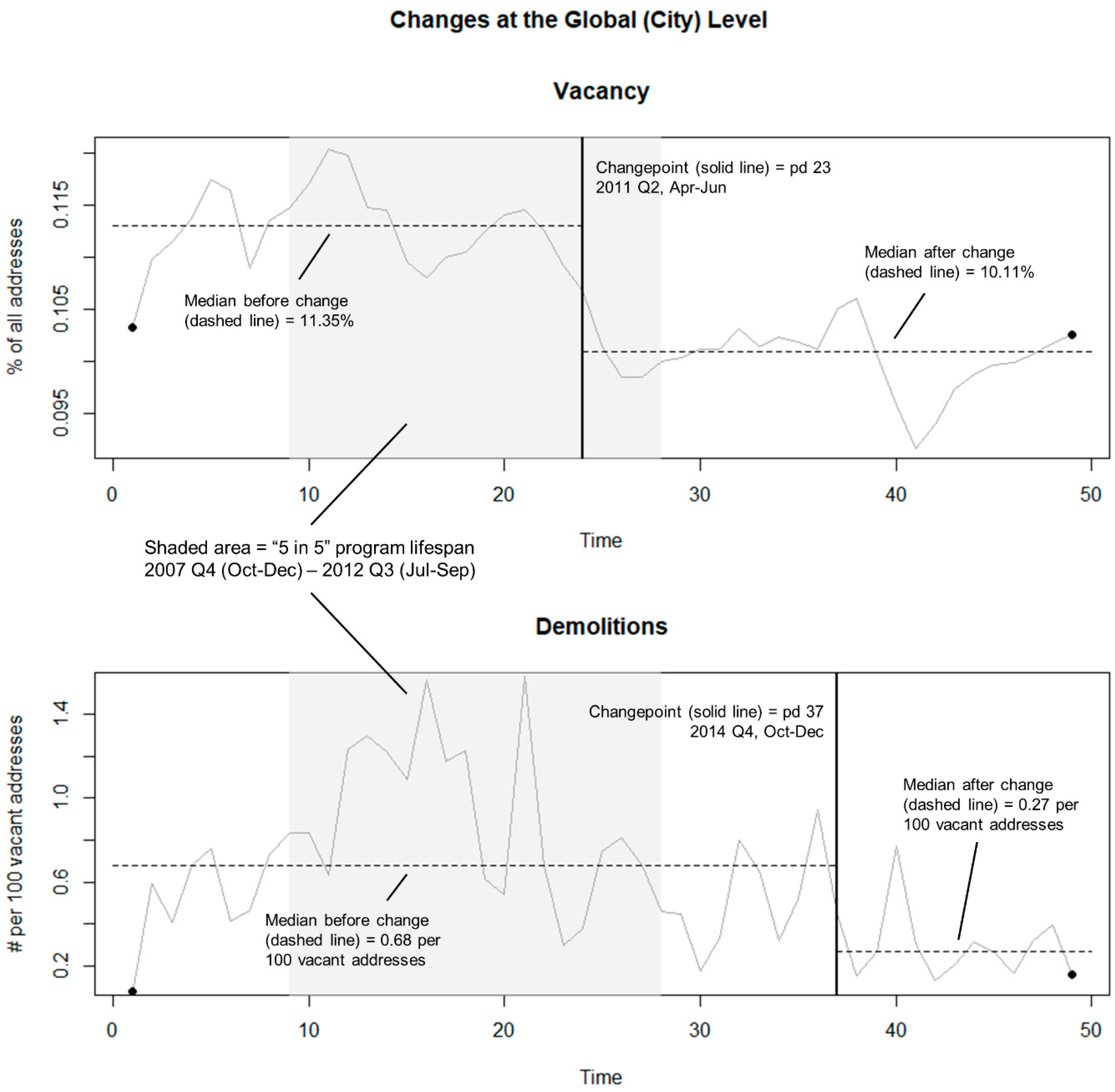
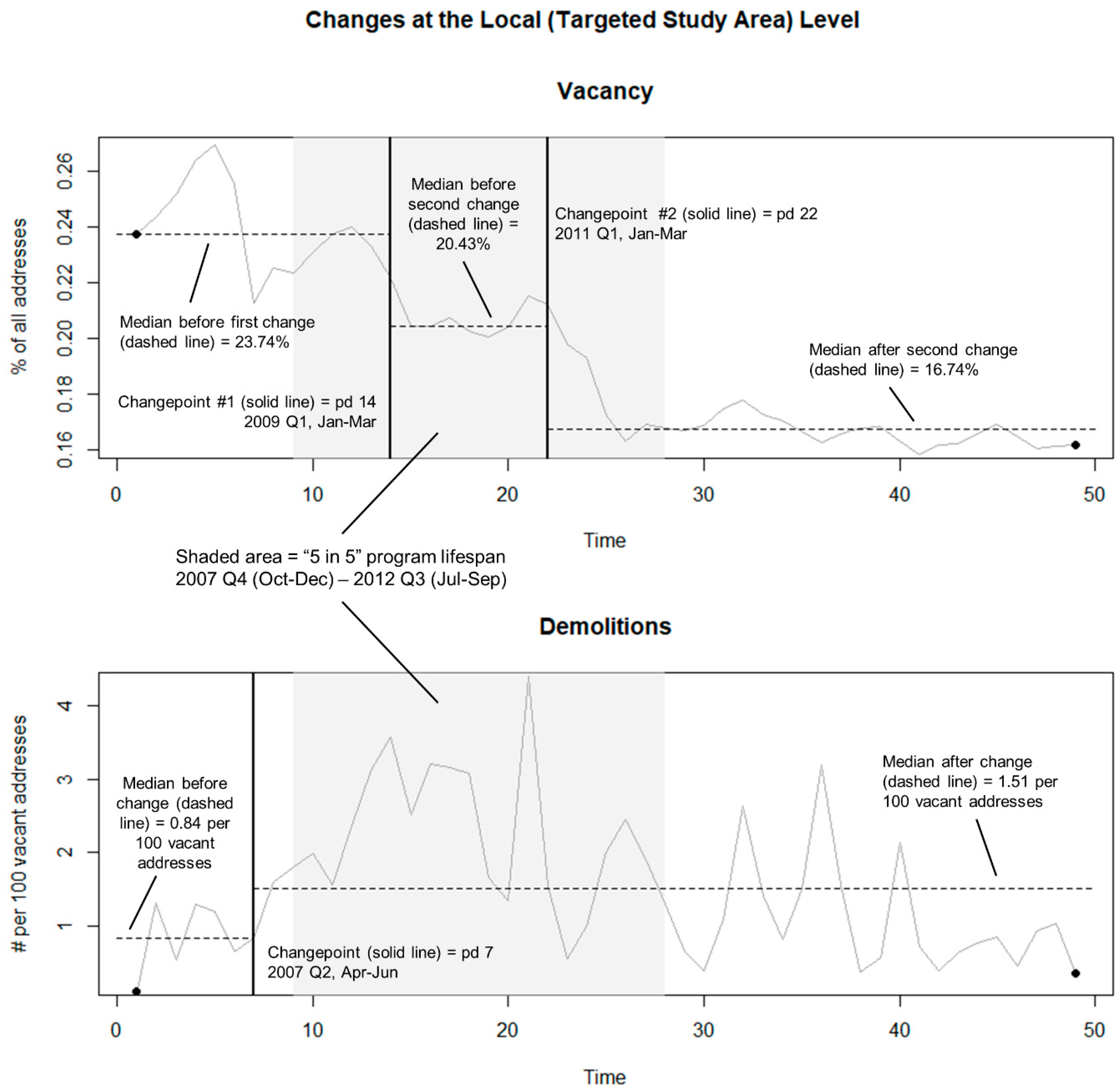
Our second challenge to the notion that aggressive demolition could unilaterally decrease vacancy stocks came in the form of a multi-phase empirical evaluation of the “5 in 5” program conducted in the shrinking city of Buffalo, NY. While other scholars have critiqued this program on the grounds that it was not connected to larger planning frameworks [11,27], it was reactive [33], and that it did not complete its targeted (“aggressive”) number of demolitions [15], we sought to add some empirical weight to this conversation. In particular, we put the foundational assumption—that demolition lowers vacancy—to the test. First, we used spatiotemporal cluster analysis to better understand the spatial footprint of the program. From there, we performed both global (citywide) and local (demolition cluster) changepoint analyses on HUD/USPS vacancy data and city of Buffalo demolition data to establish the optics of the policy. We observed that, in a key administrative dataset used to track vacancy at regular temporal intervals [15], Buffalo appeared to experience a significant drop in vacancy around the time of the “5 in 5” program. While there was no corresponding (statistically significant) uptick in demolition activity despite the aggressive rhetoric of the “5 in 5” program [34], it was still tempting to claim that the city’s seemingly swift response to vacancy (refer to Section 1.3) brought about change. The temptation to reach this conclusion was strongly reinforced when one monitors the same data in the subarea of Buffalo where demolition activity was spatiotemporally clustered. Indeed, in the east-central part of the city, vacancy experienced two significant negative changepoints during the “5 in 5” program, all while demolition experienced a significant increase.
Together, these two sets of results built a strong circumstantial case in favor of Buffalo’s signature demolition program. They also pushed hard against the grain of the systems thinking reasoning described in the preceding paragraph. For that reason, in the final phase of empirical analysis, we directly tested the null hypothesis that the city’s demolition activity caused change in vacancy. Granger-causality tests failed to reject the null hypothesis of no influence, i.e., demolition does 
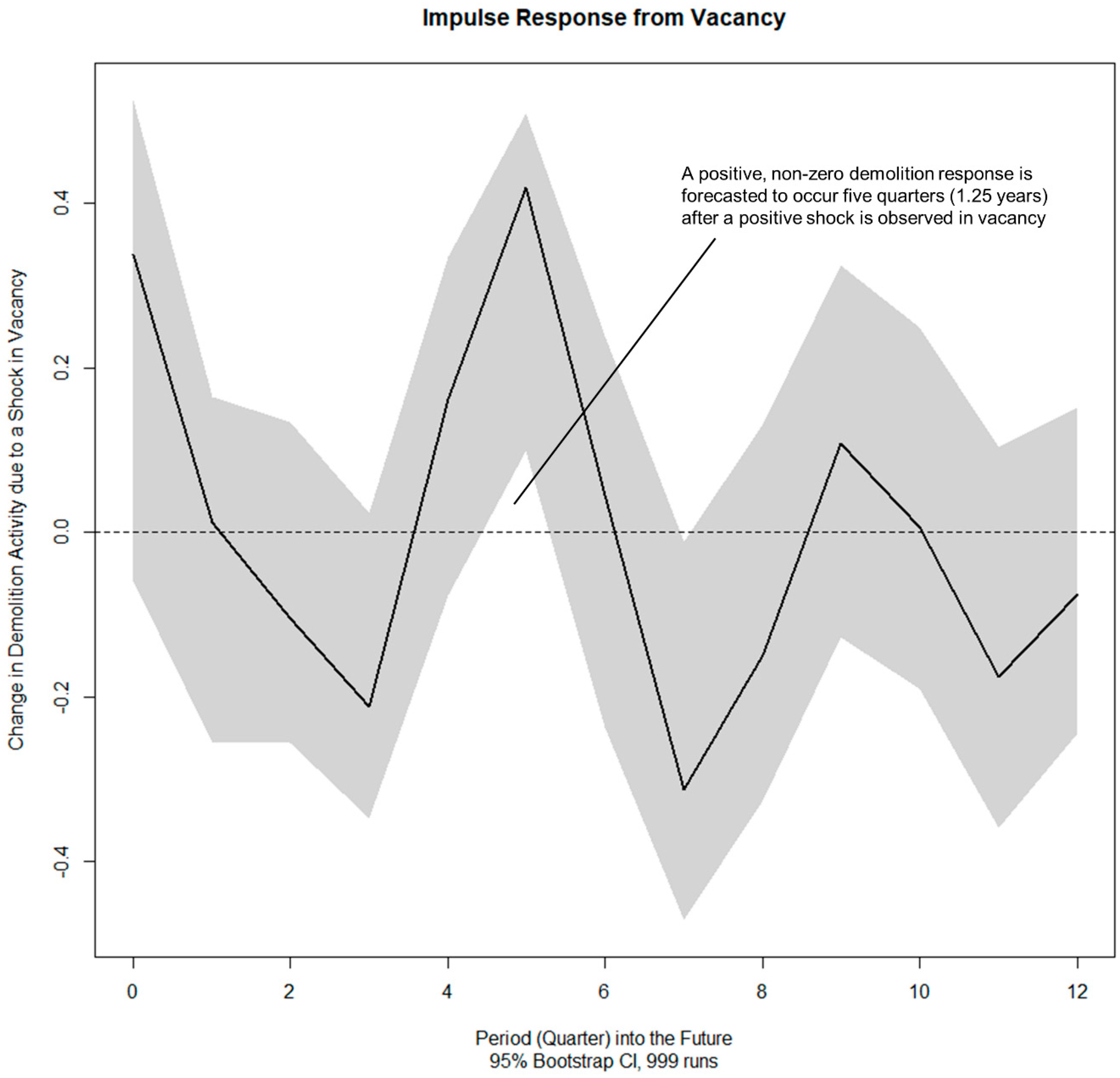
not Granger-cause changes in vacancy stocks, at both the citywide and cluster-wide levels of analysis. At the same time, in the local demolition cluster, we found evidence to support the alternative hypothesis of causality in the opposite direction—that vacancy Granger-causes change in demolition activity. This finding supported speculations that “5 in 5” program was reactive, and, as such, used demolition as a tool in areas perceived to be most affected by vacancy rather than grounding demolition activity in a proactive, comprehensive planning strategy [11,15].
In total, then, the flaw with the “5 in 5” program was not that it was underfunded or that it failed to complete its targeted number (5000) of demolitions. Instead, to the extent that the program was ineffective in its goal of moving the city’s vacancy rate [34], event-oriented thinking atop of a pro-growth mental model were to blame. The city failed to adequately engage with the complexity and dynamics of urban shrinkage and decline (and their many interrelated causes and consequences), preferring to design a “surface-level” solution to a much deeper problem (Figure 1). The hard lesson for shrinking cities is, as many researchers have rightly observed (e.g., [9,11,16,27]), that decision-makers must face the realities of shrinkage and break free from growth-oriented mental models and the toolboxes that those models endorse. Planners and policymakers in shrinking cities will have to embrace context and begin to design innovative instruments aimed at stabilization and improving local quality of life for the residents and buildings who remain “after abandonment” [11,13,22,63].

5. Conclusions

Demolition is a necessary implement in the toolbox of shrinking cities [2,14]. When rolled out in standalone form, however, our study suggests that it is not an effective vacancy management strategy. The built-in demand for developable land that tends to exist in growing cities is generally not part of the structure (Figure 1) of shrinking cities [3]. As such, demolition must be part of broader, comprehensive planning and policy strategies [9,14,35,36,37]. At minimum, complementary efforts are needed (1) to slow or stall the ongoing inflow of property abandonment, and/or (2) to increase the rate at which extant vacant or abandoned properties are reused (Figure 2). In the absence of these efforts, large-scale demolition programs in shrinking cities are destined to remain faith-based vacancy management strategies. Namely, faith is placed in pro-growth mental models (Figure 1) which assume that (1) increasing the supply of vacant land will increase developers’ demand for that land, and (2) the resultant development will create new demand for urban housing. The glaring lack of real world evidence to support these beliefs [3] suggests that decision-makers in shrinking cities must transform their mental models (see Section 1.2.1 and [48]). Strategies built atop these new “right-sizing” [27] or “smart shrinkage” [10] mental models should be informed by dynamic analyses of neighborhood change processes and make use of systems thinking. Seeking to develop better, more systemic understandings of neighborhood dynamics will allow for more proactive and predictive policymaking, as opposed to the reactive trap in which many shrinking cities currently find themselves (e.g., [15]; Figure 7).

Author Contributions

Conceptualization, R.W. and J.K.; Methodology, R.W.; Software, R.W.; Validation, R.W.; Formal Analysis, R.W.; Investigation, R.W. and J.K.; Resources, R.W. and J.K..; Data Curation, R.W.; Writing-Original Draft Preparation, R.W. and J.K.; Writing-Review & Editing, R.W. and J.K.; Visualization, R.W.; Supervision, R.W. and J.K.; Project Administration, R.W. and J.K.

Funding

This research received no external funding.

Acknowledgments

The authors thank the article editor and anonymous peer reviewers for their time and expertise.

Conflicts of Interest

The authors declare no conflict of interest.

Appendix A

Table A1 presents the results of diagnostic tests performed on the AIC-selected VAR candidate models. All tests were carried out with the “vars” R package [60]. Not shown here, OLS-CUSUM tests revealed no issues with (in)stability in any of the three models.
Table A1. Results of Diagnostic Tests for Candidate Models.
Candidate VAR ModelEdgerton-Shukur F-TestMultivariate Jarque-Bera Test for Normality of ResidualsMultivariate ARCH-LM Test for HeteroskedasticityDecision
Null Hypothesis (H0)No serial autocorrelation presentResiduals of VAR are normally distributedNo heteroskedasticity present in VAR--
Global (two lags with a constant and trend)F[20,60] = 1.11
p = 0.37
Do not reject H0
χ 2 [4] = 55.92
p < 0.01
Reject H0
χ 2 [45] = 51.82
p = 0.23
Do not reject H0
Model was selected for analysis due to its superior performance over the remaining candidates; however, note that it does have issues with non-normal errors
Local (six lags with a trend)F[20,38] = 2.65
p < 0.01
Reject H0
χ 2 [4] = 14.32
p < 0.01
Reject H0
χ 2 [45] = 62.75
p = 0.04
Reject H0
Model exhibited numerous problems and was discarded
Local (ten lags with a constant and trend)F[20,12] = 1.41
p = 0.27
Do not reject H0
χ 2 [4] = 5.23
p = 0.26
Do not reject H0
χ 2 [45] = 36.84
p = 0.80
Do not reject H0
Model was selected for analysis

References

  1. Oswalt, P. (Ed.) Shrinking Cities, Volume 2: Interventions; Hatje Cantz Verlag: Ostfildern, Germany, 2006. [Google Scholar]
  2. Mallach, A. Laying the Groundwork for Change: Demolition, Urban Strategy, and Policy Reform; The Brookings Institution: Washington, DC, USA, 2012. [Google Scholar]
  3. Schilling, J.M.; Mallach, A. Cities in Transition: A Guide for Practicing Planners; The American Planning Association Press: Chicago, IL, USA, 2012. [Google Scholar]
  4. Beauregard, R.A. When America Became Suburban; University of Minnesota Press: Minneapolis, MN, USA, 2006. [Google Scholar]
  5. Großmann, K.; Bontje, M.; Haase, A.; Mykhnenko, V. Shrinking cities: Notes for the further research agenda. Cities 2013, 35, 221–225. [Google Scholar] [CrossRef]
  6. Pallagst, K.; Wiechmann, T.; Martinez-Fernandez, C. (Eds.) Shrinking Cities: International Perspectives and Policy Implications; Routledge: New York, NY, USA, 2014. [Google Scholar]
  7. Richardson, H.W.; Nam, C.W. (Eds.) Shrinking Cities: A Global Perspective; Routledge: New York, NY, USA, 2014. [Google Scholar]
  8. Weaver, R.; Bagchi-Sen, S.; Knight, J.; Frazier, A.E. Shrinking Cities: Understanding Urban Decline in the United States; Routledge: New York, NY, USA, 2016. [Google Scholar]
  9. Hollander, J.B.; Pallagst, K.; Schwarz, T.; Popper, F.J. Planning shrinking cities. Prog. Plan. 2009, 72, 223–232. [Google Scholar] [CrossRef]
  10. Hollander, J. A Research Agenda for Shrinking Cities; Edward Elgar Publishing: Cheltenham, UK, 2018. [Google Scholar]
  11. Ryan, B.D. Design After Decline: How America Rebuilds Shrinking Cities; University of Pennsylvania Press: Philadelphia, PA, USA, 2012. [Google Scholar]
  12. Accordino, J.; Johnson, G.T. Addressing the vacant and abandoned property problem. J. Urban Aff. 2000, 22, 301–315. [Google Scholar] [CrossRef]
  13. Weaver, R.C.; Bagchi-Sen, S. Spatial analysis of urban decline: The geography of blight. Appl. Geogr. 2012, 40, 61–70. [Google Scholar] [CrossRef]
  14. Mallach, A. Demolition and Preservation in Shrinking US Industrial Cities. Build. Res. Inf. 2011, 39, 380–394. [Google Scholar] [CrossRef]
  15. Silverman, R.M.; Yin, L.; Patterson, K.L. Municipal property acquisition patterns in a shrinking city: Evidence for the persistence of an urban growth paradigm in Buffalo, NY. Cogent Soc. Sci. 2015, 1, 1012973. [Google Scholar] [CrossRef]
  16. Hospers, G.J. Policy responses to urban shrinkage: From growth thinking to civic engagement. Eur. Plan. Stud. 2014, 22, 1507–1523. [Google Scholar] [CrossRef]
  17. Weaver, R. Palliative planning in an American shrinking city–Some thoughts and preliminary policy analysis. Community Dev. 2017, 48, 436–450. [Google Scholar] [CrossRef]
  18. Weaver, R.; Knight, J. Analysis of a multipronged community development initiative in two distressed neighbourhoods. Commun. Dev. J. 2017, 53, 301–320. [Google Scholar] [CrossRef]
  19. Knight, J.; Weaver, R.; Jones, P. Walkable and resurgent for whom? The uneven geographies of walkability in Buffalo, NY. Appl. Geogr. 2018, 92, 1–11. [Google Scholar] [CrossRef]
  20. Dewar, M.; Kelly, C.; Morrison, H. Planning for Better, Smaller Places after Population Loss: Lessons from Youngstown and Flint. In The City after Abandonment; Dewar, M., Thomas, J.M., Eds.; University of Pennsylvania Press: Philadelphia, PA, USA, 2013; pp. 289–316. [Google Scholar]
  21. Lawson, L.; Miller, A. Community Gardens and Urban Agriculture as Antithesis to Abandonment: Exploring a Citizenship-Land Model. In The City after Abandonment; Dewar, M., Thomas, J.M., Eds.; University of Pennsylvania Press: Philadelphia, PA, USA, 2013; pp. 17–40. [Google Scholar]
  22. Schatz, L. Decline-Oriented Urban Governance in Youngstown, Ohio. In The City after Abandonment; Dewar, M., Thomas, J.M., Eds.; University of Pennsylvania Press: Philadelphia, PA, USA, 2013; pp. 87–103. [Google Scholar]
  23. Leo, C.; Anderson, K. Being realistic about urban growth. J. Urban Aff. 2006, 28, 169–189. [Google Scholar] [CrossRef]
  24. Jessen, J. Conceptualizing Shrinking Cities—A Challenge for Planning Theory. In Parallel Patterns of Shrinking Cities and Urban Growth; Ganser, R., Piro, R., Eds.; Ashgate: Burlington, VT, USA, 2012; pp. 45–58. [Google Scholar]
  25. Roth, H.; Cunningham-Sabot, E. Shrinking Cities in the Growth Paradigm: Towards Standardised Regrowing Strategies? In Parallel Patterns of Shrinking Cities and Urban Growth; Ganser, R., Piro, R., Eds.; Ashgate: Burlington, VT, USA, 2012; pp. 59–72. [Google Scholar]
  26. Schilling, J. Buffalo as the nation’s first living laboratory for reclaiming vacant properties. In Cities Growing Smaller; Kent State Cleveland Urban Design Collaborative: Kent, OH, USA, 2008; pp. 32–44. [Google Scholar]
  27. Schilling, J.; Logan, J. Greening the rust belt: A green infrastructure model for right sizing America’s shrinking cities. J. Am. Plan. Assoc. 2008, 74, 451–466. [Google Scholar] [CrossRef]
  28. Ryan, B.D. Rightsizing Shrinking Cities: The Urban Design Dimension. In The City after Abandonment; Dewar, M., Thomas, J.M., Eds.; University of Pennsylvania Press: Philadelphia, PA, USA, 2013; pp. 268–288. [Google Scholar]
  29. Frazier, A.E.; Bagchi-Sen, S.; Knight, J. The spatio-temporal impacts of demolition land use policy and crime in a shrinking city. Appl. Geogr. 2013, 41, 55–64. [Google Scholar] [CrossRef]
  30. Silverman, R.M.; Yin, L.; Patterson, K.L. Dawn of the dead city: An exploratory analysis of vacant addresses in Buffalo, NY 2008–2010. J. Urban Aff. 2013, 35, 131–152. [Google Scholar] [CrossRef]
  31. Weaver, R.C. Re-framing the urban blight problem with trans-disciplinary insights from ecological economics. Ecol. Econ. 2013, 90, 168–176. [Google Scholar] [CrossRef]
  32. Hummel, D. Right-sizing cities in the United States: Defining its strategies. J. Urban Aff. 2015, 37, 397–409. [Google Scholar] [CrossRef]
  33. Yin, L.; Silverman, R.M. Housing abandonment and demolition: Exploring the use of micro-level and multi-year models. ISPRS Int. J. Geo-Inf. 2015, 4, 1184–1200. [Google Scholar] [CrossRef]
  34. City of Buffalo. Mayor Brown’s “5-in-5” Demolition Plan: Moving Buffalo forward Policy Brief from the Brown Administration; Department of Administration, Finance, and Urban Affairs: Buffalo, NY, USA, 2007.
  35. Johnson, M.P.; Hollander, J.; Hallulli, A. Maintain, demolish, re-purpose: Policy design for vacant land management using decision models. Cities 2014, 40, 151–162. [Google Scholar] [CrossRef]
  36. Hackworth, J. Demolition as urban policy in the American Rust Belt. Environ. Plan. A Econ. Space 2016, 48, 2201–2222. [Google Scholar] [CrossRef]
  37. Morckel, V.C. Empty neighborhoods: Using constructs to predict the probability of housing abandonment. Hous. Policy Debate 2013, 23, 469–496. [Google Scholar] [CrossRef]
  38. Batty, M. Complexity in city systems: Understanding, evolution, and design. In A Planner’s Encounter with Complexity; de Roo, G., Silva, E.A., Eds.; Routledge: New York, NY, USA, 2007; pp. 99–122. [Google Scholar]
  39. Martinez-Fernandez, C.; Audirac, I.; Fol, S.; Cunningham-Sabot, E. Shrinking cities: Urban challenges of globalization. Int. J. Urban Reg. Res. 2012, 36, 213–225. [Google Scholar] [CrossRef] [PubMed]
  40. Beauregard, R.A. Urban population loss in historical perspective: United States, 1820–2000. Environ. Plan. A 2009, 41, 514–528. [Google Scholar] [CrossRef]
  41. United Nations. World Urbanization Prospects: The 2014 Revision; United Nations: New York City, NY, USA, 2014.
  42. Mumford, L. The City in History: Its Origins, Its Transformations, and Its Prospects; Houghton Mifflin Harcourt: Boston, MA, USA, 1961. [Google Scholar]
  43. Weaver, R. Toward a Definitional Framework for Urban Design (1 July 2017), doi:10.2139/ssrn.3009419. Available online: https://ssrn.com/abstract=3009419 (accessed on 1 August 2018).
  44. Downs, A. Neighborhoods and Urban Development; Brookings Institution Press: Washington, DC, USA, 1981. [Google Scholar]
  45. Hollander, J.B. Can a city successfully shrink? Evidence from survey data on neighborhood quality. Urban Aff. Rev. 2011, 47, 129–141. [Google Scholar] [CrossRef]
  46. Meadows, D.H. Thinking in Systems: A Primer; Chelsea green publishing: Burlington, VT, USA, 2008. [Google Scholar]
  47. Nguyen, N.C.; Bosch, O.J.; Maani, K.E. Creating ‘learning laboratories’ for sustainable development in biospheres: A systems thinking approach. Syst. Res. Behav. Sci. 2011, 28, 51–62. [Google Scholar] [CrossRef] [Green Version]
  48. Northwest Institute. A Systems Thinking Model: The Iceberg. Available online: http://www.nwei.org/assets/A-SYSTEMS-THINKING-MODEL-The-Iceberg.pdf (accessed on 1 August 2018).
  49. Bourne, L.S. The Geography of Housing; Halsted Press: Sydney, Australia, 1981. [Google Scholar]
  50. Hjorth, P.; Bagheri, A. Navigating towards sustainable development: A system dynamics approach. Futures 2006, 38, 74–92. [Google Scholar] [CrossRef]
  51. Kantor, P. City futures: Politics, economic crisis, and the American model of urban development. Urban Res. Pract. 2010, 3, 1–11. [Google Scholar] [CrossRef]
  52. ESRI. Create Space Time Cube by Aggregating Points. Available online: http://pro.arcgis.com/en/pro-app/tool-reference/space-time-pattern-mining/create-space-time-cube.htm (accessed on 1 August 2018).
  53. Ross, G.J. Parametric and nonparametric sequential change detection in R: The CPM package. J. Stat. Softw. 2015, 66, 1–20. [Google Scholar] [CrossRef]
  54. Hawkins, D.M.; Zamba, K.D. A change-point model for a shift in variance. J. Qual. Technol. 2005, 37, 21–31. [Google Scholar] [CrossRef]
  55. Ross, G.J.; Adams, N.M.; Tasoulis, D.K.; Hand, D.J. A nonparametric change point model for streaming data. Technometrics 2011, 53, 379–389. [Google Scholar] [CrossRef]
  56. Ross, G.J. Package ‘CPM’. CRAN Network. 2015. Available online: https://cran.r-project.org/web/packages/cpm/cpm.pdf (accessed on 1 August 2018).
  57. Granger, C.W. Investigating causal relations by econometric models and cross-spectral methods. Econometrica 1969, 37, 424–438. [Google Scholar] [CrossRef]
  58. Pfaff, B. Analysis of Integrated and Cointegrated Time Series with R, 2nd ed.; Springer: New York, NY, USA, 2008. [Google Scholar]
  59. Sorensen, B.E. Granger Causality. Available online: http://www.uh.edu/~bsorense/gra_caus.pdf (accessed on 1 August 2018).
  60. Pfaff, B.; Stigler, M. Package ‘VARS’. CRAN Network. 2015. Available online: https://cran.r-project.org/web/packages/vars/vars.pdf (accessed on 1 August 2018).
  61. ESRI. How Emerging Hot Spot Analysis Works. Available online: http://pro.arcgis.com/en/pro-app/tool-reference/space-time-pattern-mining/learnmoreemerging.htm (accessed on 1 August 2018).
  62. Hafner, C.M.; Herwartz, H. Testing for linear vector autoregressive dynamics under multivariate generalized autoregressive heteroskedasticity. Stat. Neerl. 2009, 63, 294–323. [Google Scholar] [CrossRef]
  63. Dewar, M.; Thomas, J.M. (Eds.) The City after Abandonment; University of Pennsylvania Press: Philadelphia, PA, USA, 2013. [Google Scholar]
Figure 1. The iceberg model of systems thinking.
Urbansci 02 00069 g001
Figure 2. A basic stock and flow diagram of vacancy and abandonment in a shrinking city.
Urbansci 02 00069 g002
Figure 3. Change in vacant addresses as a fraction of total mailing addresses (top) and demolished structures per 100 vacant addresses (bottom) in Buffalo, NY from October 2005 through December 2017. Each time step represents a quarter. Time-step 1 is Q4 of 2005, and the ending time-step 49 is Q4 of 2017. The shaded areas represent the time horizon of the “5 in 5” demolition program.
Urbansci 02 00069 g003
Figure 4. The distribution of all public demolitions completed from 5 October 2005 through to December 20, 2017 (on left), and the results of the space-time cluster analysis of that distribution (on right). Observe that the pattern of “5 in 5” demolitions mirrors demolition activity before and after the program was implemented. In other words, the geography of demolitions during “5 in 5” was not substantially different from time periods before and after the program. What was perhaps different was the magnitude. On the right panel, observe that sporadic, consecutive, and persistent hotspots of demolitions occurred in the eastern portion of the city. The highlighted area is the set of all U.S. census tracts intersected by these various types of hotspots.
Urbansci 02 00069 g004
Figure 5. Changepoints detected in citywide vacancy (top) and demolition (bottom) between Q4 2005 (period 1) and Q4 2017 (period 49).
Urbansci 02 00069 g005
Figure 6. Changepoints detected in vacancy (top) and demolition (bottom) between Q4 2005 (period 1) and Q4 2017 (period 49) for the “Local Study Area” depicted in Figure 4.
Urbansci 02 00069 g006
Figure 7. Impulse response of demolition activity to a one standard deviation (positive) shock in vacancy. Significantly higher demolition is estimated to happen five quarters after the shock.
Urbansci 02 00069 g007
Table 1. Definitions of Cluster Types Identified in Figure 4.
Cluster TypeDefinition 1
Consecutive Hotspot“A location with a single uninterrupted run of statistically significant hot spot bins in the final time-step intervals. The location has never been a statistically significant hot spot prior to the final hot spot run and less than ninety percent of all bins are statistically significant hot spots.”
Persistent Hotspot“A location that has been a statistically significant hot spot for ninety percent of the time-step intervals with no discernible trend indicating an increase or decrease in the intensity of clustering over time.”
Diminishing Hotspot“A location that has been a statistically significant hot spot for ninety percent of the time-step intervals, including the final time step. In addition, the intensity of clustering in each time step is decreasing overall and that decrease is statistically significant.”
Sporadic Hotspot“A location that is an on-again then off-again hot spot. Less than ninety percent of the time-step intervals have been statistically significant hot spots and none of the time-step intervals have been statistically significant cold spots.”
New Cold Spot“A location that is a statistically significant cold spot for the final time step and has never been a statistically significant cold spot before.”
Consecutive Cold Spot“A location with a single uninterrupted run of statistically significant cold spot bins in the final time-step intervals. The location has never been a statistically significant cold spot prior to the final cold spot run and less than ninety percent of all bins are statistically significant cold spots.”
Intensifying Cold Spot“A location that has been a statistically significant cold spot for ninety percent of the time-step intervals, including the final time step. In addition, the intensity of clustering of low counts in each time step is increasing overall and that increase is statistically significant.”
Persistent Cold Spot“A location that has been a statistically significant cold spot for ninety percent of the time-step intervals with no discernible trend, indicating an increase or decrease in the intensity of clustering of counts over time.”
Sporadic Cold Spot“A location that is an on-again then off-again cold spot. Less than ninety percent of the time-step intervals have been statistically significant cold spots and none of the time-step intervals have been statistically significant hot spots.”
Oscillating Cold Spot“A statistically significant cold spot for the final time-step interval that has a history of also being a statistically significant hot spot during a prior time step. Less than ninety percent of the time-step intervals have been statistically significant cold spots.”
No Pattern DetectedDoes not fall into any of the hot or cold spot patterns defined above.
1 Descriptions come from Reference [61].
Table 2. Granger test results of the null hypothesis: demolition does not cause change in vacancy.
Study AreaNumber of Boot Runsp-ValueDecision
Global: City of Buffalo9990.6266Do Not Reject: Demolition does not Granger-cause change in vacancy
Local: Demolition Cluster9990.2282Do Not Reject: Demolition does not Granger-cause change in vacancy
Table 3. Granger test results of the null hypothesis: vacancy does not cause change in demolition.
Study AreaNumber of Boot Runsp-ValueDecision
Global: City of Buffalo9990.1011Do Not Reject: Vacancy does not Granger-cause change in demolition
Local: Demolition Cluster9990.0250Reject at a 95% Confidence Level: Vacancy Granger-causes change in demolition

