Urban Commute Travel Distances in Tehran, Istanbul, and Cairo: Weighted Least Square Models

Abstract

A very large part of the literature on urban commute travels is related to high-income countries. The determinants of urban commute trip distances are not clear in the Middle East and North Africa (MENA); thus, this study attempts to shed light on this topic in relation to Tehran, Istanbul, and Cairo. The objective is to clarify which environmental and human factors are correlated with commuting distance in these cities. Using primary disaggregate data produced by surveys in the three cities (n = 8237) in 2017, weighted least square regressions showed that fifteen significant or highly significant variables, including individual and household characteristics, mobility decisions, residential location, and land use attributes, predict the lengths of urban commute trips in the MENA sample. Unlike western countries, age and gender are not significant predictors of commute distance in MENA large cities. The results of independent-sample Kruskal–Wallis test show that there is a significant difference between the mean one-way commute travel distances in the three cities (Tehran: 9096 m, Istanbul: 10839 m, and Cairo: 6670 m); however, there are some similarities in the determinants of commute distance in the three cities. The results can be adopted to reduce commute trip lengths by providing a more connected street network and accessible neighborhood-level facilities.

1. Introduction

As one of the main aspects of urban travel, commuting travel time is directly related to commuting distance [1,2,3]. Travel distance, in general, can be an indicator of travel cost [4]. As a factor highly associated with travel length, travel time is a strong predictor of mode choice [5]. Reducing commuting distance—and, as a result, time—may increase individual satisfaction regarding commuting [6]. Long travel distances to work can have unwanted societal and individual consequences, e.g., long commutes by different modes can cause individual stress as a result of long durations of exposure to environmental stressors [7,8,9]. Recent studies have explored the details of individual life circumstances in relation to the costs of long-distance commuting, e.g., couples who commute long distances daily are at greater risk of separation [10]. Thus, shortening commuting lengths in urban areas can be a major mobility-related mission of decision makers.

Hence, understanding the determinants and circumstances of urban commute travel is important for policymakers. However, the insights offered by the international academic literature may not be adopted for planning in all contexts. These publications primarily come from high-income countries, with the conditions and cultural background of those areas. In many planning and research efforts in emerging countries, western studies are perceived as trustable sources of knowledge and the effects of culture, geography, climate, etc., in local contexts are forgotten. Like many other aspects of transportation and travel behavior, commuting distance may be affected by these local phenomena and conditions. Our understanding of the role of contextuality in urban transportation behaviors, intentions, and decisions is very limited. Thus, this manuscript can help to present topically similar research results which then can be used as the basis for contextual comparisons of urban travel behaviors. From a broader perspective, this paper is not only useful to examine commute travel distances but also helps international researchers understand the context-specific nature of commute trips and travel behaviors and decisions in general. This will help us understand that urban planning and urban transport policymaking should be done in accordance with local behaviors and contextual specifications. Therefore, this paper aims to draw the attention of scholars not only from the Middle East and North Africa (MENA) region but from all other regions of the world. Apart from the international importance of the issue of contextuality of transport behaviors, this contribution can be important for policymaking inside the MENA region. Considering the region’s vast area, large population, and high urbanization rate, it will be an internationally important transportation issue that deserves the attention of a large audience from several countries.

The scientific contribution of this paper is novel and original because of, firstly, the novelty of the research within the region and, secondly, the techniques applied to quantify the urban form and commuting distance in the international context. An international team collected the data in the three case-study cities and quantified the commute distances by asking interviewees about their living areas and workplaces. More importantly, the commute distances have been calculated in a disaggregate manner based on the street network. The difficulty of this method has stopped several studies from providing more precise results. Finally, the sample size is large enough to enable statistical power. These research characteristics in a less-studied region provide a desirable level of originality and novelty. This may be continued in future studies on the region.

The objective of this study is to provide a basic understanding about the characteristics of commute distance in three large agglomerations of the MENA region, namely Tehran, Istanbul, and Cairo. In the absence of high-quality disaggregate data, the travel behaviors in this region have been studied less than necessary and policies have been made based on international transportation planning norms that are founded on western studies. In this study, MENA refers to the Middle East, North Africa, Turkey, Mauritania, Sudan, and Somalia.

As mentioned above, one of the emphases of this paper is the contextual differences of commute trips in an international context. Although there are several studies on the topic of urban commute distances, the number of empirically oriented studies that focus on the determinants of urban commuting distances are not considerable. Methodological dissimilarities, such as lack of identical variables, sample sizes, etc., have made comparative studies difficult. The comparisons presented in the discussion section of this paper are established by the findings of this study and a limited number of methodologically similar studies in western countries.

This paper continues with a short review of international studies that provide empirical findings in the form of statistical models, with dependent variables of commuting distance or time. The intention of this section is to integrate the correlation of different factors with the distance of work trips in different contexts. Then, the methodology, including the three research questions and hypotheses of this study, is explained. The findings of a weighted least squares model for the overall sample, consisting of the three cities and models for each of the cities as well as some insights into the distribution and values of commute distances in the case-cities, are described in the findings section. These findings show which environmental and human factors are correlated with commuting distance. Finally, the contextual differences of the determinants of commuting length in the three cities with those of high-income or western countries are sought and some implications related to the built environment are addressed.

2. Determinants of Urban Commute Travel Distances

Urban commute distances have already been examined in the context of the global west, including North American and western countries [11,12,13]. The share of other contexts such as emerging and developing countries of even Eastern Asia is very small. As seen in this short review, a very large part of the literature is based on the USA, Canada, and the Netherlands. This sample of studies on the determinants of commuting length has only one study out of the context of North America and Western Europe, which was conducted on Seoul, South Korea. Since travel distances are highly associated with network-based travel distances, by as much as 80 percent according to Rietveld, Zwart, van Wee, and van den Hoorn [14], and in fact they have appeared together in the same publications, some of the studies related to work trip times have also been summarized in this short review. In Montreal, gender is a determinant of commuting distance: women travel longer distances to access workplaces in the central business district compared to men. However, women’s overall commutes are shorter than those of men [15].

One of the older studies of this type was conducted by Gordon et al. [16], who used the 1980 data of 19 urbanized areas in the United States with population densities greater than 3500 persons per square mile and for the 20 largest urbanized areas. Their linear regression showed that polycentric and dispersed metropolitan areas facilitate shorter commuting times and there is a positive correlation between commuting time and commercial density. Miller and Ibrahim [17] carried out linear regression on the 1986 data of the Transportation Tomorrow Survey relating to six regional municipalities of Toronto, Durham, York, Peel, Halton, and Hamilton-Wentworth in the Greater Toronto Area, Canada, and concluded that living near the cites’ cores or other high-density employment centers is correlated with work trip vehicle kilometers traveled. They also noted that job-housing balance and population density are weak predictors or have no correlation at all: “VKT (Vehicle Kilometers Traveled) per worker increases as one moves away from both the central core of the city and from other high-density employment centers within the region; job-housing balance, per se, shows little impact on commuting VKT; and population density, in and of itself, does not explain variations on commuting VKT once other urban structure variables have been accounted for.” In the Netherlands, the results of a linear regression analysis showed that personal attributes such as education, gender, and age are strong predictors of commute trip distance. Household car ownership is a predictor of length of work travel by car, biking, and walking but not by public transit. Household income is only related to commute trips by car. This study was undertaken using the Dutch National Travel Survey data of 1998 [18].

As one of the few works that did not apply linear regression, the results indicated that “presence of children, occupation of the male worker, and the relative order of the last residential change and the last change in the female worker’s workplace are important determinants of female and male commuting time parameters in household residential location utility functions”. They applied multinomial logistic regression to the data of San Francisco Bay Metropolitan Area. A multiple linear regression of the data of 73,566 individual commuters who resided in the city of Seoul, South Korea in 1995, showed that gender, full-time work, and education are related to commute distance [19]. The results of a simple linear regression on the 1991 Northern Ireland Census of Population concluded that employment, owning no car within the household, degree of deprivation using the Robson Index of Multiple Deprivation, and percentage of families who are Catholic (religion) are correlated with work trip distance [20]. A piece of work representing Scandinavian results showed that “telework reduced by 0.7% the total kilometres travelled in Finland. The probability of working from home increases with commuting distance, but when the commuting trip exceeds 100 km a second apartment near the workplace becomes common and has a stronger impact on commuting kilometres travelled than telework.” This work was done by binary logistic regression on a sample of 838 teleworkers obtained from aggregate national data of 19,000 employed respondents in Finland in 2001 [21].

In addition to Schwanen et al., the Dutch contributions to this topic have yet generated more results. Most of these works especially examine urban form traits, e.g., Ettema et al. conducted binary logistic regression on a sample of 707 diary-days of couples from 2033 households who filled out a 2-day travel/activity diary in the Amsterdam–Utrecht region relating to the year 2000. They noted that commuting time is positively correlated with working for females and out-of-home personal business including education and social visits is negatively related to commute distance in males [22]. In Canada, Mercado & Páez (2009) worked on the data of the Transportation Tomorrow Survey of Hamilton (1996), including 16,190 individuals with a corresponding total of 50,860 trips. The results of their multiple linear regression confirmed that age, gender, employment constraints, household contextual factors, and commercial and residential mix are correlated with commute travel distance. The study that was conducted on the city of Hamilton, near Toronto, Canada, asserts especially that the demographic aging factors have importance in determining commuting distance. The results also showed that high commercial and residential mix has a negative relationship with commute length only in the case of car-based travel [23]. In 2010, Manaugh and colleagues [24] applied linear regression to the 2003 destination survey of over 30,000 home-to-work automobile trips in the Montréal metropolitan region (2003) and concluded that the number of vehicles, male gender, age, low income, full-time employment, number of daily trips, and traveling to a destination in a mixed-use area are among the variables that are correlated with commute distance. Finally, the multivariate models of Antipova et al. [25] on a sample of 1104 working individuals obtained from the 1997 Baton Rouge Personal Transportation Survey (USA) showed that jobs to workers ratio, part-time job, and secondary disadvantage factors such as part-time and immigrant workers with young dependents have a negative correlation with commute distance. Additionally, a study on Flanders, Belgium examined some of the urban traits such as density, diversity, minimum commuting distance, jobs–housing balance, and job accessibility and concluded that a compact city model can be useful for controlling commute length [26].

A methodological issue seen in these publications is that census data are the main source of examining commute distance. The reason behind the lack of support by primary data lies in the difficulty of producing primary data on commute distances. Since census and transportation surveys lack many land use and lifestyle attributes, models developed out of secondary data more or less lack some of the important variables needed to explain variances in commute length. Some of the factors that deserve more investigation are related to the built environment. Among these qualities, the usual land use elements such as land use mix or density have drawn more attention. However, there are several other qualities that may be analyzed in models more frequently. These include access to local facilities and street network characteristics such as connectivity. Due to the difficulty of generating such variables, they have seldom found a place in commute distance models. It should also be mentioned that recent studies have focused on push measures like socio-economics and measures that function as obligations in defining commute distance. Workers usually find a workplace and then commute from their pre-existing living place, so the built environment has a less strong direct push effect. Thus, these factors have been included in models less often. Nevertheless, the built environment variables may be important in relation to non-work activities. The logic is that, if a large share of non-work activities such as daily shopping or social activities can be done in the vicinity of the living place, then the trip chain to work might become shorter. Thus, this shortcoming in the recent literature has gained attention in the present study.

It will be helpful for further development of our understanding about the holistic travel behaviors and decisions, regardless of the geographical and cultural context, to emphasize the following research specifications: (1) to focus on lesser known contexts, so that a balance among the world regions is developed. The majority of studies on commute length have been done on high-income or western contexts. Two exceptions are studies conducted on Tel Aviv and Beijing [27,28]; (2) to apply primary data collected according to research needs and designed particularly to answer the study necessities in contrast to the restrictions of difficulties of using census data. Most of the comparable studies on commute distance are based on census data [20,24,29,30,31,32,33]; (3) production of disaggregate data which facilitate generation of land use and urban form variables; (4) strengthening the balance of variables in favor of the built environment factors by development of disaggregate urban form variables for each subject. This short literature review applied the most similar studies to the present research result in terms of methodology and model generation. However, almost all of the reviewed studies do not employ all of the above data and context specifications. The lack of such a concentration will lead to either inappropriateness and inconsistency of overall research interpretation and/or lack of analysis and modeling power. This study has brought the above four aspects of data collection and case study under one umbrella. In most cases, the studies undertaken in high-income countries do not examine all of these characteristics at the same time.

3. Methodology

3.1. Research Questions and Hypotheses

This research was formulated to answer three research questions: (1) What are the determinants of urban commute travel in Tehran, Istanbul, and Cairo? (Since the culture and religion, geography and climate, infrastructure, and several other factors are similar in these cities, it makes sense to analyze the city-level samples in one overall sample and analyze them together. Moreover, the studies and findings of these three cities together are generalizable and transferable to 27 large cities of more than one million inhabitants in the region [34]); (2) Are the commuting distances different in these three cities?; (3) What are the differences between the characteristics of urban commute travel in these three cities? For the purpose of this study, it is hypothesized that different socio-economic, land use, self-selection, and mobility habit-related variables determine the lengths of urban commute trips in the megacities of the MENA region. These determinants are slightly different in Tehran, Istanbul, and Cairo, but there is overall similarity between the determinants and their power.

3.2. Data

The current study was conducted using a dataset concluded from a survey of 18 neighborhoods of different urban form types including traditional, in-between, and new developments in Tehran, Istanbul, and Cairo carried out in the first half of 2017. The above three eras were initiated slightly differently due to political, socio-economic, and urban planning-related phenomena in the three countries. The neighborhood selection was done in a way that 2 neighborhoods of each era were taken in each city using the following eras: Tehran: before 1930, 1930–1980, and after 1980; Istanbul: before 1950, 1950–1980, and after 1980; Cairo: before 1869, 1869–1975, and after 1975 (traditional, in-between, and new development, respectively). The dates refer to the periods when the neighborhoods were developed or virtually took their final form. According to this typology, “traditional urban form” is defined as a sort of neighborhood that is seen in the historical cores of cities or old rural areas subjected to urban growth. Many of these neighborhoods have a discernible neighborhood center (particularly in Cairo and Tehran) and are fairly compact. The buildings of such neighborhoods are attached to one another and no leapfrog developments are seen within the texture of this typical neighborhood. The second type of urban form, “in-between”, consists of semi-grid street networks with lower population and/or construction compactness compared to traditional neighborhoods. Finally, the third urban form type, “new development”, includes centerless neighborhoods, the majority of which have full-grid street networks.

The data collection was undertaken using direct questioning (face-to-face interviews). Responders were interviewed on the streets of the selected case-study neighborhoods. We attempted to interview the residents of case neighborhoods randomly, but at the same time, interviewers tried to talk to people of diverse ages and genders. Prior to the main survey, a pilot survey of 200 interviews was conducted in five neighborhoods of the three cities to make the questions and options more precise. After the main survey, 8284 validated subjects (Tehran: 2717, Istanbul: 2781, and Cairo: 2786) were acquired after validation and data cleaning. The average age of the respondents was 35.2 years in Cairo, 35.9 in Istanbul, and 38.1 in Tehran. The car ownership rate in the Istanbul sample was lower than in the Tehran and Cairo samples (0.7, 1, and 1.2, respectively). The number of driving licenses per household in Tehran (≈2.5) was considerably higher than in the other two cities. Basically, 24 continuous and 23 categorical variables were generated at the first step according to the raw data of the questionnaire and the land use quantifications. The 24 developed continuous variables were age, household car ownership, no. of driving licenses in household, household income, monthly living cost, frequency of commute trips, no. of non-work activities, last relocation time, commuting distance (m), intersection density (nodes/ha), link-node ratio, street length density (m/ha), no. of accessed facilities, no. of accessed bakeries, no. of accessed clinics, no. of accessed mosques, no. of accessed parks, no. of accessed schools, access to bakeries (m), access to mosques (m), access to clinics (m), access to schools (m), access to parks (m), and access to facilities (m). The 23 categorical variables were gender, activity, individual driving license ownership, commute mode choice, reason for car use, shopping-entertainment place inside the neighborhood, attractive shopping centers in neighborhood, frequency of public transit trips, subjective security of public transport, residential location choice, shopping-entertainment mode choice outside neighborhood, reason for not cycling, entertainment place, reason for no social activity in neighborhood, reason for public transit use, reason for no public transit use, reason for not walking, shopping-entertainment mode choice outside neighborhood, shopping-entertainment mode choice in neighborhood, shopping-entertainment mode choice in neighborhood, sense of belonging to neighborhood, cycling, and neighborhood attractiveness perception.

The final overall sample included between 420 and 476 subjects for each neighborhood. The number of subjects in each neighborhood sub-sample consisted of between 5.1% and 5.7% of the overall sample. The number of interviews in each neighborhood sub-sample made up 0.39% (Basaksehir and Basak in Istanbul) to 2.59% (Golestan-Sharghi in Tehran) of the actual inhabitants of the neighborhood. However, for the household variables, the actual proportion of respondents of each neighborhood is around four times higher dependent on the household size of the related city. The neighborhood-level confidence intervals of the findings were 4.5% to 4.7% for individual variables and 1.8% to 2.4% for household variables. In summary, all of the sample sizes of the neighborhoods are representative considering the inhabitants of all age groups living in them, with a confidence level of less than 5%. The overall sample is representative of the population of all ages of the three cities, with a confidence level of 1.08%, though this representativeness at this level remains theoretical and only the neighborhood-level representativeness should be relied on in this study. The full details of the survey were already published [35].

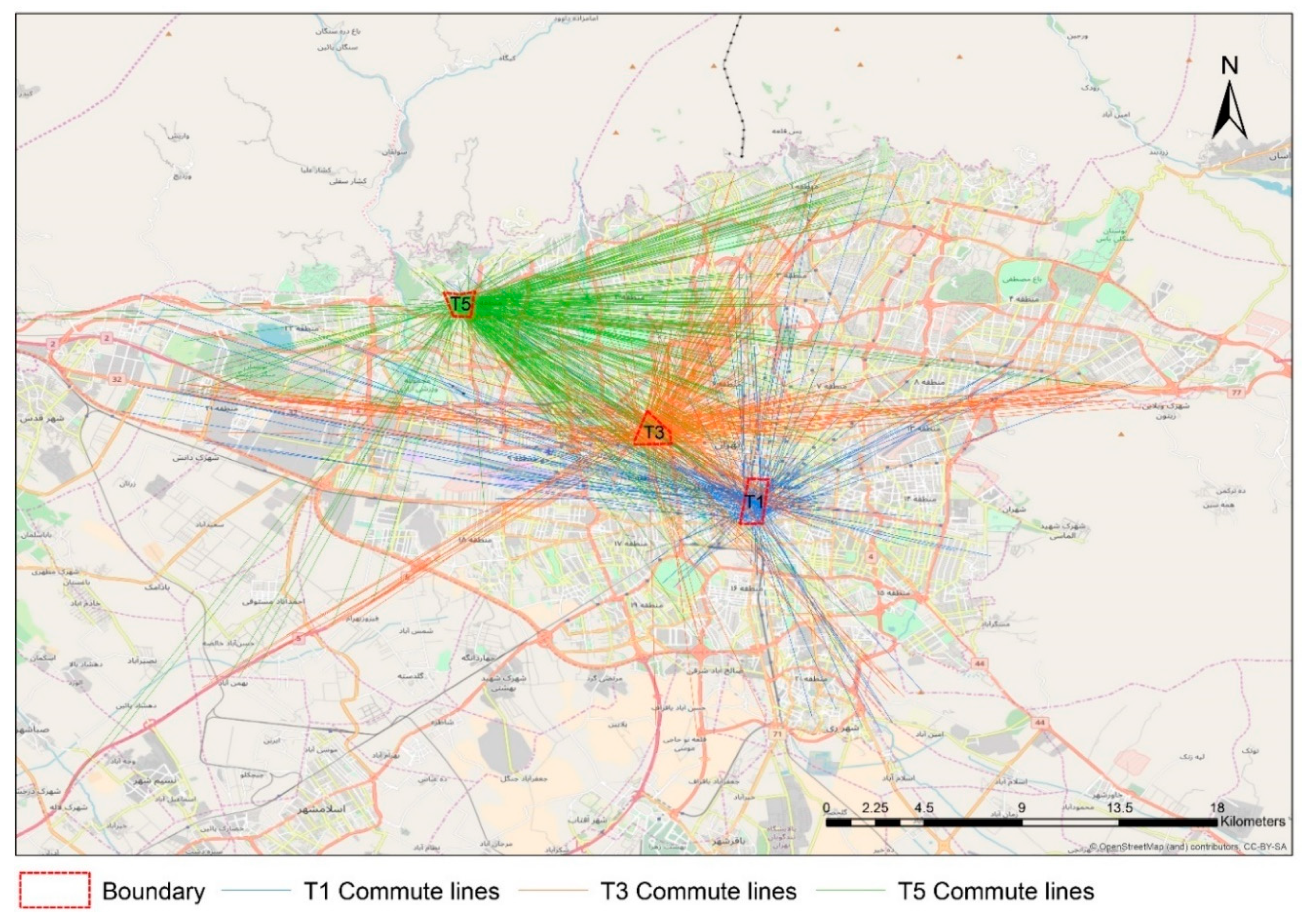
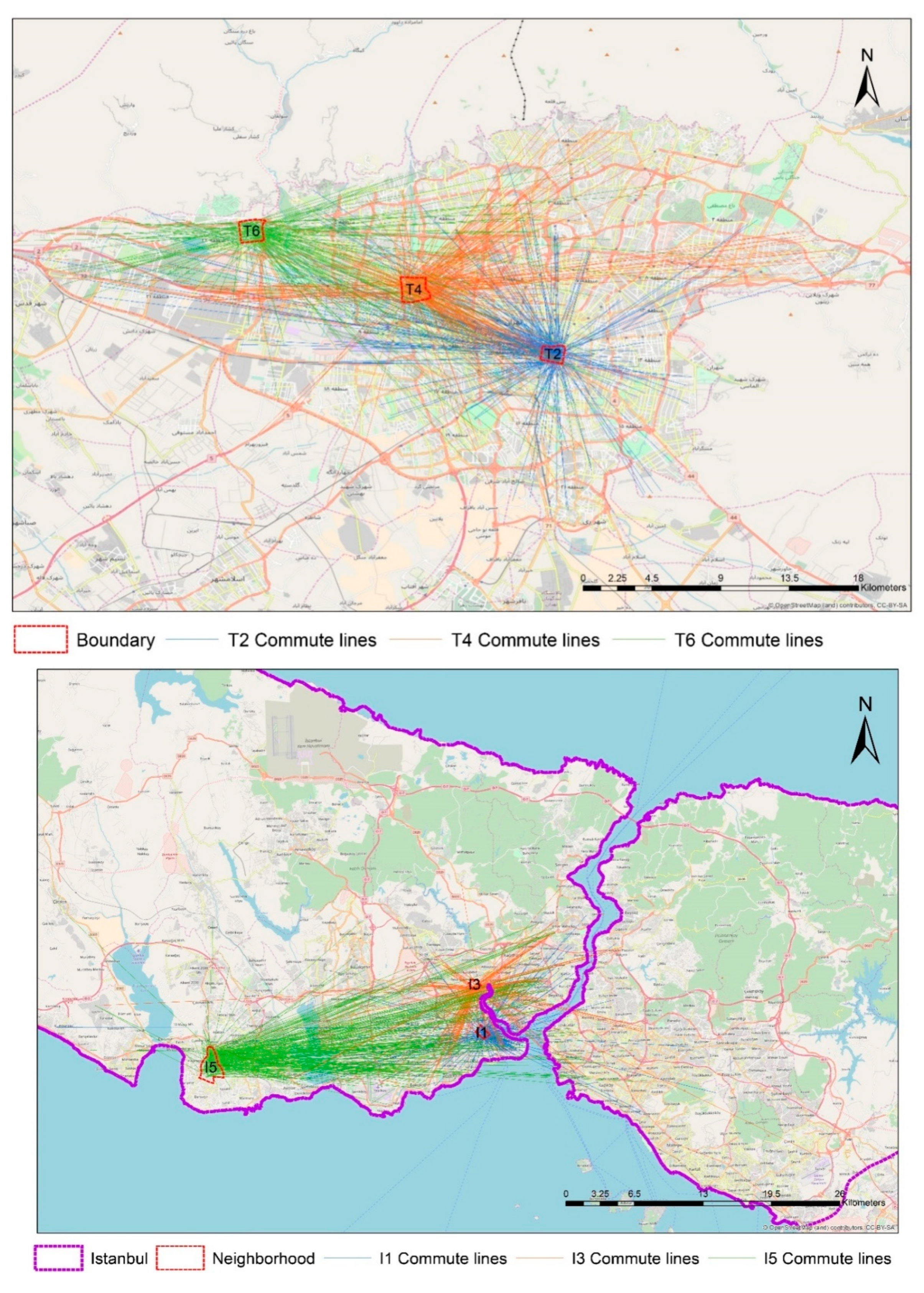
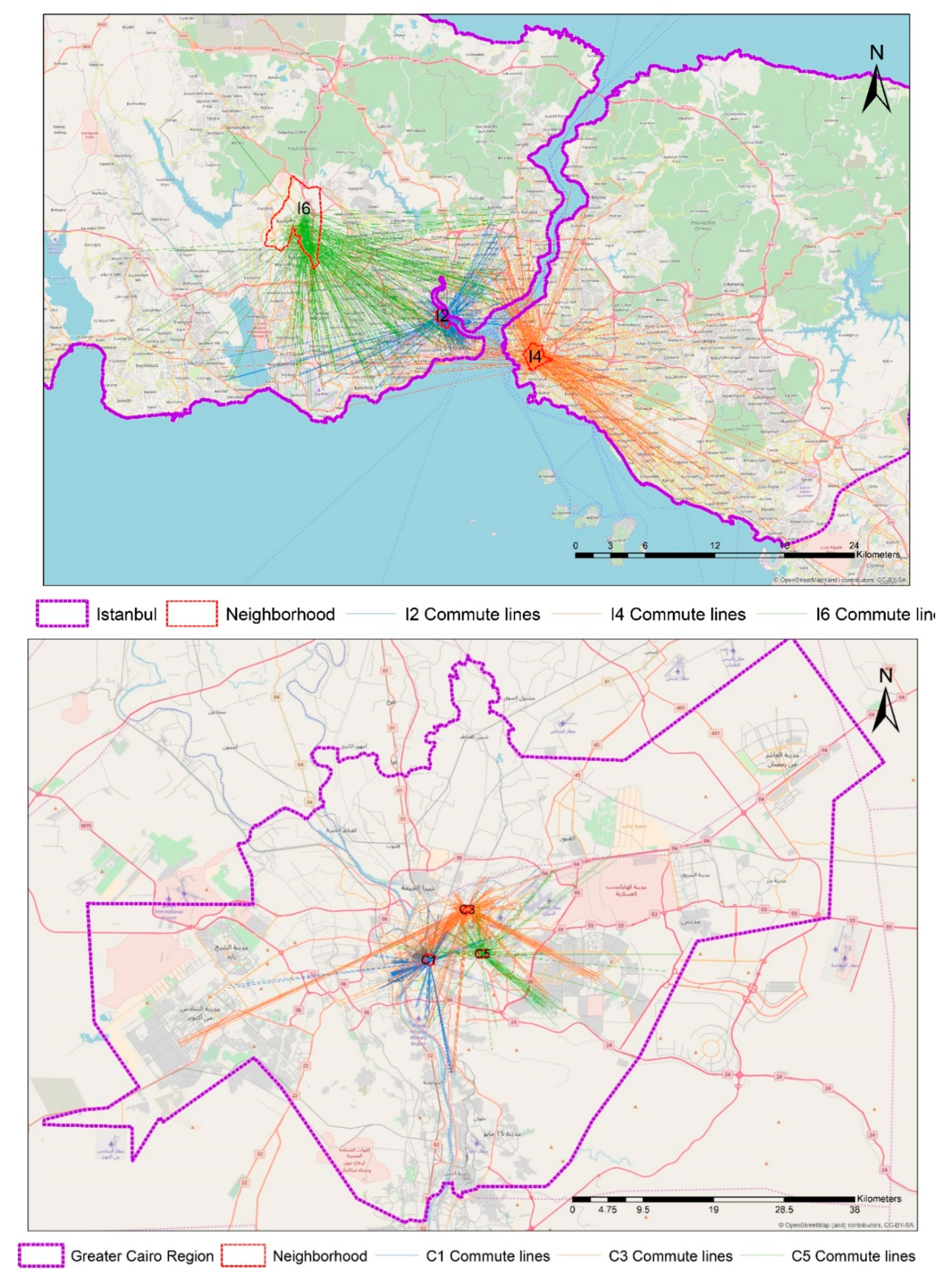
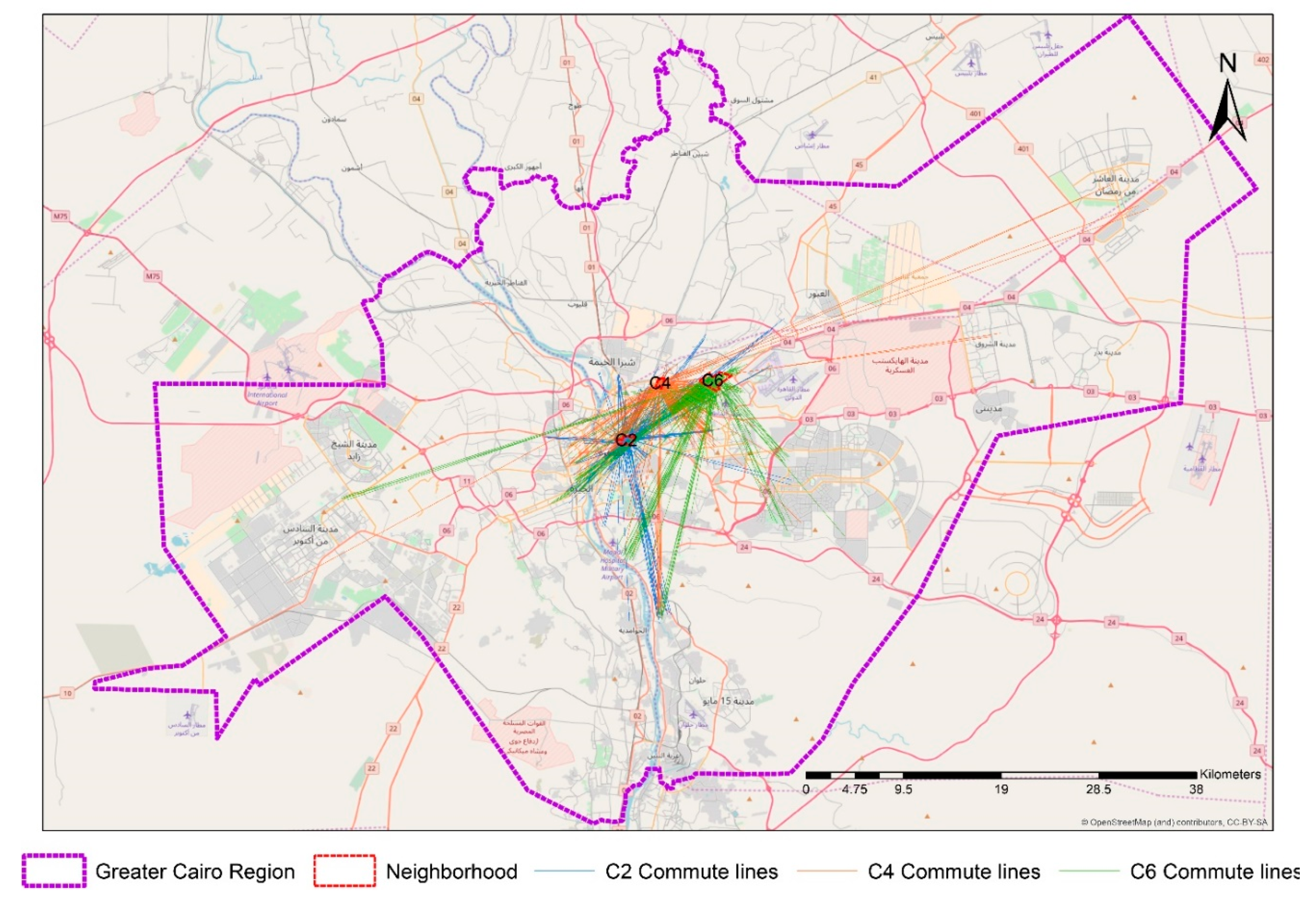
In order to measure the commute distances of the respondents, information about the nearest intersection or landmark to their living and working places were collected at the end of the interviews. This was carried out in order to ensure the participants’ privacy. The two last questions of the survey instrument that were meant to collect this information were “please sign the place of the nearest intersection of streets to your house on Map 1 (attached)” and “if you work or study, please sign the place of the nearest intersection of streets to your working place on Map 2 (attached)”. Since the second question was conditional, 62.2% of the respondents answered this question. The interviewers signed the places on the neighborhood and city maps. Then, the survey office staff estimated the commuting distances based on street networks by means of ArcGIS software. In this method of calculating commute length, the most important factor is the objective value of distance, while other issues like speed, preferences, or modes are assumed to be ineffective. The reason is that such issues are included in the model in other variables; hence, including them in commute distance would cause multicollinearity. The output lengths produced a disaggregate variable for commuters.

Table 1. Descriptive statistics of the commute distances of the overall sample (n = 8237).

Case Processing Summary	Category		n	Percent
	Cases	Valid	5123	62.2%
		Missing	3114	37.8%
		Total	8237	100.0%
Descriptives	Category		Statistic	Std. Error
	Mean		8824.79	121.011
	95% Confidence Interval for Mean	Lower Bound	8587.56	-
		Upper Bound	9062.03	-
	5% Trimmed Mean		7857.61	-
	Median		6177.00	-
	Variance		75,018,897.354	-
	Std. Deviation		8661.345	-
	Minimum		0	-
	Maximum		77,106	-
	Range		77,106	-
	Interquartile Range		9370	-
	Skewness		2.318	0.034
	Kurtosis		9.273	0.068

shows the descriptive statistics of the commute travel lengths of the overall sample and Figure 1 shows the aerial lines from the nearest street intersection to houses to the nearest intersection to workplaces by aerial lines. In this illustration, aerial lines were applied only to increase the readability of the maps. In the models, distances based on street networks were measured. The results of the Kolmogorov–Smirnov test of normality reject the hypothesis of the existence of normal distribution (statistic: 0.156, df: 5123, and p < 0.001). Knowing whether or not the data are normal is important when selecting the analysis methods. For non-normal data, parametric methods of hypothesis testing are usually not applied. Thus, for comparing the commute distances in the three cities (research question 2), T-tests were not appropriate. Instead, the Kruskal–Wallis test was applied.

3.3. Modeling and Analysis Methods

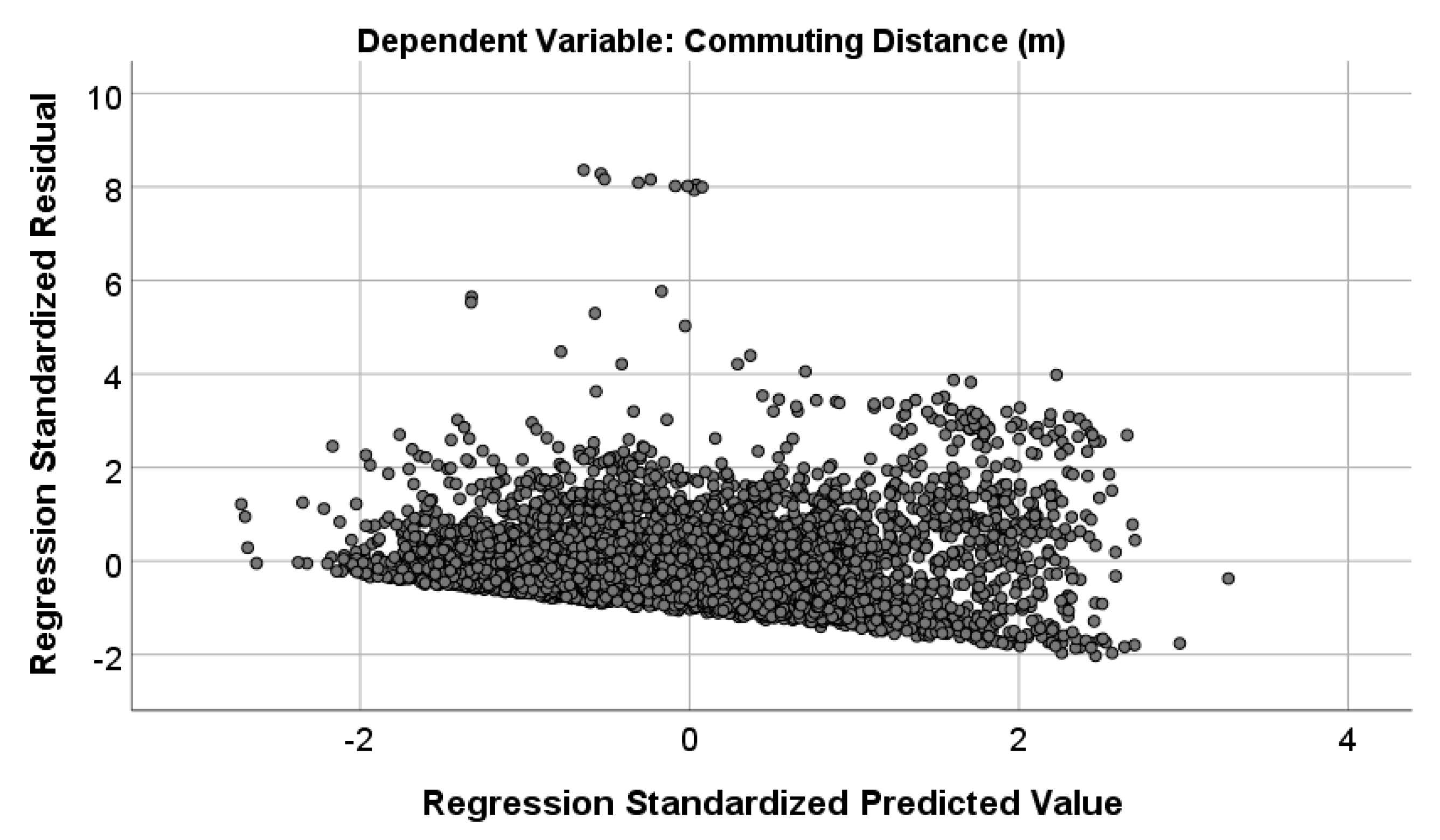
In order to answer the first research question of this study, the weighted least squares (WLS) method was applied to model commuting distances. WLS was applied because of the existence of heteroscedasticity in the commute distance variable. This problem was detected by checking the overall distribution of the variable and using four heteroscedisticity tests. The general controlling of the distribution shows a clear heteroscedasticity problem in the distribution (Figure 2). However, to confirm the existence of the problem, heteroscedisticity tests were applied to the commute distance variable in a univariate linear regression, with all the continuous variables as covariates. We used the White test (chi-square = 305.2, df = 166, p < 0.001), modified Breusch–Pagan test (chi-square = 65.5, df = 1, p < 0.001), Breusch–Pagan test (chi-square = 431.4, df = 1, p < 0.001), and F Test for heteroscedasticity (Chi-square = 66.5, df = 1, p < 0.001). The results of all four tests highly significantly reject the null hypothesis of the homoscedasticity of the distribution. Thus, WLS was applied instead of ordinary least squares (OLS).

The dependent variable was the commute distance measured by meter. Twenty-four variables were chosen as explanatory variables at the first step and a preliminary model was generated using SPSS version 25. The modeling was conducted in 6 iterations, in each of which one or two variables with the highest p-values were eliminated from the model to reach the highest R². The 6th model that included 14 explanatory variables generated the best results, including pseudo R² and significance of variables. The most important eliminated variables were gender, household monthly living costs, shopping-entertainment mode choice in neighborhood, shopping-entertainment mode choice outside neighborhood, and intersection density. The significance levels were 0.05 and the weights were allocated to the dependent variable (commute distances) ranging from −2 to 2 by in-between steps of 0.5 each. The WLS models included continuous and dummy variables. The continuous variables were kept as they were after data calibration and validation. The dummy variables were generated by coding categorical variables.

Table 2. Descriptive statistics of the continuous variables of the Weighted Least Squares (WLS) models.

Variable	n	Range	Minimum	Maximum	Mean	Std. Deviation
Household Car Ownership	7667	11	0	11	0.97	0.795
No. of Driving Licenses in Household	7832	8	0	8	1.79	1.120
Average Monthly Household Income (Euro)	8045	70,000	0	70,000	4094.11	4525.178
Frequency of Commute Trips	7154	70	0	70	10.61	6.409
No. of Non-Work Activities in the Last Week	7735	30	0	30	3.02	2.584
Last Relocation Time	8210	87	0	87	15.15	11.800
Commuting Distance (m)	5123	77,106	0	77,106	8824.79	8661.345
Link-Node Ratio	8097	1.723	1.110	2.833	1.56523	0.211771
Street Length Density (m/ha)	8098	553.7	92.3	646.1	303.965	75.4597
No. of Accessed Facilities	8097	55	0	55	12.77	9.399
Access to Facilities (m)	8087	3313	633	3946	1355.96	452.935

illustrates the descriptive statistics of the continuous explanatory variables.

Table 3. Categorical variables of the WLS models.

Variable	Category		n	%	Valid%
Individual Driving License Ownership	Valid	No	3483	42.3	42.3
		Yes	4743	57.6	57.7
		Total	8226	99.9	100.0
	No Response		11	0.1
	Total		8237	100.0
Commute Mode Choice	Valid	No Personal Car	7012	85.1	85.1
		Personal Car	1225	14.9	14.9
		Total	8237	100.0	100.0
Frequency of Public Transit Trips	Valid	Non-Frequent Use	2925	35.5	35.6
		Frequent Use	5280	64.1	64.4
		Total	8205	99.6	100.0
	No Response		32	0.4
	Total		8237	100.0
Entertainment Place	Valid	Inside Neighborhood	3193	38.8	39.0
		Farther Places	5002	60.7	61.0
		Total	8195	99.5	100.0
	No Response		42	0.5
	Total		8237	100.0

summarizes the frequencies of the dummy variables. To code commute mode choice, all the selected options were coded into car and no-car use. The five categories of public transit use frequency were coded into two dummy categories of frequent and non-frequent public transit use. Frequent use includes everyday use and some uses per week, while non-frequent use includes some ridership per month, rarely, and almost never. For coding the place of entertainment, the places were used as they were given by respondents during the interviews. The places were categorized into two dummy categories of inside the neighborhood and farther places including all the places outside the neighborhood or in the city center, etc.

Table 4. Variables and quantification methods.

Variable	Code	Type	Unit	Quantification Method
Individual driving license	IndLic	Continuous	-	Owning a driving license by the respondent (yes, no).
Household car ownership	HouseCO	Continuous	-	The number of personal cars owned by the household members.
Average household monthly income	HouseIncome	Continuous	-	The household average monthly income reported by the respondent.
Frequency of commute trips	FreqComTrip	Continuous	-	Respondent’s frequency of commute trips during the seven days before the interview.
Commute mode choice	CommuteMC	Dummy	-	The dominant commute mode choice of the respondent (car, no car).
Number of non-work activities	NonWorkAct	Continuous	-	Respondent’s frequency of non-work activities during the seven days before the interview.
Shopping/entertainment place	ShopEntPlace	Dummy	-	The dominant place of shopping and entertainment of the respondent (neighborhood, outside neighborhood/farther).
Presence of attractive shops or shopping centers in the neighborhood	AttractiveShop	Dummgy	-	Presence of attractive shops or shopping centers in the neighborhood where the respondent lives (yes, no).
Frequency of public transportation use	FreqPT	Dummy	-	The frequency of the respondent’s public transit use coded from categorical to dummy (frequent user: every day or sometimes per week, or non-frequent user: sometimes per month, rarely, and almost never).
Entertainment place	EntPlace	Dummy	-	The dominant place of entertainment of the respondent (neighborhood, outside neighborhood/farther).
Last relocation	LastRelocation	Continuous	-	The years passed from the last house relocation.
Link-node ratio	LinkNodeRat	Continuous	-	The number of links (street segments) divided by nodes (street intersections) of the street network within 600-m catchment area (based on the network) of each of the respondents’ homes. Calculations were done for areas inside the neighborhood boundary or outside. This indicator evaluates the typology of intersections (i.e., four- and five-way intersections get higher values than three-way intersections). Values of 1.4 and higher indicate good connectivity.
Street-length density	StreetLengthDen	Continuous	m/ha	The length of streets divided by the area of the 600-m catchment area (based on the network) of the respondents’ homes. Calculations were done for areas inside the neighborhood boundary or outside. Higher densities indicate better connectivity.
No. of accessed facilities	AccTotalCount	Continuous	-	The number of neighborhood public facilities within a 600-m catchment area (based on the network) of the respondents’ homes. The facilities included five types: bakeries, clinics and other medical centers, mosques, parks, and schools.
Access to neighborhood facilities	AccTotal	Continuous	meter	The average distance (based on the network) from each respondent’s home to neighborhood public facilities within the neighborhood or located within a linear 600-m buffer (like the crow flies) outside the neighborhood boundary. The facilities included five types: bakeries, clinics and other medical centers, mosques, parks, and schools.

summarizes the variables and their quantification methods. Regressing work trip lengths on a variety of explanatory variables covering socio-demographics and urban form have already been applied in a number of studies [36,37].

To answer the second research question, the same 14 explanatory variables were taken for the city models, so that they were comparable with the MENA model as well as with one another. The WLS modeling and weighting were conducted with the same procedure. Finally, the commute distances of the three case-study cities were descriptively analyzed, and analysis of variance was conducted, with the null hypothesis that the mean of commute distances of the working respondents of Tehran, Istanbul, and Cairo were the same. In order to compare the mean commuting lengths across the three cities, the independent-sample Kruskal–Wallis test was applied. The null hypothesis of this test was that the mean rank commute distances of the cities were the same.

Since there were considerable numbers of independent variables in the models, the possible problem of multicollinearity was checked for using the collinearity diagnostics tool in SPSS. In the outputs, when variance inflation factor (VIF) values were less than 3, it was assumed that there is no multicollinearity problem, while when they were more than 3, it was probable that collinearity existed. Moreover, when the VIF values were more than 5, it was likely that there was collinearity and when they were more than 10, there was definitely collinearity.

4. Findings

4.1. Determinants of Urban Commute Distance in Base Cities

In order to determine commute distances, one WLS model was produced for the overall sample of 8237 individuals in the three cities.

Table 5. The WLS model for the Middle East and North Africa (MENA) region including the coefficient estimates and F-test results (R² = 0.297).

ANOVA	Measure	Sum of Squares		df	Mean Square	F	p-Value
	Regression	1272.626		15	84.842	120.262	<0.001
	Residual	3012.374		4270	0.705	-	-
	Total	4285		4285	-	-	-
Coefficients	Category	B	Std. Error	Beta	Std. Error	t	p-Value
	IndLic	297.438	29.069	0.236	0.023	10.232	<0.001
	HouseCO	229.135	34.688	0.255	0.039	6.606	<0.001
	HouseIncome	0.025	0.008	0.111	0.038	2.959	0.003
	FreqComTrip	24.724	3.756	0.334	0.051	6.582	<0.001
	CommuteMC	−361.573	74.986	−0.094	0.019	−4.822	<0.001
	NonWorkAct	−23.847	11.554	−0.062	0.030	−2.064	0.039
	ShopEntMCIn	506.199	98.500	0.086	0.017	5.139	<0.001
	AttractiveShop	257.627	40.926	0.140	0.022	6.295	<0.001
	FreqPT	274.317	36.624	0.211	0.028	7.490	<0.001
	EntPlace	−178.347	34.968	−0.179	0.035	−5.100	<0.001
	LastRelocation	−13.132	1.171	−0.552	0.049	−11.218	<0.001
	LinkNodeRat	−688.935	60.525	−1.417	0.125	−11.383	<0.001
	StreetLengthDen	1.062	0.225	0.506	0.107	4.721	<0.001
	AccTotalCount	18.084	2.033	0.265	0.030	8.894	<0.001
	AccTotal	0.601	0.047	0.703	0.055	12.684	<0.001

shows the model outputs and the related F-test results. As explained in the methodology section, the insignificant variables were eliminated until the best organization of variables was found. The final model includes 15 highly significant (p < 0.01) or significant (0.01 < p < 0.05) variables including individual driving license, household car ownership, household monthly average income, frequency of commute trips, commute mode choice, frequency of non-work activities, shopping-entertainment mode choice in the neighborhood (short trips), presence of attractive shops in the neighborhood, frequency of public transit use, entertainment place, the years passed since the last house relocation, link-node ratio, street length density, number of accessible facilities within the catchment areas of the house, and distance to access facilities within the catchment area. With the exception of the number of non-work activities (p = 0.039), all of the other variables are highly significant. The results of the multicollinearity diagnostics show that the VIF values of all independent variables are between 1 and 1.6, which indicates no multicollinearity. The exception is intersection density, which shows a VIF value of 3.07. Since the amount is slightly higher than the threshold of 3 for probable collinearity, the variables are kept in the model and it is assumed that this very tiny indication of collinearity does not affect the whole model.

Three individual and household variables of individual driving license, household car ownership, and household income are strongly positively associated with commute length, with β ranging from 0.111 to 0.255. Mobility habits and decisions are also important in this model. Commute mode choice is negatively associated, meaning that, for individuals who commute longer distances, a nine percent increase in their personal car use is expected (using a car was coded 1 and all other modes were coded 0). However, the mode choice related to shopping and entertainment is positively correlated with commuting length. This indicates the different nature of mode choices for different purposes. Spatial activities and perceptions also have their own place in the model. Having entertainment outside of the living neighborhood is associated with having shorter commute trips (β = −0.179). Those passengers who feel there are attractive shops in their neighborhood are more likely to commute longer distances (β = 0.140). Living in houses for a long time is not associated with longer commuting distance (β = −0.552).

The strongest correlation is related to urban form, namely link-node ratio. Link-node ratio around the home is negatively associated with commuting distance (β = −1.417), while intersection density per area was already eliminated from the equation because of insignificance. The significance of link-node ratio in this model reflects the importance of street network connectivity around the origin. The second-most important significant variable is also related to land use traits. The average distance to five neighborhood amenities (bakeries, schools, urban parks and green spaces, religious buildings, and medical buildings) are positively correlated to commute length (measured by meter). Likewise, street length density around the living place is positively associated with commute lengths. This unexpected positive correlation of link-node ratio and street length density can be explained by the city-level models. Frequent public transit use is also correlated with longer commuting distance (β = 0.211).

The results of analysis of variance (ANOVA) indicates that the model is valid (p < 0.001). The R² is 0.297, which indicates that around one-third of the variance in commute distance has been explained by the model (Table 5). The multiple R has a value of 0.545.

4.2. Differences between the Commute Distances of the Three Cities

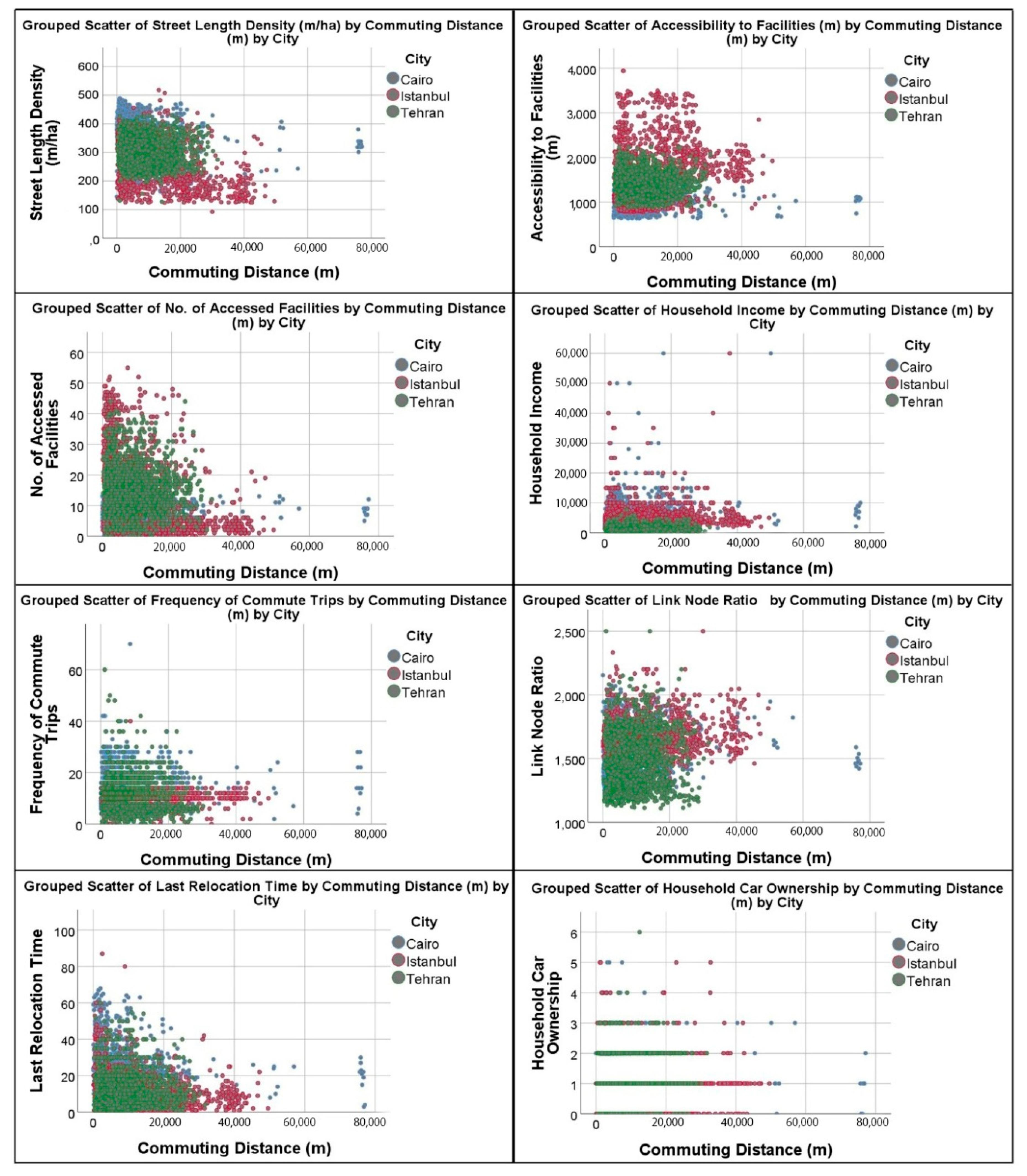
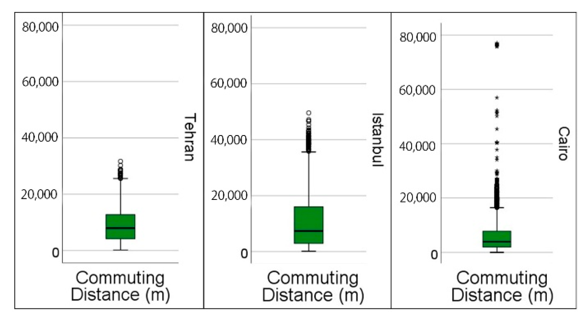
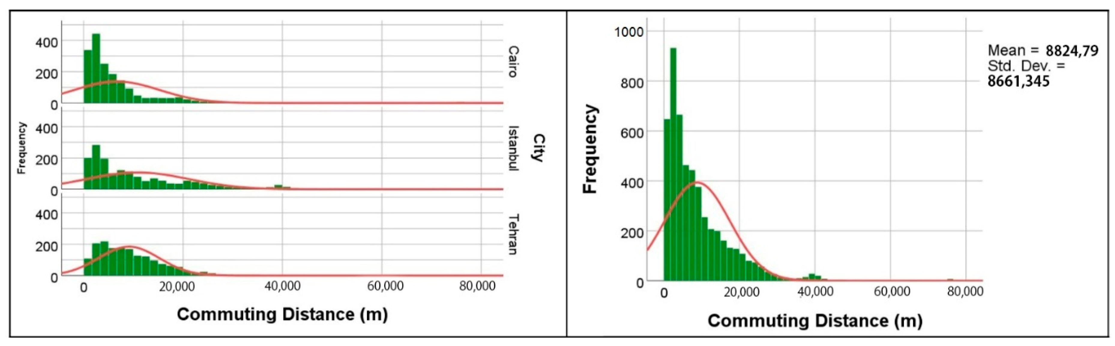
Figure 3 shows the value of continuous data and one of the categorical variables separately for each city. The mean commuting distance for the overall sample of the three cities is 8825 m (Table 1). Since the data have a non-normal distribution, T-tests were not applied to test the significant difference between the commute distances of the three cities. The results of the independent-sample Kruskal–Wallis test reject the null hypothesis of equality of mean ranks of commute distance across the three cities (statistic = 327.823, df = 2, significance level = 0.05); thus, the distances are significantly different among the cities. This result indicates that the commute distances in Tehran (n = 1691, mean = 9096 m), Istanbul (n= 1664, mean = 10839 m), and Cairo (n = 1768, mean = 6670 m) are significantly different. The results of the analysis of variance, which is less sensitive to violation of the normality assumption compared to the T-test, confirm the results of the Kruskal–Wallis test (df = 2, F = 104.604, p < 0.001). Figure 4 and Figure 5 depict the commuting distances in the three cities and the whole sample.

4.3. City-Level Comparison of Commute Trip Determinants

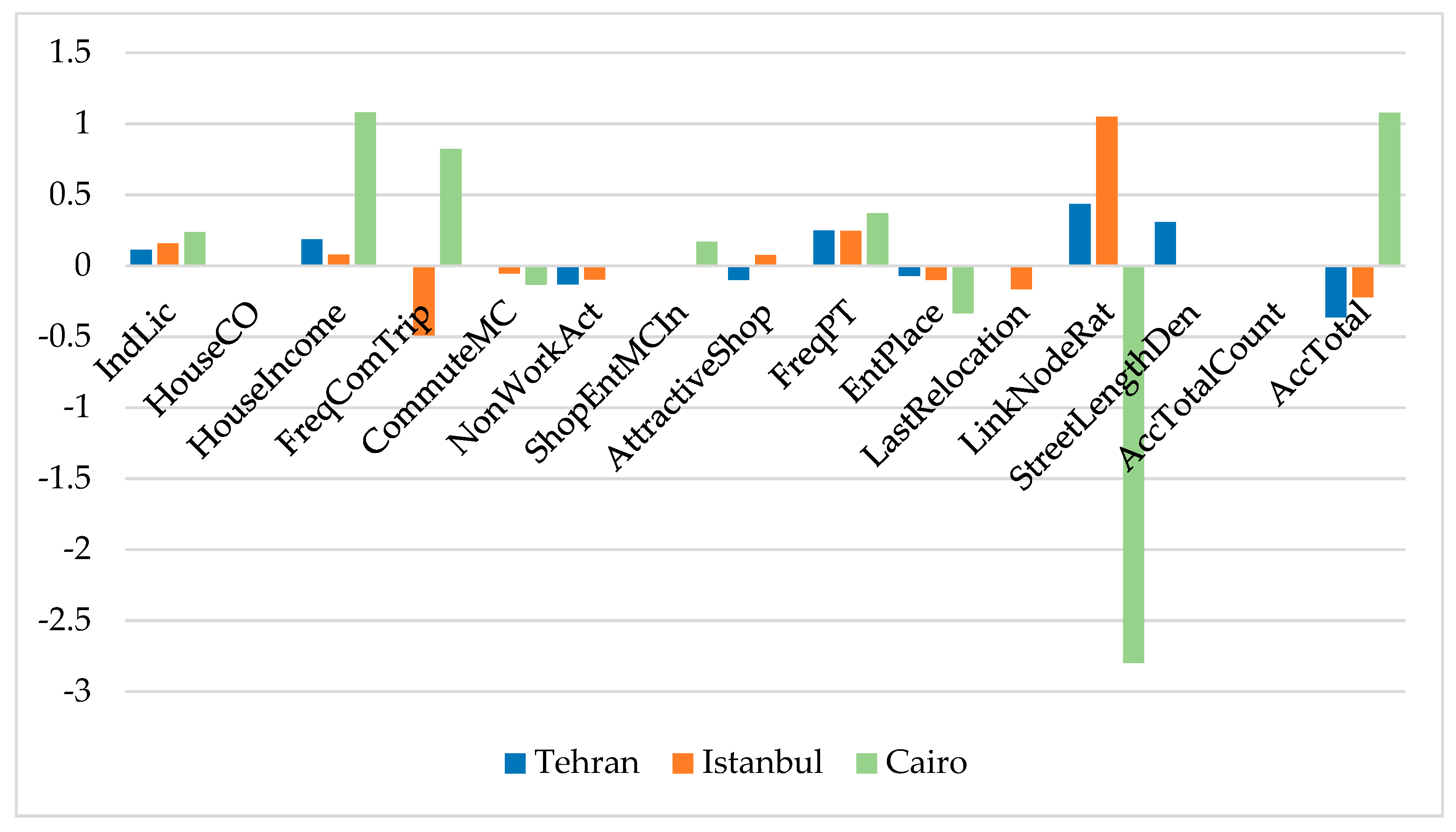
To understand the main reasons behind the differences between the commute distances of the cities, the same modeling procedure and variable organization used for the overall sample were applied to separate datasets of the three case-study cities. Such a modeling approach made inter-city comparisons easier. The results of separate modeling for the three cities are seen in

Table 6. WLS model estimates for Tehran, Istanbul, and Cairo.

Category	B	Std. Error	Beta	Std. Error	t	p-Value
Tehran
IndLic	566.957	215.094	0.112	0.043	2.636	0.008
HouseCO	129.595	159.958	0.038	0.047	0.810	0.418
HouseIncome	0.579	0.134	0.186	0.043	4.318	<0.001
FreqComTrip	−8.682	12.722	−0.026	0.038	−0.682	0.495
CommuteMC	392.151	281.241	0.048	0.035	1.394	0.163
NonWorkAct	−119.469	33.991	−0.132	0.037	−3.515	<0.001
ShopEntMCIn	282.973	258.229	0.030	0.027	1.096	0.273
AttractiveShop	−600.524	193.699	−0.100	0.032	−3.100	0.002
FreqPT	1580.281	227.239	0.249	0.036	6.954	<0.001
EntPlace	−368.870	205.227	−0.071	0.040	−1.797	0.072
LastRelocation	7.399	9.825	0.025	0.033	0.753	0.452
LinkNodeRat	1315.310	289.352	0.436	0.096	4.546	<0.001
StreetLengthDen	4.402	2.317	0.307	0.162	1.900	0.058
AccTotalCount	1.414	14.012	0.005	0.053	0.101	0.920
AccTotal	−1.077	0.457	−0.363	0.154	−2.356	0.019
Istanbul
IndLic	402.158	86.627	0.158	0.034	4.642	<0.001
HouseCO	−20.158	71.348	−0.012	0.041	−0.283	0.778
HouseIncome	0.025	0.014	0.078	0.042	1.843	0.065
FreqComTrip	−75.132	16.755	−0.490	0.109	−4.484	<0.001
CommuteMC	−249.554	128.783	−0.055	0.028	−1.938	0.053
NonWorkAct	−49.837	17.873	−0.096	0.034	−2.788	0.005
ShopEntMCIn	198.672	332.521	0.015	0.025	0.597	0.550
AttractiveShop	154.898	82.101	0.074	0.039	1.887	0.059
FreqPT	538.080	85.530	0.244	0.039	6.291	<0.001
EntPlace	−210.434	77.168	−0.100	0.037	−2.727	0.006
LastRelocation	−15.004	3.529	−0.164	0.039	−4.252	<0.001
LinkNodeRat	1091.533	266.110	1.049	0.256	4.102	<0.001
StreetLengthDen	0.730	0.875	0.128	0.154	0.834	0.404
AccTotalCount	−6.188	5.724	−0.086	0.080	−1.081	0.280
AccTotal	−0.250	0.138	−0.223	0.123	−1.812	0.070
Cario
IndLic	171.887	44.149	0.237	0.061	3.893	<0.001
HouseCO	−14.812	52.766	−0.029	0.102	−0.281	0.779
HouseIncome	0.144	0.015	1.080	0.112	9.661	<0.001
FreqComTrip	34.619	5.210	0.823	0.124	6.645	<0.001
CommuteMC	−375.717	129.456	−0.135	0.046	−2.902	0.004
NonWorkAct	−15.482	23.188	−0.061	0.091	−0.668	0.504
ShopEntMCIn	670.891	150.888	0.168	0.038	4.446	<0.001
AttractiveShop	60.818	82.580	0.049	0.066	0.736	0.462
FreqPT	281.220	55.086	0.371	0.073	5.105	<0.001
EntPlace	−190.206	49.404	−0.336	0.087	−3.850	<0.001
LastRelocation	−0.988	2.180	−0.077	0.170	−0.453	0.650
LinkNodeRat	−765.112	88.902	−2.799	0.325	−8.606	<0.001
StreetLengthDen	0.448	0.304	0.387	0.263	1.473	0.141
AccTotalCount	−8.281	8.405	−0.176	0.179	−0.985	0.325
AccTotal	0.582	0.159	1.077	0.293	3.670	<0.001

. The WLS model for Tehran indicates that nine variables are significant (p < 0.05) or marginally significant (0.05 < p <0.10). Seven variables, namely individual driving license, household income, number of non-work activities, frequency of public transit use, link-node ratio around the living place, and walkable distance to neighborhood facilities, are significantly related to commute distance. Moreover, entertainment place and street-length density are marginally significant. Likewise, in Istanbul, seven variables are significantly correlated with commute length: individual driving license, frequency of commute trips, entertainment place, number of non-work activities, frequency of public transport use, link-node ratio, and the time passed since the last house relocation. Additionally, four variables, namely household income, commute mode choice, presence of attractive neighborhood shops, and walkable distance to neighborhood facilities are marginally significantly associated with commute distances. In Cairo, nine variables, namely of individual driving license, household income, frequency of commute trips, commute mode choice, mode choice of shopping and entertainment, frequency of public transit use, entertainment place, link-node ratio, and walkable distance to neighborhood facilities, are highly significant.

The commute trip models of Tehran and Istanbul look very similar, while Cairo looks slightly different. Six variables, namely individual driving license, household income, commute mode choice, frequency of public transit use, entertainment place, and link-node ratio, are significant or marginally significant in the models of all three cities. Number of non-work activities and presence of attractive shops in the neighborhood are important in Tehran and Istanbul but not in Cairo. Commute mode choice and frequency of commuting are only important in Istanbul and Cairo. The time passed from the last relocation is only important in Istanbul, while street-length density is only important in Tehran. The significant standardized coefficients (β) of the variables of the three cities have been clustered in Figure 6 for easier comparison. In general, the models of Tehran and Istanbul are more similar (see Table 6 and Figure 6). The results of F-test (

Table 7. F-test results of WLS models of Tehran, Istanbul, and Cairo.

Area	Tehran (R² = 0.465, Multiple R = 0.682)					Istanbul (R² = 0.329, Multiple R = 0.574)					Cairo (R² = 0.355, Multiple R = 0.596)
Category	Sum of Squares	df	Mean Square	F	p-Value	Sum of Squares	df	Mean Square	F	p-Value	Sum of Squares	df	Mean Square	F	p-Value
Regression	59,335	15	3956	81.8	<0.001	541	15	36	53.2	<0.001	431	15	28.7	44	<0.001
Residual	68,244	1412	48.3			1104	1630	0.68			782	1198	0.65
Total	127,579	1427				1645	1645				1213	1213

) show that the models are all valid (p < 0.001) and a moderate amount of variance is explained by the city models. The R² values for Tehran, Istanbul, and Cairo are 0.465, 0.329, and 0.355, respectively. These results are almost similar to the those of other works on commute distance, e.g., the results of Manaugh et al. and Miller and Ibrahim [17] are higher than the R-squares of Lee and McDonald [19] and Næss, Strand, Wolday, and Stefansdottir [38]. These R-squares are equal to or higher than those of some of the other models in urban transportation planning [39,40,41].

5. Discussion

5.1. Contextual Differences with High-Income Countries

The major discovery about the differences between the predictors of commuting distance in the MENA cities and those of high-income cities is that age and gender are not significant in MENA, but, as we saw in the literature review, they are significant in the Netherlands [18,22,42] and Canada [23,24]. This study’s findings relating to age and gender are in line with the results of Næss et al. [38], who found these two variables insignificant in Oslo, Norway. Like age and gender, the results of commute mode choice are not exactly parallel with the western findings. According to Chatman [39], commuting distance is a marginally significant predictor of choosing a car for commuting in US cities (p = 0.087).

The MENA model shows that commute mode choice is highly significantly associated with commuting distance; however, not all of the three cities show this significance. This variable is not a predictor in Tehran (p = 0.163). In Istanbul, it has marginal significance (p = 0.053), but in Cairo, it is highly significant (p < 0.001). Previous studies confirm that commuting distance and mode choice are correlated in the Netherlands [31,43,44]. The results of this study about the correlation of commute mode choice with commute distance are in line with the Canadian findings. Nevertheless, none of the other significant predictors in the MENA cities are similar to those of Canada, which assert that “sex, age, occupation type, mode of transportation, migration, employment status, mixed land uses, and job concentration at the place of residence of the worker all explain commute distance.” [33].

Household income and household car ownership are important in the MENA context, as they are in Montréal, Canada, and Northern Ireland [20]. Car ownership is highly significant in the car and walk/bike commute distance model of Dutch cities, but it is not correlated with public transit trip length. Income highly significantly predicts commute trip length by car, public transportation, and walking/biking [40]. However, in Oslo, Norway, individual income is not a significant variable [38].

This study applied the residential location choice in the form of the time passed since the last relocation of the household. This refers to the mobility biographies of the household; if a relatively long time has passed since the last relocation, it might mean that, during this time, the job or main activity of the respondent may have changed, so this variable may be related to his/her current commute distance. Like in the MENA region, residential location choices are important in defining commute distances in San Francisco, USA [19]. The results of this study are also in line with the findings of other scholars, who found relationships between non-work activities and commute travel by all modes, particularly by bike. In the MENA regions, non-work variables such as entertainment place, shopping/entertainment mode choice, number of non-work activities, and presence of attractive shops in the neighborhood are associated with commuting length [45,46,47].

The urban form variables of this study were developed on a disaggregate basis, so the researchers were not restricted by census data organization and form, but most of the studies that are taken for comparison had this limitation. Thus, the consequence is that the land use variables of this study cannot easily be found in other studies. However, from a wider perspective, it is observable that some of the urban form variables, such as link-node ratio, walkable accessibility to neighborhood facilities, and the number of the accessible facilities, are correlated with commute trip distance, as several land use and spatial variables are important in western countries [36,37,38,42,48].

This study also applied some variables in the models that were not examined in previous studies, e.g., the perceptions and attachment of the respondent regarding his/her neighborhood is important in the MENA region, but such evidence is not available in the existing literature. As a summary of this sub-section, it can be concluded that urban commute distances may have some differences in different contexts, including different countries and regions of the world; in other words, urban commute distances are relatively context-sensitive. This is consistent with Schwanen and Páez’s discussion about the contextuality of urban travel behavior [49]. This hypothesis is strengthened even more by highlighting the contextual differences between MENA countries and other developing countries or emerging markets. For instance, age and gender are not significant in MENA, but in Kumming, China, gender is correlated with commute distance while age is not [50]. These two important variables are positively associated with commute length in the Gauteng City region in South Africa [51]. The main reason behind the context-specificity of the travel behaviors and decisions in MENA is the differences between the culture, geography, history, religion, etc., in the region from those of high-income countries or other developing regions. These issues affect all behaviors, including travel behaviors, according to the theory of planned behavior. It is not surprising that travel behaviors are different in the Middle East from other developing regions like South America. The idea of the context-sensitivity of travel behaviors rejects the highly common trend of policymaking based on basic studies of travel behaviors in other regions of the world.

5.2. Urban Planning Policy Implications for MENA Cities

Although there is evidence that socio-economic traits may play a stronger role than the built environment in defining urban travel behavior in some of the cities of the MENA region [52,53], but when focusing on only work travels, the role of land use and especially urban form characteristics related to employment around destinations may be proven as effective. As a result of technical difficulties and limitations of resources, the land use within walking distance around workplaces was not quantified in this study, and only the urban form of the origins was applied in the models. Apart from such limitations, the larger MENA cities can use the results of this study to shorten commute distances, which will have an effect on commute mode and time. This may be implemented by the long-term transformation of land use, especially by increasing the connectivity of street networks by increasing link-node ratios. The very high negative coefficient of link-node ratio in Cairo (β = −2799) suggests that this strategy can be much more effective in determining the correlates of commuting distance in this city. Moreover, the allocation of more shops and entertainment functions in urban development plans and making the local shops and shopping malls more attractive can affect commute distance in the long term in Cairo. This affects commute lengths in combination with non-work activities and trips. Egyptian planners can particularly increase attractive local shops and expect to affect commute distances in Cairo. The results of this study suggest that, if non-work facilities such as shopping and leisure amenities are strengthened and the non-work activities of residents are increased in Cairo, commute distances are likely to decrease. In Tehran and Istanbul, providing a better distribution of local and neighborhood facilities including commercial and public functions may lead to a decrease in commuting distance.

According to the theory of planned behavior (TPB), interventions may be planned to affect urban travel behavior by targeting changes in attitudes, subjective norms, and perceptions and, as a consequence, urban travel behaviors [54]. This can be more effective when a change in a reasoned decision is targeted, e.g., mode choice can be a reasoned decision [55]. This paper claims that a very large share of the attitudes and perceptions of people stem from culture and context. Thus, changing the ways in which people decide about their mobility can be achieved by planning the physical environment based on local knowledge about both travel patterns and the relationship with the built environment. In order to plan mobility behaviors exemplified by commuting, the application of context-specific knowledge is necessary. In other words, the application of internationally accepted norms originating from western or high-income countries will not work for urban planning and mobility policymaking for the purpose of shortening commute distances.

The practical recommendations of this paper to urban planners with the purpose of decreasing commuting distances can be specific for each one or two cities of this study. These decision making and planning recommendations can be direct in nature (directly decreasing commute distance). These recommendations can be summarized as below:

Tehran: Increasing street network accessibility via shortening the street segment lengths by adding junctions and intersections. This will encourage the inhabitants of Tehran to use non-motorized non-work travel and decrease their commute distances.

Istanbul: Increasing the link-node ratio by adding to the streets of junctions, i.e., making more four and five-way intersections instead of three-way ones.

Cairo: Increasing the number of street segments versus intersections (increasing network connectivity). This can indirectly decrease commute trip lengths in relation to non-commute activities. This idea can be combined with the concept of pedestrianization and development of car-free areas to provide a preventive push factor for personal car use.

Cairo: Shortening the accessibility distances to neighborhood-level amenities like retail, shops, schools, bakeries, religious buildings, open/green spaces, and the like. The inhabitants of Cairo may shorten their commuting distances if they can carry out some of their non-work activities in the vicinity of their living place.

5.3. Study Limitations

As mentioned above, limitations of time and resources prevented the quantification of land use around workplaces from being included in this study. Apart from this deficiency, the population data were not available in the GIS base maps of the three case-cities; therefore, population densities could not be quantified in a disaggregate manner. Moreover, there is always a data-related problem in cities in developing countries in that there are usually limited data about the places of jobs and employment clusters. Thus, population and employment density variables could not be generated in this study. By resolving these problems in the future, more comparable results can be produced and better international knowledge can be presented to the urban transportation community.

6. Conclusions

This study employs a primary disaggregate dataset of a less-researched context, seeking to answer relevant mobility questions regarding determinants of urban commute travel length in this context. This makes the study novel and innovative in its geographical context. The sample size makes some of the biases that occurred during the data collection and analysis ignorable. The empirical results can be summarized in relation to the research questions as follows:

Fifteen highly significant or significant variables, including individual driving license, household car ownership, household monthly average income, frequency of commute trips, commute mode choice, frequency of non-work activities, shopping-entertainment mode choice in the neighborhood (short trips), presence of attractive shops in the neighborhood, frequency of public transit use, entertainment place, the years passed since last house relocation, link-node ratio, street length density, number of accessible facilities within the catchment areas of the house, and accessible distance to facilities within the catchment areas, predict the lengths of urban commute trips in the MENA sample including Tehran, Istanbul, and Cairo.

There is a significant difference between the mean commute travel distances in the three cities: Tehran: 9096 m, Istanbul: 10839 m, and Cairo: 6670 m.

Although there are differences between the determinants of commute trip distance in the three studied cities, the results of the models show that there are similarities between the cities. The commute trip length determinants of Tehran and Istanbul are highly similar. There are some differences between Cairo and the other two cities. Nevertheless, the findings show the effectiveness of individual/household factors and urban form characteristics in all three cities.

These findings show some differences with the findings of high-income societies, the most apparent of which is that, unlike western countries, age and gender are not significant predictors of urban commute distance in MENA large cities. Commute mode choices are only marginally significantly correlated with commute trip length in the USA, but this variable is highly significant in the three MENA cases of this study.

The significant determinants of the models presented in this research help urban planners and decision makers of the MENA region affect commute trips in the long term, using indicators like link-node ratio, distribution of local facilities, and walking distance to them. More complicated and detailed datasets and analysis methods can produce more robust results to support a shift towards more sustainable urban mobility in the region.

References

- Becker, G.S. A Theory of the Allocation of Time. Econom. J. 1965, 75, 493. [Google Scholar] [CrossRef] [Green Version]
- DeSerpa, A.C. A Theory of the Economics of Time. Econom. J. 1971, 81, 828. [Google Scholar] [CrossRef]
- Litman, T. Transportation cost and benefit analysis. Vic. Transp. Policy Inst. 2009, 31. [Google Scholar]
- Englin, J.; Shonkwiler, J.S. Modeling Recreation Demand in the Presence of Unobservable Travel Costs: Toward a Travel Price Model. J. Environ. Econom. Manag. 1995, 29, 368–377. [Google Scholar] [CrossRef]
- Frank, L.; Bradley, M.; Kavage, S.; Chapman, J.; Lawton, T.K. Urban form, travel time, and cost relationships with tour complexity and mode choice. Transportation 2008, 35, 37–54. [Google Scholar] [CrossRef]
- Higgins, C.D.; Sweet, M.N.; Kanaroglou, P.S. All minutes are not equal: Travel time and the effects of congestion on commute satisfaction in Canadian cities. Transportation 2017, 45, 1249–1268. [Google Scholar] [CrossRef]
- Evans, G.W.; Wener, R.E. Rail commuting duration and passenger stress. Health Psychol. Off. J. Div. Health Psychol. Am. Psychol. Assoc. 2006, 25, 408–412. [Google Scholar] [CrossRef] [Green Version]
- Künn-Nelen, A. Does Commuting Affect Health? Health Econom. 2016, 25, 984–1004. [Google Scholar] [CrossRef] [Green Version]
- Novaco, R.W.; Collier, C. Commuting Stress, Ridesharing, and Gender: Analyses from the 1993 State of the Commute Study in Southern California; Institute of Transportation Studies, University of California: Oakland, CA, USA, 1994. [Google Scholar]
- Sandow, E. Til Work Do Us Part: The Social Fallacy of Long-distance Commuting. Urban Stud. 2014, 51, 526–543. [Google Scholar] [CrossRef]
- Cervero, R.; Kockelman, K. Travel demand and the 3Ds: Density, diversity, and design. Transp. Res. Part D Transp. Environ. 1997, 2, 199–219. [Google Scholar] [CrossRef]
- Sultana, S.; Weber, J. The nature of urban growth and the commuting transition: Endless sprawl or a growth wave? Urban Stud. 2014, 51, 544–576. [Google Scholar] [CrossRef]
- Marcińczak, S.; Bartosiewicz, B. Commuting patterns and urban form: Evidence from Poland. J. Transp. Geogr. 2018, 70, 31–39. [Google Scholar] [CrossRef]
- Rietveld, P.; Zwart, B.; van Wee, B.; van den Hoorn, T. On the relationship between travel time and travel distance of commuters. Ann. Reg. Sci. 1999, 33, 269–287. [Google Scholar] [CrossRef] [Green Version]
- Richard, S. Travel From Home: An Economic Geography of Commuting Distances in Montreal. Urban Geogr. 2006, 27, 330–359. [Google Scholar]
- Gordon, P.; Kumar, A.; Richardson, H.W. The influence of metropolitan spatial structure on commuting time. J. Urban Econom. 1989, 26, 138–151. [Google Scholar] [CrossRef]
- Miller, E.; Ibrahim, A. Urban Form and Vehicular Travel: Some Empirical Findings. Transp. Res. Rec. J. Transp. Res. Board 1998, 1617, 18–27. [Google Scholar] [CrossRef]
- Schwanen, T.; Dieleman, F.M.; Dijst, M. Travel behaviour in Dutch monocentric and policentric urban systems. J. Transp. Geogr. 2001, 9, 173–186. [Google Scholar] [CrossRef]
- Lee, B.S.; McDonald, J.F. Determinants of Commuting Time and Distance for Seoul Residents: The Impact of Family Status on the Commuting of Women. Urban Stud. 2003, 40, 1283–1302. [Google Scholar] [CrossRef]
- Shuttleworth, I.; Lloyd, C. Analysing average travel-to-work distances in Northern Ireland using the 1991 census of population: The effects of locality, social composition, and religion. Reg. Stud. 2005, 39, 909–921. [Google Scholar] [CrossRef]
- Helminen, V.; Ristimäki, M. Relationships between commuting distance, frequency and telework in Finland. J. Transp. Geogr. 2007, 15, 331–342. [Google Scholar] [CrossRef]
- Ettema, D.; Schwanen, T.; Timmermans, H. The effect of location, mobility and socio-demographic factors on task and time allocation of households. Transportation 2007, 34, 89–105. [Google Scholar] [CrossRef] [Green Version]
- Mercado, R.; Páez, A. Determinants of distance traveled with a focus on the elderly: A multilevel analysis in the Hamilton CMA, Canada. J. Transp. Geogr. 2009, 17, 65–76. [Google Scholar] [CrossRef]
- Manaugh, K.; Miranda-Moreno, L.F.; El-Geneidy, A.M. The effect of neighbourhood characteristics, accessibility, home-work location, and demographics on commuting distances. Transportation 2010, 37, 627–646. [Google Scholar] [CrossRef]
- Antipova, A.; Wang, F.; Wilmot, C. Urban land uses, socio-demographic attributes and commuting: A multilevel modeling approach. Appl. Geogr. 2011, 31, 1010–1018. [Google Scholar] [CrossRef]
- Boussauw, K.; Neutens, T.; Witlox, F. Relationship between spatial proximity and travel-to-work distance: The effect of the compact city. Reg. Stud. 2012, 46, 687–706. [Google Scholar] [CrossRef]
- Prashker, J.; Shiftan, Y.; Hershkovitch-Sarusi, P. Residential choice location, gender and the commute trip to work in Tel Aviv. J. Transp. Geogr. 2008, 16, 332–341. [Google Scholar] [CrossRef]
- Sheng, M.; Wu, W.; Gu, C. Commuting distance of rural migrants in urban China: The role of educational attainment. Sociol. Mind 2015, 5, 276. [Google Scholar] [CrossRef] [Green Version]
- Tkocz, Z.; Kristensen, G. Commuting distances and gender: A spatial urban model. Geogr. Anal. 1994, 26, 1–14. [Google Scholar] [CrossRef]
- Östh, J.; Lindgren, U. Do changes in GDP influence commuting distances? A study of Swedish commuting patterns between 1990 and 2006. Tijdschr. Voor Econ. En Soc. Geogr. 2012, 103, 443–456. [Google Scholar] [CrossRef]
- Van Acker, V.; Witlox, F. Commuting trips within tours: How is commuting related to land use? Transportation 2011, 38, 465–486. [Google Scholar] [CrossRef]
- Axisa, J.J.; Newbold, K.B.; Scott, D.M. Migration, urban growth and commuting distance in Toronto’s commuter shed. Area 2012, 44, 344–355. [Google Scholar] [CrossRef]
- Maoh, H.; Tang, Z. Determinants of normal and extreme commute distance in a sprawled midsize Canadian city: Evidence from Windsor, Canada. J. Transp. Geogr. 2012, 25, 50–57. [Google Scholar] [CrossRef]
- Masoumi, H.; Fruth, E. Transferring Urban Mobility Studies in Tehran, Istanbul, and Cairo to Other Large MENA Cities: Steps toward Sustainable Transport. Urban Dev. Issues 2020, 65, 27–44. [Google Scholar] [CrossRef]
- Masoumi, H.E.; Gouda, A.A.; Layritz, L.; Stendera, P.; Matta, C.; Tabbakh, H.; Fruth, E. Urban Travel Behavior in Large Cities of MENA Region: Survey Results of Cairo, Istanbul, and Tehran; Technische Universität Berlin: Berlin, Germany, 2018. [Google Scholar]
- Levinson, D.M.; Kumar, A. Density and the Journey to Work. Growth Chang. 1997, 28, 147–172. [Google Scholar] [CrossRef]
- Sun, X.; Wilmot, C.; Kasturi, T. Household Travel, Household Characteristics, and Land Use: An Empirical Study from the 1994 Portland Activity-Based Travel Survey. Transp. Res. Rec. J. Transp. Res. Board 1998, 1617, 10–17. [Google Scholar] [CrossRef]
- Næss, P.; Strand, A.; Wolday, F.; Stefansdottir, H. Residential location, commuting and non-work travel in two urban areas of different size and with different center structures. Prog. Plan. 2017, 128, 1–36. [Google Scholar] [CrossRef] [Green Version]
- Chatman, D. How Density and Mixed Uses at the Workplace Affect Personal Commercial Travel and Commute Mode Choice. Transp. Res. Rec. J. Transp. Res. Board 2003, 1831, 193–201. [Google Scholar] [CrossRef] [Green Version]
- Dieleman, F.M.; Dijst, M.; Burghouwt, G. Urban Form and Travel Behaviour: Micro-level Household Attributes and Residential Context. Urban Stud. 2002, 39, 507–527. [Google Scholar] [CrossRef]
- Krizek, K.J. Residential Relocation and Changes in Urban Travel: Does Neighborhood-Scale Urban Form Matter? J. Am. Plan. Assoc. 2003, 69, 265–281. [Google Scholar] [CrossRef]
- Schwanen, T.; Dieleman, F.M.; Dijst, M. The impact of metropolitan structure on commute behavior in the Netherlands: A multilevel approach. Growth Chang. 2004, 35, 304–333. [Google Scholar] [CrossRef]
- Schwanen, T.; Dijst, M.; Dieleman, F.M. A Microlevel Analysis of Residential Context and Travel Time. Environ. Plan. A Econ. Space 2002, 34, 1487–1507. [Google Scholar] [CrossRef]
- Susilo, Y.O.; Maat, K. The influence of built environment to the trends in commuting journeys in the Netherlands. Transportation 2007, 34, 589–609. [Google Scholar] [CrossRef]
- Bhat, C.R. Work travel mode choice and number of non-work commute stops. Transp. Res. Part B Methodol. 1997, 31, 41–54. [Google Scholar] [CrossRef] [Green Version]
- Lee, I.; Park, H.; Sohn, K. Increasing the number of bicycle commuters. Proc. Inst. Civ. Eng.Transp. 2012, 165, 63–72. [Google Scholar] [CrossRef]
- Park, H.; Lee, Y.J.; Shin, H.C.; Sohn, K. Analyzing the time frame for the transition from leisure-cyclist to commuter-cyclist. Transportation 2011, 38, 305–319. [Google Scholar] [CrossRef]
- Gordon, P.; Wong, H.L. The Costs of Urban Sprawl: Some New Evidence. Environ. Plan. A Econ. Space 1985, 17, 661–666. [Google Scholar] [CrossRef]
- Schwanen, T.; Páez, A. The mobility of older people : An introduction. J. Transp. Geogr. 2010, 18, 591–595. [Google Scholar] [CrossRef]
- He, M.; Zhao, S.; He, M. Determinants of Commute Time and Distance for Urban Residents: A Case Study in Kunming, China. In Proceedings of the 15th COTA International Conference of Transportation Professionals, Beijing, China, 24–27 July 2015; pp. 3663–3673. [Google Scholar]
- Geyer, H.S.; Molayi, R.S.A. Job-employed resident imbalance and travel time in Gauteng: Exploring the determinants of longer travel time. Urban Forum 2018, 29, 33–50. [Google Scholar] [CrossRef]
- Masoumi, H.E. Modeling the Travel Behavior Impacts of Micro-Scale Land Use and Socio-Economic Factors. TeMA-J. Land Use Mobil. Environ. 2013, 6, 235–250. [Google Scholar]
- Soltanzadeh, H.; Masoumi, H.E. The Determinants of Transportation Mode Choice in the Middle Eastern Cities: The Kerman Case, Iran. TeMA-J. Land Use Mobil. Environ. 2014, 7, 199–222. [Google Scholar]
- Ajzen, I. The Theory of Planned Behavior. Organ. Behav. Hum. Decis. Process. 1991, 50, 179–211. [Google Scholar] [CrossRef]
- Bamberg, S.; Ajzen, I.; Schmidt, P. Choice of travel mode in the theory of planned behavior: The roles of past behavior, habit, and reasoned action. Basic Appl. Soc. Psychol. 2003, 25, 175–187. [Google Scholar] [CrossRef]
Figure 1.
Illustration of linear commute distances in 18 neighborhoods in Tehran (top), Istanbul (middle), and Cairo (bottom) illustrated by aerial lines.
Figure 2.
Heteroscedasticity of the commute distances of the sample.
Figure 3.
Scatterplots of the continuous variables of the WLS model of the MENA region distributed according to commute travel distance, grouped by city.
Figure 4.
Comparative illustration of commute distances in Tehran, Istanbul, and Cairo.
Figure 5.
Distribution of commuting distances based on city (left) and the overall sample (right).
Figure 6.
The β values of the significant variables (including marginally significant at 0.1 level) of the WLS models of Tehran, Istanbul, and Cairo (dependent variable: commute distance).