The Efficacy of Allocating Housing Growth in the Los Angeles Region (2006–2014)


Department of Landscape Architecture and Regional Planning, UMass Amherst, Amherst, MA 01003, USA
Urban Sci. 2020, 4(3), 43; https://0-doi-org.brum.beds.ac.uk/10.3390/urbansci4030043
Submission received: 17 June 2020
/
Revised: 2 September 2020
/
Accepted: 5 September 2020
/
Published: 16 September 2020
Abstract
:California is known for home values that eclipse U.S. housing prices. To increase housing inventory, California has implemented a regional housing needs allocation (RHNA) to transmit shares of housing growth to cities. However, no study has established RHNA’s efficacy. After examining the 4th RHNA cycle (i.e., 2006–2014) for 185 Los Angeles region cities, this study determined that RHNA directed housing growth to the city of Los Angeles and the region’s outlying cities as opposed to increasing density in the central and coastal cities. Second, RHNA directed 62% of housing growth to the region’s unaffordable cities. Third, the sample suffered a 34% shortfall in housing growth due to the Great Recession but garnered an average achievement of approximately 93% due to RHNA’s transmission of minimal housing growth shares. Lastly, RHNA maintained statistically significant associations with increased housing inventory, housing affordability, and housing growth rates, indicating that RHNA may influence housing development.
1. Introduction
At WWII’s conclusion, many U.S. soldiers returned to a housing crisis. During the war, the building materials that would have supported housing construction were directed toward the war effort, and the prior migration of factory workers to cities exacerbated the limited housing choices [1,2]. In addition, the returning soldiers rapidly increased housing demand by forming new households, i.e., through marriage [3]. In response, Congress adopted the Housing Act of 1949. This act wove homeownership into the American dream by famously declaring, “the goal of a decent home and a suitable living environment for every American family” contributes to community development and advances “the growth, wealth, and security of the Nation” [4]. To purchase a home, however, many households must qualify for a mortgage.
In the United States, many real estate professionals employ a simple metric regarding mortgage qualification. Informally, a home’s selling price should be approximately equivalent to 2.6 times the homebuyer’s annual income [5]. By this informal qualification metric (IQM), the census data in Figure 1 indicates that the city of Los Angeles has not been affordable for quite some time. In 1980, the Los Angeles IQM was 6.1, whereas the national IQM was 2.8. By 2005, the Los Angeles IQM jumped to 12.0, over four times the national IQM of 3.6. Despite the Great Recession’s nationwide decline in home values, the Los Angeles IQM was still 9.3 in 2015, slightly less than 3 times the national IQM of 3.3.
Policy makers suggest two methods for increasing homeownership. First, the government could increase household purchasing power by providing a direct or indirect subsidy. Direct subsidies may operate as down payment assistance, whereas indirect subsidies may operate as tax deductions for mortgage interest and/or property taxes [6]. Second, the government could lower housing prices by encouraging housing construction. Encouragement may operate as the pre-emption of local restrictions (i.e., builder’s remedy) by higher-level governments (i.e., state courts) or by requiring that every city contains sufficient land to support housing construction [7,8]. Since 1969, California has taken an indirect approach by requiring that cities accommodate future housing construction because the state “recognizes that the most critical decisions regarding housing development occur at the local level” [9].
California’s intervention for encouraging housing construction is the regional housing needs allocation (RHNA). Since 1980, RHNA “establishes [a] minimum housing development capacity that cities and counties are to [accommodate] via their land use” [9]. California employs RHNA to increase regional housing inventory by allocating individual shares of housing growth to each city and county. RHNA strives for housing equity because the individual shares enumerate low-income and market-rate housing needs. Due to California’s home values, low-income housing targets households earning less than 120% of an area’s median income and spending less than 30% of their income on housing satisfaction. By contrast, market-rate housing is priced by the private sector. RHNA strives for housing diversity because the individual shares enumerate current and future housing needs. Current housing needs arise from delipidated and/or overcrowded units, whereas future housing needs arise from the formation of new households or the propensity that households will move to new communities.
Currently, California is embarking on its 6th RHNA cycle for the Los Angeles region (i.e., 2021–2029). In a series of letters, the state’s housing agency and the region’s council of governments tussled over who determines the region’s overall housing needs (i.e., 1.34 million units vs. 823,808 units, respectively) [10,11,12]. Due to revisions in state law, the housing agency prevailed. However, the allocation of individual shares to the region’s cities has not been finalized. In 1988, Baer raised the issue of equitable municipal effort in the RHNA process by asserting that California’s housing growth would be “foisted on to communities with considerable open space in which to expand,” while the “sins of the older, ‘built out’ communities” would be grandfathered in [13]. Thus, which cities should shoulder the burden of the region’s housing growth? In addition, no study has established whether RHNA has had any influence on housing construction, despite RHNA’s 40 year history.
This study proposes to assess RHNA’s efficacy by examining the allocation of housing growth during the 4th RHNA cycle for the Los Angeles region. Following this introduction, this paper discusses the origins of housing allocations, California’s approach to increase housing inventory, and the Great Recession. This paper then explains how maps and statistical analysis were employed to determine where RHNA directed housing growth, whether RHNA addressed housing affordability, which cities achieved their housing growth, and RHNA’s influence on housing inventory. While providing the results, this paper discusses the limitations of SCAG’s implementation of the Los Angeles region’s 4th RHNA cycle and ruminates on the upcoming 6th RHNA cycle. Finally, this paper discusses the implications of this study on metropolitan planning, housing affordability, and municipal effort.
2. Housing Allocations and California Housing Law
2.1. The Origins of Allocating Housing Needs
When Congress passed the Housing Act of 1949, one important provision was the expansion of the Federal Housing Administration (FHA). In 1934, Congress created the FHA to insure private residential mortgages in order to reduce a lender’s financial risk and ultimately stabilize housing markets during the Great Depression [14]. By 1949, the FHA would extend insurance to mortgages that conformed to FHA guidelines that maintained several discriminatory features [15]. First, mortgages could not be issued to neighborhoods with minority households due to redlining. Redlining is the practice of drawing red lines on maps around the neighborhoods in which the FHA would not insure mortgages [16]. Second, minority households could not receive FHA mortgages for a home in a white neighborhood. For white households, the FHA granted access to the middle class and the American dream [17]. For minority households, the FHA systematically limited residential choices and homeownership rates while also starving minority neighborhoods of capital [18].
In the mid-1960s, many urban cities erupted in riots. At that time, many U.S. central cities (e.g., Los Angeles, Baltimore, Detroit, Chicago, and Hartford) housed the nation’s minority and poor households. In its 1967 investigation of the riots, the Kerner Commission declared that if the issues of housing, employment, and education in urban areas were not addressed, then the U.S. would continue its path to two Americas, separate and unequal [19]. Consequently, Congress held hearings in 1968 to craft laws for making suburban communities amenable to accommodating low-income housing in order to resolve two interrelated issues: poverty and racial integration [20].
When it adopted the Housing and Development Act of 1968, Congress took a regional approach to connecting suburban housing opportunities with the housing needs of the central cities’ poor and minority households. Congress mandated that cities receiving section 701 funds for general plans must include a housing element that focuses on local and regional housing needs [21]. A housing element, which is a chapter in a city’s general plan, describes a city’s housing goals, programs, and objectives. Section 701 provided federal matching grants to cities in order to encourage local land-use planning [22]. As a lever, Congress tied federal infrastructure funds to suburban planning by using regional agencies as housing element evaluators. If a city’s housing element did not integrate low-income housing, then that city should be denied federal funds [23].
To overcome suburban resistance, one scholar advocated for metropolitan allocation systems. In 1967, Wheaton declared that “little of what is called comprehensive planning… is effective” because local plans simply ratify private market directives [24]. Wheaton also called out the federal government’s damaging role in abetting exclusionary zoning because federal housing programs had elevated the suburbs at the expense of inner cities. His solution was a metropolitan plan for allocating regional resources; however, he maintained several conditions that were designed not to upset suburban home rule. First, metropolitan planning occurs at the metropolitan scale. Second, metropolitan planning does not have the power to zone. Third, federal (not local) funds would implement metropolitan initiatives. In order to achieve equitable outcomes, two additional conditions were key: A low-density city would not be allowed to sequester high-paying jobs; school funding would be equalized to reduce property tax reliance and to prevent deficient school district operations.
In the early 1970s, metropolitan approaches filtered up to the U.S. Department of Housing and Urban Development (HUD). In 1971, HUD Secretary George Romney advocated for the elimination of urban and minority poverty by embracing the real city. Romney declared, “The impact of the concentration of the poor and minorities in the central city extends beyond the city boundaries to include the surrounding communities. The city and the suburbs together make up what I call the ‘real city.’ To solve problems of the ‘real city,’ only metropolitan wide-solutions will do” [25]. Simultaneously, many councils of government (COGs) and metropolitan planning organizations embraced the regional allocation of low-income housing needs. In 1970, for example, the Miami Valley Regional Planning Commission created a housing plan to “establish a housing database for the region, to project housing need, and to encourage [the] production” of public housing [26]. After Minnesota established the Metropolitan Council for the Minneapolis-St. Paul region in 1967, the council began to develop a fair-share plan to disburse subsidized housing away from the central city and to the suburbs by 1971 [26]. In 1972, the Southern California Association of Governments produced the Regional Housing Allocation Model in order “to guide the distribution of federal housing resources [and] aide local housing planning” in the Los Angeles region [9]. By 1976, Listokin identified over 45 regional and city plans that redistributed federal low-income housing programs, i.e., section 235—low-income homeownership, section 236—apartment owner mortgage subsidy, public housing [26].
Even though housing allocations extended the spirit of the Housing and Development Act of 1968, there was no explicit federal mandate supporting this approach [27]. Unlike housing elements, the housing allocations were implicitly implemented during a COG’s A-95 review. Thus, when Nixon issued his 1973 moratorium on public housing construction and the Housing and Community Development Act of 1974 directed low-income households to use housing vouchers, COGs began to implement fewer housing allocations [26]. Finally, when Reagan’s 1980s devolution slashed HUD budgets and terminated both Section 701 and the A-95 review, the enforcement of housing allocations ceased [8,28,29]. California’s housing allocations have persisted because RHNA was codified into the 1980 revision of the Housing Element Law [30]. This revision ushered in an era of regional governance in which the state housing agency, regional COGs, and cities work in tandem to increase housing inventory [31]. Under regional governance, the actors aspire to equal status; however, cities remain subordinate to the actions of the state and the COGs [32].
2.2. California’s Housing Element Law
Since 1969, California has required that cities and counties accommodate the housing needs of their residents. Accommodation means that every city must anticipate housing growth by planning for changes in housing needs. Under the Housing Element Law, the process to increase housing inventory is as follows [32]. First, California’s Department of Housing and Community Development (CAHCD) creates a statewide population forecast and sends a regional portion to each COG. In California’s rural communities where there is no council of government, CAHCD creates and distributes the RHNA to the cities and counties [33]. Second, the COGs examine several criteria and create RHNAs that transmit individual shares of low-income and market-rate housing needs to the region’s cities and counties. Table 1 illustrates the 2006–2014 RHNA for the city of Glendora. As determined by the Southern California Association of Governments, nearly 59% of Glendora’s future housing growth should accommodate low-income households. The very-low, low-, and moderate-income groups represent low-income housing with the corresponding household income limits.
Third, the cities and counties incorporate their RHNAs into their housing elements by ensuring that each jurisdiction contains enough appropriately zoned land to support housing construction during a 5 to 8 year period. Lastly, CAHCD reviews each housing element to ensure that each jurisdiction’s housing goals, policies, programs, objectives, and proposed zoning comply with state law. Thus, housing inventory should increase in every region because private and nonprofit housing developers should be able to locate suitably zoned land for housing construction in every city and county.
In an early assessment of the law, Baer noted that RHNA’s political acceptance rested on three conditions [13]. First, RHNA was not considered regional planning so much as an agenda embedded within a housing allocation. Second, there was no regional plan. “Certainly, there was no map,” but a tabulation of housing needs [13]. Lastly, COGs operate as advising and meditating agencies because compliance to the Housing Element Law is a matter between the state and cities; thus, the equitable distribution of housing growth and the subsequent success of RHNA may be of lower concern.
In addition, there are structural limits to California’s process. First, California does not provide revenue to support overall housing growth. Second, the demise of tax-increment funding means that California’s local governments do not have access to consistent revenue to construct, rehabilitate, or preserve low-income housing [37,38]. These are important fiscal considerations, as California operates under Proposition 13, a law that limits property taxes to approximately 1–2% of a home’s assessed value and requires a super majority for tax increases [39]. Without substantial and permanent housing subsidies, many cities like Glendora (as referenced in Table 1) will be challenged to produced significant quantities of low-income housing. Lastly, the cities and counties are not required to accommodate their entire RHNA [33] (Section 65583(b)(2)). For example, the city of San Diego’s RHNA identified 51,142 low-income housing needs and 33,954 market-rate housing needs for the years 2013 to 2021 [40]. As per CAHCD’s certification, San Diego was allowed to accommodate 100% of its market-rate housing needs but only 27% of its low-income housing needs [41]. Thus, 37,542 San Diego low-income households must find suitable housing elsewhere in the region, state, or nation.
2.3. A Note on the Great Recession and Homeownership
In the years prior to the Great Recession (i.e., 2006–2008), the advent of low interest rates and flexible financial products (i.e., subprime, adjustable interest rate, and no-money-down mortgages) enticed many households, which traditionally have been barred from entry, into homeownership [42]. Many homeowners, especially those with high-credit scores, expected home values to continually rise [43]. This increased participation pushed California’s home prices to frothy heights [44]. California’s Association of Realtors calculated that the proportion of the state’s households that could purchase a home priced at the state’s median value dropped from approximately 32% in year 2000 to a low of 12% by 2006 [45]. As noted by Kroll, “US home prices doubled between 1995 and 2007…. but in places as widely varied as San Francisco, San Diego, Los Angeles and Sacramento, prices came close to tripling or more by the peak in 2006 or 2007” [46]. When the introductory mortgage interest rates reset and resulted in higher mortgage payments, many homes could no longer be refinanced or sold at higher values. Thus, housing prices began their descent [44].
The nationwide burst of home prices led to the Great Recession, a period of national housing value depreciation, high unemployment, and economic contraction [47]. “The markets that saw the sharpest increase in prices in the first half of the 2000s experienced the greatest declines in the recession” [47]. In California, Kroll noted that housing prices dropped by as much as 37%, leaving many homeowners underwater with their mortgages [46]. In addition, Bardhan and Walker reported that California “saw by far the largest absolute numbers of foreclosures, with close to 500,000 homes repossessed in 2007–2009” [44]. However, the pain of the Great Recession was not felt equally by all. For wealthy homeowners, the depressed home values lowered their net wealth but did not dampen their consumption, as they still had access to credit [48]. For less creditworthy households and those with lower incomes, the depressed home values curtailed their consumption and these households probability of unemployment increased their risk of missed payments and foreclosure [47,48]. This income and credit precarity may have siloed these household into Elul’s adverse “credit score channel” (i.e., good to bad) because negative credit reporting persists for at least seven years and increases the difficulty in securing rental housing or returning to homeownership [48].
This study examines housing growth in the Los Angeles region during the Great Recession. On one hand, it may be unlikely that any city achieved its allocated housing growth due to the Great Recession. On the other hand, the Great Recession’s decreased home values may have increased housing affordability in the region. Housing affordability in Los Angeles County did increase from 11% in 2007 to 45% in 2011, but foreclosed homes and short sales may have skewed the county’s median value [45,46]. With Elul’s study in mind, one must also consider the chastened mortgage industry. Due to the Great Recession, mortgage products became more stringently regulated and “credit to lower-income and low-FICO borrowers dropped dramatically and prompted a significant decline in homeownership rates for lower-income households” [43] Thus, housing may have been statistically affordable but still unobtainable.
3. Materials and Methods
The purpose of this study is to examine housing growth and affordability in the Los Angeles region, with attention paid to homeowners. The four research questions are as follows. First, where did RHNA direct housing growth? Second, did RHNA direct housing growth towards the region’s unaffordable cities? Third, did any city achieve its housing growth? Lastly, to what extent did RHNA influence regional housing inventory?
The study period, 2006–2014, is California’s 4th RHNA cycle. This period is notable for several events. First, California added 1.1 million housing units to the state’s inventory in the 1990s; however, this quantity was 46% lower than the number of units added in the 1980s. Myers and Park suggested that the collapse in housing construction was due to high land costs, changes in federal tax law, and municipal opposition to density [49]. They also inferred that the collapse led to a dramatic increase in house prices during the 2000s. Second, this period contains the apex of housing element compliance with state law, i.e., 90% in 2010 [50]. Lastly, this period includes the Great Recession.
The Los Angeles region is the study location. The Southern California Association of Governments (SCAG), which is the region’s COG, has six county and 191 city members, covers 38,000 square miles, and includes over 18 million inhabitants [51]. SCAG has devised housing allocations for nearly 60 years: the 1972 Regional Housing Allocation Model, the 1976 Areawide Housing Opportunity Plan, and, since 1980, the Los Angeles region RHNA [9,30,52]. During the study period, section 65584.04 of the Housing Element Law specified 11 criteria that should be considered when creating RHNA. The criteria were jobs and housing balance; opportunities and constraints to development (e.g., water and sewer availability, land availability, land and agricultural preservation); distribution of household growth assumed for regional transportation plans, public transportation, and existing transportation infrastructure; market demand for housing; agreements between a county and cities to direct growth toward incorporated areas; loss of assisted housing units; high housing cost burdens; overcrowding; farm worker housing; housing needs generated by the presence of a university; and any other factors adopted by the council of governments [33]. The law did not prioritize any of these criteria.
The units of analysis are cities, not counties. The RHNA for cities targets incorporated contiguous jurisdictions, whereas the RHNA for counties targets unincorporated contiguous and noncontiguous areas. Previous scholarship has noted the difficulty of evaluating RHNA with respect to county land use [32,53,54]. More importantly, cities resist RHNA by making claims of being “built out” [55,56,57,58,59,60]. The units of observation are each city’s RHNA as well as data from the U.S. Census Bureau, California’s Dept. of Finance (CADOF), CAHCD, and SCAG. The sample contains 185 cities because two cities were primarily industrial land uses (i.e., Industry, Vernon) and four cities did not exist during the study period (i.e., Eastvale, Jurupa Valley, Menifee, and Wildomar).
In this study, RHNA consists of two components: the RHNA Households (RHH, quantitative growth) and the RHNA Growth Rate (RGR, proportional growth). The analysis equates a RHH of 100 as 100 needed housing units because RHNA should not increase subfamilies (i.e., more than one family in a housing unit) or overcrowding (i.e., more than one person per bedroom). With the intent of examining RGR outliers, a descriptive analysis identified only seven RGR outliers, with 92% (or 170/185) of RGRs between ± 1.0 SD. Instead, the cities were ranked by their RGRs, then grouped into deciles (i.e., 10th, 20th, 30th, etc.) to illustrate SCAG’s decision-making via the distribution of RGRs and then quintiles (i.e., 20th, 40th, 60th, and 80th) to assess Baer’s assertions. To evaluate equitable municipal effort, the cities with RGRs in the first or fifth quintile were respectively grouped as low-growth or high-growth cities and will be assessed by their incorporation dates, quantity of RHH, and spatial location. Regarding deciles and quintiles, medical researchers have employed these groupings to examine the variation in a single variable in many unique cases [61,62]. Housing scholars have employed deciles and quintiles to examine housing growth and values, neighborhood change, and inequality [54,63,64,65,66].
To answer the first research question (directed housing growth), the analysis maps the cities by their RGRs. The RGR statistic reflects SCAG’s RHNA assessment and is measured by dividing a city’s RHH by its 2005 housing inventory (CADOF). For example, the city of Glendale’s RHH was 3131 needed housing units and its 2005 housing inventory was 75,015 units. Thus, SCAG determined that Glendale’s 2006–2014 RGR was 4.2% (or 3131/75,015). The RGR statistic extends Ling’s normalization of RHNA with population data [54].
To answer the second research question (housing affordability), the analysis maps the cities by their year 2000 IQMs. When creating their housing elements for the study period, the cities employed year 2000 Census data. As per state housing law, SCAG may also assess high housing costs as an RHNA criterion. The IQM statistic is measured by dividing a city’s median home value (MHV) by its median household income (MHI). In 2000, Glendale’s year IQM was 6.95 (or $290,400/$41,805), which suggests that households seeking a home at Glendale’s MHV and earning Glendale’s MHI might find mortgage qualification challenging. In their 2018 study of first-time home buyers, Pinto and Peter analyzed fifty U.S. metropolitan areas, reported a median IQM of 3.3, and classified IQMs below 2.7 as affordable and IQMs above 4.0 as unaffordable [67]. They also reported that California contained six of their ten least affordable metropolitan areas.
To answer the third research question (achievement), the analysis maps the cities by their proportions of added housing units (AHU). The achievement (ACH) statistic is measured by dividing a city’s AHU by its RHH. The AHU is measured by subtracting a city’s 2005 housing inventory from its 2015 inventory (CADOF). Returning to Glendale, the city’s ACH rate was 88.4% (or (77,782 − 75,015)/3131) and its actual growth rate (AGR) of 3.7% (or (77,782/75,015) − 1) was approximately −0.5% percentage points lower than its RGR of 4.2%.
To answer the fourth research question (influence), a Pearson’s correlation analysis tested the relationship between a city’s RGR and RHH on several housing measures (i.e., 2015 housing inventory, 2015 IQM, ACH, and AGR) using bootstrap sampling (i.e., n = 1000). In general, a correlation analysis does not establish causality, but it can detect whether SCAG’s RHNA can be statistically associated with any changes in a city’s inventory or housing affordability. Due to the prominence of the city of Los Angeles, an analysis omitting the city’s data identified no change in the covariance or statistical significance of the RGR. For the RHU, however, the omission identified an association of increased housing affordability (i.e., 9% variation, r = 0.30, p < 0.01) with no changes in covariance or statistical significance in the other measures. Because SCAG heavily relied on the city of Los Angeles for assigned and delivered housing growth, this study reports the analysis of the full sample. The data and shapefiles for this study can be found in the following references [68,69,70,71,72,73,74,75,76]. Table 2 describes the summary data for this study’s variables.
Map Design and Software
In 1988, Baer noted that no map illustrated RHNA. For a process that significantly affects the housing choices of the Los Angeles region’s 18 million residents, RHNA is largely hidden from public view. This study presents a series of maps that illustrate RHNA’s spatial dimensions and efficacy. Using ESRI’s ArcMap (version 10.7.1), two-dimensional maps were created using data from SCAG, CAHCD, and the U.S. Census Bureau. While the color ramps of these initial maps were helpful, they did not fully illustrate RHNA’s multiplicity (i.e., disparity in housing growth for adjacent cities). Subsequently, ESRI’s ArcScene extrusion tool was employed to proportionally illustrate housing growth in three-dimensional maps (i.e., extrusion formula: 30,000 × RGR). However, using ArcScene comes at a cost: there is no directional or scale symbology. To remedy these issues, Adobe Illustrator (version 21.0) was employed to include a north arrow, scale, and inset map that projected the SCAG region in California. To my knowledge, this is the first study that visually integrates the implementation of RHNA using three levels of data: (1) maps representing the region as a whole; (2) extruded heights representing proportional housing growth; and (3) color ramps representing conditions of housing growth deciles (i.e., RQ 1), housing affordability (i.e., RQ 2), and housing growth achievement (i.e., RQ 3). The software for the statistical analysis was SPSS (version 26.0) and the data can be found online (i.e., the URL at the Supplementary Materials).
As exploratory research, this study has limits. First, it examines a moment in time using city-level metrics. Second, some cities may contain affordable and unaffordable neighborhoods, and median home and income values do not reflect a full range of values. Third, multiple factors may influence a household’s mortgage qualification (e.g., credit score and debt), and some households may have other fiscal resources that supplement their income. Fourth, some households may choose to spend more income on housing. Finally, this study does not separately examine single-family or multifamily housing construction or the experience of renters.
4. Results
4.1. Where Did RHNA Direct Housing Growth?
SCAG determined that the Los Angeles region would require 699,359 additional housing units to accommodate anticipated housing needs from 2006 to 2014. Of that total, the sample’s 185 cities were assigned 542,384 housing units. Regarding the RGRs, on average the cities were required to proportionally increase their housing inventory by 12.7%. The minimum and maximum RGRs were 0.07% for Laguna Hills and 119.5% for Adelanto (i.e., respective RHHs of 8 and 8422 units). The city of Los Angeles was assigned an RGR of 8.3% and an RHH of 112,876 units (the sample’s highest RHH). Groupwise, the low-growth cities contained 11% of the region’s 2005 housing inventory, but SCAG collectively assigned them 1% of the sample’s housing needs, resulting in RGRs that were less than 2.5%. By contrast, the high-growth cities contained 8% of the region’s 2005 housing inventory, but SCAG collectively assigned them 28% of the sample’s housing needs, resulting in RGRs ranging from 16.3% to 119.5%. Regarding equitable municipal effort, the average incorporation date for the low-growth cities was 1952 (min: 1886, max: 2000), in contrast to 1942 for the high-growth cities (min: 1886, max: 1997). While the high-growth cities’ average age technically disproves Baer’s assertion that growth would be directed towards newer communities, the subsequent achievement analysis will provide another view.
Figure 2 illustrates that cities in the seventh decile received the highest RHH (i.e., 157,159 units) and maintained an average RGR of 9.1%. The city of Los Angeles is a member of the seventh decile. Cities in the tenth decile received SCAG’s second-highest RHH (i.e., 154,276 units) and maintained an average RGR of 58.7%. Lastly, cities in the ninth decile received the third-highest RHH (i.e., 71,500 units) and maintained an average RGR of 22.4%. Regarding equitable municipal effort, Figure 2 also illustrates that SCAG assigned 225,776 housing units to the high-growth cities, a quantity that was approximately 38 times greater than the assignment for low-growth cities (i.e., 5955 housing units). Due to the extreme range of RHHs for the low- and high-growth groups, Baer’s assertion regarding the grandfathering in of built-out cities holds.
Spatially, Figure 3 illustrates that SCAG directed overall housing growth to the region’s edges. In addition, the high-growth group’s outlying spatial location (i.e., ninth and tenth deciles) supports Baer’s assertion that cities with access to vacant land would shoulder future housing growth. To unpack the foci of SCAG’s strategy, the cities were ranked from highest to lowest RHH and Figure 4 illustrates that SCAG assigned nearly 50% (i.e., 346,608) of the region’s RHH to twenty-five cities. After the city of Los Angeles received approximately 21% of the sample’s RHH, for example, sixteen outlying cities in Riverside and San Bernardino counties subsequently received 23% of the sample’s RHH. Other notable and outlying cities include Irvine (6.6% of the sample’s RHH and a RGR of 50.8%), Palmdale (3.3% of the sample’s RHH and a RGR of 43.4%), Lancaster (2.4% of the sample’s RHH and a RGR of 28%), and San Jacinto (2.2% of the sample’s RHH and a RGR of 105.9%). Irvine was noteworthy, as the city contained approximately 7% of Orange County’s 2005 housing inventory but was assigned 48% of the county’s housing growth. In response to what Irvine considered an unfair allocation, the city appealed to SCAG, but SCAG “refused to adjust the RHNA in a more equitable manner” [77]. Irvine then filed a lawsuit against SCAG and found that California’s courts held “no jurisdictional authority to hear matters relating to the RHNA” [77,78].
In summary, SCAG determined that the city of Los Angeles and the region’s outlying cities would shoulder the burden of accommodating the region’s housing needs. Given that forecasts may lose their accuracy beyond five years [79], was SCAG’s reliance on the region’s outlying cities feasible? The discussion of achievement that follows addresses this issue. Regarding equitable municipal effort, Baer was partially correct. The data indicates that SCAG exempted the coastal, low-growth cities from accommodating their fair share of housing growth and that the outlying, high-growth cities had access to vacant land. Regarding the high-growth cities’ average age, California has granted home rule to its cities since its 1849 inception [80]. Consequently, twenty of the high-growth cities were incorporated between 1886 and 1950. Thus, the high-growth cities were not necessarily the region’s newest cities.
4.2. Did RHNA Direct Housing Growth Towards the Region’s Unaffordable Cities?
Overall, the sample maintained an average IQM statistic of 4.23, which was 163% higher than the informal rule of thumb for mortgage qualification (i.e., 2.6). The cities of Barstow and Beverly Hills, respectively, maintained the minimum and maximum IQM statistics (i.e., 1.97 and 14.0), while Los Angeles maintained an IQM statistic of 5.9. Groupwise, the low-growth and high-growth groups maintained IQM statistics of 4.9 and 2.99, respectively.
Given the region’s home values, SCAG directed housing growth to the region’s unaffordable cities. Using Pinto and Peter’s IQM statistic of ≥2.7 as the affordability threshold [67], Figure 5 illustrates that the sample’s unaffordable cities (n = 165) were assigned approximately 62% (i.e., 430,829 units) of the sample’s RHH. By contrast, only 20 cities had IQM statistics below the affordability threshold. Regarding the intersection of IQM and RGR statistics, the unaffordable cities maintained an average RGR of 9.7%, in contrast to the average RGR of 37.5% for the affordable cities. In summary, the data indicates that RHNA directed housing growth to the region’s unaffordable cities. However, the data also indicates that the unaffordable cities had lower individual burdens of housing growth.
4.3. Did Any City Achieve Its Housing Growth?
The achievement analysis presents two contradictory statistics. Overall, the average achievement was 92.6%, but the sample experienced a near 34% shortfall in added housing units (i.e., 182,966 units lower than the goal of 542,384 units). Regarding the 92.6% average achievement, this statistic partly results from the minimal burdens of two recently incorporated Orange County cities (i.e., 1991). The city of Laguna Hills, for example, was assigned an RHH of 8 units and garnered the minimum achievement of negative -1150% (or −92/8). As per the city’s housing element, Laguna Hills lost 102 housing units from 2008 to 2012 [81] (p. H-30). By contrast, the city of Lake Forest was assigned an RHH of 29 units and garnered the maximum achievement of 2434.5% (or 735/29). As per the city’s housing element, between 2010–2012 Lake Forest approved four subdivisions (i.e., Baker Ranch, Portola Center, Serrano Summit, and Teresina) that would allow the eventual construction of over 4000 new housing units ([82], Appendix A). The achievement of Lake Forest suggests that SCAG overlooked the city’s potential housing growth and/or the city’s planners withheld information regarding pending land use. Due to the extreme statistics of Laguna Hills and Lake Forest, the sample’s median achievement of 59% might be more appropriate.
Despite the Great Recession, some cities successfully achieved a surplus of housing growth. By employing 90–110% (i.e., ±10%) as the metric for successful RHH achievement, Figure 6 illustrates that 124 cities were not successful (i.e., below 90%) and experienced a shortfall of approximately 223,763 units, 17 cities were successful (i.e., between 90–110%) and experienced a surplus of 1130 units, and 44 cities were overly successful (i.e., more than 110%) and experienced a surplus of 39,667 units. Groupwise, the low-growth cities garnered a 202% achievement versus 58% for the high-growth cities (i.e., a respective surplus of 4299 and shortfall of 88,614 housing units).
To deepen our understanding of the limits of SCAG’s assignment of high RHHs to select cities, this study examines three cities with significant increases in added housing units (AHU). Los Angeles was assigned the highest RHH (i.e., 112,876 units), experienced a shortfall of 30%, but delivered 22% of the sample’s AHU. Similarly, Irvine was assigned the second-highest RHH (i.e., 35,660 units), experienced a shortfall of 36%, but delivered nearly 6% of the sample’s AHU. The surprise is Santa Clarita, which was assigned the ninth-highest RHH (i.e., 9598 units), achieved 125% of its RHH, and delivered 4% of the sample’s AHU. Santa Clarita was incorporated in 1987 and consists of four communities (i.e., Canyon Country, Newhall, Saugus, and Valencia). According to its housing element, Santa Clarita’s AHU can be attributed to annexation and new subdivisions [83], (p. H-40, Table 3.11). Like Lake Forest, did SCAG overlook Santa Clarita’s potential housing growth and/or did planners withhold information regarding pending land use?
In summary, four things are notable. First, Figure 7 illustrates that some cities successfully added surplus housing units despite the Great Recession. Second, the differences between the sample’s achievement, surplus, and shortfall reference not only the Great Recession but also SCAG’s disparity in RGRs (i.e., min: 0.07%, max: 119.5%) and reliance on outlying cities with high RHHs. Reflecting on the low-growth group’s achievement as well as their location in primarily Los Angeles and Orange counties, this group’s housing surplus resulted from minimal housing burdens, suggesting that SCAG adhered to these city’s cries of “built out” as opposed to responding with “build up”.
By contrast, the high-growth group’s housing shortfall raises questions of feasibility. Was it feasible for SCAG to expect these outlying cities to achieve their extreme RHHs? An early housing study, for example, determined that certain Riverside county neighborhoods were experiencing a 43% uptick in notices of mortgage defaults by late 2005 [84]. A subsequent study of foreclosures in the region’s exurban areas (i.e., Los Angeles, Riverside, and San Bernardino counties) determined that the communities with lower home values, lower incomes, and higher concentrations of Black and Hispanic residents were associated with increased foreclosures [85]. While SCAG cannot be criticized for the Great Recession’s mortgage defaults, did SCAG’s RHNA lower the home values for these outlying cities by requiring that they adopt zoning that might have fostered an unsustainable supply of housing, given that these cities were already the region’s most affordable (i.e., average IQM of 2.9%)?
Third, the housing surpluses of Lake Forest and Santa Clarita support Baer’s assertion that newer subdivisions within new cities would shoulder future housing growth. Lastly, the importance of the city of Los Angeles must be emphasized. Los Angeles is the region’s powerhouse in terms of assigned and delivered housing growth. Had SCAG distributed housing growth from the city of Los Angeles to cities with minimal burdens within Los Angeles County, then the region’s housing shortfall might have been lessened because these other cities might have been able to add a larger share of housing units to the region’s inventory. Under SCAG’s central strategy for the 4th RHNA cycle, if the city of Los Angeles and the region’s outlying high-growth cities failed to increase housing inventory (i.e., Figure 4), then the region failed.
4.4. Did RHNA Influence Regional Housing Inventory?
In this study, the RGR and RHH operationalize RHNA, and Table 3 indicates that these measures were associated with increased housing inventory, affordability, and growth rates for the Los Angeles region’s cities. Regarding the RGR, this measure was associated with approximately 21% and 52% of the respective variation in a city’s increased housing affordability (r = 0.46, p < 0.01) and actual housing growth rate (r = 0.72, p < 0.01). Regarding the RHH, this measure was associated with approximately 87% and 3% of the respective variation in a city’s increased 2015 housing inventory (r = 0.93, p < 0.01) and actual housing growth rate (r = 0.18, p < 0.05).
Regarding the relationship between the RHH and the 2015 housing inventory, this association can be explained by the integration of the RHH into a city’s housing element. A housing element must identify sites (i.e., parcel number, size, density, and current land use) that accommodate the city’s assigned housing growth. During the study period, the Great Recession decreased housing construction in the years 2008–2011. State housing law prevented the downzoning of these identified sites because the city would have had to identify substitute sites within the concurrent planning period or jeopardize its compliance with state law [86]. Thus, the identified sites were still available when housing construction resumed (i.e., years 2012–2015).
Regarding the relationship between the RGRs and housing affordability, the limitations of SCAG’s strategy can explain this association. SCAG assigned nearly 50% of the region’s RHH to 25 affordable cities (i.e., an average year 2000 IQM of 3.3). By 2015, this group’s housing inventory increased by 225,063 units and its average IQM increased to 5.0, approximately 24% lower than the sample’s 2015 IQM of 6.6. When this group’s RGRs and IQMs were combined with the group’s spatial location and/or the Great Recession, the added housing units were more affordable than the region’s overall home prices.
Regarding the sample’s AGR, on average the sample grew by 7.4%, a rate that was 5.3 percentage points lower than the proposed RGR of 12.7%. The Great Recession explains the gap between the AGR and RGR; however, latent housing demand explains the associations between RGR, RHH, and AGR. In 2016, California’s Legislative Analyst’s Office (LAO) examined residential permits issued between 2014 and 2016 and reported that “California’s housing markets have recovered since the depths of the Great Recession” [87]. However, the recovery was tempered by geography. The LAO reported that California’s coastal counties had the highest pre-recession demand for housing, and this study revealed that the Los Angeles region’s coastal cities received low allocations of housing growth. By contrast, the LAO reported that California’s inland counties were more likely to experience lagging housing construction during the recovery, and this study revealed that the Los Angeles region’s inland cities received substantially higher allocations of housing growth. Thus, the region’s latent housing demand coupled with the tandem effect of RGR and RHH (i.e., identified sites) did indeed increase the region’s AGR when housing construction resumed.
Finally, RHNA’s statistical associations speak to scholars who have questioned the impact of California’s Housing Element Law [7,26,88,89,90]. In the early 2000s, Lewis examined over 200 cities from various California regions and determined that a city’s compliance with state housing law did not influence housing construction (i.e., residential permits) [91,92]. In 2016, Ramsey-Musolf examined a smaller sample of cities (i.e., n = 53) from the Los Angeles and Sacramento regions and determined that a city’s compliance with state housing laws maintained positive and negative associations with low-income housing and overall housing construction, respectively. In this study, RHNA is the mechanism that drives California’s Housing Element Law. SCAG’s 4th RHNA cycle in the Los Angeles region was associated with increased housing supply (i.e., 2015 housing inventory), housing affordability (i.e., 2015 IQM), and housing growth (i.e., AGR). Even though this analysis focuses on the implementation of a single RHNA cycle for one region, this study’s breadth and sample expands the contextual understanding of the effects of California’s housing laws on regional housing inventory.
Currently, SCAG is preparing the 6th RHNA cycle (i.e., 2021–2029). As noted earlier, CAHCD prevailed with its determination that the region needed 1.34 million additional housing units. One can hope that CAHCD’s forecast will substantially increase the region’s overall housing supply and affordability. The question is whether SCAG will distribute housing growth within the Los Angeles region in a less extreme manner (i.e., range of RGRs, spatial location).
A review of SCAG’s draft 6th RHNA cycle indicates that SCAG allocated 61% of the region’s housing needs to Los Angeles County and its cities [93], a marked shift from the 4th (i.e., 40.2%) and 5th RHNA cycles (i.e., 43.6%). One may surmise that SCAG is directing housing growth to the region’s seemingly built-out communities, e.g., the cities of Long Beach, Glendale, Pasadena, and Santa Monica [94]. However, SCAG allocated the city of Los Angeles 56% of the county’s housing needs (i.e., 455,565 units), a 15% and 10% increase from the respective 4th and 5th RHNA cycles. Only time will tell whether the city of Los Angeles will accept and deliver its assigned housing growth or will it appeal its assignment and request that SCAG redistribute a portion of the city’s assigned housing growth to other cities in the region [95].
5. Discussion
5.1. Considering the Role of Metropolitan Agencies
After determining the descriptive, spatial, and inferential effects of SCAG’s 4th RHNA cycle, should metropolitan agencies implement metropolitan plans, as proposed by Wheaton? This study supports Wheaton’s proposition, but with caveats. SCAG’s resources and transportation planning are notable, but its distribution of housing growth is less so. Regarding the agency’s resources, SCAG has the ability to undertake a regional purview because its staff is not tasked with zoning and permitting, but serving the interests of its member cities. In the late 1990s, Lewis evaluated the voting procedures of California’s metropolitan planning organizations and determined that SCAG’s voting procedures for transportation planning were the most equitable [96]. If the region’s cities require technical assistance and/or data to facilitate local planning actions, then SCAG is well equipped to provide both. In fact, California planning directors prefer such arrangements.
In 1996, Baldassare et al. reported that planning directors supported the regional management of public and quasi-public goods like public transit, waste disposal, water supply, and roads (n = 402, 56% response rate) [97]. For goods that have a private nature, such as growth management or residential development, the planning directors maintained that they were better managers of local issues than any regional government. In addition, Wassmer and Lascher conducted a random stratified survey of California residents and reported that 53% of respondents supported voluntary regional planning (n = 510, weighted results) [98]. While California’s planning directors and residents agree that metropolitan agencies should have a role in land use, they differ in what the extent of that role should be.
Regarding transportation planning, in 1966, Congress designated SCAG as a metropolitan planning organization. Since then, the agency has subsequently managed the regional implementation of various federal transportation equity acts (e.g., ISTEA, SAFETEA-LU, MAP-21, and FAST) and has operated as a pass-through of financial assistance from the Federal Highway Administration and Federal Transit Administration [31,99]. This expertise should allow SCAG to syncretically analyze how transportation and housing interact.
Regarding the distribution of housing growth, this study found mixed results and this is where the caveats lie. Wheaton could not foresee the issue of equitable municipal effort, the complexity of Southern California’s housing market, or the need for an umpire. Regarding the first caveat of municipal effort, this study demonstrated that SCAG efficiently distributed housing growth to its member cities, but the region’s cities were not equitably tasked. The descriptive and spatial analyses determined that SCAG placed the burden of housing growth on the city of Los Angeles and cities located at the region’s edges. While the city of Los Angeles is clearly the region’s anchor, should SCAG continue to expect Los Angeles to bear this unfair burden?
In the early 1990s, Wheeler examined Connecticut’s voluntary regional system for distributing low-income housing in Hartford and Bridgeport regions and reported that suburban cities would effectively block urban encroachment [100]. For example, some suburban officials “felt no compulsion to compromise their suburban quality of life and environmental standards just to ‘solve Hartford’s problems’” [100]. Wheeler noted that suburban intransigency transformed the provision of low-income housing from a goal of regional equity to that of municipal self-interest. The cities of Hartford and Bridgeport would have been satisfied, “if the suburbs made progress in meeting the housing needs of their own residents,” thus reducing the central city demand for housing and social services [100]. Considering municipal intransigence (i.e., built out) and the upcoming 6th RHNA cycle, should SCAG redistribute housing growth from the city of Los Angeles to cities that have been historically exclusionary? I believe that SCAG should increase the housing burdens for these exclusionary cities because if a city wishes to be a region’s favored quarter, then it must make and prevail in its argument [101].
This bring us to Wheaton’s second caveat, the complexity of Southern California’s housing market. In the late 1990s, Landis led a team from UC Berkley and produced California’s second statewide housing plan [102]. The plan, Raising the Roof, forecasted that California would require more than 200,000 new housing units per year (from 2000 to 2020) to meet the housing demands for current and future residents [102]. “This figure was notable because during the period of 1954–2000, there were only four intervals (1962–1966, 1970–1974, 1975–1980, 1984–1988) when the issuance of residential permits exceeded 200,000 permits per year” [53]. Over thirty-five years later, California’s LAO reported that the state’s coastal urban metros (e.g., Los Angeles, Oakland, San Diego, San Francisco, San Jose, and Santa Ana-Anaheim) have substantially underperformed in housing production and subsequently maintained the state’s highest home values [87]. According to Landis et al., the LAO, and other scholars, the constraints on California’s housing production are the lack of vacant land, resident and municipal opposition to density, and/or environmental regulation [87,102,103,104,105,106,107,108,109,110,111,112,113]. If we also consider SCAG’s 4th RHNA cycle, then one might argue that that the issuance of minimal housing burdens constrained housing production.
This bring us to Wheaton’s third caveat, the need for an umpire due to California’s regional governance approach. Vogel and Nezelkewicz defined governance as “coordination without hierarchy… in multi-organizational settings” [114]. Governance, in their view, is distinctly different from government. Vogel and Nezelkewicz define government as a “coercive power and command-and-control process embedded in hierarchal organization” [114]. In the case of California, the 1980 revision of the Housing Element Law introduced regional governance because RHNA relies on existing agencies to satisfy the housing needs, e.g., CAHCD, COGs, and cities [13,88]. During the implementation of the 4th RHNA cycle, neither the COGs nor the cities were under the direct command of CAHCD, and COGs maintained no direct power over the cities [32]. However, this arraignment shifted in 2017.
In 2016–2017, California’s legislature introduced over 130 bills to address the state’s persistent housing crisis [115]. Governor Brown Jr. signed several bills (i.e., “the housing package”) that granted CAHCD more authority [116]. Consequently, CAHCD determines a region’s overall housing needs and cited this authority in its tussle with SCAG regarding the 6th RHNA cycle [117]. Most notably, CAHCD now has penalty authority. CAHCD can decertify the housing element compliance for cities that resist adopting the density required to accommodate local and regional housing needs [118]. A decertified housing element renders the city’s general plan invalid due to the lack of horizontal consistency between the general plan elements and vertical consistency between the housing element and the city’s zoning code [119]. Thus, opening the city to lawsuits from California’s Attorney General and/or interested parties. To wit, CAHCD recently extolled its two-year effort in bringing 28 out of 47 intransigent cities into compliance [120]. On one hand, CAHCD’s expanded authority allows the agency to surgically address California’s unmet housing needs. On the other hand, CAHCD’s authority spurred its demotion in the 1980 revision of the Housing Element Law [13,92].
While it may be more than a decade before the impact of 6th RHNA cycle on housing growth is known, the 5th RHNA cycle for the Los Angeles region will close in 2020. It would be advantageous to housing scholarship to examine the Los Angeles region, as well as other California regions (i.e., Sacramento, San Diego, or San Francisco), to determine whether the statistical relationships found in this study still hold.
5.2. California’s Approach to Housing Affordability
California requires that all cities accommodate the housing needs for all economic segments of the state’s residents [33]. This is the heart of the state’s fair-share doctrine, which is operationalized in Table 1. This study indicated that SCAG placed 62% of the region’s housing growth in unaffordable cities. This action was commendable. However, RHNA’s housing growth must be (a) embedded in a city’s housing element, and (b) constructed as low-income or market-rate housing units, to (c) equitably influence a city’s housing market. The gap between embedding and constructing housing units illuminates structural gaps that prolong California’s housing crisis.
When cities embed RHNA’s housing growth into their housing elements, California requires that city planners quantify how many housing units can be placed on a site, specify the planning technique that facilitates housing production, and identify the potential funding source that facilitates housing production. Recently, Ramsey-Musolf examined the 3rd and 4th RHNA cycle housing elements from 43 California cities to determine how these cities accommodated low-income housing needs [121]. Ramsey-Musolf determined that city planners implemented 42 planning techniques to facilitate low-income housing production and, on average, each city implemented 11 such techniques [121]. Residential rehabilitation was the top low-income housing technique, followed by zoning entitlements (i.e., approvals) and amendments (i.e., increasing density), transitional housing, and identifying sites with appropriate densities. The selection of residential rehabilitation reflected that planners were cognizant of Proposition 13′s effect on municipal budgets since any reduction of dilapidated housing simultaneously removes blight and increases the city’s tax base. During the period of that study, California required redevelopment agencies to set-aside 20% of tax-increment funds (TIF) for low-income housing activities [122]. Consequently, many planners identified TIF for subsidizing residential rehabilitation during the 3rd and 4th RHNA cycles [77,123,124,125,126,127,128,129,130].
In principle, the TIF set-aside could subsidize low-income housing construction or related project costs as well as residential rehabilitation for low- and moderate-income homeowners, neighborhood rehabilitation, and/or first-time home buyer down payments. One should note that the amount of TIF set-aside ebbed and flowed with the valuation of the TIF’s project area, but as a locally controlled fund, the decision on how to expend TIF would be contingent on local leadership [131]. For example, Blount et al. reported that only 23% (or 101/430) of California’s redevelopment agencies spent at least $100,000 of their TIF set-aside on low-income housing and did not build at least one low-income unit during the years 2001–2008 [132]. Furthermore, only 11% of their sample’s TIF set-aside funds subsidized low-income housing construction. Thus, city planners could identify potential sites and specify suitable planning techniques for low-income housing construction in the housing element. However, if city officials prioritized the residential rehabilitation of existing units over the construction of low-income housing, then that city’s housing inventory may ultimately limit the city’s share of low-income households and the attendant expenditures in supportive social services. In 2010, California terminated redevelopment due to a budget short fall, and this action left many cities without consistent funding for low-income housing activities [38].
This leads to the second structural gap in embedding RHNA’s housing growth, which is the enumeration of existing units. California allows planners to enumerate a city’s existing low-income housing units as well as a city’s existing housing voucher recipients towards RHNA’s low-income housing needs [33] (Sections 65583(a)(9) and 65583(b)(6)). Returning to Glendora (i.e., Table 1), the city received an RHNA of 745 housing units, 59% (or 437 units) of which should satisfy low-income housing needs and 41% (or 307 units) of which should satisfy market-rate housing needs. Glendora’s planners determined that the low-income segment would be satisfied by renovating 150 existing low-income units, preserving 247 existing low-income units (i.e., maintaining the housing vouchers or mortgage subsidy for multifamily units), and constructing 344 new low-income units [35]. These actions signaled that Glendora would create 742 opportunities for satisfying low-income housing needs. By contrast, the planners determined that 307 new units would satisfy the market-rate segment.
At the end of 4th RHNA cycle, Glendora rehabilitated 77 and preserved 807 existing low-income housing units using a combination of federal, state, and local TIF funds. Regarding construction, Glendora reported 96 new low-income units and 376 new market-rate units [133]. On one hand, Glendora provided 980 low-income housing opportunities during the 2006–2014 period, and this total was approximately 32% higher than its goal (or 980/742). On the other hand, 90% (or 844/980) of those low-income opportunities were existing units. By contrast, an analysis of Glendora’s new units indicates that 20% and 80% of the new units (i.e., 472 units) were respectively low income and market rate, a significant difference from RHNA’s proportional goal of 60% low income and 40% market rate. Because of the imbalance in new units, Glendora’s low-income housing inventory may remain constant and proportionally diminish due to increases in market-rate units. This imbalance creates a housing market in which too many households are chasing too few affordable units
5.3. Ensuring Equitable Municipal Effort
Baer asserted that housing growth would be foisted on new communities that had access to vacant land, while older, built-out communities would be grandfathered in. This study tested Baer’s assertions with a three-part descriptive analysis of the 4th RHNA cycle. First, this study determined that the high-growth cities were older than the low-growth cities. Second, the high-growth cities included not only the city of Los Angeles, but also cities located at the region’s edge (see Figure 4). Lastly, this study determined that the cities with housing growth surpluses may have had received minimal housing burdens and/or added new subdivisions to the city. In general, this study supports Baer’s assertions. Regarding Baer’s note on mapping, this study’s maps make RHNA’s intent explicit and have the potential to extend the discourse of housing growth beyond the usual suspects (i.e., the state, city officials, and planners). Had SCAG mapped its intent for the 4th RHNA cycle, then several scenarios might have occurred.
First, city residents might have been up in arms due to the proposed changes in density. In a series of recent housing project approvals, the residents of several California cities protested their inability to obstruct approvals due to the 2017 housing package. For example, “‘the development checked all of the boxes,’ said [Alameda County Planning Director Albert] Lopez. ‘Even though a lot of residents wanted to keep open space, there wasn’t really a path by which they could accomplish that’ ” [134]. In another example, “the Lafayette Planning Commission approved a proposal for 315 apartments on 22 acres that’s been caught up in conflict since 2011, a fight that has included lawsuits and a ballot measure” [134]. Finally, “the San Mateo Planning Commission unanimously approved the 961-unit Concar Passage mixed-use development, which had been in the works for three years” [134]. A map illustrating RHNA’s proposed housing growth would have exposed the lack of direct accountability between residents and the COG.
Second, planners might have felt more pressure from city officials and residents due to vastly different burdens of allocated housing growth for spatially adjacent cites. For example, the Coachella Valley Association of Governments (CVAG) has ten member cities that received approximately 36% (or 196,535/542384) of the sample’s housing growth during the 4th RHNA cycle. Regarding the housing growth rates, the cities of Indian Wells and Palm Springs received growth rates that were less than 7%, six cities received growth rates ranging from 14% to 24%, and two outlying cities received growth rates of 82% and 120%. Since the purpose of distributing housing growth is to deliver housing that provides residents with access to jobs, education, and transportation, could CVAG rebalance SCAG’s housing growth in a manner that is more equitable to its member cities? A map illustrating SCAG’s proposed housing growth would give CVAG the knowledge to probe potential development scenarios, and its member cities would not overlook impact of potential and neighboring subdivisions (i.e., Lake Forest, Santa Clarita).
Third, builders and speculators might have arisen in glee. For cities that received a hefty allocation of housing growth, the city’s land prices might escalate, but such escalation is not unknown. State law requires that cities update their land densities every 5 to 8 years with the adoption of each housing element. Therefore, any increase in land value due to increased densities is not a new occurrence. Furthermore, if builders were provided a map of RHNA’s proposed housing growth, would these builders be more innovative if their developments were in high growth locations?
In the late 1990s, Mitchell examined housing production in New Jersey and Pennsylvania to determine whether a “builder’s remedy” increased low-income housing production [135]. A builder remedy is usually an adjudicated approval of a denied housing project [135]. Mitchell determined that housing production in high-density communities had a higher probability of being townhomes and apartments rather than single-family homes. In a study of New Jersey’s fair-share doctrine, Payne examined 30 years of implementation and concluded that low-income housing production might be more significant under a “growth share” scenario [136]. A growth share is “a straightforward calculation: a uniform percentage factor… (e.g., 20%) applied to an objectively measured amount of local growth and development” [136].
Mitchell’s and Payne’s research applies to California because the state advances a fair-share doctrine in which cities must accommodate low-income and market-rate housing needs. RHNA, in general, forecasts housing growth in which approximately 60% of housing needs are low-income. To accommodate low-income housing needs, planners must either identify vacant parcels or increase the density of existing parcels. For cities unable to annex vacant land, the construction of townhomes and apartments would provide more opportunities for resident housing satisfaction. For several years, CAHCD and the California Planners Roundtable have addressed the various myths of affordable and high-density housing with case studies and research [137]. These myths include some of the following statements: high-density and affordable housing will cause too much traffic, people who live in high-density and affordable housing will not fit into my neighborhood, and high-density and affordable housing increase crime. Lastly, without permanent and consistent subsidies to lower construction and maintenance costs, there is no guarantee that this new housing production would be priced for low-income households. However, any significant increase in housing inventory might facilitate filtering (i.e., housing stock turnover due to changes in home value or household lifecycle) and temper pent-up demand [138,139].
Supplementary Materials
The dataset for this article can be found here: https://0-doi-org.brum.beds.ac.uk/10.7275/gzxa-3458.
Funding
This research was funded by a UMass Amherst Faculty Research/Healey Endowment Grant in 2018 (ID: P1FRG0000000225) and a Pardee RAND Faculty Leaders Fellowship in 2018.
Acknowledgments
I thank Victoria Basolo, Heather Schwartz, and Philip Stoker for guidance on this study; Lena Porell and Julian Lloyd Griffee for mapping assistance; Jennifer K. Davis for data collection; and Matt Ogborn for editorial assistance. While this research was supported by a UMass Amherst Faculty Research/Healey Endowment Grant and a RAND fellowship, the conclusions do not necessarily represent those of my sponsors and any errors are my own.
Conflicts of Interest
The funder had no role in the study design; the data collection, analyses, or interpretation; the writing of the manuscript, or in the decision to publish the results. In addition, the author declares no conflict of interest.
References
- Weinfeld, E. Can America Be Adequately Housed? Am. J. Econ. Sociol. 1949, 9, 77–84. [Google Scholar] [CrossRef]
- Hauser, P.M.; Jaffe, A.J. The Extent of the Housing Shortage. Law Contemp. Probl. 1947, 12, 3–15. [Google Scholar] [CrossRef]
- Robinson, H.; Weinstein, L.H. The Federal Government and Housing. Wis. Law Rev. 1952, 581–616. [Google Scholar]
- The United States Congress. Housing Act of 1949, Pub. L. No. Pub. L. No. 171 § Chapter 228; The United States Congress: Washington, DC, USA, 1949. [Google Scholar]
- Florida, R. Where the House-Price-To-Income Ratio Is Most out of Whack. 2018. Available online: https://www.citylab.com/equity/2018/05/where-the-house-price-to-income-ratio-is-most-out-of-whack/561404/ (accessed on 15 January 2020).
- Schwartz, A. Housing Policy in the United States; Routledge: New York, NY, USA, 2010. [Google Scholar]
- Bratt, R.G. Overcoming Restrictive Zoning for Affordable Housing in Five States: Observations for Massachusetts; Citizens’ Housing and Planning Association: Boston, MA, USA, 2012; Available online: https://www.chapa.org/sites/default/files/Bratt-OvercomingRestrictiveZoningExecutiveSummary.pdf (accessed on 8 September 2020).
- Goetz, E.G.; Chapple, K.; Lukermann, B. Enabling Exclusion: The Retreat from Regional Fair Share Housing in the Implementation of the Minnesota Land Use Planning Act. J. Plan. Educ. Res. 2003, 22, 213–225. [Google Scholar] [CrossRef]
- Choi, S.; Wen, F.; Carreras, J. Regional Housing Needs Alocation: The Southern California Approach. In Proceedings of the 2008 Joint ACSP-AESOP Conference, Chicago, IL, USA, 6–11 July 2008. [Google Scholar]
- Ajise, K. SCAG’s Objection to HCD’s Regional Housing Need Determination; Southern California Association of Governments: Los Angeles, CA, USA, 2019. Available online: http://www.scag.ca.gov/programs/Documents/RHNA/SCAG-Objection-Letter-RHNA-Regional-Determination.pdf (accessed on 8 September 2020).
- McCauley, D.R. Final Regional Housing Need Allocation; California Department of Housing and Community Development: Sacramento, CA, USA, 2019. Available online: http://www.scag.ca.gov/programs/Documents/RHNA/HCD-SCAG-RHNA-Final-Determination-101519.pdf (accessed on 8 September 2020).
- Kirkeby, M. Regional Housing Need Determination; California Department of Housing and Community Development: Sacramento, CA, USA, 2019. Available online: http://www.scag.ca.gov/Documents/6thCycleRHNA_SCAGDetermination_08222019.pdf (accessed on 8 September 2020).
- Baer, W.C. California’s Housing Element—A Backdoor Approach to Metropolitan Governance and Regional Planning. Town Plan. Rev. 1988, 59, 263–276. [Google Scholar] [CrossRef]
- Von Hoffman, A. The End of the Dream: The Political Struggle of America’s Public Housers. J. Plan. Hist. 2005, 4, 222. [Google Scholar] [CrossRef]
- Rothstein, R. The Color of Law: A Forgotten History of How Our Government Segregated America; Liveright Publishing: New York, NY, USA, 2017. [Google Scholar]
- Hillier, A.E. Spatial analysis of historical redlining: A methodological explanation. J. Hous. Res. 2003, 14, 137–169. [Google Scholar]
- Woods, L.L. The Federal Home Loan Bank Board, Redlining, and the National Proliferation of Racial Lending Discrimination, 1921–1950. J. Urban Hist. 2012, 38, 1036–1059. [Google Scholar] [CrossRef]
- Nelson, R.K.; Winling, L.; Marciano, R. (nd). Mapping Inequality, Redlining in New Deal America. Available online: https://dsl.richmond.edu/panorama/redlining/#loc=5/36.721/-96.943&text=intro (accessed on 15 January 2019).
- Zelizer, J. The Kerner Report: The National Advisory Commission on Civil Disorders; Princeton University Press: Princeton, NJ, USA, 2016. [Google Scholar]
- U.S. Congress Senate. Hearings before the Subcommittee on Housing and Urban Affairs of the Committee on Banking and Currency. In Proceedings of the 90th Congress Sess., Washington, DC, USA, 15 January–14 October 1968. [Google Scholar]
- Ramsey-Musolf, D. State Mandates, Housing Elements, and Low-income Housing Production. J. Plan. Lit. 2017, 32, 117–140. [Google Scholar] [CrossRef]
- The United States Congress. Housing Act of 1954, Pub. L. No. Pub. L. No. 560 § Chapter 649; The United States Congress: Washington, DC, USA, 1954. [Google Scholar]
- US District Court for the District of Connecticut. City of Hartford v. Carla Hills, No. 408F, Supp. 809; US District Court for the District of Connecticut: New Haven, CT, USA, 1976.
- Wheaton, W.L.C. Metro-Allocation Planning. J. Am. Inst Plan. 1967, 33, 103–107. [Google Scholar] [CrossRef]
- McGee, H. llusion and Contradiction in the Quest for a Desegregated Metropolis. U. Ill. LF 1976, 948. Available online: https://digitalcommons.law.seattleu.edu/faculty/707 (accessed on 8 September 2020).
- Listokin, D. Fair Share Housing Allocation; Center for Urban Policy Research, Rutgers University: New Brunswick, NJ, USA, 1976. [Google Scholar]
- Marando, V.L. A Metropolitan Lower Income Housing Allocation Policy. Am. Behav. Sci. 1975, 19, 75–103. [Google Scholar] [CrossRef]
- Feiss, C. The Foundations of Federal Planning Assistance: A Personal Account of the 701 Program. J. Am. Plan. Assoc. 1985, 51, 175–184. [Google Scholar] [CrossRef]
- Graham, C.B. State Consultation Processes after Federal A-95 Overhaul. State Local Gov. Rev. 1985, 17, 207–212. [Google Scholar]
- California Legislature. Assembly Bill 2853 Chapter 1443, California Statutes; California Legislature: Sacramento, CA, USA, 1980.
- Bollens, S.A. Fragments of regionalism: The limits of Southern California governance. J. Urban Aff. 1997, 19, 105–122. [Google Scholar] [CrossRef]
- Ramsey-Musolf, D. Evaluating California’s Housing Element Law, Housing Equity, and Housing Production (1990–2007). Hous. Policy Debate 2016, 26, 488–516. [Google Scholar] [CrossRef]
- The California Legislature. Housing Element Law, California Government Code; The California Legislature: Sacramento, CA, USA, 1967.
- Department of Housing and Urban Development. (n.d.); Income Limits. Available online: https://www.huduser.gov/portal/datasets/il.html#2018_faq (accessed on 5 August 2020).
- Veronica Tam & Associates & City of Glendora. Department of Community Development. 2008–2014 Housing Element; Department of Community Development: Glendora, CA, USA, 2009. Available online: http://www.ci.glendora.ca.us/ (accessed on 15 April 2010).
- Department of Regional Planning. Income Limits. In Los Angeles County Affordable Housing Program; Department of Regional Planning: Los Angeles, CA, USA, 2009. Available online: http://planning.lacounty.gov/assets/upl/project/housing_2009-income-limits-costs.pdf (accessed on 5 August 2020).
- White, J.B. Passion for affordable housing drives California Assembly speaker. The Sacrarmento Bee. 13 March 2015. Available online: https://www.sacbee.com/news/politics-government/capitol-alert/article14080046.html (accessed on 8 September 2020).
- Fulton, W.; Stephens, J. Redevelopment Will Be Back—But At What Price? California Planning & Development Report. 29 December 2011. Available online: http://www.cp-dr.com/node/3081 (accessed on 8 September 2020).
- Chapman, J.I. Proposition 13: Some Unintended Consequences; Public Policy Institute of California: San Francisco, CA, USA, 1998. [Google Scholar]
- Development Services Department. General Plan Housing Element 2013–2020; Development Services Department: San Diego, CA, USA, 2013.
- Campora, G.A. City of San Diego’s 5th Cycle (2013–2021) Adopted Housing Element; Department of Housing and Community Development: Sacramento, CA, USA, 2013. Available online: https://www.sandiego.gov/planning/genplan/housingelement (accessed on 18 December 2019).
- Coghlan, E.; McCorkell, L.; Hinkley, S. What Really Caused the Great Recession? UC Berkeley, Institute for Research on Labor and Employment: Berkeley, CA, USA, 2018; Available online: https://escholarship.org/uc/item/74x0786t (accessed on 8 September 2020).
- Adelino, M.; Schoar, A.; Severino, F. Dynamics of Housing Debt in the Recent Boom and Great Recession. NBER Macroecon. Annu. 2018, 32, 265–311. [Google Scholar] [CrossRef] [Green Version]
- Bardhan, A.; Walker, R. California shrugged: Fountainhead of the Great Recession. Camb. J. Reg. Econ. Soc. 2011, 4, 303–322. [Google Scholar] [CrossRef] [Green Version]
- California Association of Realtors. Housing Affordability Index—Traditional; California Association of Realtors: Los Angeles, CA, USA, (n.d.); Available online: https://car.sharefile.com/d-s9aad8a3f14e49db9 (accessed on 28 August 2020).
- Kroll, C.A. The Great Recession and Housing Affordability; UC Berkeley: Fisher Center for Real Estate and Urban Economics: Berkeley, CA, USA, 2013; Available online: https://escholarship.org/uc/item/7q95j497 (accessed on 8 September 2020).
- Ellen, I.G.; Dastrup, S. Housing and the Great Recession. In A Great Recession Brief; Furman Center for Real Estate and Urban Policy, New York University: New York, NY, USA, 2012; Available online: https://furmancenter.org/files/publications/HousingandtheGreatRecession.pdf (accessed on 8 September 2020).
- Elul, R. Collateral Damage: House Prices and Consumption During the Great Recession; Federal Reserve Bank of Philadelphia: Philadelphia, PA, USA, 2019; Available online: https://www.philadelphiafed.org/-/media/research-and-data/publications/economic-insights/2019/q3/eiq319-collateral-damage.pdf?la=en (accessed on 28 August 2020).
- Myers, D.; Park, J. The Great Housing Collapse in California; Fannie Mae Foundation: Washington, DC, USA, 2002; Available online: http://citeseerx.ist.psu.edu/viewdoc/download?doi=10.1.1.458.3983&rep=rep1&type=pdf (accessed on 8 September 2020).
- Department of Housing and Community Development. (n.d.-b); Housing Element Status Reports. Available online: http://www.hcd.ca.gov/community-development/housing-element/index.shtml (accessed on 15 October 2015).
- Southern California Association of Governments. (n.d.); About SCAG. Available online: http://www.scag.ca.gov/about/Pages/Home.aspx (accessed on 18 December 2019).
- Norris; U.S. Department of Housing and Urban Development. HUD News, Press Release 76-308. In Final Grant Reports, 1951–1981, #616313; National Archives: Washington, DC, USA, 1976. [Google Scholar]
- Ramsey-Musolf, D. California’s Housing Element Law: Evaluating and Predicting Municipal Effort, 1990–2007. Ph.D. Thesis, University of Wisconsin, Madison, WI, USA, 2013. Unpublished work. [Google Scholar]
- Ling, S. How Fair is Fair-Share? A Longitudinal Assessment of California’s Housing Element Law. Master’s Thesis, University of California, Los Angeles, CA, USA, 2018. Available online: https://escholarship.org/uc/item/45g2k3fp (accessed on 8 September 2020).
- Ransom, F.V. Hundreds Oppose Proposal for Low-Income Housing: Planning: The city could lose federal funds if it doesn’t provide affordable housing. Residents say they fear overcrowding and crime. Los Angeles Times. 28 November 1991. Available online: http://articles.latimes.com/1991-11-28/news/ga-98_1_low-income-housing (accessed on 8 September 2020).
- Petix, M. From here to Barstow—Imagine a region packed with houses, stores and offices stretching into the desert. Now, think about it happening in a dozen years. The Press-Enterprise. 16 August 1998. Available online: https://infoweb-newsbank-com.silk.library.umass.edu/apps/news/document-view?p=AWNB&docref=news/0EB04355217DF2DD (accessed on 8 September 2020).
- Hamilton, W. Housing Policy in Question—Agoura Hills Urged to Rewrite Guidelines. In Los Angeles Daily News; MediaNews Group: Los Angeles, CA, USA, 1992. [Google Scholar]
- Nicolosi, M. Five North Tustin citizens appointed to advisory group. In The Orange County Register; MediaNews Group: Los Angeles, CA, USA, 1990. [Google Scholar]
- Tanenbaum, M. Unrealistic housing numbers worry city. Required new housing nearly triples, to 3716 units by 2014. Palo Alto Online. 26 January 2007. Available online: http://www.paloaltoonline.com/weekly/story.php?story_id=4129 (accessed on 8 September 2020).
- Trout, B. ABAG housing projections split Palo Alto City Council, Would 2860 new units help Earth or ruin Palo Alto? Palo Alto Weekly. 16 October 2007. Available online: http://www.planetizen.com/node/27743 (accessed on 8 September 2020).
- Hsieh, C.; Maisonneuve, P.; Boyle, P.; Macfarlane, G.J.; Robertson, C. Analysis of Quantitative Data by Quantiles in Epidemiologic Studies: Classification According to Cases, Noncases, or All Subjects? Epidemiology 1991, 2, 137–140. [Google Scholar] [CrossRef]
- Robin, A.; Mills, C.; Tuck, R.; Lennon, D. The epidemiology of acute rheumatic fever in Northland, 2002–2011. N. Z. Med. J. 2013, 126, 46–52. [Google Scholar]
- Pendall, R.; Hedman, C. Worlds Apart: Inequality between America’s Most and Least Affluent Neighborhoods; Urban Institute: Washington, DC, USA, 2015; Available online: https://www.urban.org/research/publication/worlds-apart-inequality-between-americas-most-and-least-affluent-neighborhoods (accessed on 8 September 2020).
- Hulse, K.; Yates, J. A private rental sector paradox: Unpacking the effects of urban restructuring on housing market dynamics. Hous. Stud. 2017, 32, 253–270. [Google Scholar] [CrossRef]
- Quigley, J.M.; Raphael, S. Is Housing Unaffordable? Why Isn’t It More Affordable? J. Econ. Perspect. 2004, 18, 191–214. [Google Scholar] [CrossRef] [Green Version]
- Baker, E.; Mason, K.; Bentley, R. Measuring Housing Affordability: A Longitudinal Approach. Urban Policy Res. 2015, 33, 275–290. [Google Scholar] [CrossRef]
- Pinto, E.; Peter, T. AEI Center on Housing Markets and Finance Announces the 10 Best and Worst Metropolitan Areas for First-Time Homebuyers; American Enterprise Institute: Washington, DC, USA, 2018; Available online: https://www.aei.org/press/release-aei-center-on-housing-markets-and-finance-announces-the-10-best-and-worst-metropolitan-areas-for-first-time-homebuyers/ (accessed on 8 September 2020).
- Southern California Association of Governments. City Boundaries. [GIS Shapefiles]. Dataset(s); 2020. Available online: http://gisdata-scag.opendata.arcgis.com/datasets/27b134459761486991f0b72f8a9a67c5_0 (accessed on 15 January 2020).
- Southern California Association of Governments. County Boundaries. [GIS Shapefiles]. Dataset(s); 2020. Available online: http://gisdata-scag.opendata.arcgis.com/datasets/4342378398be43e091da8dd85b02ab1d_1 (accessed on 15 January 2020).
- National Historical Geographic Information System, & Minnesota Population Center. US States 2010. [GIS Shapefiles]. Dataset(s). 2011. Available online: https://www.nhgis.org/ (accessed on 15 January 2020).
- National Historical Geographic Information System, & Minnesota Population Center. (nd). California Counties. [GIS Shapefiles]. Dataset(s). Available online: https://www.nhgis.org/ (accessed on 15 January 2020).
- National Geographic Center, & ESRI. Mexican State Boundaries. [GIS Shapefiles]. Dataset(s). 2012. Available online: https://www.arcgis.com/home/item.html?id=ac9041c51b5c49c683fbfec61dc03ba8 (accessed on 15 January 2020).
- Ramsey-Musolf, D. Data for “The Efficacy of Allocating Housing Growth in the Los Angeles Region (2006–2014)”. [CSV Files]. Dataset(s). 2020. Available online: https://scholarworks.umass.edu/data/110/ (accessed on 20 May 2020).
- State of California, & Department of Finance. E-8 Historical Population and Housing Estimates for Cities, Counties, and the State, 2000–2010. [Online Tables]. Dataset(s); 2012. Available online: http://www.dof.ca.gov/Forecasting/Demographics/Estimates/E-8/2000-10/ (accessed on 15 September 2019).
- State of California, & Department of Finance. E-5 Population and Housing Estimates for Cities, Counties, and the State, January 1, 2011–2018, with 2010 Benchmark. [Online Tables]. Dataset(s); 2018. Available online: http://www.dof.ca.gov/Forecasting/Demographics/Estimates/E-5/ (accessed on 15 September 2019).
- U.S. Census Bureau. American Factfinder. Dataset(s); 2000 SF3 Median Home Value, 2000 SF3—Median Household Income, 2015 ACS 5YR B25007—Median Home Value, 2015 ACS 5YR S1903—Median Household Income. 2020. Available online: http://factfinder.census.gov/faces/nav/jsf/pages/index.xhtml (accessed on 15 January 2020).
- Community Development Department. 2008–2014 Housing Element; Community Development Department: Irvine, CA, USA, 2012.
- California Court of Appeal. City of Irvine v. Southern California Association of Governments, No. No. G040513, 175 506; California Court of Appeal, 4th Appellate Dist., 3rd Div.: Santa Ana, CA, USA, 2009.
- Myers, D.; Pitkin, J.R.; Park, J. Estimation of housing needs amid population growth and change. Hous. Policy Debate 2002, 13, 567–596. [Google Scholar] [CrossRef]
- Peppin, J.C. Municipal Home Rule in California: I. Calif. Law Rev. 1941, 30, 1–45. [Google Scholar] [CrossRef] [Green Version]
- Community Development Department. Laguna HIlls 2013–2021 Housing Element; Community Development Department: Laguna HIlls, CA, USA, 2013.
- Community Development Department. Lake Forest 2013–2021 Housing Element; Community Development Department: Lake Forest, CA, USA, 2014.
- Community Development Department. Santa Clarita 2013–2021 Housing Element; Community Development Department: Santa Clarita, CA, USA, 2013.
- Lanzerotti, L. Homeownership at High Cost: Foreclosure Risk and High Cost Loans in California; Federal Reserve Bank of San Francisco: San Francisco, CA, USA, 2006; Available online: https://www.frbsf.org/community-development/publications/working-papers/2006/july/homeownership-foreclosure-risk-loans-california/ (accessed on 8 September 2020).
- Molina, E.T. Reversed gains? African-Americans and foreclosures in the Los Angeles metropolitan area, 2008–2009. In Black California Dreamin’: The Crises of California’s African-American Communities; Banks, I., Johnson, G., Lipsitz, G., Taylor, U., Widener, C.W.C., Eds.; Center for Black Studies Research, UC Santa Barbara: Santa Barbara, CA, USA, 2012; pp. 127–142. [Google Scholar]
- Creswell, C.E. Amendment of State Housing Element Law—AB 2348; California Department of Housing and Community Development: Sacramento, CA, USA, 2005. Available online: https://www.hcd.ca.gov/grants-funding/active-funding/iigp/docs/ab2348stat04ch724.pdf (accessed on 8 September 2020).
- Uhler, B. A Look at Recent Progress Toward Statewide Housing Goals. In California Economy and Taxes; 2016. Available online: https://lao.ca.gov/LAOEconTax/Article/Detail/226 (accessed on 20 May 2020).
- Baer, W.C. California’s Fair-Share Housing 1967–2004: The Planning Approach. J. Plan. Hist. 2008, 7, 48–71. [Google Scholar] [CrossRef]
- Calavita, N.; Grimes, K. Inclusionary housing in California—The experience of two decades. J. Am. Plan. Assoc. 1998, 64, 150–169. [Google Scholar] [CrossRef]
- Meck, S.; Retzlaff, R.C.; Schwab, J. Regional Approaches to Affordable Housing; American Planning Association: Chicago, IL, USA, 2003. [Google Scholar]
- Lewis, P.G. Can state review of local planning increase housing production? Hous. Policy Debate 2005, 16, 173–200. [Google Scholar] [CrossRef]
- Lewis, P.G. California’s Housing Element Law: The Issue of Local Noncompliance; Public Policy Institute of CA: San Francisco, CA, USA, 2003; Available online: http://www.ppic.org/main/publication.asp?i=350 (accessed on 8 September 2020).
- Southern California Association of Governments. Estimate of SCAG RHNA Allocation Based on Regional Council. FINAL RHNA Allocation Methodology (Adopted by Regional Council 3/5/20). 2020. Available online: http://www.scag.ca.gov/programs/Documents/RHNA/Staff-Recommended-RHNA-Estimated-Allocations-030520.pdf (accessed on 15 May 2020).
- Rosenfeld, D.; Littlejohn, D. Draft regional housing plan requires dramatic increase in units for beach cities. The Beach Reporter. 12 November 2019. Available online: http://tbrnews.com/news/draft-regional-housing-plan-requires-dramatic-increase-in-units-for/article_6df2f58c-04b4-11ea-b8d6-93be32c3d992.html (accessed on 8 September 2020).
- Southern California Association of Governments. RHNA Appeals Procedures; Southern California Association of Governments: Los Angeles, CA, USA, 2020. Available online: http://www.scag.ca.gov/programs/Documents/RHNA/RHNA-Adopted-Appeals-Procedures.pdf (accessed on 15 May 2020).
- Lewis, P.G. Regionalism and representation—Measuring and assessing representation in metropolitan planning organizations. Urban Aff. Rev. 1998, 33, 839–853. [Google Scholar] [CrossRef]
- Baldassare, M.; Hassol, J.; Hoffman, W.; Kanarek, A. Possible planning roles for regional government—A survey of city planning directors in California. J. Am. Plan. Assoc. 1996, 62, 17–29. [Google Scholar] [CrossRef]
- Wassmer, R.W.; Lascher, E.L. Who supports local growth and regional planning to deal with its consequences? Urban Aff. Rev. 2006, 41, 621–645. [Google Scholar] [CrossRef]
- U.S. Department of Transportation. Program History. (nd). Available online: https://www.transportation.gov/utc/program-history (accessed on 7 August 2020).
- Wheeler, M. Regional Consensus on Affordable Housing: Yes in My Backyard? J. Plan. Educ. Res. 1993, 12, 139. [Google Scholar] [CrossRef]
- Babcock, R.F. The Zoning Game: Municipal Practices and Policies; University of Wisconsin Press: Madison, WI, USA, 1966. [Google Scholar]
- Landis, J.D.; Smith-Heimer, M.; Larice, M.; Reilly, M.; Corley, M.; Jerchow, O. Raising the Roof: California Housing Development Projections and Constraints, 1997–2020; UC Berkeley: Sacramento, CA, USA, 2000. Available online: https://www.hcd.ca.gov/policy-research/plans-reports/docs/Raising-the-Roof.pdf (accessed on 8 September 2020).
- Olshansky, R.B. The California Environmental Quality Act and local planning. J. Am. Plan. Assoc. 1996, 62, 313–330. [Google Scholar] [CrossRef]
- Landis, J.D.; Pendall, R.; Olshansky, R.B.; Huang, W. FIXING CEQA: Options and Opportunities for Reforming the California Environmental Quality Act; UC Berkeley: Berkeley, CA, USA, 1995. [Google Scholar]
- Dillon, L. An aggressive Proposal that touched a lot of nerves: Why Gov. Brown’s plan to stem the housing crisis failed. Los Angeles Times. 12 September 2016. Available online: http://www.latimes.com/politics/la-pol-sac-governor-housing-failure-20160912-snap-story.html# (accessed on 8 September 2020).
- Dillon, L. Why cities have an incentive to cheat under the governor’s new housing plan. Los Angeles Times. 29 May 2016. Available online: http://www.latimes.com/politics/la-pol-sac-city-cheating-housing-20160529-snap-story.html (accessed on 8 September 2020).
- Pendall, R. Local land use regulation and the chain of exclusion. J. Am. Plan. Assoc. 2000, 66, 125–142. [Google Scholar] [CrossRef]
- Pendall, R. Opposition to housing—NIMBY and beyond. Urban Aff. Rev. 1999, 35, 112–136. [Google Scholar] [CrossRef]
- Schill, M.H. Regulations and Housing Development: What We know. Cityscape 2005, 8, 5–19. [Google Scholar]
- Taylor, M. Considering Changes to Streamline Local Housing Approvals; Legislative Analyst’s Office: Sacramento, CA, USA, 2016. Available online: http://www.lao.ca.gov/reports/2016/3470/Streamline-Local-Housing-Approvals.pdf (accessed on 8 September 2020).
- Taylor, M. California’s High Housing Costs: Causes and Consequences; Legislative Analyst’s Office: Sacramento, CA, USA, 2015. Available online: http://www.lao.ca.gov/reports/2015/finance/housing-costs/housing-costs.aspx (accessed on 8 September 2020).
- Monkkonen, P.; Manville, M. Opposition to development or opposition to developers? Experimental evidence on attitudes toward new housing. J. Urban Aff. 2019, 41, 1123–1141. [Google Scholar] [CrossRef] [Green Version]
- Nguyen, M.T.; Basolo, V.; Tiwari, A. Opposition to Affordable Housing in the USA: Debate Framing and the Responses of Local Actors. Hous. Theory Soc. 2013, 30, 107–130. [Google Scholar] [CrossRef]
- Vogel, R.K.; Nezelkewicz, N. Metropolitan planning organizations and the new regionalism: The case of Louisville. Publius J. Fed. 2002, 32, 107–129. [Google Scholar] [CrossRef]
- Dillon, L. More than 130 bills take aim at California’s housing crisis. Los Angeles Times. 20 May 2017. Available online: http://www.latimes.com/politics/essential/la-pol-ca-essential-politics-updates-more-than-130-bills-take-aim-at-1490028641-htmlstory.html (accessed on 8 September 2020).
- Department of Housing and Community Development. California’s 2017 Housing Package; Department of Housing and Community Development: Sacramento, CA, USA, 2018. Available online: https://www.hcd.ca.gov/policy-research/docs/HousingBillMatrix.pdf (accessed on 8 September 2020).
- Kirkeby, M. Review of Draft Regional Housing Need Allocation (RHNA) Methodology; California Department of Housing and Community Development: Sacramento, CA, USA, 2020. Available online: http://www.scag.ca.gov/programs/Documents/RHNA/HCD-Review-RC-Approved-Draft-RHNA-Methodology.pdf (accessed on 8 September 2020).
- Department of Housing and Community Development. (n.d.-a); Accountability and Enforcement. Available online: https://www.hcd.ca.gov/community-development/accountability-enforcement.shtml (accessed on 15 July 2020).
- California Governor’s Office of Planning and Research. General Plan Guidelines; California Governor’s Office of Planning and Research: Sacramento, CA, USA, 2017. Available online: https://opr.ca.gov/docs/OPR_COMPLETE_7.31.17.pdf (accessed on 10 August 2020).
- Naungayan, K.C. Six Cities Receive State Approval for Their Housing Plans; California Department of Housing and Community Development: Sacramento, CA, USA, 2020.
- Ramsey-Musolf, D. According to the Plan: Testing Housing Plan Quality on Low-income Housing Production. Urban Sci. 2018, 2, 1. [Google Scholar] [CrossRef] [Green Version]
- Stephens, J. Loss of Redevelopment Set-Aside Could Decimate Affordable Housing. Calif. Plan. Dev. Rep. 2011, 26. Available online: http://www.cp-dr.com/node/2864 (accessed on 8 September 2020).
- Community Development Department City of La Puente 2008–2014 Housing Element; Community Development Department: La Puente, CA, USA, 2008.
- Community Development Department. City of Alhambra, 2008–2014 Housing Element; Community Development Department: Alhambra, CA, USA, 2009.
- Community Development Department. City of Los Angeles 2006–2014 Housing Element; Community Development Department: Los Angeles, CA, USA, 2009.
- The City Council. City of Arcadia 2008–2014 Housing Element Technical Background Report; The City Council: Arcadia, CA, USA, 2010.
- Community Development Department. City of Covina Housing Element Update, Draft; Community Development Department: Covina, CA, USA, 2010.
- Community Development Department. City of La Verne 2008–2014 Housing Element; Community Development Department: La Verne, CA, USA, 2010.
- Community Development Department. City of Pomona Housing Element of the General Plan, 2008–2014; Community Development Department: Pomona, CA, USA, 2011.
- Community Development Department. Expanded Housing Element; Community Development Department: La Palma, CA, USA, 2010.
- Marantz, N.J. Drift and conversion in metropolitan governance: The rise of California’s redevelopment agencies. J. Urban Aff. 2018, 40, 901–922. [Google Scholar] [CrossRef]
- Blount, C.; Ip, W.; Nakano, I.; Ng, E. Redevelopment Agencies in California: History, Benefits, Excesses, and Closure; U.S. Department of Housing and Urban Development: Washington, DC, USA, 2014. Available online: http://www.huduser.gov/portal/publications/redevelopment_whitepaper.pdf (accessed on 8 September 2020).
- Veronica Tam & Associates & City of Glendora. Department of Community Development. 2013–2021 Housing Element; Department of Community Development: Glendora, CA, USA, 2013. Available online: https://www.cityofglendora.org/departments-services/planning/current-projects/housing-element-update (accessed on 24 August 2020).
- Knight, H. There no stopping it: Bay Area cities reluctantly approve housing in face of state laws. San Francisco Chronicle. 5 August 2020. Available online: https://www.sfchronicle.com/bayarea/article/There-s-no-stopping-it-Bay-Area-cities-15462259.php (accessed on 8 September 2020).
- Mitchell, J.L. Will Empowering Developers to Challenge Exclusionary Zoning Increase Suburban Housing Choice? J. Policy Anal. Manag. 2004, 23, 119–134. [Google Scholar] [CrossRef]
- Payne, J.M. The Paradox of Progress: Three Decades of the Mount Laurel Doctrine. J. Plan. Hist. 2006, 5, 126. [Google Scholar] [CrossRef]
- DeSantis, S. Myths and Facts about Affordable and High Density Housing; California Planner’s Roundtable & California Department of Housing and Community Development: Sacramento, CA, USA, 2002. Available online: https://cproundtable.org/publications/myths-facts-about-affordable-and-high-density-housing/ (accessed on 8 September 2020).
- Goetz, E.G. Words Matter: The Importance of Issue Framing and the Case of Affordable Housing. J. Am. Plan. Assoc. 2008, 74, 222–229. [Google Scholar] [CrossRef]
- Galster, G. William Grigsby and the Analysis of Housing Sub-markets and Filtering. Urban Stud. 1996, 33, 1797–1805. [Google Scholar] [CrossRef]
Figure 1.
The informal qualification metrics for the city of Los Angeles and the United States, 1980–2015. The metrics are derived by dividing a location’s median home value by the location’s median household income. These metrics determine whether a household can afford to purchase a home, with metrics below 2.7 considered affordable. Source. U.S. Census Bureau.

Figure 2.
The RHNA Households (RHH) and RHNA Growth Rates (RGR) by Decile. The sample’s 185 cities were ranked by RGR percentile and grouped into deciles according to SCAG’s 4th RHNA Cycle (2006–2014). The first decile was assigned an RHH of 1122 housing units and maintained an average RGR of 0.5%. Source. SCAG.

Figure 3.
Map of the Los Angeles Region Cities by RHNA Growth Rates (RGR). The sample’s 185 cities were ranked from lowest to highest RGRs and then divided into deciles. This map illustrates that SCAG proportionally assigned high RGRs to the region’s outlying cities (e.g., Apple Valley, Barstow, Brawley, Imperial City, Lancaster, and Twentynine Palms). By contrast, SCAG proportionally assigned low RGRs to coastal cities like Malibu, Rancho Palos Verdes, and San Clemente. Note that the extrusion heights are not to scale. Source. SCAG.

Figure 4.
Map of the Los Angeles Region Cities that received 50% of the RHNA Households (RHH). SCAG’s assignment of RHH to these 25 cities supports Baer’s assertion that cities with access to vacant land would shoulder the burden of the region’s future housing growth, as noted by these cities’ deciles. Note that the extrusion heights are not to scale. Source. SCAG.

Figure 5.
Map of the Los Angeles Region Cities by IQM statistics. This map illustrates the cities that were assigned high housing growth (i.e., Adelanto, Barstow, Blythe, Brawley, and Palmdale) were also outlying and the region’s most affordable. Note: IQM = informal qualification metric. The extrusion heights are not to scale. Source. SCAG.

Figure 6.
Achievement by group. The sample’s 185 cities were placed in three groups as determined by the proportional achievement of added housing units (AHU) to RHNA Households (RHH). The cities in the below 90% group added 218,091 housing units but had a goal of 441,854 housing units. Hence, their average achievement was 49.4%. Sources. SCAG, California’s Department of Finance.

Figure 7.
Map of the Los Angeles Region Cities by achievement. This map illustrates that many cities achieved less than 90% of their assigned housing growth (e.g., Adelanto, Brawley, Fillmore, Malibu, Ojai, Palmdale). In addition, very few of the high-growth cities (e.g., Imperial) achieved more than 90% of their assigned housing growth. Lastly, the cities that achieved their housing growth were low-growth and coastal cities (e.g., Rancho Palos Verdes, San Clemente) or low-growth and inland (e.g., Needles, Palms Springs, Temecula). Note that the extrusion heights are not to scale. Source. SCAG.


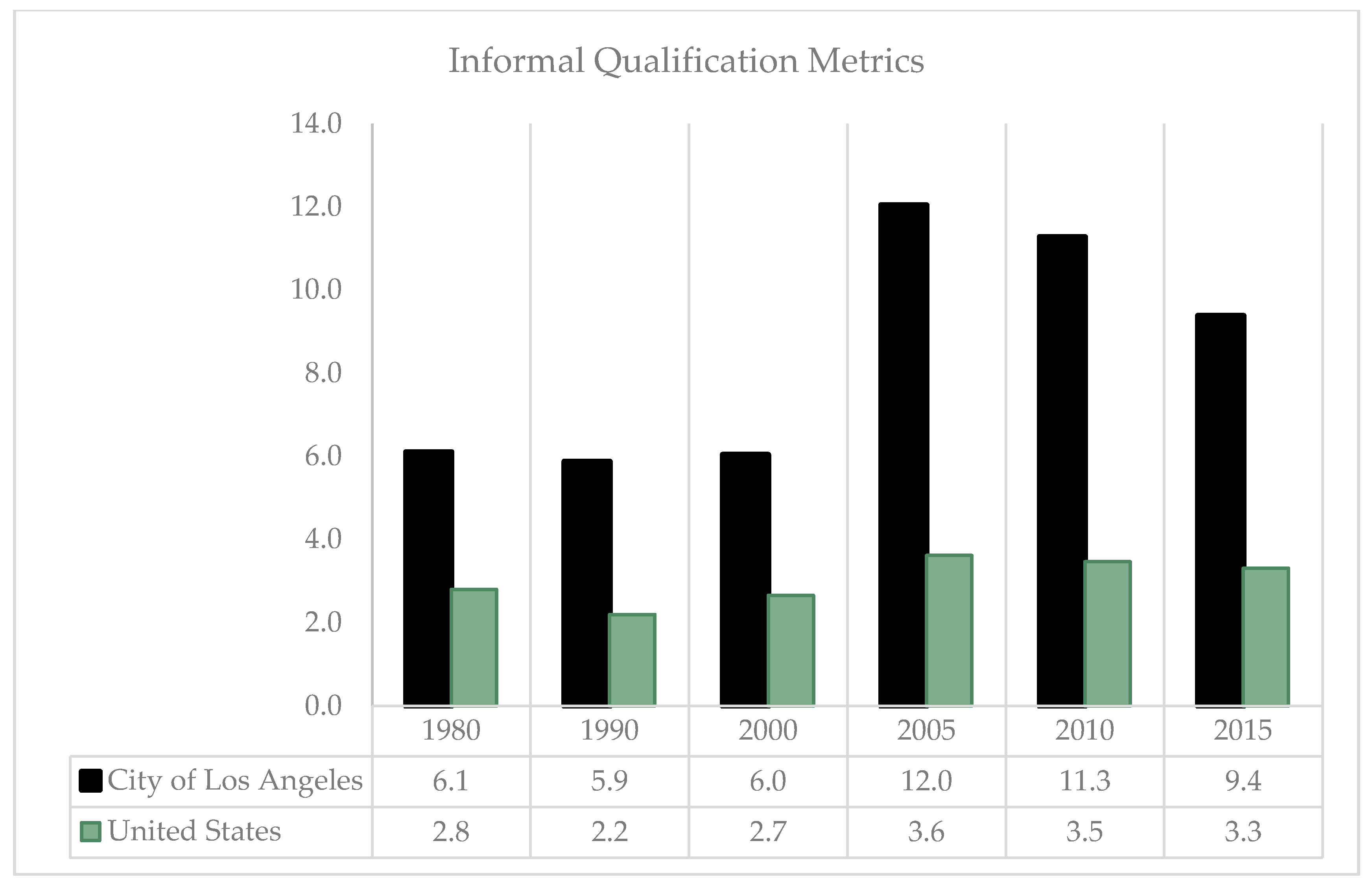
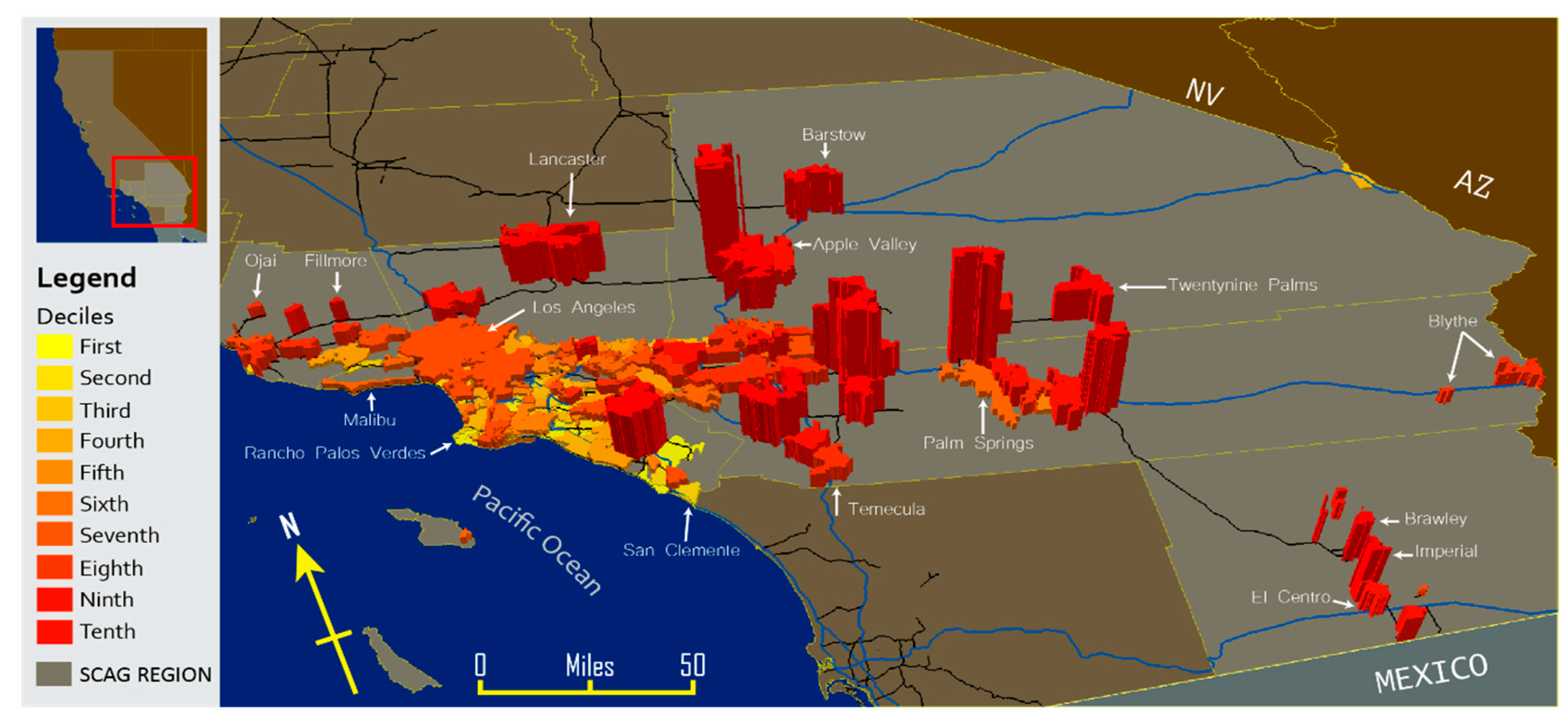
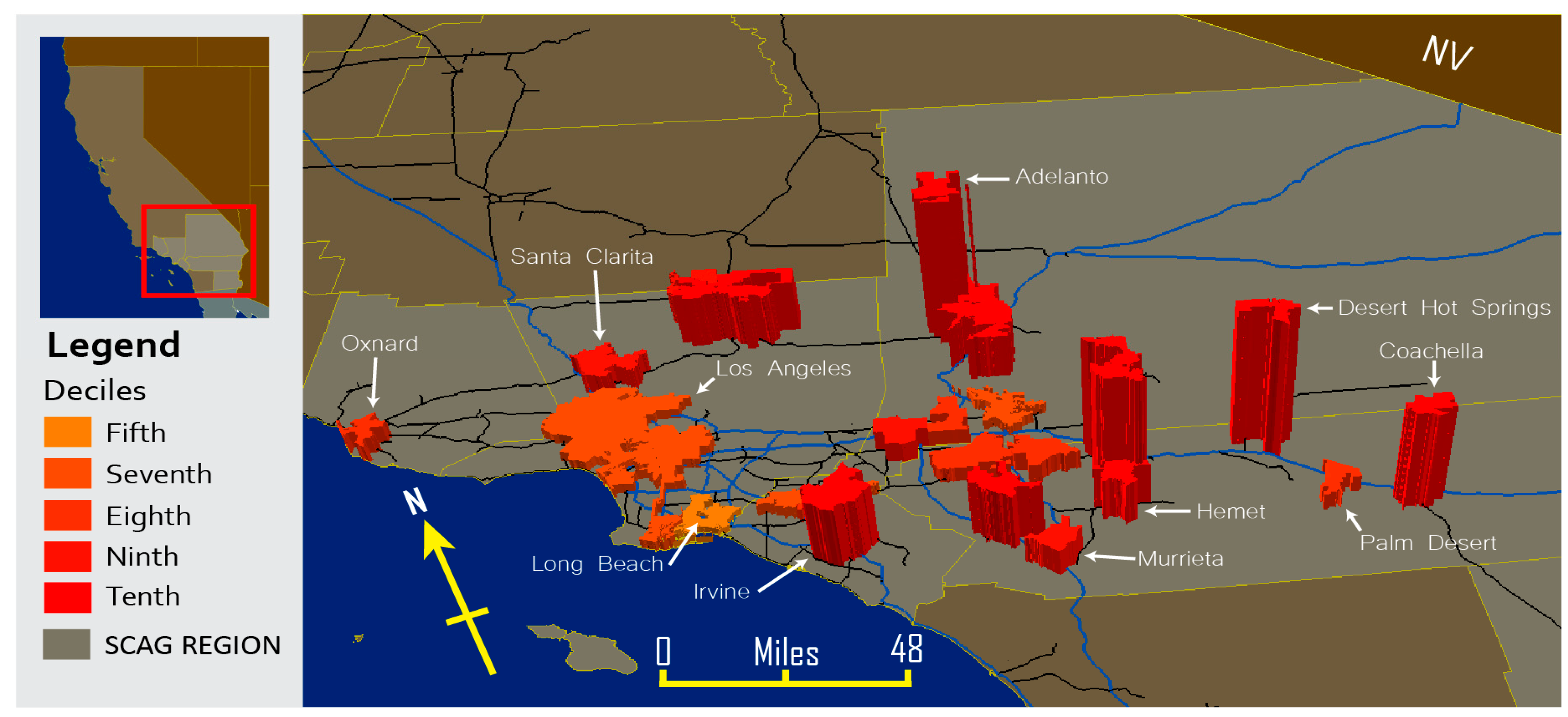
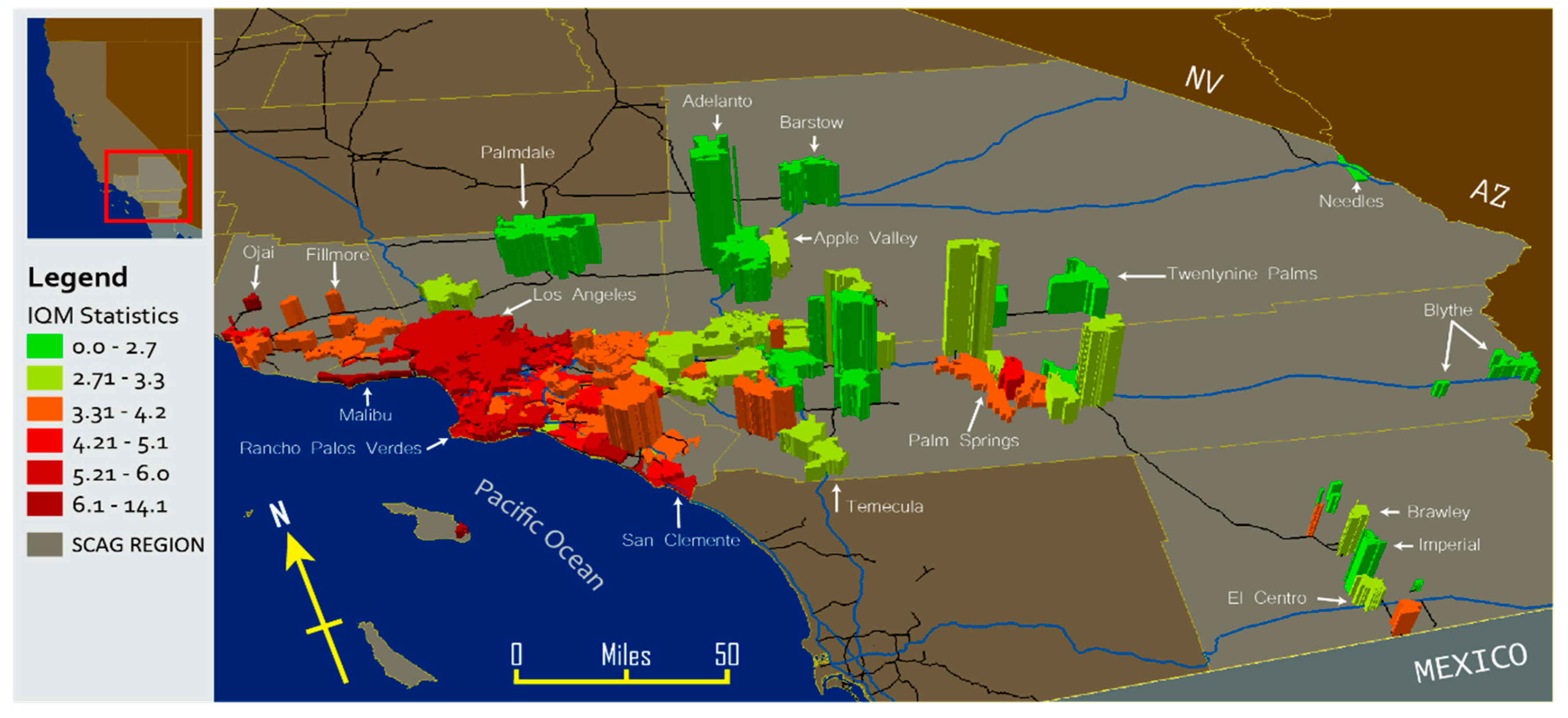
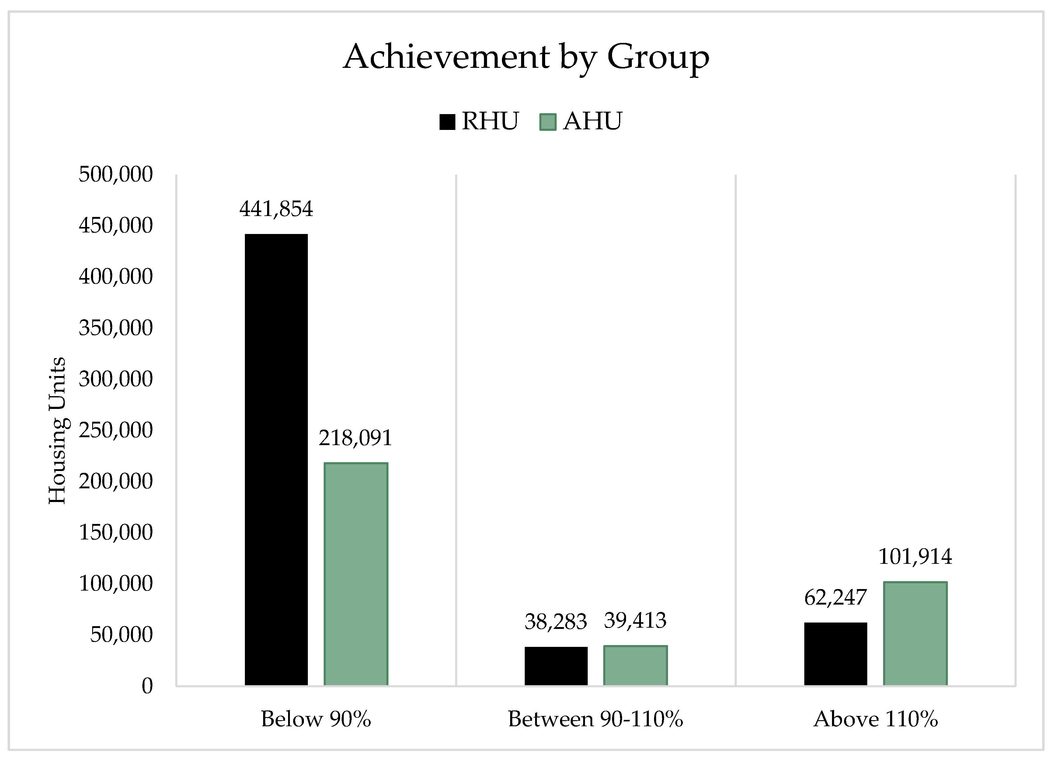
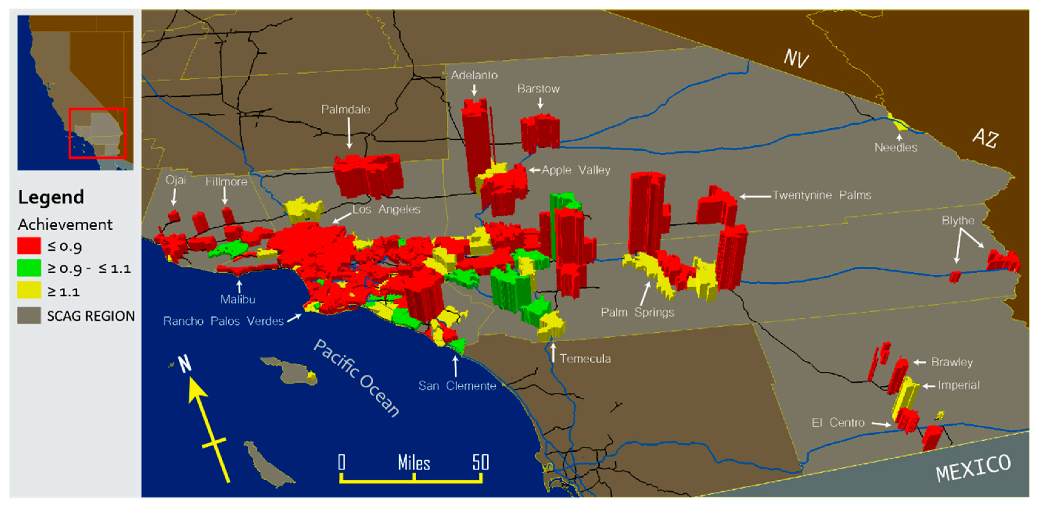
Table 1.
The regional housing needs allocation for the city of Glendora (2006–2014) with the corresponding household income limits. In 2008, HUD determined that the median family income for Los Angeles County was $59,800. The area median income (AMI) for Los Angeles County is calculated as a percentage of HUD’s median family income and includes adjustments for families of different sizes [34]. Sources: [35,36].
| Income Group | RHNA Allocation | Los Angeles County Household Income Limits (FY 2008) Household of 4 Persons |
|---|---|---|
| Very Low (<50% AMI) | 192 | Up to $37,900 per year |
| Low (51–80% AMI) | 119 | Up to $60,650 per year |
| Moderate (81–120% AMI) | 127 | Up to $71,800 per year |
| Above Moderate (121% + AMI) | 307 | Above $71,800 per year |
| Total | 745 |
Table 2.
The Sample’s Descriptive Statistics. Note. RHNA = regional housing needs allocation; IQM = informal qualification metric. Sources: Southern California Association of Governments. California’s Department of Finance, the U.S. Census Bureau.
Table 2.
The Sample’s Descriptive Statistics. Note. RHNA = regional housing needs allocation; IQM = informal qualification metric. Sources: Southern California Association of Governments. California’s Department of Finance, the U.S. Census Bureau.
| RHNA Growth Rate | RHNA Households | IQM 2000 | Housing Inventory 2015 | Actual Growth Rate | Achievement | IQM 2015 | |
|---|---|---|---|---|---|---|---|
| Mean | 12.7% | 2931.8 | 4.2 | 30,684.08 | 7.4% | 92.6% | 6.6 |
| Median | 5.9% | 985.0 | 3.9 | 16,233.00 | 3.3% | 59.0% | 6.3 |
| SD | 19.4% | 8975.6 | 1.5 | 106,652.28 | 12.5% | 236.3% | 2.5 |
| Min | 0.1% | 8.0 | 2.0 | 397 | −5.8% | −1150.0% | 2.3 |
| Max | 119.5% | 112,876.0 | 14.0 | 1,440,779 | 105.9% | 2534.0% | 17.8 |
Table 3.
The Pearson correlation analysis of the sample.
| Pearson Correlation | |||||
|---|---|---|---|---|---|
| Housing Inventory (2015) | IQM (2015) | ACH | AGR | ||
| RHNA Growth Rate (RGR) | −0.026 | −0.457 ** | −0.096 | 0.718 ** | |
| BCa CI 95% | Upper | −0.516 | 0.606 | ||
| Lower | −0.417 | 0.831 | |||
| RHNA Households (RHH) | 0.934 ** | −0.052 | −0.037 | 0.182 * | |
| BCa CI 95% | Lower | 0.495 | 0.062 | ||
| Upper | 0.983 | 0.616 | |||
| N | 185 | 185 | 185 | 185 | |
Notes. * = p < 0.05 level (2-tailed). ** = p < 0.01 level (2-tailed). ACH = achievement. AGR = Actual Growth Rate. BCa = bootstrap results are based on 1000 bootstrap samples. CI = confidence interval. IQM = informal qualification metric. RHNA = regional housing needs allocation. Sources: SCAG, California’s Department of Finance, the U.S. Census Bureau.
© 2020 by the author. Licensee MDPI, Basel, Switzerland. This article is an open access article distributed under the terms and conditions of the Creative Commons Attribution (CC BY) license (http://creativecommons.org/licenses/by/4.0/).
Share and Cite
MDPI and ACS Style
Ramsey-Musolf, D. The Efficacy of Allocating Housing Growth in the Los Angeles Region (2006–2014). Urban Sci. 2020, 4, 43. https://0-doi-org.brum.beds.ac.uk/10.3390/urbansci4030043
AMA Style
Ramsey-Musolf D. The Efficacy of Allocating Housing Growth in the Los Angeles Region (2006–2014). Urban Science. 2020; 4(3):43. https://0-doi-org.brum.beds.ac.uk/10.3390/urbansci4030043
Chicago/Turabian StyleRamsey-Musolf, Darrel. 2020. "The Efficacy of Allocating Housing Growth in the Los Angeles Region (2006–2014)" Urban Science 4, no. 3: 43. https://0-doi-org.brum.beds.ac.uk/10.3390/urbansci4030043