Article

Urban Form, Socio-Demographics, Attitude and Activity Spaces: Using Household-Based Travel Diary Approach to Understand Travel and Activity Space Behaviors

1
Institute of Transportation Science, University of California (Irvine), Irvine, CA 92697, USA
2
Department of Urban Planning and Public Policy, School of Social Ecology, University of California (Irvine), Irvine, CA 92697, USA
*
Author to whom correspondence should be addressed.
Submission received: 1 November 2020 / Revised: 27 November 2020 / Accepted: 30 November 2020 / Published: 2 December 2020

Abstract

:
Very few studies have addressed the gap in literature by examining the travel and activity patterns of travelers in developing countries to inform future land use and socio-economic planning. The major purpose of this paper is to determine the factors related with travel and activity space patterns of residents in Dhaka, Bangladesh. Based on lessons learned from a pilot study, a full study was undertaken using artificial neural network and regression. A network analyst-based shortest path network with road network buffer activity space calculation measure was used in geographic information system. Exploratory and confirmatory factor analyses were used to identify attitudinal factor dimensions. Calculated individual activity spaces were found to range from 0.08 to 10.13 square miles. Trip characteristics were found to be significant predictors of individual activity space. In case of household activity space, D variables (density, design, and destination accessibility) and household characteristics were found as the most significant. Perceived neighborhood amenities, car attachment, monetary concerns, transit preferences, perceived daily travel area and environmental concern were found to shape people’s perception. Weekend activity spaces were more compact than those for weekdays. Individual day-to-day variability was less during weekdays than on the weekend. Female and high-income respondents had smaller activity spaces.

1. Introduction

With an area of only 116.6 square miles, Dhaka Metropolitan Area (DMA) has a population of approximately 12.6 million people which makes Dhaka as one of the most densely populated cities of the world [1]. A few gender-based studies tried to explore the travel/activity situation of Dhaka from spatial planning perspective [2,3,4,5,6,7,8,9] and very few of them focused on spatial/locational distribution of households. However, as per our knowledge this is the first study analyzing the existing travel behavior of the residents of Dhaka based on geographic distribution of household activities through calculating traveler’s activity space. A qualitative research conducted by Islam (1995) aimed to understand the activity patterns and gender relations of middle-income working women in Dhaka in private and public space [5] which found that gender division of labor exists and women’s gender roles in the predominantly patriarchal society create fixity constraints for them which eventually limit their public activity space. This study was one of very few and was almost the first of its kind to explore activity and social pattern of women, gender relations and temporal changes in the activity spaces in Dhaka. Another gender-based study related with spatial planning conducted by Gomes (2014, 2015) showed that upgrading women’s socio-economic status expands their activity space and plays an important role in domestic spatial organization of urban houses in Dhaka [10,11]. In Uddin, Burton, &Khan (2018) specific environmental barriers were found to reduce female physical activity space [8]. None of the previous Dhaka studies assessed activity space variation of travelers with respect to their individual and household characteristics; and attitudes/perceptions and whether they can access essential service facilities within their travel/activity area. In this context, it was important to establish a relationship between accessibility to various urban opportunities with travel and spatial behavior and to depict the variability pattern in the activity spaces of travelers to predict the transport and travel needs of people as accessibility to necessary urban facilities plays important role in shaping travel behavior and activity pattern. In addition, it was important to explore the relationship pattern between activity space and land use, socio-economic, travel characteristics.
A pilot study [12] was undertaken by Sharmeen & Houston (2019) in Dhaka before this full study. The pilot study results suggested the value of collecting more trip-related information in the full survey (see Supplementary Materials) within a travel diary of the respondents; therefore, additional travel characteristics (travel duration, distance, and cost of each trip) were accommodated in this full survey questionnaire. Sample size and data collection time span (number of days in travel log) were expanded in this full study. Different sets of indicators were evaluated in this paper. A thorough literature review was conducted to identify most suitable models, sets of indicators, and measurement techniques. Based on lessons learned from the Dhaka pilot study, the expanded set of objectives for this full study include: (1) conduct descriptive analysis of travel-activity patterns in two study sub-areas (Dhanmondi and Mirpur) and some combined descriptive analysis by weekdays and weekends; (2) analyze the relationship between travel-activity patterns with built form, socio-economic, travel, and attitudinal characteristics; (3) establish a relationship between accessibility to various urban opportunities with travel and spatial behavior by sub-area; (4) examine intrapersonal and interpersonal variability of household’s activity spaces. Major purpose of the paper is to determine the factors related with travel and the activity space patterns of residents in one of the densest cities of the developing world and to test whether the size of the observed activity spaces is associated with land use, socio-demographics, travel characteristics, and perceptions. This study is expected to respond to a gap in the literature by examining the travel and activity patterns of travelers in Dhaka City to inform future land use and socio-economic planning. Significant factors that affect the spatial distribution of activity locations were explored here and results from the analysis are expected to be used to reflect on transportation policy guidelines. This article is structured as follows: the next section reviews research on activity space calculation methods and the factors determining their sizes and is followed by a description of the research setting, data sources and analytical methods. This is then followed by an outline of the results, using descriptive statistics, artificial neural networks, regression modeling, accessibility, and variability analysis. The paper ends with some discussions and proposals for future research.

2. Literature Review

Several techniques were employed in numerous studies to calculate activity space and to measure the impact of urban form, socio-demographics, and personal attitudes on human activity spaces and travel pattern. A general linear model (GLM) was used to determine weekly activity location in Järv, Ahas, & Witlox (2014) [13]. To measure the residential density (land use mix/diversity analysis, road connectivity analysis), logistic regression was used [14]. It was used to examine the influence of the proportion of different land uses on different variables measuring physical activity (walking etc.). Multi-level regression was used in Lee et al., 2016 [15]. Regression model was used in Tana, Kwan, & Chai (2016) [16] while hierarchical multiple regression and correlation analysis were used by Vich and Miralles-guasch (2017) [17]. Guerra et al., 2018 used Logit and OLS models to identify the impact of population density, land use diversity, intersection density, accessibility measures, socio-economic factors, and car ownership status [18]. Correlation analysis was conducted between age and gender with radius, shape, entropy of activity space [19].
According to Handy, Boarnet, Ewing, & Killingsworth (2002); common measures of the built environment include land use type, density (e.g., residential density), land use mix and street connectivity (e.g., intersections per km2) [20]. While defining unique areas, some activity space-based studies used locational information (e.g., addresses, postal codes). The most common method to calculate activity space has been to establish a circular buffer around a respondent’s geocoded location at a given radius [21,22,23,24]. A shortcoming is that a circle may not accurately represent the spatial area. Circular buffers are likely to be inaccurate in areas with natural or built features with poor street connectivity. In such cases, areas within the buffer may be inaccessible by the respondent but still used to calculate built environment measures. This method includes all land up to a certain distance from the individual and fails to account for how the existing road network restricts the way an individual can traverse the landscape. The other buffer approaches (polygon-based and line-based network buffer) consider how the road network restricts travel, affecting what is accessible within travel. The polygon-based network buffer uses the end points of certain journeys in the network as the vertices with which to construct an irregular polygon to define the accessible neighborhood. The method presented in Oliver, Schuurman, & Hall (2007), defined the 1 km neighborhood by applying a 50 m buffer to a 950 m line-based network buffer, thus more closely approximating the roads accessible to the individual [14].
Schönfelder (2006) defined variability as the deviation of behavior from the usual individual routines and habits which were developed over longer time periods. Inter-personal variability is the deviation of the individual behavior from the mean behavior of the respective sample or of the socio-economic group the traveler belongs to. The behavior of an individual or a household varies considerably if they are observed over periods of time which exceed a pre-defined timespan such as one day. This kind of variability is called intra-personal variability [25].
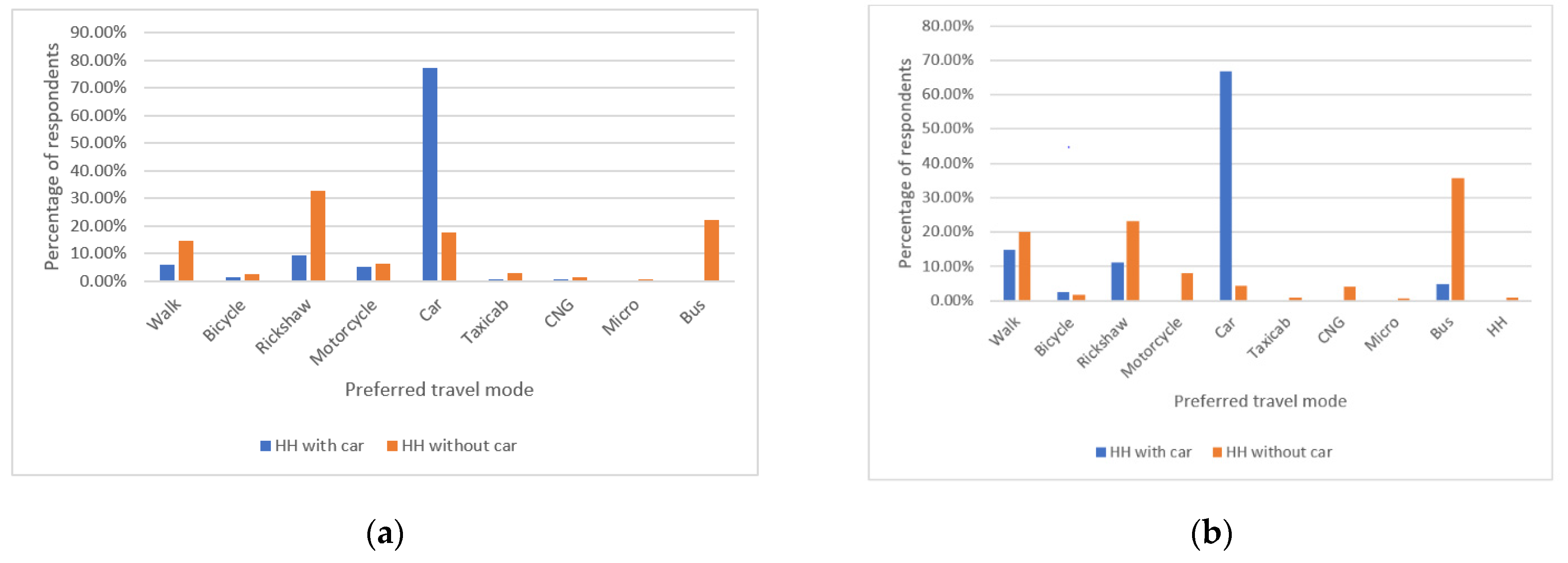
Dieleman, Dijst, & Burghouwt (2002) in their study found that apart from urban form and design, personal attributes and circumstances have an impact on modal choice and distances travelled [26]. High income people are more likely to own and use a private car than low-income households which is also a common scenario in Dhaka. Another finding of this study was that families with children use cars more often than one-person households. Trip purpose also found to influence travel mode and distance. Hägerstrand (1970), in his pioneering work titled “What about People in Regional Science?”, mentioned about fixity constraints focusing on the issue that despite being in spatial proximity to any given location, a person cannot travel to it due to some other mandatory works in the given period [27]. This relates to the spatial-temporal aspect in an individual’s activity space. In recent times, Mei-Po Kwan (2003; 1998; 1999a; 1999b; 2000; 2002) demonstrated different space-time models to show disparities in gender accessibility within the same household [28,29,30,31,32,33].

3. Materials and Methods

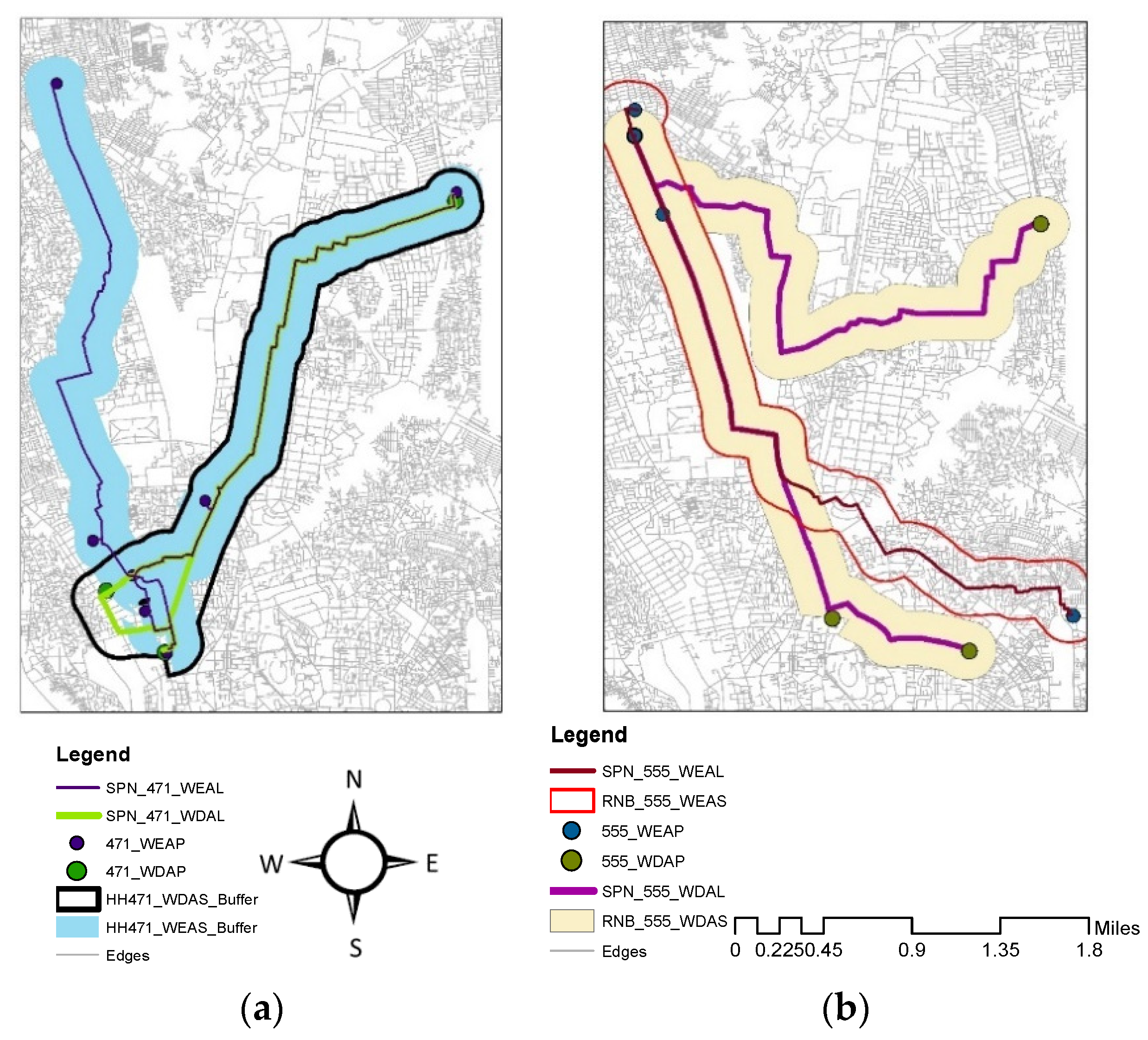
Calculation of household activity space [34,35] and person-wise analysis by measuring individual activity space both were conducted in this paper. For calculating household activity space, locations were geocoded through creating two types of shapefiles in ArcGIS 10.7.1. Weekday shapefile per household (HH) defines one location shapefile containing all member’s travel location points from a specific HH for five consecutive weekdays (day 1–5: for Dhaka weekdays are from Sunday to Thursday). Weekend shapefile per HH defines another location shapefile containing all member’s travel location points from a specific HH for two consecutive weekend days (day 6–7: Friday and Saturday). Thus, each sample HH has at least three or more activity locations and visited at least two non-home places. With these, intrahousehold variability of activity spaces between weekday and weekend were assessed/examined following Dharmowijoyo, Susilo, & Karlstrom(2016); Dharmowijoyo, Susilo, & Karlström (2014) [36,37]. Regarding the construction of activity spaces for weekdays and weekend, all declared destinations for 5 weekdays and 2 weekend days were combined, respectively, but frequency of visiting each destination (for example: 5 times vs. 1 time per week) were not considered.
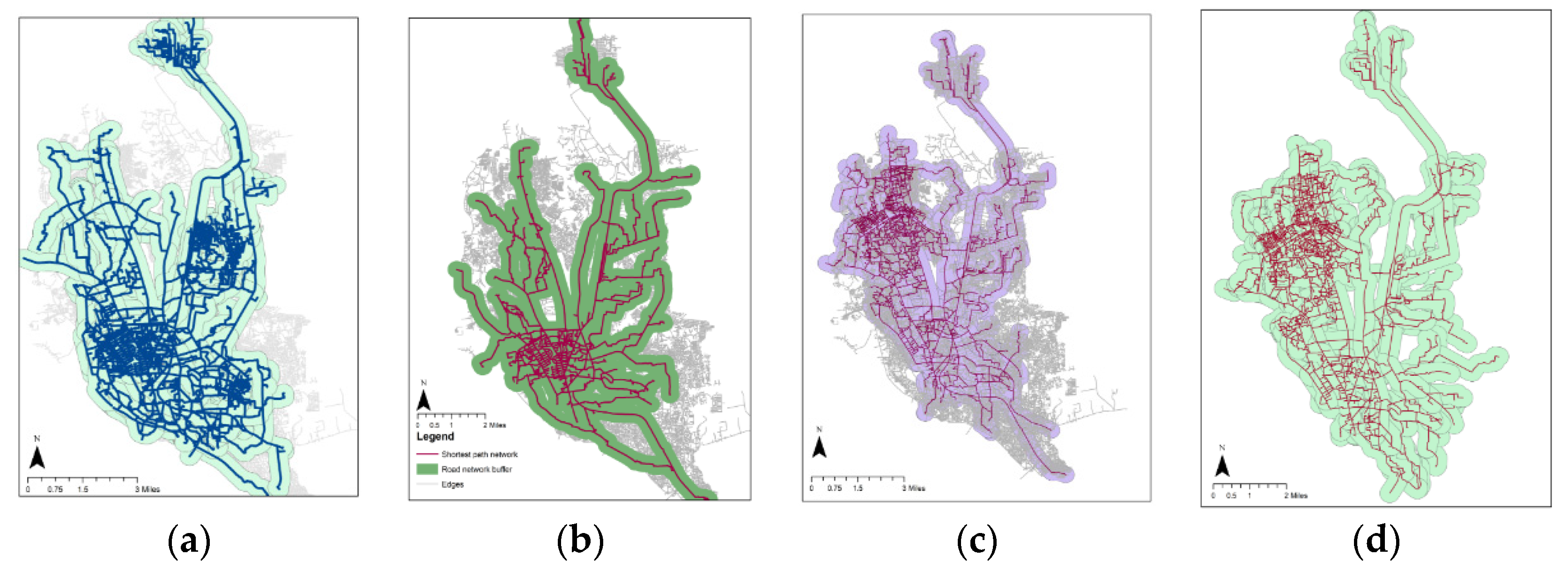
In this paper, to calculate activity length and area (activity space), ArcGIS-based activity space measure of shortest path network with Road network buffer measure was used as land use characteristics generally show greater associations with walking using line-based road network buffers rather than circular buffers. The selection of network or circular buffers has a considerable influence on the results of analysis. Careful consideration of the most appropriate buffer with which to calculate land use characteristics is important: 0.5 and 1 mile network buffer (residential network buffers covered by activity spaces stratified by sociodemographic characteristics); 1 km circular and line based road network buffer (RNB) (polygon-based network buffer, buffered line-based network buffer: 50 m buffer to a 950 m line-based network buffer resulting in a 1000 m buffer); 200 m buffer daily path area was used in the previous literature to calculate activity space [14,15,38]. In this paper, a 0.25-mile (400 m) road network buffer was used considering a previous study finding [39] on average trip length of walk mode (15 min) in Dhaka Metropolitan. Therefore, a 400 m buffer was chosen based on the average travel distance covered in a 5 min walk trip (assuming 5 min as a comfortable walking distance for all age groups of travelers), to ensure that parcels along the roads would be included but that most parcels located further from the road (e.g., behind those adjacent to the road) would not be selected. This method is based on the idea that land use encountered along roads is most important in characterizing a neighborhood in the way it is experienced by residents walking through it, and land not accessible to the pedestrian, even if physically nearby, is not part of their 400 m walking neighborhood. In this paper home-based activity space [40] was calculated. ArcGIS network analyst was used to calculate the 400 m shortest path network-based buffer along the road network from each respondent’s postal code centroid (home location) to the destinations visited. Only the portion of parcels that were within 400 m of the roadway were included in calculations. This may represent a better approximation of potential destinations locally accessible to the individual respondent.
Descriptive analysis of the variables with comparison of activity spaces across the two study sub-areas were conducted as per the first objective. Second objective of the paper was to analyze the effects of residential location characteristics (urban form), socio-demographics, attitudes, and trip characteristics on the resulting average activity spaces. D variables (development density, intersection density, accessibility to various service facilities / destination accessibility) were selected to quantify land use characteristics following Park, Ewing, Sabouri, & Larsen (2019) [41]. Most of the studies of travel and activity pattern employed different regression analysis due to the method’s ability of incorporating numerous variables [13,14,15,16,17,18,21,36,42]. The regression equation can be presented in many ways, for example:
Ypredicted = β0 + β1 × X1 + β2 × X2 + ………… +βn × Xn
where Yi refers to the dependent variable, Xi (X1…. Xn) refer to the independent variables, β0 is a constant and β1…. Βn are the coefficients to be estimated. Multiple linear regression was employed as the preliminary analytical method to investigate the potential impacts in this paper. We examined both weekday and weekend travel in separate models since previous research indicates weekday travel-activity patterns can significantly differ from weekend patterns [13]. We examined individual and household differences on the size of activity spaces using regression model to assess the relative influence of household, socio-demographic, and accessibility factors on these measures of spatial behavior for both weekday and weekend trips. Our model assumption is that the dependent variable is a linear function of the independent variables and takes the following form:
AS = f (HH, SD, TP, ASF, UF, PP)
where f() is a linear function; AS is an activity space measure (RNBAREA: road network buffer area and SPNLENGTH: shortest path network length), HH is a vector of household factors including presence of children, household size, employed persons, presence of elderly persons, car ownership status and household vehicles, number of cars used; SD is a vector of socio-demographic factors for age, gender, employment status, occupation, income, marital status, educational level, population density. TP includes individual travel pattern indicated through use of carpool, work from home or not, public transit use, average number of trips, trip duration, cost, distance traveled. ASF denotes accessibility to various service facilities (job, shop, school etc.) and UF indicates land use characteristic (intersection density). Lastly, PP indicates people’s perception derived from exploratory and confirmatory factor analysis of 36 Likert scale statements.
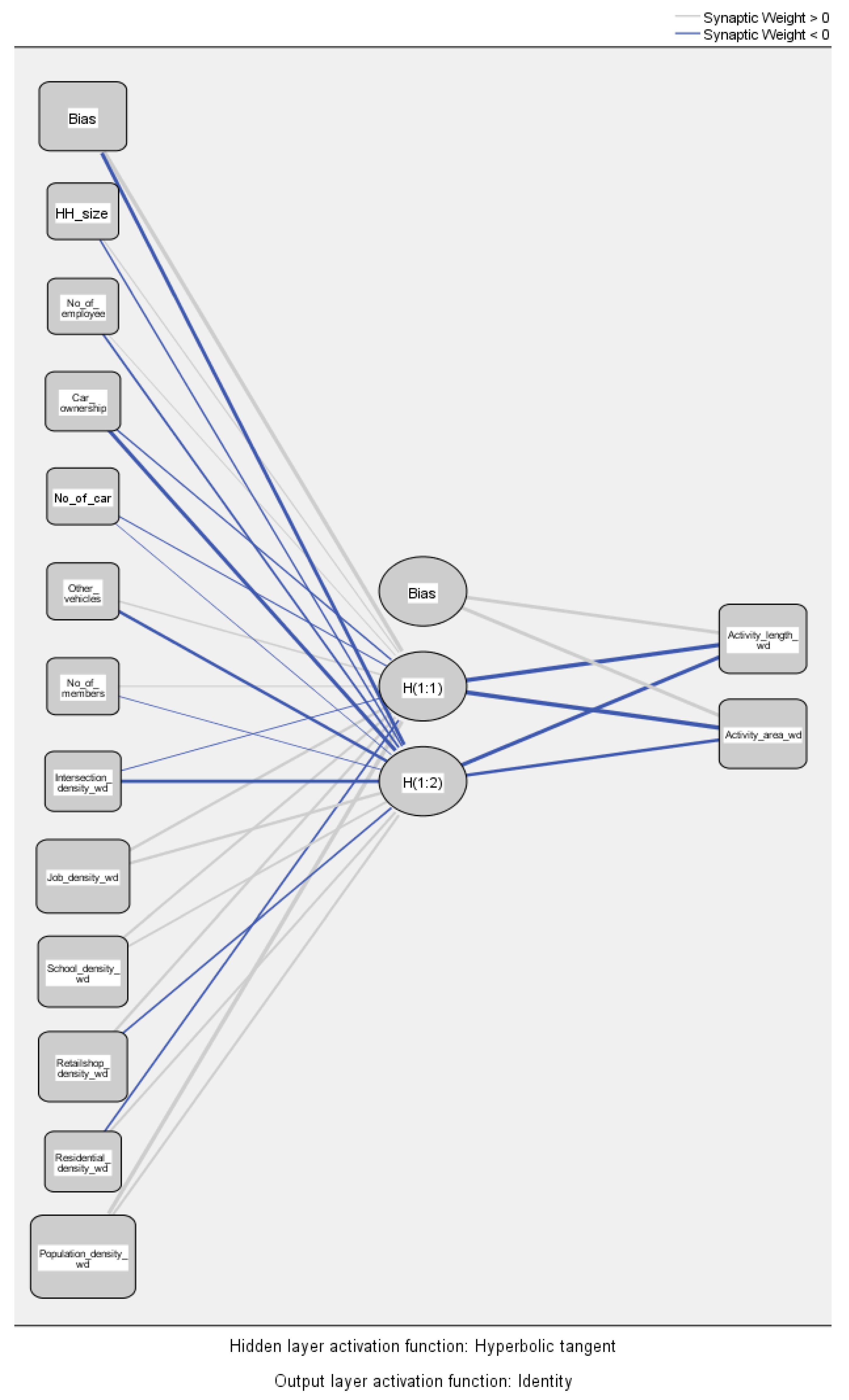
Another model we have used in this paper is the artificial neural networks (ANN) model which is an alternative to the multiple regression analysis to better explain the dependent variable (activity space). This analytical approach can overcome some limitations of the other model stated. It can handle nominal, ordinal, and scale variables either as dependent or independent and can handle nonlinearity relatively easily without knowing beforehand exactly which type of nonlinearity exists. This can solve highly nonlinear problems; the mixture of data types can be as input into the ANN, making no assumptions regarding the distribution of the data, and can use many variables or factors, some of which may be redundant [43]. According to Maithani, Jain, & Arora (2007), ANN based modeling fits into the category of regression-type model, the aim of which is to establish a functional relationship between a set of spatial predictor variables that are used to predict the locations of the change in urban landscape [44]. This is a non-parametric technique for quantifying and modeling complex travel behavior and patterns. Among the 7 types of artificial neural networks available for analyzing data, multilayer perceptron (MLP) was used in this paper. The MLP consists of three types of layers, i.e., input, hidden and output layers. The ANN is described by a sequence of numbers indicating the number of neurons in each layer.
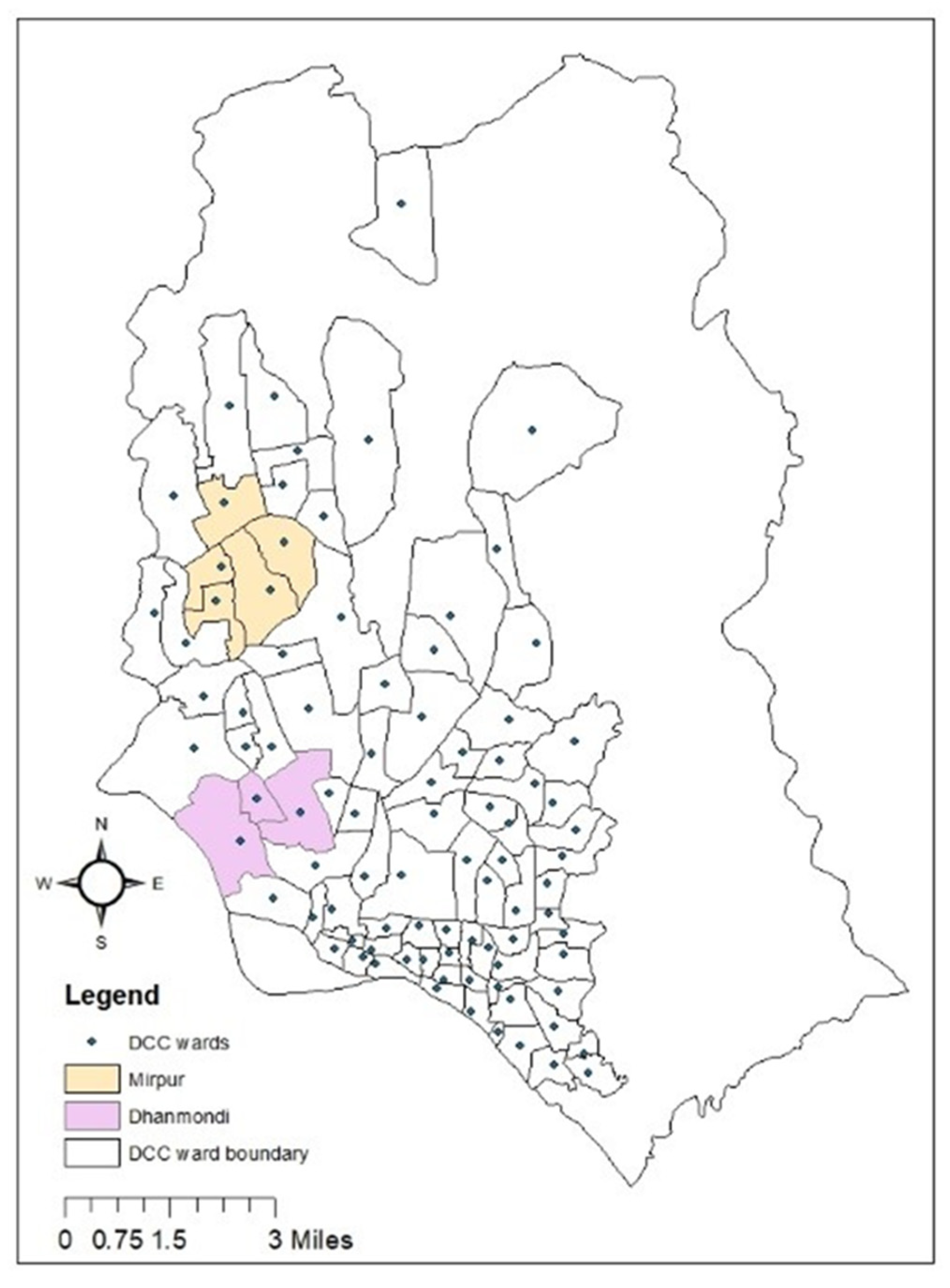
This study focused on two separate sub-areas: Mirpur from Dhaka North City Corporation and Dhanmondi from Dhaka South City Corporation based on their distinctive socio-economic and transportation characteristics. The majority of Mirpur is an unplanned residential area; building and road networks here follow no specific pattern and in most of the cases, residential buildings violate the setback and floor-area ratio (FAR) rules of city building regulations. On the other hand, in Dhanmondi, residential areas are mixed with commercial areas. Lots of mixed-use buildings are there. Planned residential area with grid iron pattern road network is the main feature in Dhanmondi. Profile of the two study sub-areas (description of the case city, why these neighborhoods were represented, how they are similar/different), survey design and primary data collection procedure (what households were contacted, sampling method, how was the survey carried out) were discussed in detail within our pilot data analysis-based paper [12] which was also published in Urban Science. Two study sub-areas in Dhaka are shown in Figure 1.
Overall, 1000 households and 1790 travel logs from these households were taken as study sample. As numbers of surveyors were few so, the total survey period was quite long. Although the weeks surveyed vary across households, it was tried to ensure that the results could not be affected by characteristics of surveyed weeks, for instance dry/wet seasons. Accordingly, we attempted to select a normal week to survey each of the households. In the travel log (trip diary), provided to each member from the selected households aged greater than 10 years (if children under this age mostly visit with other adult family members), they were asked about the specific address of their destinations. Parcel data instead of precise xy coordinates for activity locations were used while geocoding in ArcGIS. Institutional Review Board (IRB) approval was needed before any primary data collection for research and IRB approval was taken from University of California, Irvine (UCI), whereas, as an exempt category of research, no such kind of approval is necessary in Bangladesh for primary data collection. Any non-household member who presented in the household during survey time did not fill out surveys. Confidentiality was maintained for collecting female travel logs. One precondition of IRB approval was to make sure people feel protected and can provide their answers especially in case of female respondents without a male controlling them. Mostly one family from each housing unit was surveyed in case of housing units with multiple families. Address list from the municipalities were obtained and every 10th household from that list was contacted. Study sample was stratified within the population as per sub areas. So, it can be said that stratified random sampling method was followed in case of recruiting households. A “normal week” with weekend was studied for each household as the distributions of activities over the weekends are also important. All members from the selected households who traveled outside during the respective selected survey weeks (keeping the home location as the origin of the first trip of each day) filled out the logs. Each trip along with all trip segments respondents take during each day of the week was considered. The route taken was not declared. While calculating activity area, the shortest path was assumed as the actual path taken. Multiple plausible routes were not tested which is a limitation of this method. In case of secondary databases, road network data and land use dataset sources were Local Government Engineering Department (LGED), Capital development authority RAJUK, 2016; and Dhaka Structure Plan 2016-35 [45]. Previously for pilot data analysis [12], the 2010 dataset was used but for this paper, the most recent available datasets were used.

4. Results

4.1. Comparative Analysis between Two Study Sub-Areas

In Dhanmondi, car ownership was found to be higher than Mirpur. In Dhanmondi, 18.4% of the sample owned another vehicle (bicycle/motorcycle/CNG/rickshaw) other than a car and about 47.5% owned a car. While in the case of car ownership, Mirpur is lagging far behind (only 16%), in the case of another vehicle ownership, it is almost like Dhanmondi. Independent sample T-tests were conducted for a set of indicators (household size, number of employees, number of cars, number of children and elder persons, distance traveled, travel cost, trip duration) to compare both areas in Table 1. All these indicator’s mean values were found to be significantly different between the two areas except number of elderlies, and distance traveled.
Human travel behavior varies with automobile ownership. A comparative scenario of both study sub-areas is portrayed here in Figure 2. For obvious reasons, households with car ownership had higher level of preference towards the use of cars in both the areas. On the other hand, households which did not own an automobile showed a higher level of preference for rickshaw in Dhanmondi and in Mirpur, respondents’ preferred travel mode was found to be bus. Rickshaw is a non-motorized three-wheeled vehicle, mainly used to travel short distances. This behavior can be explained by the higher modal share of bus (39%) in Mirpur and rickshaw (17.2%) in Dhanmondi and comparatively higher average travel cost found (Table 1) in Dhanmondi. Since Dhanmondi was developed with the characteristics of a planned residential area with traditional grid pattern roads (and collector or access roads), there is a greater potential for short distance trips within the area, which is more readily supported by rickshaws. Given the demographic differences between the two selected study sub-areas, these travel behavioral differences are not surprising, and contribute to the transportation literature.

4.2. Comparative Analysis between Weekdays and Weekend by Two Study Sub-Areas

On an average, Dhanmondi households were found to have larger activity length and space in comparison to Mirpur during weekdays but opposite during weekends. Huge differences between weekday and weekend activity area were found in Dhanmondi but in Mirpur not much variation was observed (Table 2).
In Figure 3, individual activity areas ranged from 0.08 to 10.13 square miles. While calculating travel distance and trip duration, similar findings for activity area and length were observed for both study sub-areas in comparing between weekdays and weekends (Figure 4).

4.3. Combined Analysis of Both Areas

Comparative analysis between weekdays and weekends was done for both areas in a combined manner. To explore the relationship between people’s perception and actual behavior, a gender-based analysis was conducted (Figure 5). While comparing between perception regarding travel mode and actual practice, it was found that actual use of all other modes (specially bus and car use) except walking matched with both male and female preference. In the case of walking, a considerable percentage of both male and female respondents expressed their urge to walk but, less than 5% walk to work. Use of rickshaw also experienced a decline in comparison to the perception or preference towards this mode. So, overall, it can be said that respondents normally expressed preference towards sustainable travel modes (walking, rickshaw) during the survey but in a real scenario, they chose travel modes with respect to comfort and availability. For example, in the Dhaka context, if somebody has accessibility to private automobile, he/she will be very much unlikely to switch to alternative travel modes. Dhaka’s unplanned traffic infrastructure promoting car use can be one of the main reasons for this travel behavior.
In Figure 6 and Figure 7, activity-travel pattern visualizations for all seven days (day wise percentage of trips by trip purpose and modal share analysis) were created to analyze the variation of trip purposes and travel modes. The percentage share of trips by purpose for all seven days was mostly similar among weekdays (day 1 to 5) and between two weekend days; day 6 and 7 (Figure 6). Work trips comprise a significant share of all trips as previously mentioned. School trips are also another major trip type for Dhaka. Return trips to home were found to represent the most common purpose for all trips (these trips were geocoded under trip purpose: home) and travelers normally use the same route or area to return. Days 1–7 are the same days of week for all participants (i.e., day 1 is Sunday and day 7 is Saturday for all).
Home was already denoted as the origin of the first trip (first activity location in most cases) so in activity space analysis, the return trip to home was not considered. Home as trip purpose dominates among all trip purposes for all seven days except one (day 3) as most respondents start daily trip from home and return to home after visiting different activity locations (see Figure 6). Work is the second most dominant trip purpose which was found to secure the highest position on day 3. School is another prominent trip purpose for the travelers from both study sub-areas. Large share of school trips is mainly due to the reason that adult members of the household normally accompany the child to school every day. A higher share of shopping and social contact trips is observed in day 6 and 7 which are weekend days. Work trip shows lowest daily share on day 6 as this day is Friday which is the general weekly religious holiday in Bangladesh.
In Figure 7, car and bus as travel modes dominate the modal share for all seven days of the survey week, indicating both private automobile and public transit dependency of people of the study areas (Dhanmondi is more car dependent and Mirpur is predominantly transit dependent). Among the seven days, car dominates only one single day while bus dominates in modal share for the rest of the days. A significant percentage of respondents use rickshaws; for one single day in the week, the share of rickshaw rides was found as the highest modal share. After these three modes, walking contributes significantly to daily travel. Bicycle, human hauler, taxi, and jeep make up a very limited share of travel modes.
Quantification of attitudinal responses will be done in the next section (Section 4.4: Factor Analysis) of this paper to use in the model. From survey responses, importance of protecting the environment (7.0 out of 7.0) came out as the dominant attitude. Lack of comfort in transit (6.98) was next in importance, followed by easy accessibility to service facilities within daily activity space (6.97). Importance of car (3.35) and car as a symbol of social status (3.8) came out as the least important attributes. The following attitudes were ranked as least important: less use of car to protect the environment; feeling of restriction, deprivation, and social exclusion for not having a car. One of the least important attitudes found (less use of car to protect the environment) is somewhat like the most dominant attitude found which is protecting the environment.

4.4. Factor Analysis

Factor analysis is needed to convert the attitudinal question statements into a smaller set of factors so that those can be included as independent variables in transportation models. To conduct a factor analysis in most studies [46,47,48,49,50,51], the main respondent in each household was asked to rank some attitude- or perception-related statements on a seven-point Likert scale ranging from 1 (strongly disagree) to 7 (strongly agree). The first step in analyzing participant responses to attitudinal questions was to use exploratory factor analysis to reduce the large number of questions to a smaller set of factors for regression analysis. Then, principal component analysis was used as the extraction method with varimax rotation for most of the studies. Based on a scree plot showing the variance explained by each factor, a fixed number of factors were chosen for analysis in most of the cases. Then, Cronbach’s alpha was calculated for each factor to assess reliability and to evaluate the internal consistency of the factors.
From Table 3, it was found that almost 85.6% of the variability can be explained by underlying factors indicating better sampling adequacy. After applying principal axis factoring as an extraction method with the help of rotated eigenvalues in total variance explained and scree plots, 10 factors were found from 36 attitudinal questions. The factors were arranged in descending order based on the most explained variance. Respondents were asked to indicate their preferences on a seven-point ordinal scale ranging from “Strongly disagree” to “Strongly agree” regarding variables. These 36 variables were then factor analyzed in SPSS17.0. Statements were grouped under 10 factors to be added in the regression model. In each factor analysis, the number of factors was determined based on the interpretability of the factors, combined with interpretation of the scree plot and all eigenvalues larger than one. A pattern matrix was built indicating which statements are most strongly associated with each factor. The extraction method using principal component analysis and the rotation method including Varimax with Kaiser Normalization were used. Rotation was converged in 16 iterations. Only factor loadings higher than 0.200 (in magnitude) were reported. Loadings higher than 0.300 characterize the factors to a large extent and they enrich the interpretation of certain factors.
To evaluate the internal consistency of the factors, Cronbach’s alpha was calculated for each. All the factors have Cronbach’s alpha of 0.7 or higher, while the recommended minimum is 0.60 in case of exploratory research [52]. In case of combined reliability statistics, Cronbach’s alpha values were found as 0.768 and 0.831 (standardized) according to which it can be said that Cronbach’s alpha values show sufficient internal reliability in this paper.

4.5. GIS Applications of Methods for Representing Activity Space

Quantification and mapping of activity space will be done in this section. The shortest path network (SPN) and road network buffer (RNB) were applied on the travel log data collected through the Dhaka travel survey. Due to the limited number of daily trips found from the Dhaka full survey, we calculated weekday household activity area comprising all locations visited during five consecutive weekdays by all household members and weekend household activity area comprising all locations visited during two consecutive weekend days by all household members. Even though both types of activity space contain different number of days, some weekday-to-weekend intrahousehold and intrapersonal variability in activity space will be explored in Section 4.9: Variability of Activity Spaces. Though not every household was of same size (equal number of members), inter household activity space variability can be analyzed as Dhaka travel log comprised all travels conducted by the selected household members in the selected survey weeks. Travel information of any selected household members which was not included in the travel log did not travel outside in the respective survey weeks. These individuals are mainly non adult (children), elderly people and in some cases unemployed females (homemakers) and some members working from home. Later, individual weekday and weekend activity space was calculated for a sample size of 1000 (by taking one individual from each household). Individual activity space also takes part in further analysis for this paper. The reason for not calculating the daily activity space in this paper is mainly because some initial analysis for capturing day-to-day variation in activity space showed repetitive daily activity locations visited along the five weekdays.
The shortest path network complemented with road network buffer method was used to calculate activity space, as this method does not overestimate the spatial area traveled by the respondents. The SPN and RNB methods are useful for investigating the accessibility to potential services/opportunities, which will be explored later in this paper in Section 4.8: Household Accessibility Using Activity Space. The sample shortest path networks with 400 m road network buffer for one individual respondent from both study sub-areas are shown in Figure 8.
It can be noticed here that for Dhanmondi respondent (Figure 8a) weekday activity space is smaller in comparison to the weekend which is a little bit unusual as in Dhaka people travel more during weekdays in comparison to weekends (mandatory activities are mostly undertaken rather than discretionary activities which was one of the initial hypothesis of this study). Mirpur respondents’ weekday activity space was calculated as bigger than the weekend activity area (Figure 8b). The road network buffer for both areas in both weekdays and weekend days with the separate-path network is shown in Figure 9, which depicts the buffer (RNB) with transparency, so that the SPN travel paths around which the RNB are based is visible. Although several maps are produced using GIS, due to the overlapping buffer areas among the respondents, the resultant outputs are not that much clearer with maps.

4.6. Quantification and Mapping of Built Form Indicators

Quantitative measures of built form indicators were selected in this paper according to data availability and applicability (Table 4).
In terms of road connectivity, the activity space of respondents from Mirpur was found to have relatively better connectivity in comparison to Dhanmondi (Figure 10). While calculating activity space, weekdays cover all the trips along five consecutive weekdays and weekends cover all trips along two consecutive weekend days of the survey week (capturing the scenario of all 7 days).

4.7. Model Development

4.7.1. Multiple Regression Analysis

Multiple regression was carried out after dummy coding variable as multiple regression cannot handle a nominal variable with more than two levels. For this reason, some independent variables were recoded as dummy variable. Some other variables were taken as reference variables to compare with and were excluded from the analysis. First, multicollinearity was checked among the predictor (independent) variables used in Model 1 and 2. There was no collinearity issue between any of the pairs of independent variables except between two pairs of variables which were (a) use of carpool to work and work from home and (b) employment status: not employed and occupation: unemployed (this pair was expected to be correlated). For these pairs, stronger Pearson correlation values of 0.735 and 0.859 arose.
(1)
Model 1: Individual Weekday Model
Collinearity diagnostics (Tolerance < 0.1; Variance Inflation Factor (VIF) > 10 and Tolerance < 0.2; VIF > 5) were checked. Here, for employment status: not employed and occupation: unemployed, VIF values were greater than 5. So, there was an issue of multicollinearity between these two independent variables, one of the variables (employment status: not employed with higher VIF) was dropped from the model. Adjusted R square 0.236 tells us that 23.6% of the variance in dependent variable is explained by the independent variables (Table 5). From ANOVA table (Table 6), we have statistically significant findings (p-value < 0.05). Overall, the regression model is significant while taking this study’s set of predictor variables as a group; they predict the dependent variable activity space significantly.
From coefficient values, it was found that age category dummy (18–20 years), income level dummy (less than USD 177), average daily distance traveled and average daily trip duration during weekdays have a statistically significant impact on outcome variable of this model: individual weekday activity space with p-value < 0.05. From unstandardized coefficients, it can be said that gender (female), unemployed and retired respondents with respect to students; age category (18–20) and (25–34) years with respect to middle age group (35–54), high income group (income greater than 887 USD) with respect to middle income group (356–592 USD), education level: primary (less than standard class five) and Higher Secondary Certificate (HSC) which is mainly equivalent to community college degree with respect to graduate, unmarried with respect to married people, average daily distance traveled during weekdays and seven perception-related factors are negatively associated with individual weekday activity space. The more these individual characteristics are observed within a respondent, the smaller their activity spaces are. With the increase in all other variable units, individual activity space increases during weekdays.
(2)
Model 2: Individual Weekend Model
While checking the collinearity diagnostics for employment status: not employed and occupation: unemployed, VIF values were greater than five. So, there was an issue of multicollinearity between these two independent variables, one of the variables (employment status: not employed with higher VIF) was dropped from the model. The adjusted R square 0.295 means that 29.5% of the variance in the dependent variable is explained by the independent variables (Table 7). From the ANOVA table (Table 8), we have statistically significant findings (p-value < 0.05). It can be said that the regression model is significant as we have an R2 significantly greater than zero.
From coefficient values, it was found that the variables public transit use, income level dummy (USD 177–355), average daily trip duration and average daily travel cost during weekdays have a significant impact on the outcome variable of this model (p-value < 0.05): individual weekend activity space. Among the 10 perception-related factors, five factors have significant impact. From unstandardized coefficients, it can be said that work from home, three perception-related factors, gender (female), unemployed, govt. service and retired respondents with respect to students; aged people from the category greater than 65 years old with respect to the middle age group (35–54), low (less than USD 177) and high income groups (income greater than USD 887) with respect to the middle income group (BDT 356–592), education level: primary, highly educated with respect to graduates and unmarried with respect to married people are negatively associated with individual weekend activity space. Standardized coefficients indicate change in standard deviations of the independent variable in comparison to each of the dependent variables.
Multicollinearity was checked among the predictor (independent) variables used in Model 3 and 4. No collinearity issue was found between any of the pairs of independent variables except between two pairs of variables which are job density per sq. mile within household weekday and weekend activity space and school density per sq. mile within household weekday and weekend activity space. For these, stronger Pearson correlation values of 0.827 and 0.759 were found.
(3)
Model 3: Household Weekday Model
There was no issue of multicollinearity between any of the pairs of independent variables as after checking collinearity diagnostics all Variance Inflation Factors were less than 5. Adjusted R square of 0.523 means that 52.3% of the variance in dependent variable is explained by the independent variables (Table 9). From ANOVA table (Table 10) we have statistically significant finding (p-value < 0.05). It can be said that the regression model is significant as we have an R2 significantly greater than zero. In the case of model fit, the household weekday model is better than weekend model and both individual models (weekday and weekend).
From coefficient values, it was found that D variables (job density/sq. mile, shop density, population density within weekday activity space), number of cars used/household, number of household members surveyed, and other vehicle ownership dummy (bicycle) have a significant impact on the outcome variable of this model (p-value < 0.05): weekday household activity space. From unstandardized coefficients, it can be said that the variables intersections, job, shop, population density, household size >=5 with respect to household size 4 are negatively associated with household weekday activity space. With the increase in all other variable units, household activity space increased during weekdays. If we consider household weekday activity length as a dependent variable in place of activity space, a similar finding emerged.
(4)
Model 4: Household Weekend Model
No issue of multicollinearity was found between any of the pairs of independent variables as after checking collinearity diagnostics all Variance Inflation Factors were less than 5. Adjusted R square of 0.503 means that 50.3% of the variance in the dependent variable is explained by the independent variables (Table 11). From ANOVA table (Table 12), we have statistically significant findings (p-value < 0.05). It can be said that the regression model is significant as we have an R2 significantly greater than zero.
From coefficient values, it was found that D variables (job density/sq. mile, school density, retail shop density within weekend activity space), household size dummy (2 members) and household size dummy (≥5 members) have a significant impact on the outcome variable of this model (p-value < 0.05): weekend household activity space. From unstandardized coefficients it can be said that number of cars used in a household, job, school, shop density, household size 2 with respect to household size 4, other vehicle ownership: rickshaw with respect to motorcycle, are negatively associated with household weekend activity space. If we consider household weekend activity length as the dependent variable in place of activity area, similar findings arose.

4.7.2. Artificial Neural Network

(1)
Model 1: Individual Weekday Model
The top three most important variables (with better co-efficient from linear regression) for both the individual models are mainly trip-related characteristics: average daily distance traveled, trip duration and travel cost during weekday (Figure 11 and Figure 12). Both the model’s relative errors are moderately high for training and testing variables (Table 13 and Table 14). Gender and employment status show insignificance in impacting the outcome variable: individual weekday and weekend activity space.
(2)
Model 2: Individual Weekend Model
(3)
Model 3: Household Weekday Model
All the lines in the network are the relations we estimated (Figure 13). The darker the blue line, the stronger the relations. In both the input layer (left most layer in the network) and hidden layer (middle layer in the network), there are error terms called bias which in this case is pretty strong on the hidden layer but weak on the output layer (right-most layer is the outcome). There are two units in one hidden layer. There are 12 input factors in household weekday model. Among them, the stronger effect was observed from car and other vehicle ownership, intersection, retail shop, and residential density. Activity length is better explained by the model in comparison to activity space (darker line connecting hidden layer and activity length).
If we see the model summary (Table 15) we can see the error is minimized (less relative error observed in comparison to the individual model). This model is also better than weekend household model with respect to model fit (Table 16). From parameter estimates, weak effect of bias is observed of hidden layer on output layer: activity length. In Figure 14, the top three most important variables for household weekday model are mainly D variables (density and destination accessibility): Population and job density within weekday activity space. Another one is accessibility to service facility—school—within weekday activity space. Number of cars in a household, household size and number of employee/HH were found as the three least important variables in impacting the outcome variable: household weekday activity space.
(4)
Model 4: Household Weekend Model
There are error terms called bias which in this case are strong on the hidden layer but weak on the output layer (right most layer is the outcome). There are 11 input factors here in this model. Among them, the stronger effect was observed for retail shop, school, and job density, car ownership, number of employees in household. Unlike the weekday model, here, activity space is better explained by the model in comparison to activity length. If we see the model summary (Table 16), we can see the error is minimized (less relative error observed in comparison to the individual models: see Table 13 and Table 14). From parameter estimates, the weak effect of bias is observed of hidden layer on output layer (activity space). In Figure 15, the top three most important variables for household weekend model are mainly D variable (destination accessibility)—accessibility to two service facilities, retail shop and school within the weekend activity space and the other one is household size. Car and other vehicle ownership and like the weekday model, number of cars used by household, were found to be the least important in impacting the outcome variable: household weekend activity space.

4.8. Household Accessibility Using Activity Space

In this paper, under the third objective of the study, accessibility to different urban opportunities (educational institution/school, hospital, recreation, retail shop, restaurant, open space) within activity spaces of the households was examined. Secondary database containing geocoded opportunities in ArcGIS-generated structure shape files were collected. To examine accessibility, three sets of descriptive statistics were examined: (1) mean and median of each category opportunities within household activity space, (2) % of households with at least one opportunity within their activity space, and (3) correlation between activity space and number of opportunities. From Table 17, it has been found that activity space (road network buffer area) has the highest percentage (100%) with at least one school, hospital, retail shop and restaurant facility for both weekday and weekend trips, which indicates that each individual household has at least one of these four facilities within their activity space.
On the other hand, recreational facilities and open space were found to have lower mean, median, range and lower percent with at least one opportunity which proves that they are very few within the city corporation area. Surprisingly, only 18.24% of respondents had one recreational facility within the weekend activity space of Dhanmondi residents, while more recreational facilities were supposed to be accessed within the weekend travel area. Positive correlations were observed between the activity area and number of all opportunities for both the study sub-area respondents except open space and Mirpur resident’s weekday activity space. The association was strong for hospital, retail shop and restaurant facility (correlation value found >0.6), but weak correlation values were found between recreational facility and Mirpur resident’s activity area, as well as between open space and activity space from both area respondents. In the case of sub-area-wise analysis, Dhanmondi had less recreational areas in comparison to Mirpur.

4.9. Variability of Activity Spaces

Figure 16 and Figure 17 give the average activity length and space values for the seven consecutive days along a week (Sunday to Saturday), broken down for different variables. It shows that both types of values are higher for weekdays in most of the cases, demonstrating that respondents visit more spread-out locations during the weekdays. Though this finding is somewhat evident due to the reason that weekdays examined in this paper are more in number in comparison to weekend days, we excluded repetitive trips along different days while geocoding so it can be said that this method attempted to reduce bias to a minimum level in cases of variation of the number of days between weekdays and weekend. There are some exceptions to the above finding. Households with two dependent children from 4–14 years age group have larger activity area during weekend days in comparison to weekdays (see Figure 16c). Similarly, households with two elderly persons above 65 years also tend to have activity centroids farther from their home locations during weekends. Households who own motorized vehicles (motorcycle and CNG in particular) are more mobile during weekend (Figure 16f), in the sense that they visit more spread-out activity locations but with car ownership, households possess larger activity area during weekdays. With cars they travel farther from home during weekdays compared to during weekends (Figure 16d). Another finding to notice here is that households without cars travel much more during weekends in comparison to households with cars.
Respondents who live in study sub-area Dhanmondi tend to have activity centroids farther from their home locations than respondents living in Mirpur during weekdays; during weekends, the opposite situation occurs (Figure 16b). Activity space variability of travelers who reside in Dhanmondi between weekdays and weekends is much larger than it is for Mirpur. Figure 16a shows that respondents in households with two members/dual (couple) households have higher activity space values during weekdays than respondents who belong to either single-person or more-than-two-member households. However, in case of activity length, households with more members tend to have longer commutes that are farther from home. Households with five or more members have the highest activity length value. Surprisingly if there is one elder person in the family, activity space is found to be slightly bigger in comparison to the cases with two elders. In Figure 16d, households with car ownership are more mobile, in the sense that they visit more spread-out activity locations during weekdays but during weekends the opposite happens.
In case of individual travel, respondents from the 18–20 years age group with an education level completing secondary school and higher secondary (community college) degree visit more distant places during weekends in comparison to weekdays (see Figure 17b,c). High-income respondents have lower activity space values than those with low and middle incomes and visit activity locations farther from home on weekdays in comparison to weekend (Figure 17e). From Figure 17a, it was found that male respondents have a larger activity space (travel area) in comparison to females during both weekdays and weekends.

5. Discussion

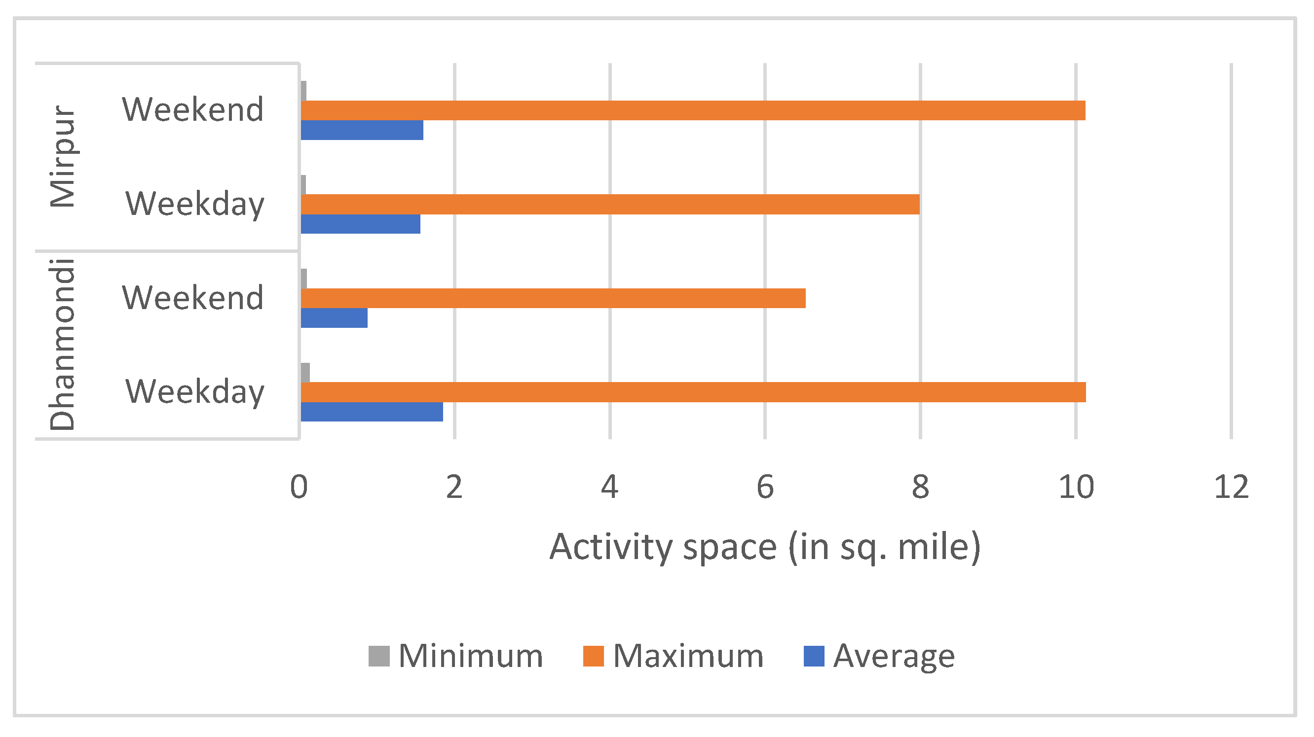
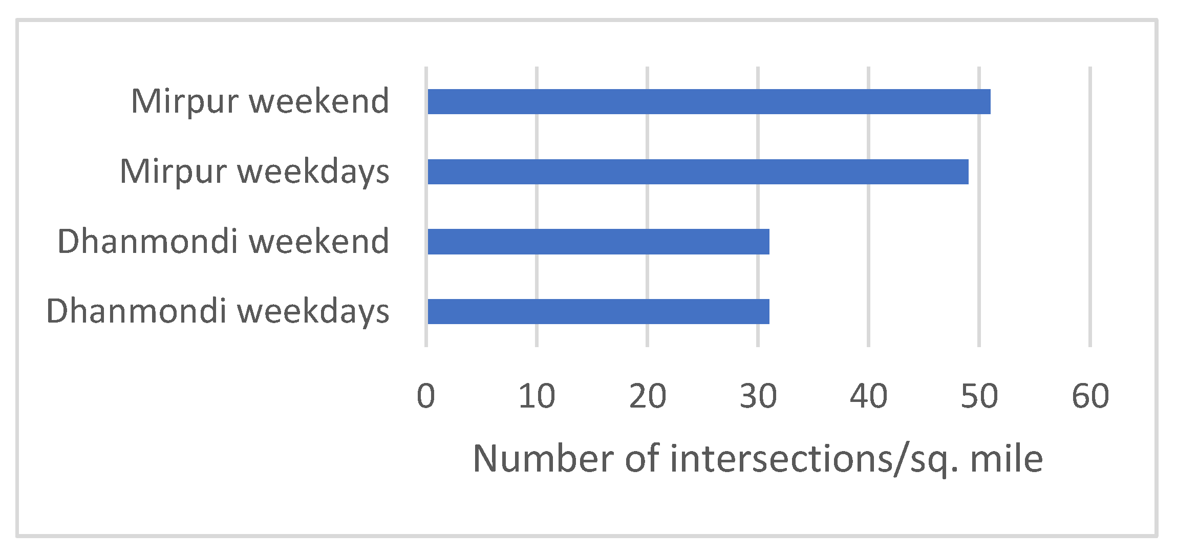
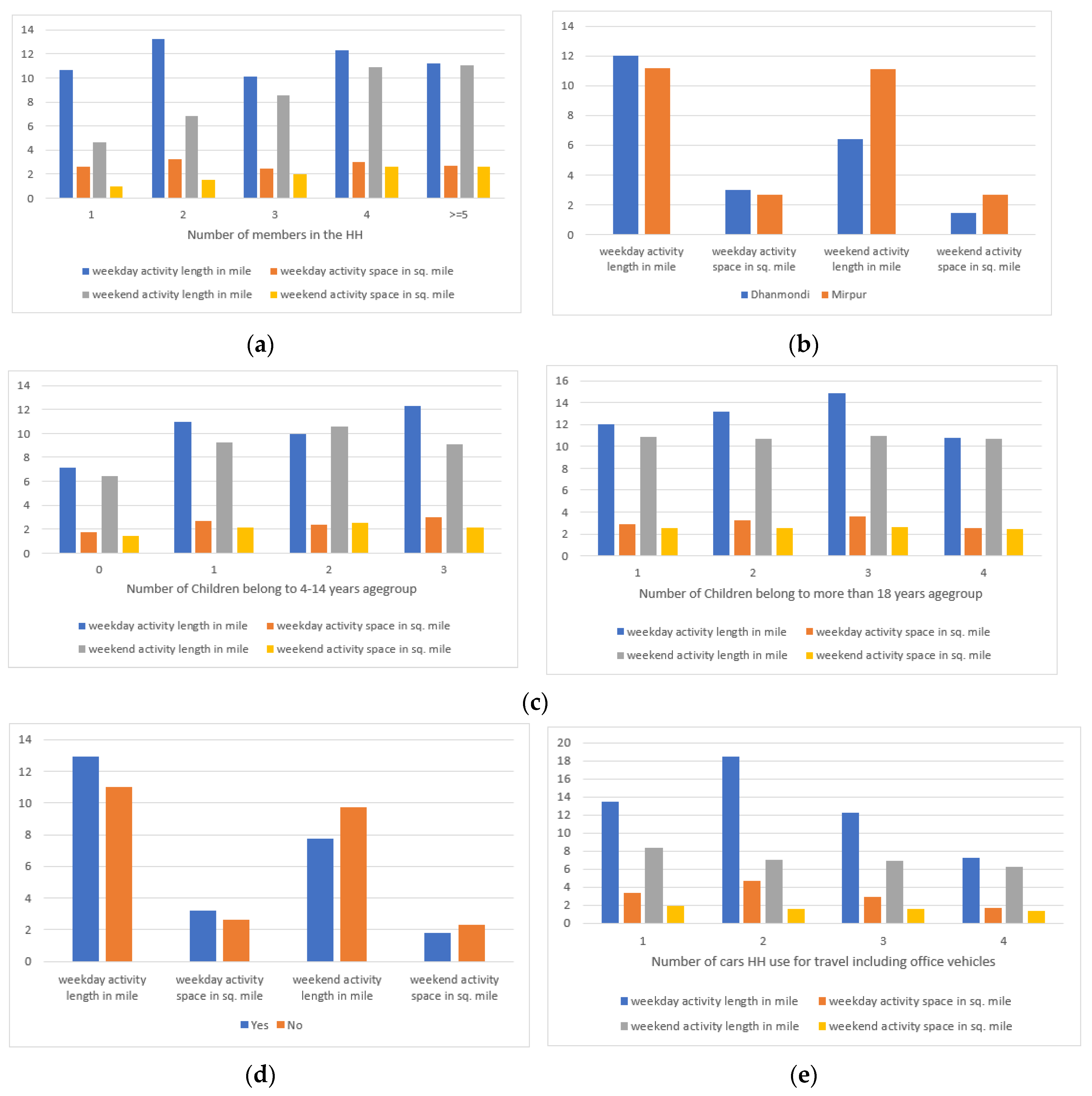
Average weekday activity space for the respondents from Dhanmondi (1.85 sq. miles) was larger than that of respondents from Mirpur (1.55 sq. miles) which indicates slightly more dispersed activity locations for Dhanmondi over Mirpur during weekdays. On the other hand, average weekend activity space for the respondents from Mirpur (1.6 sq. miles) was much larger than that of respondents from Dhanmondi (0.88 sq. miles). An initial hypothesis regarding this finding was that the Mirpur area is predominantly residential, with less commercial and other facilities, and therefore, Mirpur respondents needed to travel greater distances to satisfy their weekend needs as people travel for shopping etc. in commercial areas during weekends. In the case of road connectivity, Mirpur showed relatively better connectivity than Dhanmondi, displaying more intersections per square mile within a respondent’s activity areas.
Cronbach’s alpha values derived from confirmatory factor analysis for most of the attitude-based factors were found as more than 70% which indicates sufficient internal reliability. So, it can be said that selection of perception related statements was satisfactory for this study. Among the 10 attitudinal factors, five factors (perceived neighborhood amenities, car attachment, monetary concerns, transit preferences, perceived daily travel area and environmental concern) showed a significant impact on weekend activity space of individual respondents but no significant influence on weekday activity space.
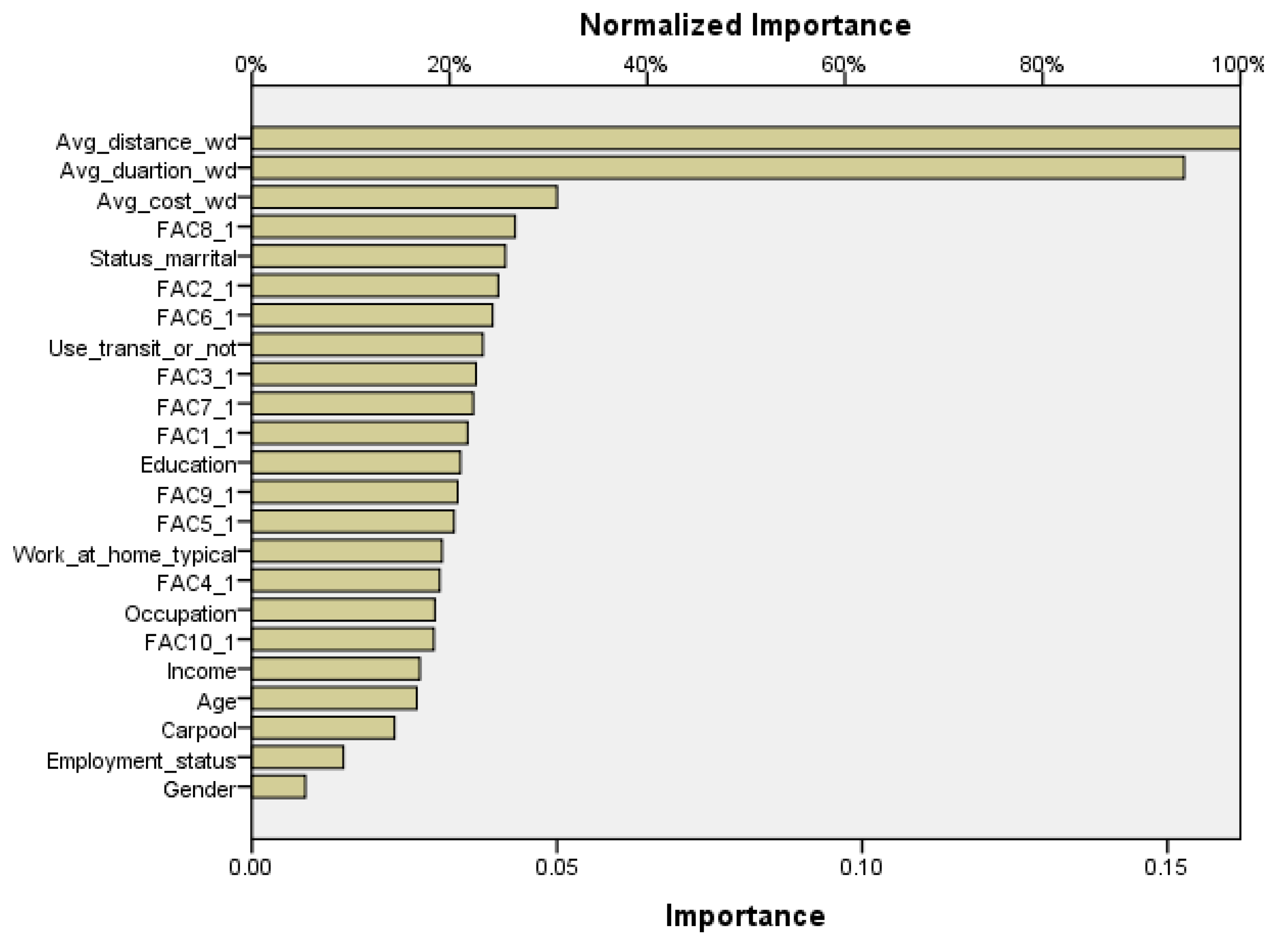
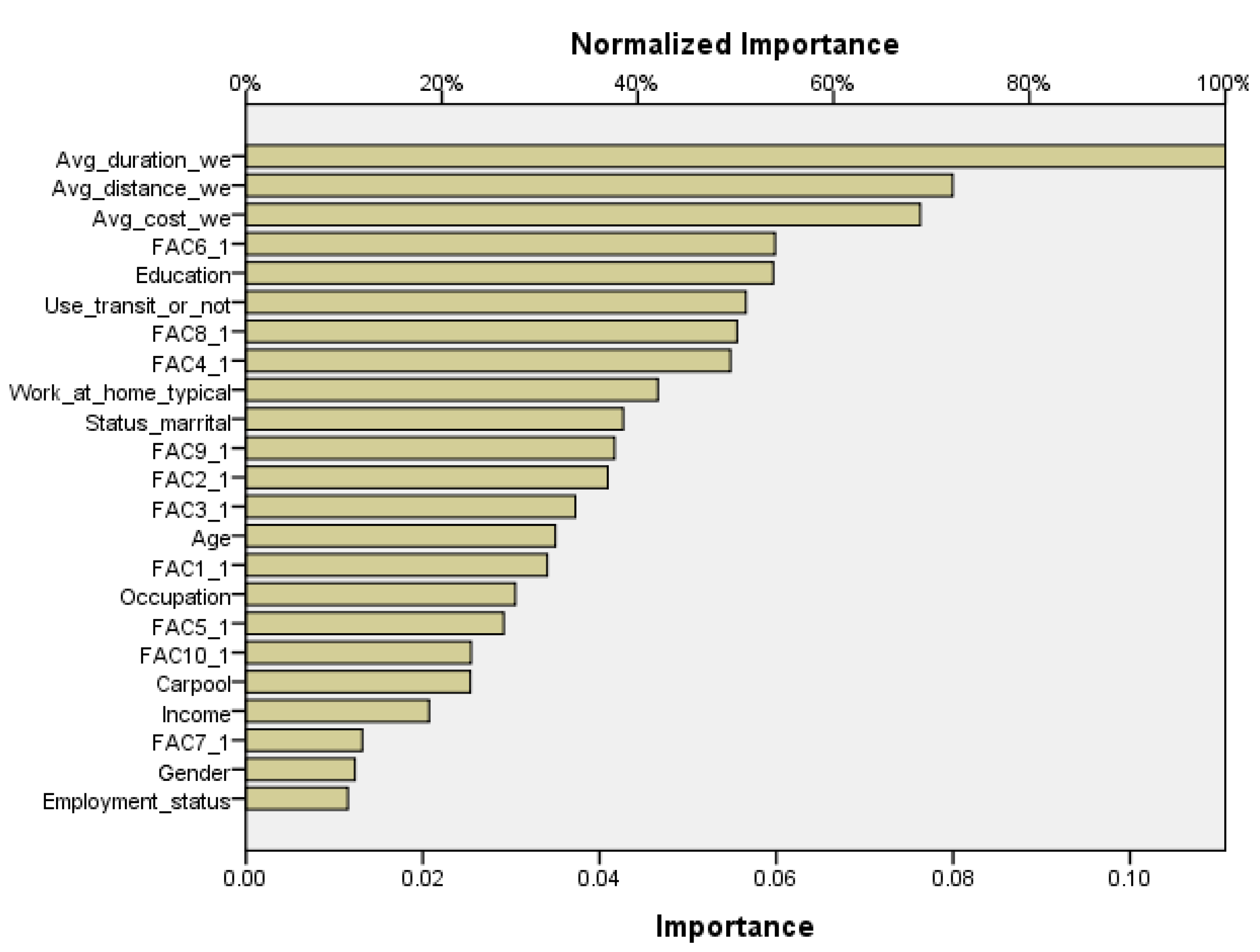
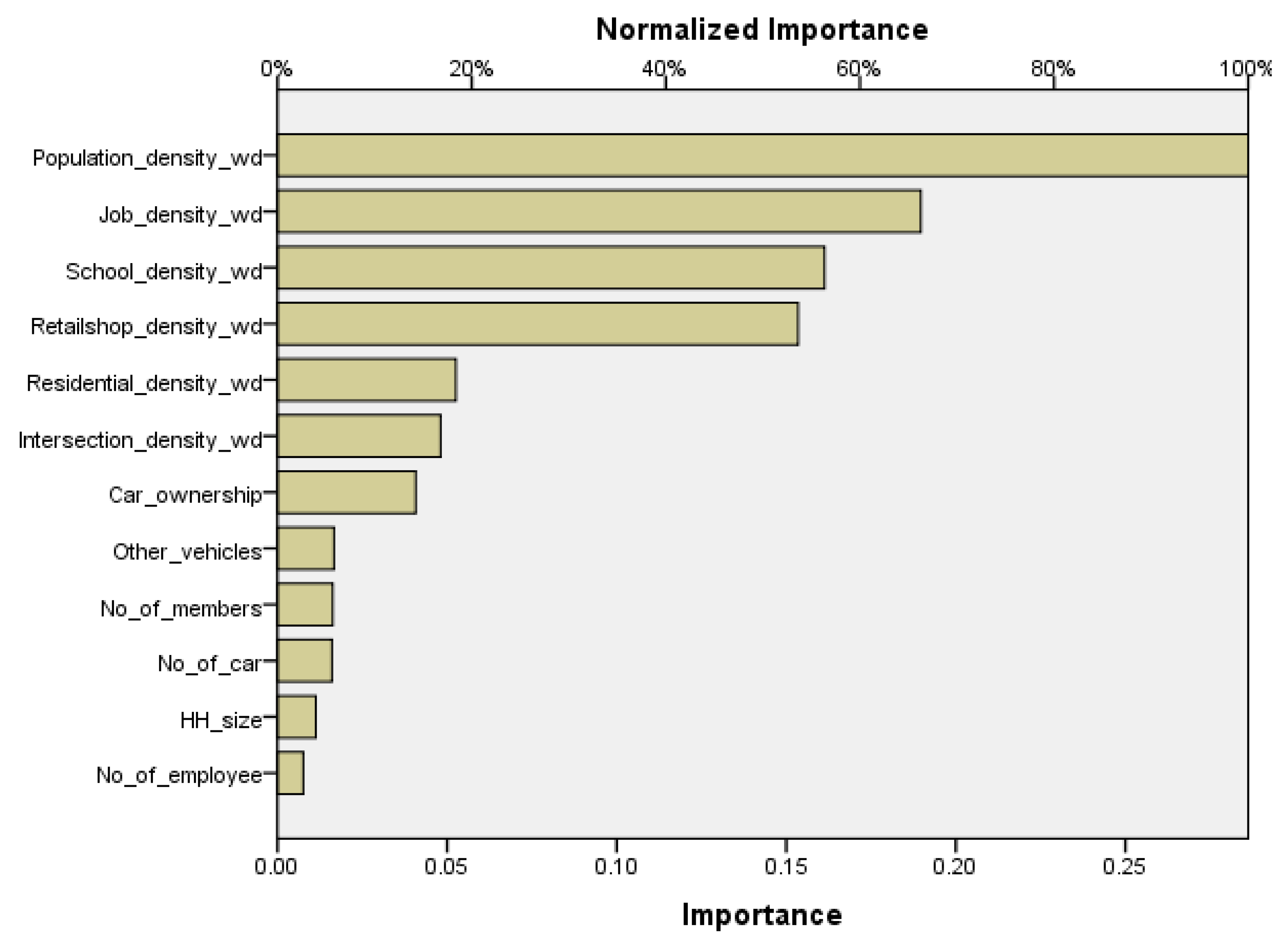
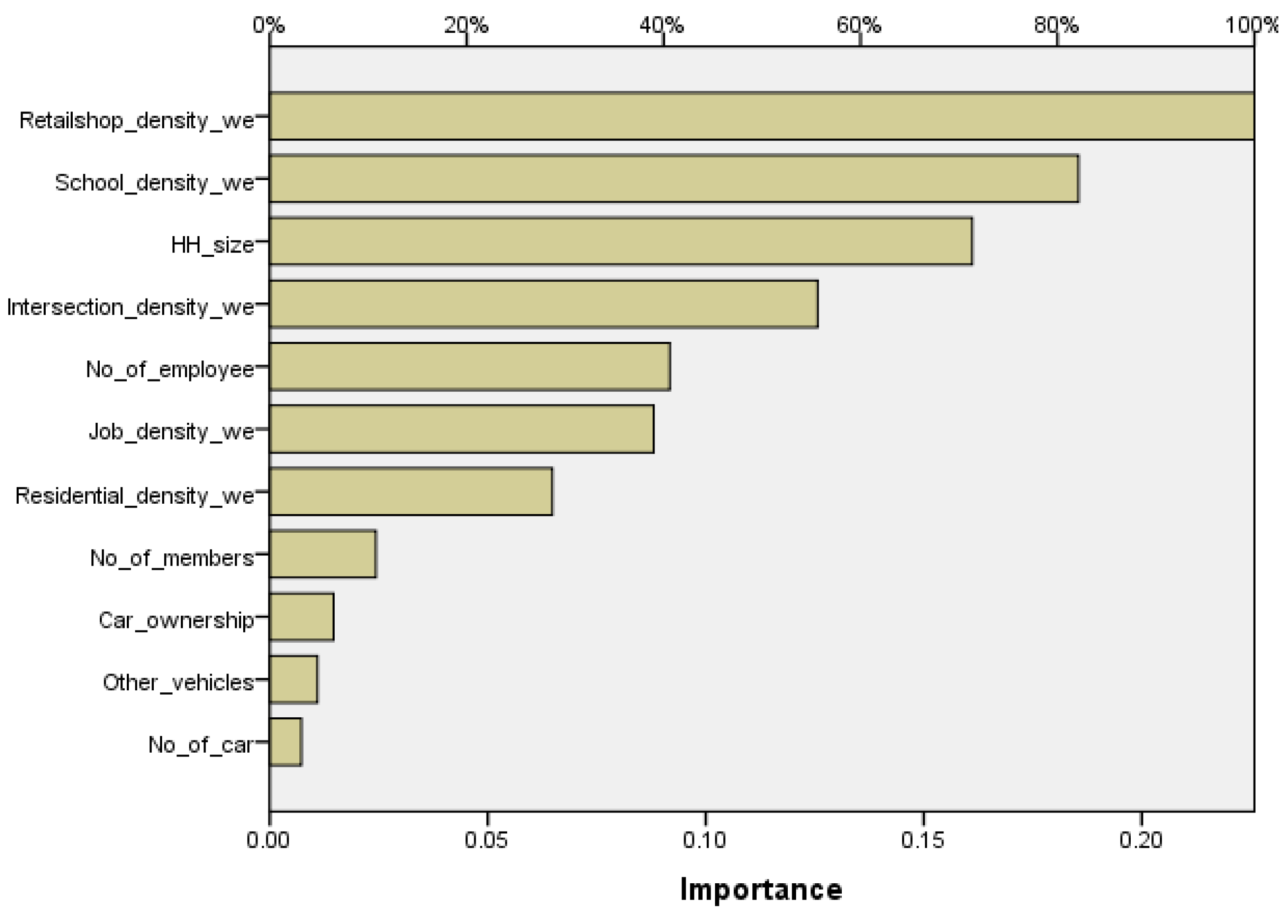
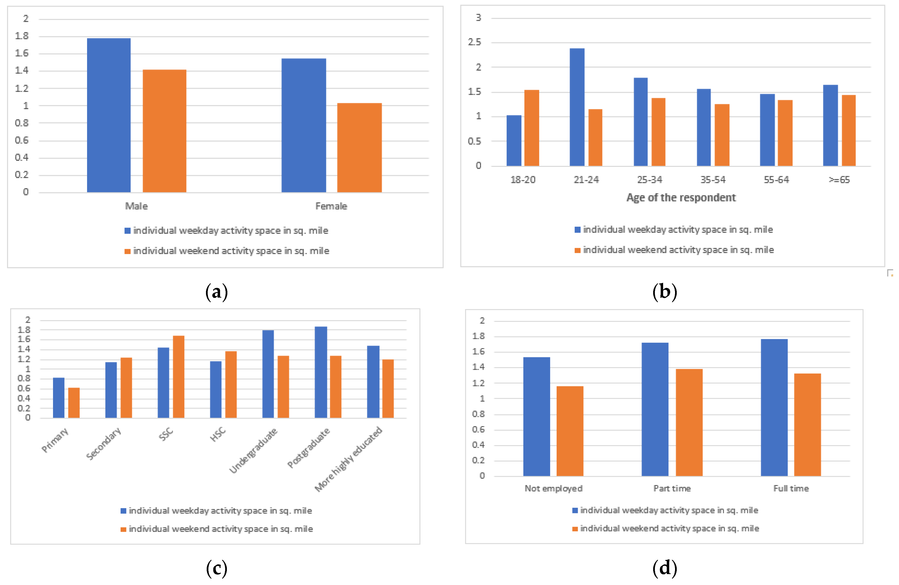
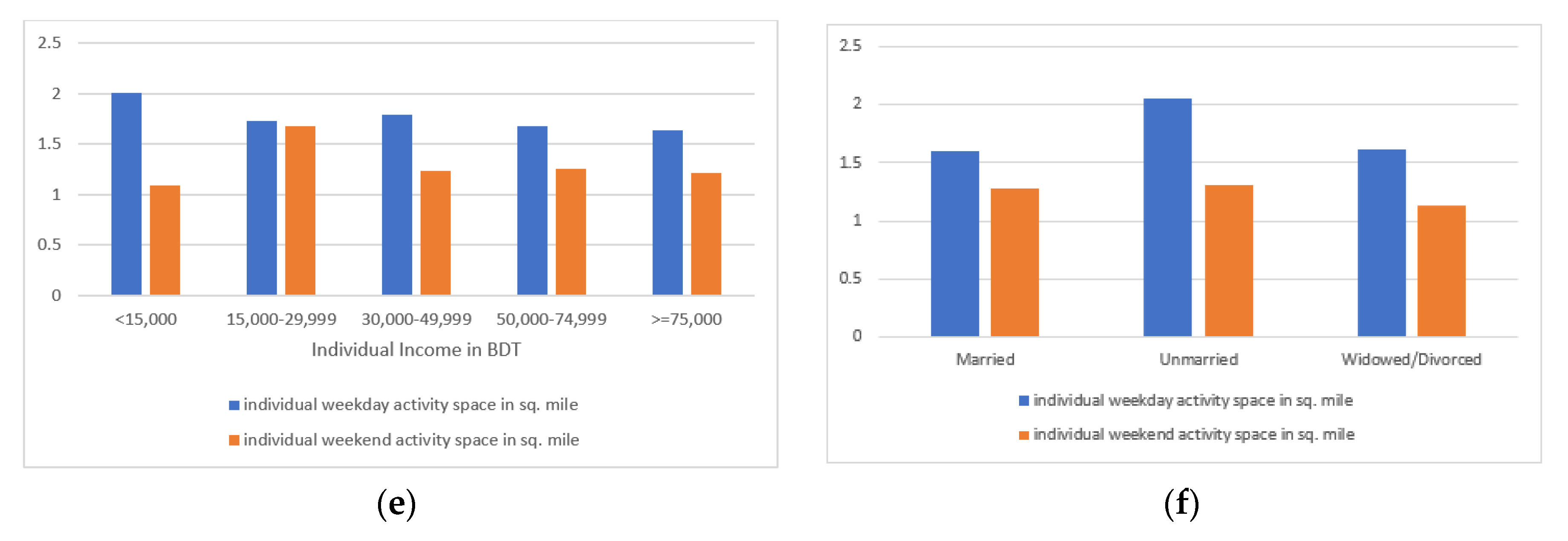
In case of an individual respondent’s weekday and weekend model developed by an artificial neural network, bias towards trip characteristics (distance, duration, and cost) were found in the results. Individual models showed relatively more error percentage in explaining the dependent variable in comparison to the household models. On the other hand, individual models developed with the help of multiple regression analysis also showed significance of the trip-related variables (travel distance, duration etc.), but apart from that in the weekday model, young age group and lower income group significantly affected the dependent variable (activity space) and transit use, lower-middle income group (monthly income USD 177–354) were found as significant variables in the case of the weekend model. From the co-efficient values, it was found that female, unemployed, and retired respondents; comparatively young age group, high income group, lower education level, and single persons had a smaller activity space during weekdays. In the case of weekend travel, people who worked from home, females, unemployed, govt. service holder and retired respondents; aged people, both low- and high-income group, both lower and more highly educated people and unmarried (single) respondents had a smaller activity space.
While interpreting household model developed for weekdays and weekends, household models were found to be much better in terms of model fit (regression) and minimum error level (ANN model) in comparison to the individual ones. Model estimation results showed that mainly D variables (density and destination accessibility) and household size were consistently the most significant explanatory variables that influenced the magnitude of the household’s activity space indices during weekends. D variables were not used in individual models as individual socio-economic characteristics, attitudes, travel/trip characteristics were included as explanatory variables in that model. On the other hand, in the household model, household characteristics, land use characteristics (urban form: D variables), population characteristics were included as these features are similar for all members of one household as these are location-based variables (spatial variable). Higher density population and higher density of offices (job locations) within a household’s activity space decreased the weekday activity space. Besides these, better traffic conditions with well-connected road networks and large household sizes also reduced activity space of households during weekdays. Like with the weekday findings, D variables (higher density of offices, schools, shops) and more car use reduced activity space during weekend for households. Unlike the weekday findings, smaller households were found to have a smaller activity space for weekends.
While interpreting the model summary of the four multiple regression models developed in this paper, comparatively low R2 and adjusted R2 values were observed in the case of the first two models. It can be explained since attitude-related variables (subjective behavior of people) were included as predictor (independent) variables for the first two models, while land use characteristics were included in the latter two models and represent a better model fit. R-square, even when small, can be significantly different from 0, indicating that the regression model has statistically significant explanatory power. A small R-square could have important implications. In social or behavioral science, to examine the effectiveness of a factor, the size of R2 does not matter.
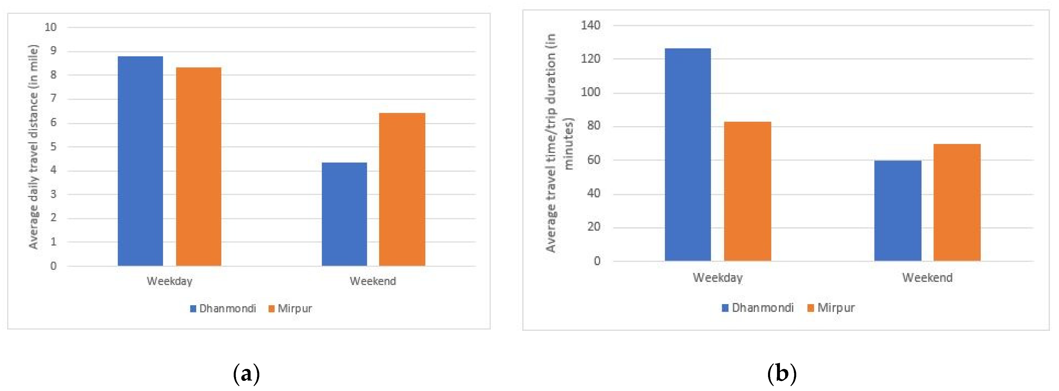
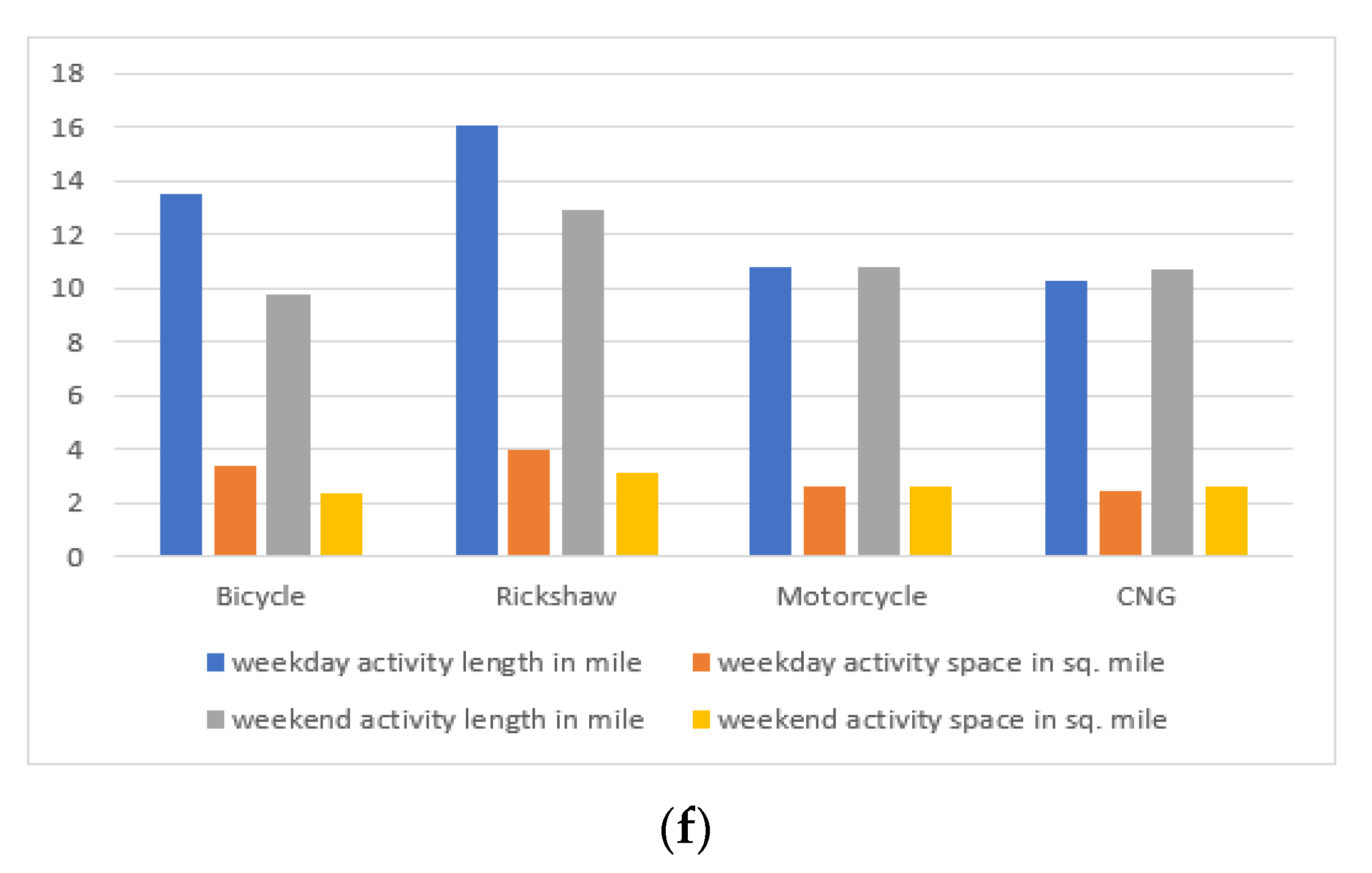
From the accessibility of opportunities analysis, each household was found to have at least one school, hospital, retail shop and restaurant facility for both weekday and weekend trips within their activity space. Using a travel diary collected on seven consecutive days in the DMA area, we examined weekday-to-weekend variability of individual and household activity spaces. Furthermore, household and individuals’ interpersonal and intrapersonal variability in activity space indices were examined systematically. The RNB of activity locations increased during the weekday. However. households with two dependent children from the 4–14 years age group, with two elderly persons above 65 years, with motorized vehicles ownership (motorcycle and CNG ownership, not car) and without-car households tended to have activity centroids farther from their home locations during weekends. Dhanmondi respondents had a larger activity space during weekdays in comparison to the Mirpur weekday activity space. Additionally, weekday-to-weekend variability was much larger in Dhanmondi in comparison to Mirpur. Single-person or more-than-two-member households had a smaller activity space during weekdays. Individual day-to-day variability was less during weekdays than at the weekend. Male respondents were found to have a larger activity space in comparison to females during both weekdays and weekends which is somewhat expected due to the social context of Bangladesh. Comparatively young age group respondents with an education level of a higher secondary degree visited more distant places during weekends in comparison to weekdays. High-income respondents had lower activity space values in comparison to other income category people and visited activity locations farther from home on weekdays in comparison to their weekend travel.
In our case of a developing country, it was found that D variables and travel, household characteristics were more significant than socioeconomic characteristics and perceptions (personal attitude) in shaping daily activity locations across urban space. Household activity space models showed better model fit than individual models. This conclusion should, however, be treated with caution as context varies from place to place. Even though objective (quantitative) measures were proved to be more powerful rather than subjective human behavior and characteristics here, we cannot say that these findings can also be generalized for developed world cities. It is indeed true that most studies on activity spaces are Western-based, and this study might add new insights from a developing country like Bangladesh; however, the extent to which the findings of this study are different or comparable to those Western studies requires a similar detailed study. Some suggestions for further work are as follows: study sub-area-wise models can be developed and household characteristics (HH size, number of cars used etc.) can be included as predictors in an individual model which was not done in this paper.
The difference between the activity space measurement methods is mainly related to the street pattern. For grid road networks (high connectivity), the difference between the circular method and network-based methods is moderate with the latter offering only slight improvements in the representation of a local neighborhood. However, for irregular road networks (lower connectivity) in suburban settings, the circular method becomes a much less useful approximation compared to those that account for the structure of the road network. As this study’s two sub-areas hold both characteristics regarding road networks (Dhanmondi with grid iron pattern and Mirpur with irregular road network connectivity), the use of shortest path network with road network buffer as an activity space measurement tool can be said to be sufficient. Two major limitations of some activity space studies are mentioned in Chen and Akar (2016) [53]. One limitation is related to the residential self-selection effect. If the survey database does not contain individual panel data or have attitudinal variables, the ability to deal with residential self-selection issues will be limited. However, the inclusion of socio demographics can control for this effect to some extent. Another limitation is not to have specific longitudes and latitudes of origins, destinations, and residential locations provided by survey organization. This restriction affects the accuracy of calculating activity spaces to a certain degree. However, the grid-cell approach can provide an alternative for operationalizing activity space when data are limited. However, our study database does not have any of these limitations.

Supplementary Materials

Author Contributions

Conceptualization, N.S. and D.H.; data curation, N.S.; formal analysis, N.S.; funding acquisition, D.H.; investigation, N.S.; methodology, N.S.; project administration, D.H.; resources, N.S. and D.H.; software, N.S.; supervision, D.H.; validation, D.H.; visualization, N.S.; writing—original draft, N.S.; writing—review and editing, D.H. All authors have read and agreed to the published version of the manuscript.

Funding

This research received no external funding.

Acknowledgments

The authors would like to express gratitude to Stephen G. Ritchie, Jean-Daniel Saphores, Jae Hong Kim, and Teresa A. Dalton from University of California, Irvine for acting as the Candidacy committee members for this ongoing PhD research and providing valuable suggestions during the dissertation proposal presentation. Moreover, we would like to thank undergraduate students of Bangladesh University of Engineering & Technology, Jahangirnagar University, Pabna University of Science & Technology, Rajshahi University of Engineering & Technology and American International University of Bangladesh for their support and contribution in the extensive Household Questionnaire Survey and Travel Log data collection.

Conflicts of Interest

The authors declare no conflict of interest.

References

  1. Akharuzzaman, M. Urbanization and Environmental Concept of Dhaka City Bangladesh. In Urban Study Seminar; Fukuoka Asian Urban Research Centre: Fukuoka, Japan; Available online: http://urc.or.jp/wp-content/uploads/2014/06/0612_bangla_2.pdf (accessed on 31 October 2020).
  2. Ahmed, R.M. A Study on the Morphological Transformation and the Emerging Spatial Patterns of Spontaneous Retail Development in Bir Uttam Khademul Bashar Road, Banani, Dhaka. Post Graduate Dissertations Thesis of Department of Architecture, Bangladesh University of Engineering & Technology (BUET), Dhaka, Bangladesh, 25 March 2019. Available online: http://lib.buet.ac.bd:8080/xmlui/handle/123456789/5366 (accessed on 15 June 2020).
  3. Arai, A.; Shibasaki, R. Estimation of human mobility patterns and attributes analyzing anonymized mobile phone CDR: Developing real-time census from crowds of greater Dhaka. In CEUR Workshop Proceedings; The University of Tokyo: Tokyo, Japan, 2013; Available online: http://ceur-ws.org/Vol-1136/paper2.pdf (accessed on 2 December 2020).
  4. Byomkesh, T.; Nakagoshi, N.; Dewan, A.M. Urbanization and green space dynamics in Greater Dhaka, Bangladesh. Landsc. Ecol. Eng. 2012, 8, 45–58. [Google Scholar] [CrossRef]
  5. Islam, S. Middle-income Women in Dhaka City: Gender and Activity Space. Master’s Thesis, University of Durham, Durham, UK, 1995. Available online: http://etheses.dur.ac.uk/5235/%0A (accessed on 11 June 2020).
  6. Rahman, M.S. Understanding the Linkages of Travel Behavior with Socioeconomic Characteristics and Spatial Environments in Dhaka City and Urban Transport Policy Applications. Master’s Thesis, Hiroshima University, Hiroshima, Japan, September 2008. Available online: http://sr-milan.tripod.com/Master_Thesis.pdf (accessed on 11 June 2020).
  7. Roushan, N. In the Shadow: A Study for Utilization of Space under Flyovers in Dhaka. Graduate Dissertations Bachelor of Architecture of Department of Architecture, BRAC University, Dhaka, Bangladesh, 2013. Available online: http://10.0.4.191/02705346-2209943%5Cnhttps://login.e.bibl.liu.se/login?url=https://0-search-ebscohost-com.brum.beds.ac.uk/login.aspx?direct=true&db=aph&AN=90518293&site=eds-live&scope=site (accessed on 22 May 2020).
  8. Uddin, R.; Burton, N.W.; Khan, A. Perceived environmental barriers to physical activity in young adults in Dhaka City, Bangladesh-does gender matter? Int. Health 2018, 10, 40–46. [Google Scholar] [CrossRef] [PubMed] [Green Version]
  9. Islam, M.; Mahmud, A.; Islam, S.M.D. Open space management of Dhaka city, Bangladesh: A case study on parks and playgrounds. Int. Res. J. Environ. Sci. 2015, 4, 118–126. [Google Scholar]
  10. Gomes, C.D. Study of Spatial Organization of the Contemporary Residential Apartments in Dhaka With Special Attention to Gender Aspect. Post Graduate Dissertations Thesis of Department of Architecture, BUET, Dhaka, Bangladesh, December 2014. Available online: http://lib.buet.ac.bd:8080/xmlui/handle/123456789/3124 (accessed on 15 May 2020).
  11. Gomes, C.D. Visibility effecting gender aspects in middle income group apartments in Dhaka. In Proceedings of the SSS 2015–10th International Space Syntax Symposium, London, UK, 13–17 July 2015; pp. 1–15. [Google Scholar]
  12. Sharmeen, N.; Houston, D. Spatial characteristics and activity space pattern analysis of Dhaka city, Bangladesh. Urban. Sci. 2019, 1, 36. [Google Scholar] [CrossRef] [Green Version]
  13. Järv, O.; Ahas, R.; Witlox, F. Understanding monthly variability in human activity spaces: A twelve-month study using mobile phone call detail records. Transp. Res. Part. C. 2014, 38, 122–135. [Google Scholar] [CrossRef]
  14. Oliver, L.N.; Schuurman, N.; Hall, A.W. Comparing circular and network buffers to examine the influence of land use on walking for leisure and errands. Int. J. Health Geogr. 2007, 11, 1–11. [Google Scholar] [CrossRef] [Green Version]
  15. Lee, N.C.; Voss, C.; Frazer, A.D.; Hirsch, J.A.; Mckay, H.A.; Winters, M. Does activity space size in fluence physical activity levels of adolescents? A GPS study of an urban environment. PMEDR 2016, 3, 75–78. [Google Scholar] [CrossRef] [Green Version]
  16. Tana; Kwan, M.-P.; Chai, Y. Urban form, car ownership and activity space in inner suburbs: A comparison between Beijing (China) and Chicago (United States). Urban. Stud. 2016, 53, 1784–1802. [Google Scholar] [CrossRef]
  17. Vich, G.; Miralles-guasch, C. Suburban commuting and activity spaces: Using smartphone tracking data to understand the spatial extent of travel behavior. Geogr. J. 2017, 183, 426–439. [Google Scholar] [CrossRef]
  18. Guerra, E.; Caudillo, C.; Goytia, C.; Quiros, T.P.; Rodriguez, C. Residential location, urban form, and household transportation spending in Greater Buenos Aires. J. Transp. Geogr. 2018, 72, 76–85. [Google Scholar] [CrossRef]
  19. Yuan, Y.; Raubal, M. Analyzing the distribution of human activity space from mobile phone usage: An individual and urban-oriented study. Int. J. Geogr. Info. Sci. 2016, 30, 1594–1621. [Google Scholar] [CrossRef]
  20. Handy, S.L.; Boarnet, M.G.; Ewing, R.; Killingsworth, R.E. How the built environment affects physical activity views from urban planning. Am. J. Prev. Med. 2002, 23. [Google Scholar] [CrossRef]
  21. Berke, E.M.; Koepsell, T.D.; Moudon, A.V.; Hoskins, R.E.; Larson, E.B. Association of the built environment with physical activity and obesity in older persons. Am. J. Publ. Health 2007, 97, 486–492. [Google Scholar] [CrossRef] [PubMed]
  22. Kirtland, K.A.; Porter, D.E.; Addy, C.L.; Neet, M.J.; Williams, J.E.; Sharpe, P.A.; Ainsworth, B.E. Perception versus reality. Am. J. Prev. Med. 2003, 24, 323–331. [Google Scholar] [CrossRef]
  23. Nelson, M.C.; Gordon-larsen, P.; Song, Y.; Popkin, B.M. Associations with adolescent overweight and activity. Am. J. Prev. Med. 2006, 31. [Google Scholar] [CrossRef]
  24. Rutt, C.; Koleman, K. Examining the realtionships among built environment, physical activity, and body mass index in El Paso, TX. Prev. Med. 2005, 40, 831–841. [Google Scholar] [CrossRef]
  25. Schönfelder, S. Urban Rhythms–modelling the Rhythms of Individual Travel Behavior. Doctoral Thesis, University of Dortmund, ETH Zurich, Rämistrasse, Zürich, 2006. Available online: https://0-doi-org.brum.beds.ac.uk/10.3929/ethz-a-005320162 (accessed on 15 January 2017).
  26. Dharmowijoyo, D.B.E.; Susilo, Y.O.; Karlström, A. Day-to-day interpersonal and intrapersonal variability of individuals activity spaces in a developing country. Environ. Plan. B: Plan. Des. 2014, 41, 1063–1076. [Google Scholar] [CrossRef]
  27. Dieleman, F.M.; Dijst, M.; Burghouwt, G. Urban form and travel behavior: Micro-level household attributes and residential context. Urban. Stud. 2002, 39, 507–527. [Google Scholar] [CrossRef]
  28. Wilson, C. Activity patterns in space and time: Calculating representative Hagerstrand trajectories. Transportation 2008, 35, 485–499. [Google Scholar] [CrossRef]
  29. Kim, H.-M.; Kwan, M.-P. Space-time accessibility measures: A geocomputational algorithm with a focus on the feasible opportunity set and possible activity duration. J. Geogr. Sys. 2003, 5, 71–91. [Google Scholar] [CrossRef]
  30. Kwan, M.-P. Space-time, and integral measures of individual accessibility: A comparative anal ysis using a point-based framework. Geogr. Anal. 1998, 30, 191–216. [Google Scholar] [CrossRef]
  31. Kwan, M.-P. Gender, the homework and space-time patterns pattern. Econ. Geogr. 1999, 74, 370–394. [Google Scholar] [CrossRef]
  32. Kwan, M.-P. Gender, and individual access to urban opportunities: A study using space–timemeasures. Prof. Geogr. 1999, 51, 210–227. [Google Scholar] [CrossRef]
  33. Kwan, M.-P. Gender differences in space-time constraints. Area 2000, 32, 145–156. [Google Scholar] [CrossRef]
  34. Weber, J.; Kwan, M. Bringing time back in: A study on the influence of travel time variations and facility opening hours on individual accessibility bringing time back in: A study on the influence. Prof. Geogr. 2002, 54, 226–240. [Google Scholar] [CrossRef]
  35. Buliung, R.N.; Kanaroglou, P.S. A GIS toolkit for exploring geographies of household activity/travel behavior. J. Transp. Geogr. 2006, 14, 35–51. [Google Scholar] [CrossRef]
  36. Buliung, R.N.; Kanaroglou, P.S. Urban form and household activity-travel behavior. Growth Change 2006, 37, 172–199. [Google Scholar] [CrossRef]
  37. Dharmowijoyo, D.B.E.; Susilo, Y.O.; Karlstrom, A. Day-to-day variability in traveller’s activity-travel patterns in the Jakarta metropolitan area. Transportation 2016, 43, 601–621. [Google Scholar] [CrossRef]
  38. Holliday, K.M.; Howard, A.G.; Emch, M.; Rodríguez, D.A.; Evenson, K.R. Are buffers around home representative of physical activity spaces among adults? Health Place 2017, 45, 181–188. [Google Scholar] [CrossRef] [Green Version]
  39. Mannan, S.M.; Karim, M.M. Current state of the mobility of the urban dwellers in Greater Dhaka. In Proceedings of the 94th Annual Conference and Exhibition of Air and Waste Management Association, Orlando, FL, USA, 24–28 June 2001. [Google Scholar]
  40. Li, R.; Tong, D. Constructing human activity spaces: A new approach incorporating complex urban activity-travel. J. Transp. Geogr. 2016, 56, 23–35. [Google Scholar] [CrossRef]
  41. Park, K.; Ewing, R.; Sabouri, S.; Larsen, J. Street life and the built environment in an auto-oriented US region. Cities 2019, 88, 243–251. [Google Scholar] [CrossRef]
  42. Houston, D.; Lo, A. Do compact, accessible, and walkable communities promote gender equality? J. Transp. Geogr. 2018, 68, 42–54. [Google Scholar] [CrossRef]
  43. Jain, K.; Payal. A review study on urban planning & artificial intelligence. Int. J. Soft Comput. Eng. 2011, 1, 101–104. [Google Scholar]
  44. Maithani, S.; Jain, R.K.; Arora, M.K. An artificial neural network based approach for modelling urban spatial growth. Itpi J. 2007, 4, 43–51. [Google Scholar]
  45. RAJUK. Draft Dhaka Structure Plan Report 2016–2035 (Full Volume). 2015. Available online: https://www.academia.edu/31508051/_Draft_Dhaka_Structure_Plan_Report_2016_2035_Full_Volume (accessed on 15 January 2019).
  46. Anable, J. “Complacent Car Addicts” or “Aspiring Environmentalists”? Identifying travel behaviour segments using attitude theory. Transp. Policy 2005, 12, 65–78. [Google Scholar] [CrossRef] [Green Version]
  47. Elias, W.; Shiftan, Y. The influence of individual’s risk perception and attitudes on travel behavior. Transp. Res. Part. A Policy Pract. 2012, 46, 1241–1251. [Google Scholar] [CrossRef]
  48. Horton, F.E.; Reynolds, D.R. Effects of urban spatial structure on individual behavior. Econ. Geogr. 1971, 47, 36–48. [Google Scholar] [CrossRef]
  49. Houston, D.; Boarnet, M.G.; Ferguson, G.; Spears, S. Can compact rail transit corridors transform the automobile city? Planning for more sustainable travel in Los Angeles. Urban. Stud. 2015, 52, 938–959. [Google Scholar] [CrossRef]
  50. Spears, S.; Houston, D.; Boarnet, M.G. Illuminating the unseen in transit use: A framework for examining the effect of attitudes and perceptions on travel behavior. Transp. Res. Part. A Policy Pract. 2013, 58, 40–53. [Google Scholar] [CrossRef]
  51. Wang, T.; Chen, C. Attitudes, mode switching behavior, and the built environment: A longitudinal study in the Puget Sound Region. Transp. Res. Part. A Policy Pract. 2012, 46, 1594–1607. [Google Scholar] [CrossRef]
  52. Hair, J.F.; Black, B.; Babin, B.; Anderson, R.E.; Tatham, R.L. Multivariate Data Analysis (sixth); Pearson Education Inc.: New York, NY, USA, 2006. [Google Scholar]
  53. Chen, N.; Akar, G. Effects of neighborhood types & socio-demographics on activity space. J. Transp. Geogr. 2016, 54, 112–121. [Google Scholar] [CrossRef]
Figure 1. Two study sub-areas: Dhanmondi and Mirpur Thanas in Dhaka Metropolitan Area. Thana: Administrative unit/district containing multiple wards controlled by one specific police station. Ward is a smaller administrative unit representing municipality for electing representatives in local level. DCC: Dhaka City Corporation.
Urbansci 04 00069 g001
Figure 2. Change in people’s perception (preference) with car ownership status change in (a) Dhanmondi and (b) Mirpur area.
Urbansci 04 00069 g002
Figure 3. Descriptive of individual activity space of survey respondents.
Urbansci 04 00069 g003
Figure 4. Trip characteristics of respondents in weekdays and weekend from both study sub-areas. (a) Average daily travel distance and (b) travel time/trip duration.
Urbansci 04 00069 g004
Figure 5. Gender-based comparison of (a) perception and (b) actual behavior in choosing mode to workplace.
Urbansci 04 00069 g005
Figure 6. Day wise percentage of trips by trip purpose.
Urbansci 04 00069 g006
Figure 7. Day-wise modal frequency by number of passengers in different travel modes. HH: human hauler.
Urbansci 04 00069 g007
Figure 8. Visualization of WDAS (Weekday Activity Space) and WEAS (Weekend Activity Space) based on activity locations by SPN with RNB method: (a) an example of a 2 member HH living in Dhanmondi and (b) an example of a 3 member HH living in Mirpur. WEAL: weekend activity length, WDAL: weekday activity length, WEAP: weekend activity point, WDAP: weekday activity point.
Urbansci 04 00069 g008
Figure 9. Aggregate activity space (a) Dhanmondi weekday, (b) Dhanmondi weekend, (c) Mirpur weekday, and (d) Mirpur weekend (a comparative illustration).
Urbansci 04 00069 g009
Figure 10. Study sub-area-wise intersection density during weekdays and weekends.
Urbansci 04 00069 g010
Figure 11. Normalized importance.
Urbansci 04 00069 g011
Figure 12. Normalized importance.
Urbansci 04 00069 g012
Figure 13. Network.
Figure 13. Network.
Urbansci 04 00069 g013
Figure 14. Normalized importance.
Urbansci 04 00069 g014
Figure 15. Normalized importance.
Urbansci 04 00069 g015
Figure 16. The weekday-to-weekend variability of household activity space indices. (a) AS values by HH size; (b) AS values by study sub-areas; (c) AS values by presence of children in household from different age categories; (d) AS values by car ownership status; (e) AS values by number of cars used; (f) AS values by another vehicle ownership.
Urbansci 04 00069 g016aUrbansci 04 00069 g016b
Figure 17. The weekday-to-weekend variability of individual activity space indices. USD 1 is equivalent to BDT 84.77 (Bangladeshi Taka) as of July 7, 2020. (a) AS values by gender; (b) AS values by age; (c) AS values by education level; (d) AS values by employment status; (e) AS values by individual income level; (f) AS values by marital status.
Urbansci 04 00069 g017aUrbansci 04 00069 g017b
Table 1. Area-wise independent sample T test results for some variables. Df: degree of freedom. HH: Household.
Study Sub-AreaMeanFSig.tdfSig. (2-Tailed)
HH sizeDhanmondi3.010.7160.398−7.1139870.000
Mirpur3.50 −7.109975.5310.000
Number of employed persons in the HHDhanmondi1.8746.3270.0003.3489840.001
Mirpur1.79 3.353956.4800.001
Number of cars HH use for travel including office vehiclesDhanmondi1.2753.2100.0003.3202910.001
Mirpur1.07 4.216212.4340.000
Number of Children belong to 4–14 yearsDhanmondi1.1417.4430.000−2.2613720.024
Mirpur1.25 −2.330366.8430.020
Number of Elderly persons in the HH > 65 yearsDhanmondi1.180.0080.928−0.0451190.964
Mirpur1.18 −0.04574.8400.964
Daily average distance (km)Dhanmondi12.612.2790.1310.18017390.857
Mirpur12.49 0.1821732.0920.856
Daily average travel time (minute)Dhanmondi114.0558.5860.00011.29917770.000
Mirpur78.85 11.1681580.6070.000
Daily average travel cost (BDT)Dhanmondi100.7726.2360.0007.69714240.000
Mirpur60.37 7.5201197.9800.000
Table 2. Descriptive statistics of household activity length using shortest path network (SPN) method and HH activity space/area using road network buffer (RNB) method.
Activity Length (in mile)Activity Space (in sq. mile)
Avg 1Max 2Min 3Avg 1Max 2Min 3
DhanmondiWeekday12.01742.0421.8282.98410.6290.262
Weekend6.38426.841.6751.4377.07410.222
MirpurWeekday11.16439.3581.6672.6519.8750.22
Weekend11.09442.3731.6612.64410.7940.219
1 Average; 2 Maximum; 3 Minimum.
Table 3. Dimension Reduction: Factor Analysis.
KMO and Bartlett’s Test
Kaiser–Meyer–Olkin Measure of Sampling Adequacy0.856
Bartlett’s Test of SphericityApprox. Chi-Square11,926.151
df630
Sig.0.000
Table 4. Measures for built form indicators used in this study.
IndicatorsMeasures
Built form indicatorsDiversity
Entropy index (land use diversity)
Design
Number of intersections within the activity area of each respondent (number of junctions >3 considered as one intersection)
Density
Job/employment density (number of offices within the activity area of each respondent)
Population density 1 (ward wise population density per sq. mile within the activity area of each respondent). This is a socio-demographic variable not a built environment indicator.
Residential density (number of residential homes within the activity area of each respondent)
Destination Accessibility
Respondent’s accessibility to urban opportunities/service facilities (number of opportunities within the activity area of each respondent). Here, two opportunities (schools and retail shops) are being considered.
1 Population density is a socio-demographic indicator not a built environmental characteristic.
Table 5. Model Summary.
ModelRR SquareAdjusted R SquareStd. Error of the EstimateChange Statistics
R Square ChangeF Changedf1df2Sig. F Change
10.526 a0.2770.2361.220250.2776.852325730.000
a Predictors.
Table 6. ANOVA Table.
ANOVA b
ModelSum of SquaresdfMean SquareFSig.
1Regression326.4853210.2036.8520.000 a
Residual853.2105731.489
Total1179.695605
a Predictors; b Dependent Variable.
Table 7. Model Summary.
ModelRR SquareAdjusted R SquareStd. Error of the EstimateChange Statistics
R Square ChangeF Changedf1df2Sig. F Change
10.581 a0.3370.2951.085370.3378.090325090.000
a. Predictors.
Table 8. ANOVA Table.
ANOVA b
ModelSum of SquaresdfMean SquareFSig.
1Regression304.972329.5308.0900.000 a
Residual599.6125091.178
Total904.584541
a Predictors; b Dependent Variable.
Table 9. Model Summary.
ModelRR SquareAdjusted R SquareStd. Error of the EstimateChange Statistics
R Square ChangeF Changedf1df2Sig. F Change
10.739 a0.5470.5231.591370.54723.249142700.000
a Predictors.
Table 10. ANOVA Table.
ANOVA b
ModelSum of SquaresdfMean SquareFSig.
1Regression824.2751458.87723.2490.000 a
Residual683.7682702.532
Total1508.043284
a Predictors; b Dependent Variable.
Table 11. Model Summary.
ModelRR SquareAdjusted R SquareStd. Error of the EstimateChange Statistics
R Square ChangeF Changedf1df2Sig. F Change
10.727 a0.5280.5031.175910.52821.443122300.000
a Predictors.
Table 12. ANOVA Table.
ANOVA b
ModelSum of SquaresdfMean SquareFSig.
1Regression355.8111229.65121.4430.000 a
Residual318.0382301.383
Total673.849242
a Predictors; b Dependent Variable.
Table 13. Model Summary.
TrainingSum of Squares Error125.440
Relative Error0.619
Stopping Rule Used1 consecutive step(s) with no decrease in error a
Training Time0:00:00.277
TestingSum of Squares Error59.004
Relative Error0.643
Dependent Variable: individual weekday activity space in sq. mile
a Error computations are based on the testing sample.
Table 14. Model Summary.
TrainingSum of Squares Error97.070
Relative Error0.535
Stopping Rule Used1 consecutive step(s) with no decrease in error a
Training Time0:00:00.292
TestingSum of Squares Error72.906
Relative Error0.649
Dependent Variable: individual weekend activity space in sq. mile
a Error computations are based on the testing sample.
Table 15. Model Summary.
TrainingSum of Squares Error2.548
Average Overall Relative Error0.094
Relative Error for Scale Dependentsweekday activity length in mile0.094
weekday activity space in sq. mile0.095
Stopping Rule Used1 consecutive step(s) with no decrease in error a
Training Time0:00:00.004
TestingSum of Squares Error0.614
Average Overall Relative Error0.053
Relative Error for Scale Dependentsweekday activity length in mile0.046
weekday activity space in sq. mile0.059
a Error computations are based on the testing sample.
Table 16. Model Summary.
TrainingSum of Squares Error10.101
Average Overall Relative Error0.439
Relative Error for Scale Dependentsweekend activity length in mile0.504
weekend activity space in sq. mile0.375
Stopping Rule Used1 consecutive step(s) with no decrease in error a
Training Time0:00:00.006
TestingSum of Squares Error2.861
Average Overall Relative Error0.359
Relative Error for Scale Dependentsweekend activity length in mile0.332
weekend activity space in sq. mile0.386
a Error computations are based on the testing sample.
Table 17. Access to opportunities for road network buffer by Dhanmondi and Mirpur respondents for weekday and weekend activity.
Measure of Activity Space
Dhanmondi WeekdayDhanmondi WeekendMirpur WeekdayMirpur Weekend
MMDRMMDRMMDRMMDR
CS363.07353.530–880177.691471–562206.27196.515–597228.212101–665
H243.34214.519–641107.471021–30181.24−720–29588.47780–330
RF3.2620–210.3500–55.0930–2311.89850–48
RS912.4980074–3285515.446365–24171201.781139.528–35161252.83116515–3651
R81.8672.511–26039.08350–12135.89320–13540.5390–119
OS7.6750–335.5420–2576.7520–26163.7520–216
%S100100100100
H10010098.9999.15
RF71.2818.2464.5968.298
RS100100100100
R10099.7199.39699.57
OS89.2178.5362.7861.91
CRS0.420.470.450.44
H0.60.60.720.608
RF0.450.40.220.004
RS0.740.6860.650.618
R0.720.6380.7350.748
OS0.2610.066−0.060.04
S = school, H = hospital, RF = recreational facilities, RS = retail shop, R = restaurants, OS = open space. M = mean, MD = median, R = range. C = count (number of opportunities), % = percent with at least one opportunity, CR = correlation between area and number of opportunities.
Publisher’s Note: MDPI stays neutral with regard to jurisdictional claims in published maps and institutional affiliations.

