Apache Spark SVM for Predicting Obstructive Sleep Apnea

Department of Computer Science, University of West Florida, Pensacola, FL 32548, USA
*
Author to whom correspondence should be addressed.
Big Data Cogn. Comput. 2020, 4(4), 25; https://0-doi-org.brum.beds.ac.uk/10.3390/bdcc4040025
Submission received: 28 August 2020
/
Revised: 10 September 2020
/
Accepted: 16 September 2020
/
Published: 23 September 2020
Abstract
:Obstructive sleep apnea (OSA), a common form of sleep apnea generally caused by a collapse of the upper respiratory airway, is associated with one of the leading causes of death in adults: hypertension, cardiovascular and cerebrovascular disease. In this paper, an algorithm for predicting obstructive sleep apnea episodes based on a spark-based support vector machine (SVM) is proposed. Wavelet decomposition and wavelet reshaping were used to denoise sleep apnea data, and cubic B-type interpolation wavelet transform was used to locate the QRS complex in OSA data. Twelve features were extracted, and SVM was used to predict OSA onset. Different configurations of SVM were compared with the regular, as well as Spark Big Data, frameworks. The results showed that Spark-based kernel SVM performs best, with an accuracy of 90.52% and specificity of 93.4%. Overall, Spark-SVM performed better than regular SVM, and polynomial SVM performed better than linear SVM, both for regular SVM and Spark-SVM.
1. Introduction
Scientific and medical communities believe that sleep’s physiological significance for humans includes aspects of body tissue repair, protein synthesis, cell division, growth hormone secretion, brain function repair, emotion and memory regulation and reorganization, and other important functions. Therefore, patients with sleep apnea not only suffer from poor sleep quality at night, but also tend to have dry mouth and headaches when waking up in the morning [1], and tend to feel restless and suffer from loss of memory [2]. Patients are also prone to drowsiness during the day [1,3], which reduces the work and learning performance and sometimes leads to unexpected events [2,3]. Since most of these symptoms are not unique clinical manifestations of sleep apnea, they are sometimes considered to be normal because a patient has “aged” and are hence often ignored [4,5,6]. Unlike symptoms during the day, patients with sleep apnea often experience loud and habitual snoring at night, or suddenly have difficulty breathing, which causes them to awaken and have frequent urination at night [7].
In addition to the above clinical symptoms, sleep apnea is also highly comorbid with many cardiovascular diseases [1,8], such as high blood pressure [9], heart failure, coronary artery disease and stroke [1,10], during which patients with sleep apnea syndrome develop brain disorders [10]. The chance of stroke increases as much as 3–8 times with sleep apnea [11]. The proportion of patients with sleep apnea who have a stroke can be as high as 43–91% [11,12]. The medical community believes that mechanisms for increasing sleep stroke apnea include hypertension [1], metabolic syndrome, decreased insulin sensitivity and diabetes, abnormal lipid metabolism, increased sympathetic nervous system activity, inflammatory response, and vascular endothelial cells [3]. The complexity and breath of these effects are difficult to fully cover; however, one should be able to confirm that sleep apnea plays an important role in the development of cardiovascular disease [8]. Therefore, an early diagnosis and treatment of sleep respiratory syndrome is important to prevent strokes. Dimsdale et al. [9] has shown that if patients are identified and treated at an early stage, adverse health effects can be reduced. Furthermore, certain neurobehavioral diseases that may have important health and economic implications are related to sleep apnea, including daytime drowsiness and impaired cognitive function, which can lead to motor vehicle crashes and other work-related accidents [11,13].
There are three main types of sleep apnea: central sleep apnea, which has its origins in the central nervous system; obstructive sleep apnea, where the reason for pauses in breathing lie in a respiratory tract obstruction; and mixed sleep apnea, in which both of the other two reasons may be present. This paper focuses on obstructive sleep apnea (OSA).
Advances in wearable sensors and “big data” predictive analytics technology have been driving the use of point-in-time technology for the treatment of OSA. A variety of position adjustment beds and nerve stimulation devices are available for the treatment of OSA. These devices use biomedical sensors that collect signals such as ECG, EMG and breath, and extract the corresponding signal patterns to adjust device settings (e.g., body position) online [14]. However, these adjustments are often passive and often initiate control or intervention when an OSA event is detected. If the upcoming OSA event can be predicted before the onset of clinical symptoms, the timeliness and effectiveness of the treatment device can be greatly improved. By providing expected information before an OSA event occurs, this predictive information helps adjust current OSA treatment facilities.
This work presents a method for predicting OSA attack timeliness using Spark in the Big Data Framework. Experimentation has shown that our method can significantly improve the accuracy and timeliness of predicting OSA. With the development of medical sensors, a large amount and variety of signal streams are available. However, the prediction of OSA events from these signals still constitutes a challenge, mainly because the measured physiological signals are highly nonlinear and nonstationary [15,16]. Therefore, the features extracted from these signals exhibit complex spatiotemporal sequence patterns [17]. The heart rate interval (HHI) and the longest vertical recursion length (LVM) from the ECG are extracted as two of the main features of this study.
This paper presents an effective algorithm for predicting obstructive sleep apnea episodes using Spark-based support vector machines (SVM). The primary advantage of SVM is its ability to minimize both structural and empirical risks, leading to a better generalization, even for new data classifications with a limited training dataset. Additionally, prior work on comparing classifiers [18] showed that the best results were with SVM; hence, SVM was selected for use in the Big Data Framework (in Spark). The primary reason for selecting Spark in the Big Data Framework was so as to be able to perform distributed and parallel computing, which becomes necessary when an attempt is made to classify increasing amounts of data quickly and efficiently.
The main contributions of this work are: (i) An efficient SVM scheme for massive high-speed data streams is developed; (ii) A prediction algorithm is implemented in a distributed manner on the spark engine; (iii) Semi-supervised and core SVM algorithms have been implemented in a distributed manner. Finally, a comprehensive experimental comparison and analysis of the proposed methods is performed. Regular SVM is compared with Spark-based SVM.
The rest of this article is organized as follows. Section 2 presents the background needed for this work. Section 3 introduces related works. The proposed method is presented in Section 4. Section 5 demonstrates the experimental environment. Section 6 presents a relevant analysis based on experimentation. Section 7 concludes the article, and Section 8 presents a brief lead into future works.
2. Background
2.1. Support Vector Machines
Support Vector Machine (SVM), an important classification algorithm for traditional machine learning, is a general type of feedforward network. Developed by Vladimir N. Vapnik [19], the idea of linear support vector machines is to find a hyperplane that separates as many positive and negative examples as possible for a given training sample. SVM selects the optimal hyperplane based on the positive and negative examples being as far away from this hyperplane as possible. SVM defines these points closest to the hyperplane as support vectors, and defines the distance between positive and negative support vectors as the margin [1].
Suppose:
Subject to:
The number of training examples is denoted by l. A is a vector of l variables, where each component ai corresponds to a training example (xi, yi). The solution of optimization (OP) is the vector a*, where (1) is minimized, and constraints (2) and (3) are satisfied. The definition matrix Q is (Q)ij = yiyj k(xixj), which can be equivalently written as [1]:
One way to perform SVM training on a number of training sample vulnerabilities is to decompose the problem into a series of smaller tasks and to distribute it. This decomposition divides the OP into an inactive part and an active part.
2.2. Apache Spark
Apache Spark [20] is a distributed computing platform that has become one of the most powerful engines for big data scenarios. In many cases, the Spark engine performs faster than Hadoop (up to 100 times more memory) [20]. Because of its in-memory primitives, Spark can load data into the memory and repeat queries to make it suitable for iterative processes (for example, machine learning algorithms). In Spark, the driver (the main program) controls and collects results from multiple worker programs (slave), and the working node reads data blocks (partitions) from the distributed file system, performs calculations, and saves the results to disk [20].
For the Spark experimentation, the data was loaded into Resilient Distributed Data Sets (RDDs). RDDs are the basic data structure in Spark on which distributed operations are performed. RDD provides a variety of operations, such as filtering, mapping and connecting big data. These operations are designed to maintain data locality by transforming data sets by performing tasks locally within the data partition. In addition, RDD is a versatile tool that allows programmers to preserve intermediate results (in memory and/or disk) in a variety of formats for reusability, as well as custom data placement optimized partitions [20].
Apache Spark also provides a rich set of APIs that allows developers to perform many complex analytics operations out-of-the-box. These out-of-the-box operations permit fast data processing that is durable and robust. This work took advantage of SVM from Spark’s Machine Learning (ML) API.
To present the Apache Spark SVM in a distributed manner, Spark SVM uses a Master Executor parallel process or Spark tasks across Worker Nodes. For this work, the number of cores were set to 8 with the environment variable SPARK_WORKER_CORES in conf/spark-env.sh.
3. Related Works
Sleep Apnea and OSA have been studied for a long time now. This section presents works focused on the different classifiers, mainly SVM, used for Sleep Apnea classification.
Al-Angari and Sahakian [21] studied the effects of OSA in physiological signals like heart rate variability, oxygen saturation and respiratory effort signals. Features from these signals were extracted, and the SVM classifier was used with linear and second order polynomial kernels. The polynomial kernel had a better performance and the highest accuracy of 82.4%.
Almazaydeh et al. [6] focused on automated classification algorithms, SVM, which process short duration epochs of electrocardiogram (ECG) data.
Khandoker et al. [1] applied SVM for the automated recognition of OSA from nocturnal ECG recordings. Features extracted from successive wavelet coefficient levels after the wavelet decomposition of signals due to heart rate variability (HRV) and ECG-derived respiration (EDR) were used as inputs for the SVM model. An accuracy of 92.85% was obtained. Their results suggest a superior performance of SVMs in OSA recognition supported by the wavelet-based features of ECG.
Maali et al. [22] proposed a new version of SVM, self-advising SVM for sleep apnea classification. In self-advising SVM, more information is transferred from the training phase to the test phase compared to traditional SVM. Liu et al. [23] also applied SVM to establish a predicting model for the severity of OSA.
Shao et al. [18] compared three different classifiers, SVM, decision tree (DT) and k-Nearest Neighbor (KNN). In this work, SVM had the highest classification accuracy, averaging 91.89%, with an average sensitivity of 88.01% and average specificity of 93.98%. Manoochehri et al. [13] compared SVM and logistic regression (LR).
4. Methodology
In this section, data preprocessing is first presented, specifically data denoising. Next, QRS detection is discussed, and the features that are selected are presented. Finally, the classifier, SVM, is presented.
4.1. Data Preprocessing
4.1.1. Data Denoising
This paper analyzes the symptoms of OSA based on electrocardiographic (ECG) data. ECG is a transthoracic technique that records the heart’s electrophysiological activity in units of time and captures and records it through electrodes on the skin. The working principle of ECG [24] is: each time the heartbeat myocardial cells are depolarized, a small electrical change is caused on the skin surface. This small change is captured and enlarged by the electrocardiogram recording device to draw the electrocardiogram. When the cardiomyocytes are in a resting state, there is a potential difference formed by the difference in positive and negative ion concentrations on both sides of the cardiomyocyte membrane. Depolarization is a process in which the potential difference of the cardiomyocytes rapidly changes to 0 and causes the cardiomyocytes to contract. In the cardiac cycle of a healthy heart, the depolarized waves generated by the sinoatrial node cells propagate through the heart in an orderly manner, first to the entire atrium, and then to the ventricles via the “internal conduction pathway”. If two electrodes are placed on any two sides of the heart, a small voltage change between the two electrodes can be recorded during this process and displayed on the ECG drawing or monitor. The ECG can reflect the rhythm of the entire heartbeat, as well as the weak parts of the heart muscle [24].
After the ECG is read, the original ECG signal contains high-frequency noise and baseline drift, and the corresponding noise can be removed using the wavelet method.
The detailed principle is [24]: The one-dimensional ECG signal is subjected to a wavelet decomposition of eight layers to obtain corresponding detail coefficients and approximate coefficients. This is determined by the wavelet principle. The detail coefficients of layers 1 and 2 include most of the high-frequency noise, and the approximate coefficients of layer 8 include baseline drift. The detail coefficients are set based on the first and second layers (that is, the high-frequency coefficients are set to 0) and the approximate coefficients of the eight layers (low-frequency coefficients). After the corresponding wavelet reconstruction, we obtain the denoised signal.
4.1.2. QRS Detection
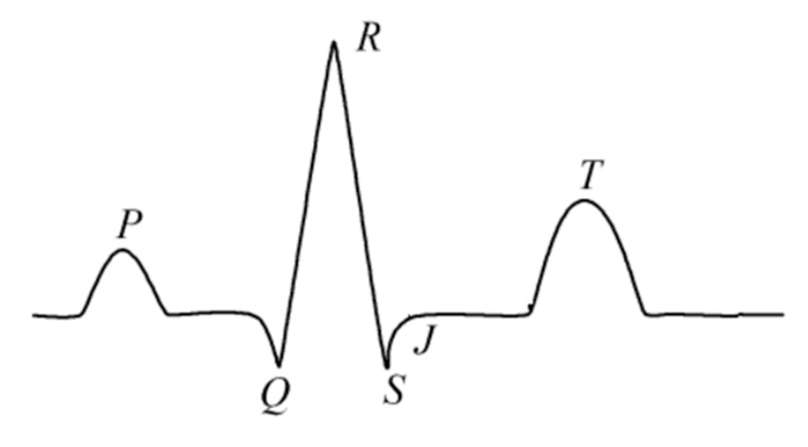
QRS detection is the basis for processing ECG signals [1]. Whatever function is ultimately implemented, the detection of QRS waves is a prerequisite, and the accurate detection of QRS waves (as shown in Figure 1) is therefore a prerequisite for feature extraction.
In a normal cardiac cycle, a typical ECG waveform is composed of a P wave, a QRS complex, a T wave and a U wave that may be seen in 50% to 75% of ECG [25]. The QRS complex [24] represents the rapid depolarization of the left and right ventricles. The ventricular muscles are larger compared to the atrium, so the amplitude of the QRS complex is usually much larger than that of the P wave [26], which indicates right atrial enlargement [6]. The baseline of the electrocardiogram is called the equipotential line. In general, the isopotential line in the ECG refers to the waveform after the T wave and before the P wave [24]. The Q, R and S waves occurring in rapid succession correspond to the depolarization of the left and right ventricles [27]; and the T wave [28] corresponds to the repolarization of the ventricles.
A four-layer wavelet transform based on a binary spline was used in this work. The R-wave can be detected by using the minimax method among the three-layer detail coefficients. The selection of the three-layer detail coefficient is based on the R-wave performance under the three-layer coefficient, which is different from other noises; the detailed implementation is presented next:
Binary Spline Wavelet Filter: Low Pass Filter: [1/4 3/4 3/4 1/4] and high-pass filter: [−1/4 −3/4 3/4 1/4].
First, find the minimum maximum pair in the layer 3 detail coefficient.
- Find the maximum value method: Find the position corresponding to a value of the slope >0, assign a value of 1, and the rest are 0. The maximum value is a sequence similar to 1, 0, that is, the position where the previous value is larger than the subsequent value or location point.
- Find the minimum value method: Find the position corresponding to the value of the slope <0, assign a value of 1, and the rest are 0. The minima are in positions corresponding to the sequence 1, 0, that is, the position where the previous value is lower than the later value.
- Set the threshold. The R-wave is extracted. The value of the R-wave is significantly larger than the value at other positions, and the characteristics of the detail coefficients at the three levels are similar. In this manner, a reliable threshold is set to extract a set of adjacent maximum and minimum pairs. (That is, divide all points into four parts. Find the average value T of the maximum value of each part. The threshold value is T/3). The zero crossing between the maximum and minimum is the R-wave point corresponding to the original signal.
- Compensate the R-wave point. In the process of the binary spline wavelet transform, there is a 10-point shift in the three-level detail coefficients and the corresponding position of the original signal; hence, compensation is required.
- Find the QS-wave. Based on the position of the R-wave, the first three poles at the position of the R-wave (under the layer 1 detail coefficient) are Q-waves. The last three poles at the position of the R-wave (with a detail coefficient of 1) are S-waves. Hence, the QRS-wave is detected.
In certain circumstances, the R-wave may be missed and misdetected; for example, the T-wave is detected as an R-wave. Hence, a missed detection and misdetection based on the distance of adjacent R-waves will be performed. This is a false detection when the distance of adjacent R-waves is <0.4 mean (RR) distance. This removes R-waves with small values. When the distance of adjacent R-waves is >1.6 mean (RR), find a maximum extremum pair between the two RR-waves and locate the R-wave. This is to prevent missed detections.
The above method developed a very robust QRS detection method. After testing, QRS detection reached 98%.
4.1.3. Feature Selection
Feature selection plays an important role in classification systems. Wavelet analysis was used by [6] for extracting features. The 12 features used in this experiment are (some of these are picked up from [6]):
- The average RR—interval duration.
- Standard deviation of RR—interval.
- GT50—the number of adjacent RR intervals, where the first RR interval exceeds the second RR interval by more than 50 milliseconds.
- LT50—the number of adjacent RR intervals whose second RR interval exceeds the first RR interval by more than 50 milliseconds.
- avgGT50, avgLT50—the above two variables (GT50 and LT50) are divided by the total number of RR intervals.
- SDSD—the standard deviation of the differences between adjacent RR intervals.
- The median of the RR interval.
- Interquartile range—the difference between the 75th and 25th percentiles of the RR interval value distribution.
- Mean Absolute Deviation—the average of the absolute values obtained by subtracting the average.
- RR interval value of all RR interval values in one period.
- Age of the observations.
- Sex of the observations.
4.2. SVM-Based Algorithm
This section presents both linear SVM and nonlinear SVM.
4.2.1. Linearly Separable SVM
When the data is linearly separable, this algorithm maximizes the hard interval, also known as hard interval SVM.
Input: Training dataset T = {(x1, y1), (x2, y2),…,(xn, yn)}, where xi belongs to Rn, yi belongs to {+1, −1}, i = 1,2,…n.
Output: Separating hyperplane and classification decision functions.
- Select the penalty parameter C > 0 to construct and solve the convex quadratic programming problem.Get the optimal solution .
- Calculate . Select a component of α* to meet the constraint:
- Find the separation hyperplane w*. x + b* = 0.
- Classification decision function: .
4.2.2. Linear SVM
When the data is approximately linearly divisible, the algorithm maximizes the soft interval, also known as soft interval SVM.
4.2.3. Nonlinear SVM
When the data is linearly inseparable, the algorithm uses kernel techniques to convert it into soft-spaced SVM.
A nonlinear classification problem can, in the input space, be transformed into a linear classification problem in a certain dimensional feature space through a nonlinear transformation, and a linear support vector machine is learned in a high-dimensional feature space. In the dual problem of linear support vector machine learning, both the objective function and the classification decision function only involve the inner product between the instances, so there is no need to explicitly specify the nonlinear transformation, but the kernel function is used to replace the inner product.
To construct SVMs, a kernel function has to be selected [1]. The kernel function represents the inner product between two instances after a nonlinear transformation.
Input: Training dataset T = {(x1, y1), (x2, y2),…,(xn, yn)}, where xi belongs to Rn, yi belongs to {+1, −1}, i = 1,2,…n.
Output: Separating hyperplane and classification decision functions.
Select the proper core function K(x, z) and the penalty parameter C > 0 to construct and solve the convex quadratic programming problem.
Get the optimal solution .
Select a component of α* to meet the constraint: , and then calculate .
Classification decision function:
The Gaussian kernel function is used:
The corresponding SVM is a Gaussian radial basis function (RBF) classifier. In this case, the classification decision function is:
Most practical applications have a high number of features. For example, in Chinese Optical character recognition, 8-direction gradient histogram features are extracted. The normalized characters are equally divided into 8 × 8 grids. Each grid calculates a direction histogram with a length of 8, so the feature dimension is 8 × 8 × 8 = 512 dimensions. In such high-dimensional space, it is easy to use linear SVM to separate two-character classes. The prediction function of linear SVM is f(x) = w ‘× x + b, and the classification speed is fast. For problems with many categories, the classification speed needs to take into account that the w of the linear classifier can be calculated in advance, while the number of support vectors for a nonlinear classifier in a high-dimensional space is very large, and the classification speed is much lower than the linear classifier. The generalization of linear SVM is guaranteed, while nonlinearity such as a Gaussian kernel may overfit. If the feature dimension is particularly low in the application scenario and the number of samples far exceeds the feature dimension, it is reasonable to choose a nonlinear kernel such as a Gaussian kernel. If the two classes have more overlap, the support vector of the nonlinear SVM is particularly large. Choosing a sparse nonlinear SVM will be a better solution, and the smaller the support vector is, the faster the classification will be.
5. The Dataset
For the experimentation, the database [29] from physionet was used, consisting of 70 records. Half the records were used for training the SVM classifier and half were used for testing. 35 records (a01 to a20, b01 to b05, c01 to c10) were used as the learning set, and 35 records (x01 to x35) were used as the test set. The length of all recorded recordings ranged from slightly less than 7 h to nearly 10 h. Each record consists of a continuous digitized ECG signal, a set of apnea notes (derived by experts based on the simultaneously recorded breath and related signals), and a set of machine-generated QRS annotations (in which all beats have been labelled as normal). In addition, there are eight records (a01 to a04, b01 and c01 to c03) through four additional signals (Resp C and Resp A, chest and abdominal respiratory effort signals obtained using inductive plethysmography; Resp N, nasal and nasal flow measured using a nasal thermistor; and SpO2, oxygen saturation).
6. Results and Analysis
The SVM model has two very important parameters, C and gamma. C is the penalty coefficient, the tolerance of error. A higher C indicates that the error cannot be tolerated and is easy to overfit. A lower C indicates that it can be easy to underfit. If C is too large or too small, generalization becomes a problem.
Gamma is a parameter that comes with the RBF function after it is selected as the kernel. The distribution of the data mapped to the new feature space is implicitly determined. The larger the gamma value, the smaller the support vector. The smaller the gamma value, the larger the support vector. The number of support vectors affects the speed of training and prediction.
The performances of the linear SVM, polynomial SVM and RBF SVM on the C and Gamma parameters were compared in the regular SVM framework as well as in the Big Data Spark-based SVM framework.
For the evaluation metrics, Accuracy, Sensitivity and Specificity were used.
Accuracy indicates the overall detection accuracy, determined by the formula:
Accuracy = ((TP + TN)/(TP + FP + TN + FN)) × 100%
Sensitivity is the ability of the classifier to accurately recognize OSA+, determined by the formula:
Sensitivity = (TP/TP + FN) × 100%
Finally, specificity indicates the classifier’s ability not to generate a false negative (normal subject, OSA−), determined by the formula:
Specificity = (TN/FP + TN) × 100%
Where TP is true positive, FP is false positive, FN is false negative and TN is true negative.
Table 1 presents the accuracy (%), sensitivity (%) and specificity (%) for C = 1 and 0.1 and Gamma = 0.1 and 0.2 for Linear SVM, Polynomial SVM and RBF SVM for regular SVM and SVM in the Big Data Framework in Spark.
The results show that the Spark-based kernel SVM with C = 1 and Gamma = 0.1 performed best, with an accuracy of 90.52% and specificity of 93.4%. With Gamma = 0.2, the accuracy was very close, at 90.35%. Polynomial Spark SVM also performed very well at C = 1, with an accuracy of 89.42% and specificity of 92.88%.
For C = 1, the polynomial SVM performed better than linear SVM in terms of accuracy, sensitivity, as well as specificity, for both regular SVM and Spark-SVM (it actually performed a lot better in Spark-SVM). For C = 0.1, the linear and polynomial SVM performed at almost the same level in terms of accuracy, but the polynomial SVM performed a lot better in terms of sensitivity and specificity, especially in Spark-SVM. This behavior of the C parameter is consistent, since for larger values of C a smaller margin is acceptable for classifying training points correctly, and for smaller values C a larger margin is acceptable for classifying training points correctly, hence compromising the accuracy.
When comparing the results of Gamma 0.1 and 0.2, overall, Gamma 0.1 performed better than Gamma 0.2. In most cases, the accuracy was very close, but the sensitivity and specificity were a little higher in most cases. Furthermore, overall, Spark-SVM performed better than regular SVM at Gamma 0.1. Again, this is consistent with the behavior of the Gamma parameter, since a lower Gamma parameter has a lower influence on the reach of the training sample, and a higher Gamma parameter has a higher influence on the reach of the training sample.
7. Conclusions
Wavelet decomposition and wavelet reshaping were used to denoise sleep apnea data, and cubic B-type interpolation wavelet transform was used to locate QRS complex numbers in OSA data. Twelve features were extracted and used for the prediction of OSA attacks, in regular SVM and Spark-SVM, with different configurations. From the results, it can be observed that Spark-SVM performed better than regular SVM, and C = 1 performed better that C = 0.1. Furthermore, Gamma 0.1 performed better than Gamma 0.2. One can also state that the polynomial SVM performed better than the linear SVM, both for regular SVM and Spark-SVM. Additionally, one can also state that, overall, in terms of accuracy and specificity, Spark-SVM performed better than regular SVM. Spark-SVM also performed better than regular SVM in terms of time/speed. This was predictable, since Spark-SVM uses a distributed and parallelized environment. In comparison to previous SVM-based models, this work, in using this set of 12 features, performs better than [21] in terms of accuracy and performs comparably to [1,18,22].
8. Future Work
There is a lot of scope for more work to be done with Spark SVM in the big data environment. The effect of varying the number of cores on the timings of Spark’s SVM could be studied in detail for the linear, polynomial, as well as RBF SVM using various C and Gamma parameters. Other optimization features of Spark can also be used to finetune and optimize the results.
Author Contributions
This project was conceptualized by S.B. and K.J., K.J. did most of the programming. The paper was composed by both S.B. and K.J. All authors have read and agreed to the published version of the manuscript.
Funding
This research received no external funding.
Acknowledgments
This work has been partially supported by the Askew Institute of the University of West Florida.
Conflicts of Interest
The authors declare no conflict of interest.
References
- Khandoker, A.H.; Palaniswami, M.; Karmakar, C.K. Support Vector Machines for Automated Recognition of Obstructive Sleep Apnea Syndrome from ECG Recordings. IEEE Trans. Inf. Technol. Biomed. 2009, 13, 37–47. [Google Scholar] [CrossRef] [PubMed]
- Coleman, J. Complications of Snoring, Upper Airway Resistance Syndrome, and Obstructive Sleep Apnea Syndrome in Adults. Otolaryngol. Clin. North Amer. 1999, 32, 223–234. [Google Scholar] [CrossRef]
- Vgontzas, A.N.; Papanicolaou, D.A.; Bixler, E.O.; Hopper, K.; Lotsikas, A.; Lin, H.M.; Kales, A.; Chrousos, G.P. Sleep Apnea and Daytime Sleepiness and Fatigue: Relation to Visceral Obesity, Insulin Resistance, and Hypercytokinemia. J. Clin. Endocrinol. Metab. 2002, 85, 1151–1158. [Google Scholar] [CrossRef] [PubMed]
- Young, T.; Palta, M.; Dempsey, J.; Peppard, P.E.; Nieto, F.J.; Hla, K.M. Burden of Sleep Apnea: Rationale, Design, and Major Findings of the Wisconsin Sleep Cohort Study. WMJ 2009, 108, 246–249. [Google Scholar]
- Gibson, G.J. Obstructive Sleep Apnoea Syndrome: Underestimated and Undertreated. Br. Med Bull. 2004, 72, 49–65. [Google Scholar] [CrossRef] [PubMed]
- Almazaydeh, L.; Elleithy, K.; Faezipour, M. Obstructive Sleep Apnea Detection Using SVM-Based Classification of ECG Signal Features. In Proceedings of the 34th Annual International Conference of the IEEE EMBS, San Diego, CA, USA, 28 August–1 September 2012; pp. 4938–4941. [Google Scholar]
- Common Signs of Sleep Apnea. Available online: https://www.nhlbi.nih.gov/health-topics/sleep-apnea (accessed on 18 July 2020).
- Golbidi, S.; Badran, M.; Ayas, N.; Laher, I. Cardiovascular Consequences of Sleep Apnea. Lung 2012, 190, 113–132. [Google Scholar] [CrossRef] [PubMed]
- Dimsdale, J.E.; Loredo, J.S.; Profant, J. Effect of Continuous Airway Pressure on Blood Pressure. Hypertension 2000, 35, 144–147. [Google Scholar] [CrossRef] [PubMed]
- Canessa, N.; Castronovo, V.; Cappa, S.F.; Aloia, M.S.; Marelli, S.; Falini, A.; Alemanno, F.; Ferini-Strambi, L. Obstructive Sleep Apnea: Brain Structural Changes and Neurocognitive Function Before and After Treatment. Am. J. Respir. Crit. Care Med. 2011, 183, 1419–1426. [Google Scholar] [CrossRef] [PubMed]
- Young, T.; Peppard, P.E.; Gottlieb, D.J. Epidemiology of Obstructive Sleep Apnea: A Population Health Perspective. Am. J. Respir. Crit. Care Med. 2002, 165, 1217–1239. [Google Scholar] [CrossRef]
- Yaggi, H.K.; Concato, J.; Kernan, W.N.; Lichtman, J.H.; Brass, L.M.; Mohsenin, V. Obstructive Sleep Apnea as a Risk Factor for Stroke and Death. N. Engl. J. Med. 2005, 353, 2034–2041. [Google Scholar] [CrossRef] [Green Version]
- Manoochehri, Z.; Salari, N.; Rezael, M.; Khazaie, H.; Manoochehri, S.; Pavah, B.K. Comparison of Support Vector Machine Based on Genetic Algorithm with Logistic Regression to Diagnose Obstructive Sleep Apnea. J. Res. Med Sci. 2018, 23, 1–14. [Google Scholar] [CrossRef]
- Le, T.Q. A Nonlinear Stochastic Dynamic Systems Approach for Personalized Prognostis of Cardiorespiratory Disorders. Ph.D. Thesis, Oklahoma State University, Stillwater, OK, USA, 2013. [Google Scholar]
- Le, T.Q.; Cheng, C.; Sangasoongsong, A.; Wongdhamma, W.; Bukkapatnam, S.T. Wireless wearable multisensory suite and real-time prediction of obstructive sleep apnea episodes. IEEE J. Transl. Eng. Health Med. 2013, 1, 2700109. [Google Scholar] [CrossRef] [PubMed]
- Le, T.Q.; Bukkapatnam, S.T. Nonlinear dynamics forecasting of obstructive sleep apnea onsets. PLoS ONE 2016, 11, e0164406. [Google Scholar] [CrossRef] [Green Version]
- Ramírez-Gallego, S.; Krawczyk, B.; García, S.; Woźniak, M.; Benítez, J.M.; Herrera, F. Nearest neighbor classification for high-speed big data streams using spark. IEEE Trans. Syst. Manand Cybern. Syst. 2017, 47, 2727–2739. [Google Scholar] [CrossRef]
- Shao, S.; Wang, T.; Song, C.; Chen, X.; Cui, E.; Zhao, H. Obstructive Sleep Apnea Recognition Based on Multi-Bands Spectral Entropy Analysis of Short-Time Heart Rate Variability. Entropy 2019, 21, 812. [Google Scholar] [CrossRef] [Green Version]
- Vladimir, N.V. Statistical Learning; Wiley: Hoboken, NJ, USA, 1998. [Google Scholar]
- Guller, M. Big Data Analysis with Spark; Apress: New York, NY, USA, 2015. [Google Scholar]
- Al-Angari, H.M.; Sahakian, A.V. Automated Recognition of Obstructive Sleep Apnea Syndrome Using Support Vector Machine Classifier. IEEE Trans. Inf. Technol. Biomed. 2012, 16, 463–468. [Google Scholar] [CrossRef] [PubMed] [Green Version]
- Maali, Y.; Al-Jumaily, A.; Laks, L. Self-Advising SVM for Sleep Apnea Classification. 2012. Available online: https://www.semanticscholar.org/paper/Self-advising-SVM-for-sleep-apnea-classification-Maali-Al-Jumaily/a833ab4f2f10a3b7b87919d0df65ddaed8a12160 (accessed on 21 September 2020).
- Liu, W.-L.; Wu, H.-T.; Juang, J.-N.; Wisniewski, A.; Lee, H.-C.; Wu, D.; Lo, Y.-L. Prediction of the severity of obstructive sleep apnea by anthropometric features via support vector machine. PLoS ONE 2017, 12, e0176991. [Google Scholar] [CrossRef] [PubMed] [Green Version]
- Electrocardiography. Available online: https://en.wikipedia.org/wiki/Electrocardiography (accessed on 18 November 2019).
- “Limb Leads—ECG Lead Placement—Normal Function of the Heart—Cardiology Teaching Package—Practice Learning—Division of Nursing—The University of Nottingham”. Nottingham.ac.uk. Available online: https://www.nottingham.ac.uk/nursing/practice/resources/cardiology/function/limb_leads.php (accessed on 15 August 2019).
- P Wave_(electrocardiography). Available online: https://en.wikipedia.org/wiki/P_wave_(electrocardiography) (accessed on 18 July 2020).
- QRS Complex. Available online: https://en.wikipedia.org/wiki/QRS_complex (accessed on 18 July 2020).
- T Wave. Available online: https://en.wikipedia.org/wiki/T_wave (accessed on 18 July 2020).
- Goldberger, A.L.; Amaral, L.A.N.; Glass, L.; Hausdorff, J.M.; Ivanov, P.C.; Mark, R.G.; Mietus, J.E.; Moody, G.B.; Peng, C.-K.; Stanley, H.E. PhysioBank, PhysioToolkit, and PhysioNet: Components of a New Research Resource for Complex Physiologic Signals. Circulation 2003, 101, e215–e220. [Google Scholar] [CrossRef] [PubMed] [Green Version]
Figure 1.
Wave form of QRS complex.


Table 1.
Performance comparison of SVMs.
| C | Gamma | Accuracy (%) | Sensitivity (%) | Specificity (%) | ||
|---|---|---|---|---|---|---|
| Regular SVM | Linear | 1 | 86.16 | 89.64 | 83.51 | |
| Polynomial | 1 | 87.6 | 93.36 | 83.22 | ||
| RBF | 1 | 0.1 | 88.86 | 93.2 | 87.66 | |
| RBF | 1 | 0.2 | 87.46 | 91.67 | 80.52 | |
| Spark-SVM | Linear | 1 | 85.72 | 82.25 | 91.4 | |
| Polynomial | 1 | 89.42 | 85.67 | 92.88 | ||
| RBF | 1 | 0.1 | 90.52 | 86.1 | 93.4 | |
| RBF | 1 | 0.2 | 90.35 | 84.79 | 86.2 | |
| Regular SVM | Linear | 0.1 | 82.2 | 40.2 | 91.1 | |
| Polynomial | 0.1 | 84.1 | 56.8 | 87.1 | ||
| RBF | 0.1 | 0.1 | 83.82 | 53.08 | 84.35 | |
| RBF | 0.1 | 0.2 | 81.58 | 52.8 | 78.82 | |
| Spark-SVM | Linear | 0.1 | 83.6 | 48.5 | 81.8 | |
| Polynomial | 0.1 | 84.1 | 61.6 | 92.88 | ||
| RBF | 0.1 | 0.1 | 85.5 | 81.68 | 91.48 | |
| RBF | 0.1 | 0.2 | 85.15 | 79.35 | 86.96 |
© 2020 by the authors. Licensee MDPI, Basel, Switzerland. This article is an open access article distributed under the terms and conditions of the Creative Commons Attribution (CC BY) license (http://creativecommons.org/licenses/by/4.0/).
Share and Cite
MDPI and ACS Style
Jin, K.; Bagui, S. Apache Spark SVM for Predicting Obstructive Sleep Apnea. Big Data Cogn. Comput. 2020, 4, 25. https://0-doi-org.brum.beds.ac.uk/10.3390/bdcc4040025
AMA Style
Jin K, Bagui S. Apache Spark SVM for Predicting Obstructive Sleep Apnea. Big Data and Cognitive Computing. 2020; 4(4):25. https://0-doi-org.brum.beds.ac.uk/10.3390/bdcc4040025
Chicago/Turabian StyleJin, Katie, and Sikha Bagui. 2020. "Apache Spark SVM for Predicting Obstructive Sleep Apnea" Big Data and Cognitive Computing 4, no. 4: 25. https://0-doi-org.brum.beds.ac.uk/10.3390/bdcc4040025