Article

Robust Multi-Mode Synchronization of Chaotic Fractional Order Systems in the Presence of Disturbance, Time Delay and Uncertainty with Application in Secure Communications

by
Ali Akbar Kekha Javan
1,
Assef Zare
1,*,
Roohallah Alizadehsani
2 and
Saeed Balochian
1
1
Department of Electrical Engineering, Gonabad Branch, Islamic Azad University, Gonabad 6518115743, Iran
2
Institute for Intelligent Systems Research and Innovation (I.I.S.R.I.), Deakin University, Geelong, VIC 3216, Australia
*
Author to whom correspondence should be addressed.
Big Data Cogn. Comput. 2022, 6(2), 51; https://0-doi-org.brum.beds.ac.uk/10.3390/bdcc6020051
Submission received: 12 April 2022 / Revised: 28 April 2022 / Accepted: 29 April 2022 / Published: 8 May 2022

Abstract

:
This paper investigates the robust adaptive synchronization of multi-mode fractional-order chaotic systems (MMFOCS). To that end, synchronization was performed with unknown parameters, unknown time delays, the presence of disturbance, and uncertainty with the unknown boundary. The convergence of the synchronization error to zero was guaranteed using the Lyapunov function. Additionally, the control rules were extracted as explicit continuous functions. An image encryption approach was proposed based on maps with time-dependent coding for secure communication. The simulations indicated the effectiveness of the proposed design regarding the suitability of the parameters, the convergence of errors, and robustness. Subsequently, the presented method was applied to fractional-order Chen systems and was encrypted using the chaotic masking of different benchmark images. The results indicated the desirable performance of the proposed method in encrypting the benchmark images.

1. Introduction

Today, many people use digital communications in daily activities, changing this field into one of the most special human needs [1,2,3]. Additionally, digital communications facilitate commerce in different industrial and medical contexts [4,5]. In that regard, information security is vital. The digital communications system includes a transmitter, communication channel, and receiver. Information security in communication channels is of great importance. The particular importance of information security in digital communications has led to extensive studies in this domain, and scientists have presented various methods [6,7,8,9]. Encryption is one of the most important information security contexts in digital communications and includes multiple methods such as chaos theory techniques [10]. Numerous synchronization techniques for various chaotic systems have been proposed based on control techniques. Generally, chaotic systems fall into standard and fractional order types, and each is analyzed in many synchronization systems. Control methods applied in synchronization incorporate linear and nonlinear [11,12], fuzzy [13], active [14,15], backstepping [16,17], sliding mode control (SMC) [18,19], and adaptive control [20]. Lai used various methods such as designing a new memristor that is flux-controlled [21], a Lü chaos system with coexisting attractors and a nonlinear controller [22], and a new encryption algorithm performed on hyper chaotic neurons [23] to enhance image encryption security.
The idea of this paper is to employ SMC alongside three chaotic systems. To further increase efficiency, the parameters of the chaotic systems that are unknown are introduced. The authors in [24] investigated Hopf bifurcation and amplitude controls in the chaotic Toda jerk oscillator system with analysis, circuit realization, and combined synchronization in the fractional-order form. In [25], the multi-switching synchronization of several chaotic systems was examined. The proposed Lorenz and Chen chaotic systems were adopted and explained three-dimensionally. However, in relevant studies, it has been assumed that their parameters are known. In [26], the combination synchronization of a new fractional-order chaotic system with two stable node-foci was studied. In [27], dual-phase and dual anti-phase synchronization of FOCS in real and complex variables with uncertainties was investigated. The effect of disturbance is not considered in this paper. The authors in [28] studied the combination synchronization of three fractional-order time-delayed chaotic systems without disturbance and uncertainty. The authors in [29] surveyed multi-switching combination-combination synchronization of unknown FOCS, in which three-dimensional systems were exploited, and the effect of disturbance was not studied. Various studies deal with system synchronization applications in secure communication: Khan and Nigar (2020) used sliding-mode disturbance observer control based on adaptive hybrid projective combination synchronization in fractional-order systems [30]. An adaptive-robust control for multi-state synchronization of chaotic systems with unknown and time-varying delay was studied by Kekha javan [31].
A chaotic system with an exponential term was considered in [32] to study its synchronization. It seeks the dynamics of approximation of exponential chaotic systems. Moreover, combination synchronization was used to control this system. Afterward, its application was exhibited in secure communication. An application of uncertain chaotic system adaptive synchronization was studied in secure communication systems in [33]. Khan et al., (2019) proposed a secure communication design through novel fractional chaotic system synchronization [34]. A finite-time terminal auxiliary observer was used for fractional-order chaotic systems with application in secure communication [35]. The authors in [36] used secure communication via projective synchronization of the fractional matrix. In [37], a secure communication design was used based on the modified hybrid projective synchronization of fractional hyper-chaotic systems. A novel acoustic encryption method with finite-time synchronization of the fractional-order hyper-chaotic system was proposed [38]. Vaseghi et al. (2021) applied finite-time synchronization in chaotic systems to encrypt medical images [39].
Previous research indicates the gap regarding the multi-mode synchronization of fractional-order hyper-chaotic systems with unknown and variable parameters using an adaptive-robust controller. Accordingly, this paper aims to demonstrate a multi-mode synchronization scheme for fractional-order hyper-chaotic systems with parametric uncertainty and disturbances. The boundaries of these uncertainties and disturbances are estimated by applying adaptive rules. Furthermore, its detrimental effect on the performance of synchronization control law is significantly reduced. The proposed novel secure communication method uses chaotic masking with a new modulation function for benchmark image encryption. Information entropy, signal-to-noise ratio, histogram, and similar criteria were used to analyze the proposed method.
The main contributions of the present study are as follows:
(1)
Synchronization, despite the stepwise changes of system parameters.
(2)
Determination of control rule as an explicit and continuous function that prohibits the manifestation of chattering phenomenon.
(3)
Synchronization is independent of the type of chaotic system.
(4)
Determination of several adaptive rules such that the system stability is guaranteed and the convergence of synchronization errors and estimating errors of disturbance and uncertainty boundaries converge to zero.
(5)
A novel secure communication design was considered the modulation function for chaotic masking.
To evaluate the performance of the proposed scheme, simulations were carried out on three fractional-order hyper-chaotic Chen systems with unknown parameters and external disturbances. Their results indicated the adequacy and robustness of the proposed adaptive controller scheme.
The next part of this paper presents the formulation of the proposed method. It contains the fractional-order systems and adaptive synchronization of multiple FOCS with unknown parameters expressed in two transmission and circular multi-mode synchronization. This issue was also tested in the presence of disturbance. Section 4 presents the simulation results. The standard benchmark images were simulated and evaluated with the statistic criterion. The efficiency of the method was evaluated by histogram analysis, correlation analysis, number of pixel change rate (NPCR), unified average changing intensity (UACI), peak signal to noise ratio (PSNR), and information entropy. The experiment results indicated the proposed encryption method’s ability to uplift security and performance. Section 6 presents the discussion of the proposed method, followed by the conclusion.

2. Problem Formulation

This section discusses the proposed scheme of the paper. First, fractional-order systems are presented. Subsequently, the synchronization of chaotic systems of multiple transmission fractional order is described. Finally, the multiple circular synchronizations are discussed. In both cases, adaptive rules and controllers are designed using the adaptive control method. Two examples are given to demonstrate the efficiency and performance of the proposed method.

2.1. Basic Definitions

Fractional-Order Derivative

Due to simple implementation and high performance, several numerical definitions have been proposed to solve fractional differential equations [40]. This paper uses the definition of Caputo, whose fractional derivative is as follows [40]:
D q f ( x ) = I m q h ( m ) ( x ) ,   q > 0
where h ( m ) represents the derivative of mth order of h(x), m = [q] is the first integer that is less than q, and the Riemann-Lewil integral operator with order q of function g(x) is described as follows [40]:
I q g ( x ) = 1 Γ ( q ) 0 x ( x t ) q 1 g ( t ) d t ,   q > 0
where Γ ( q ) is the gamma function and the D q operator is called the Caputo fractional operator of q order.
Stability analysis of fractional-order systems by Lyapunov’s direct method and determining the necessary and sufficient conditions guaranteeing stability with the Mittag-Leffler concept [41] and stability analysis based on convex of the Lyapunov functions [40] for nonlinear systems are demonstrated.
Lemma 1.
[40]: Suppose h ( t ) R is a continuous and derivable function. Then, for t t 0 , we have:
D q h 2 ( t ) 2 h ( t ) · D q h ( t )
Lemma 2.
[40]: Suppose h ( t ) R n is a continuous and derivable function. Then, for t t 0 , we have:
D q h T ( t ) h ( t ) 2 h T ( t ) · D q h ( t )
Theorem 1.
[41]: Suppose x = 0 is the equilibrium point of the fractional-order system (5) and its definition domain includes the origin. Suppose V ( t . x ( t ) ) is continuous and derivable and that the Lipschitz function is relative to x such that:
D q x ( t ) = f ( x . t )
a 1 x a V ( t . x ( t ) ) a 2 x a b
D q V ( t . x ( t ) ) a 3 x a b
where 0 < q < 1 and a 1 ,   a 2 ,   a 3 ,   a ,   b are arbitrary and positive constants. Then, x = 0 is stable in the sense of Mittag-Leffler.
Definition 1.
The continuous function p : [ 0 , ) [ 0 , ) belongs to the class-K if it is strictly increasing and p ( 0 ) = 0 .
Theorem 2.
[41]: Suppose x = 0 is the equilibrium point of the fractional-order system (5), where f ( x . t ) satisfies the Lipshitz condition and q ( 0 , 1 ) . If the relations (8) and (9) are established for the Lyapunov function V(t,x(t)) and the class-K functions δ i :
δ 1 ( x ) V ( t . x ( t ) ) δ 2 ( x )
D q V ( t . x ( t ) ) δ 3 ( x )
Then, the system (5) is asymptotically stable in the sense of Mittag-Leffler [42].
Theorem 3.
[43]: For the fractional-order system (5) and the Lyapunov function V ( x ) :
D q V ( x ) ( V x ) T · D q x = ( V x ) T · f ( x . t )

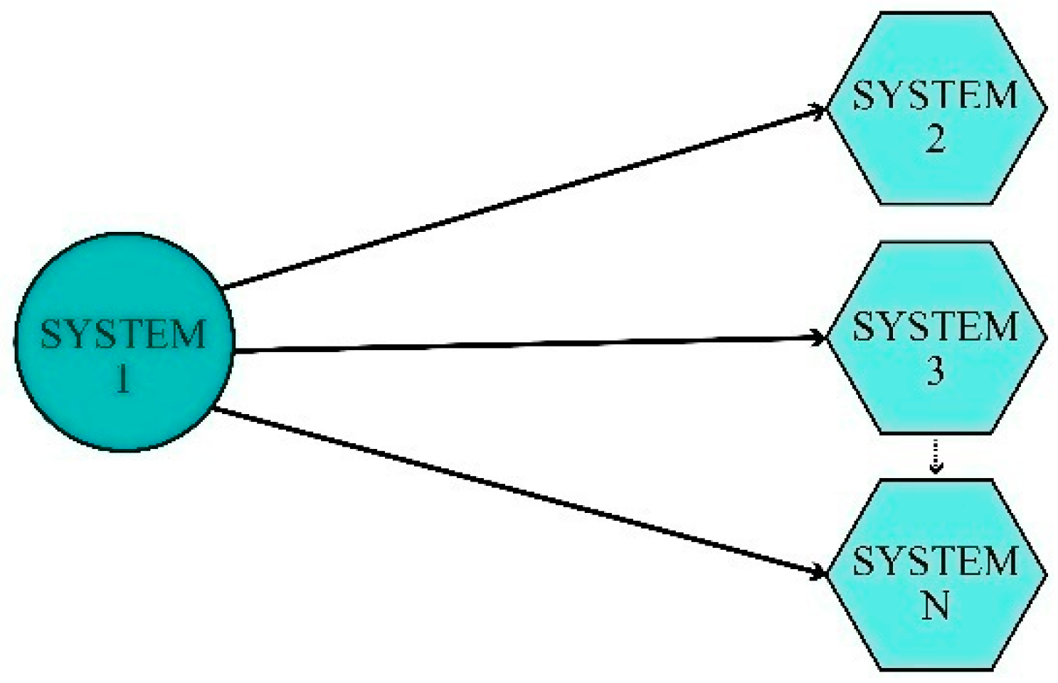
2.2. Adaptive Synchronization between One Drive System and Several Response Systems

Figure 1 shows the synchronization between one master system and several slave systems.
The master hyper-chaotic system with unknown parameters is as follows [44]:
D q x 1 ( t ) = f 1 ( x 1 ) + H 1 ( x 1 ) θ 1 ( t )
where x 1 ( t ) = [ x 11 , x 12 , , x 1 n ] T are the state vectors of the system, f 1 ( x 1 ( t ) ) = [ f 11 , f 12 , , f 1 n ] T is a continuous function, H 1 ( x 1 ( t ) ) = [ H 11 , H 12 , , H 1 n ] T is the matrix function, and θ 1 ( t ) = [ θ 11 , θ 12 . . θ 1 n ] T are the basic parameters of the master system that are unknown and variable.
N-1 slave hyper-chaotic systems with control function are as follows [44]:
D q x i ( t ) = f i ( x i ) + H i ( x i ) θ i ( t ) + u i 1 ( t )               i = 2 , 3 , , N
where x i ( t ) = [ x i 1 , x i 2 , , x i n ] T is the state vector of ith system, f i ( x 1 ( t ) ) = [ f i 1 , f i 2 , , f i n ] T is the continuous function, H i ( x i ( t ) ) = [ H i 1 , H i 2 , , H i n ] T is the matrix function, θ i ( t ) = [ θ i 1 , θ i 2 , , θ i n ] T are the basic parameters of ith slave system, and u i 1 ( t ) = [ u i 1.1 ( t ) , u i 1.2 ( t ) , , u i 1 . n ( t ) ] T is the control function of ith slave system. Therefore, according to Equations (11) and (12), the synchronization of the chaotic system with the control function is stated as follows:
{ D q x 1 ( t ) = f 1 ( x 1 ) + H 1 ( x 1 ) θ 1 D q x 2 ( t ) = f 2 ( x 2 ) + H 2 ( x 2 ) θ 2 + u 1 ( t ) D q x N ( t ) = f N ( x N ) + H N ( x N ) θ N + u N 1 ( t )
In multimode synchronization form, the synchronization error is given as follows:
e i 1 ( t ) = x i ( t ) x 1 ( t )   i = 2 , 3 , , N
Definition 2.
For N FOCS expressed by (13), if adaptive controllers u i 1 ( t ) exist such that for dynamic systems the error is given by:
D q e i 1 ( t ) = f i ( x i ) f 1 ( x 1 ) + H i ( x i ) θ i H 1 ( x 1 ) θ 1 + u i 1 ( t )                 i = 2 , 3 ,   , N 1
The required conditions are:
lim t e i 1 ( t ) = lim t x i ( t ) x 1 ( t ) 0     i = 2 , 3 , , N
If satisfied, then the adaptive transmission multi-mode synchronization between N chaotic systems with unknown parameters is realized. The design of controllers and adaptive rules to achieve the above objective is based on the Lyapunov function, and synchronization is fulfilled with transmission mode synchronization. The controller law for u 1 ( t ) , u 2 ( t ) , u 3 ( t ) , , u N 1 ( t ) is designed as below:
u i 1 ( t ) = f i ( x i ) + f 1 ( x 1 ) H i ( x i ) θ ^ i + H 1 ( x 1 ) θ ^ 1 + K i 1 e i 1     i = 2 , 3 , , N 1
Therefore, the errors of dynamics are given as follows:
D q e i 1 ( t ) = H i ( x i ) θ ˜ i H 1 ( x 1 ) θ ˜ 1 + K i 1 e i 1     i = 2 , 3 , , N 1
where θ ^ i is the estimation of θ i , θ ˜ i ( t ) = θ i ( t ) θ ^ i ( t ) is an approximation error, and:
K i 1 = d i a g ( k i 1 , 1 . k i 1 , 2 . . k i 1 , n ) .   k i 1 , j < 0   j = 1 , 2 , , n

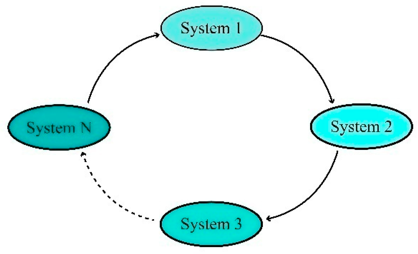
2.3. Adaptive Circular Multimode Synchronization of Chaotic Systems

Figure 2 depicts a demonstration of circular multi-mode synchronizations. In this type of synchronization, all systems (except system 1) play both slave and master roles contemporarily, which helps to achieve more complexity.
In this case, the first chaotic system is described as the following.
D q x 1 ( t ) = f 1 ( x 1 ) + H 1 ( x 1 ) θ 1
The N-1 chaotic systems are given as follows [44]:
{ D q x 1 ( t ) = f 1 ( x 1 ) + H 1 ( x 1 ) θ 1 D q x 2 ( t ) = f 2 ( x 2 ) + H 2 ( x 2 ) θ 2 + m 1 ( t ) D q x N ( t ) = f N ( x N ) + H N ( x N ) θ N + m N 1 ( t )
Control input is in the form of m i 1 ( t ) = [ m i 1.1 . m i 1.2 . . m i 1 . n ] T .
For N chaotic system explained by (18), if there are adaptive controllers such that the error dynamic systems are given as follows:
r i ( t ) = x i + 1 ( t ) x i ( t ) i = 1 , 2 , 3 , N 1  
D q r i 1 ( t ) = f i ( x i ) f i 1 ( x i 1 ) + H i ( x i ) θ i H i 1 ( x i 1 ) θ i 1 + m i 1 m i 2 i = 2 , 3 , , N 1
In addition, conditions are given by:
lim t r i 1 ( t ) = lim t x i ( t ) x i 1 ( t ) 0               i = 2 , 3 , , N
If satisfied, then an adaptive circular multi-mode synchronization between N chaotic systems with unknown parameters is accomplished.
Theorem 4.
For multi-mode synchronization of hyper-chaotic in two circular and transitional states, the following statements are satisfied.
1-A. If the transmission and circular synchronization are established with the controllers u i ( t ) and m i ( t ) , then:
i . j   :     lim t x i ( t ) x j ( t ) 0
2-A. If transmission synchronization is established, then circular synchronization is also realized and vice versa.
Proof 1-A.
Suppose there is a transmission synchronization, therefore:   i   :   e i ( t ) 0 . Thus:
i . j : x i ( t ) x j ( t ) = ( x i ( t ) x 1 ( t ) ) ( x j ( t ) x 1 ( t ) ) e i ( t ) + e j ( t ) 0
If circular synchronization is met (assuming i > j):
i . j : x i ( t ) x j ( t ) = ( x i ( t ) x i 1 ( t ) ) + ( x i 1 ( t ) x i 2 ( t ) ) + + ( x j + 1 ( t ) x j ( t ) ) r i 1 ( t ) + + r j ( t ) = k = j i 1 r k ( t ) 0  
Proof 2-A.
The following relationships between errors exist in two synchronization modes:
r i ( t ) = { e i ( t ) e i 1 ( t )           i = 2 , 3 , , N 1   e i ( t )                 i = 1   .   e i ( t ) = k = 1 i r k ( t )
If the transmission synchronization is true, e i ( t ) 0 ; therefore:
r i ( t ) = { e i ( t ) e i 1 ( t ) e i ( t ) + e i 1 ( t ) 0 i 2 e 1 ( t ) 0 i = 1
So, circular synchronization is true.
Conversely, assume that circular synchronization is true; r i ( t ) 0 . Therefore:
e i ( t ) = k = 1 i r k ( t ) k = 1 i r k ( t ) 0
Therefore, transmission synchronization is also true. So, both types of synchronization are equivalent to each other.
Theorem 5.
The control law is identical for transmission synchronization u i ( t ) and circular synchronization m i ( t ) of the fractional-order of chaotic systems.
Proof. 
Utilizing the relationship between two types of errors, we have:
D q e i ( t ) = D q e i 1 ( t ) + D q r i ( t )
Which can be acquired by substituting in Equations (14) and (23):
u i 1 ( t ) = u i ( t ) ( m i ( t ) m i 1 ( t ) )   i 2
For i = 1, we have:
e 1 ( t ) = r 1 ( t ) D q e 1 ( t ) = D q r 1 ( t ) m 1 ( t ) = u 1 ( t )
By the substitution of (22) in (21) we have: m i ( t ) = u i ( t ) ; hence, the proof is complete.

2.4. Synchronization in the Presence of Disturbance, Time Delay and Uncertainty in the Systems

In this case, the master and slave system with disturbance, time delay, and uncertainty is as follows:
D q x 1 t = f 1 x 1 + H 1 x 1 θ 1 + + F 1 x 1 t τ 1 + Δ f 1 x 1 + D 1 t D q x 2 t = f 2 x 2 + H 2 x 2 θ 2 + F 2 x 2 t τ 2 + Δ f 2 x 2 + D 2 t + u 1 t D q x N t = f N x N + H N x N θ N + F N x N t τ N + Δ f N x N + D N t + u N 1 t
It is assumed that   F i ( x i ( t τ i ) ) are Lipschitz, uncertainties and disturbances are bounded but with an unknown boundary.
| Δ f i ( x i ) | γ i g i ( x i )   .                 | D i ( t ) | d i     i = 1 , 2 , , N
| F i ( x i ( t τ i ) ) F i ( x i ( t p i ) ) | l i | τ i p i |
where γ i ,   l i and d i are constant but unknown and g i ( x i ) is definite and positive. The error dynamic is described as follows:
D q e i 1 ( t ) = f i ( x i ) f 1 ( x 1 ) + H i ( x i ) θ i H 1 ( x 1 ) θ 1 + F i ( x i ( t τ i ) ) F 1 ( x 1 ( t τ 1 ) ) + Δ f i ( x i ) Δ f 1 ( x 1 ) + D i ( t ) D 1 ( t ) + u i 1 ( t )                 i = 2 , 3 , , N 1
Defining the control function as follows:
u i 1 ( t ) = f i ( x i ) + f 1 ( x 1 ) H i ( x i ) θ ^ i + H 1 ( x 1 ) θ ^ 1 + K i 1 e i 1 F i ( x i ( t τ ^ i ) ) + F 1 ( x 1 ( t τ ^ 1 ) ) + u ¯ i 1 ( t ) i = 2 , 3 , , N 1
where θ ^ i , τ ^ i are estimations of θ i ,   τ i and u ¯ i 1 ( t ) is the section of the control function, which is introduced below. By placing the control function in (24), the error dynamics are given as follows:
D q e i 1 ( t ) = H i ( x i ) θ ˜ i H 1 ( x 1 ) θ ˜ 1 + Δ f i ( x i ) Δ f 1 ( x 1 ) + D i ( t ) D 1 ( t ) + K i 1 e i 1 + F i ( x i ( t τ i ) ) F 1 ( x 1 ( t τ 1 ) ) F i ( x i ( t τ ^ i ) ) + F 1 ( x 1 ( t τ ^ 1 ) ) + u ¯ i 1 ( t ) ,     i = 2 , 3 , , N 1
Theorem 6.
The error dynamics system (26) is under control law (36), the update rules (35) are stable, and the synchronization errors converge to zero despite the uncertainty, time delay, and disturbance.
Proof. 
By explaining the Lyapunov function as follows:
V = 1 2 ( V e + V θ + V γ + V d + V τ )  
Wherein:
V e = i = 2 N e i 1 T K i 1 e i 1 V θ = i = 2 N θ ˜ i T θ ˜ i + θ ˜ 1 T θ ˜ 1
V γ = i = 2 N γ ˜ i 2 + γ ˜ 1 2   ,   V d = i = 2 N d ˜ i 2 + d ˜ 1 2   , V τ = i = 2 N l i τ ˜ i 2 + l 1 τ ˜ 1 2
and: θ ˜ i = θ i θ ^ i ,   γ ˜ i = γ i γ ^ i ,   d ˜ i = d i d ^ i ,   τ ˜ i = τ i τ ^ i .
By calculating the fractional derivative of the Lyapunov function and replacing control function (27):
D q V i = 2 N [ e i 1 T ( H i x i θ ˜ i H 1 x 1 θ ˜ 1 + Δ f i x i Δ f 1 x 1 + F i x i t τ i F i x i t τ ^ i F 1 x 1 t τ 1                                                         + F 1 x 1 t τ ^ 1 + D i t D 1 t + 1 2 K i 1 + K i 1 T e i 1 ) + θ ˜ i T D q θ ˜ i + γ ˜ i D q γ ˜ i + d ˜ i D q d ˜ i + l i τ ˜ i D q τ i                                                         + u ¯ i 1 t ] + θ ˜ 1 T D q θ ˜ 1 + γ ˜ 1 D q γ ˜ 1 + d ˜ 1 D q d ˜ 1 + l 1 τ ˜ 1 D q τ 1
If u ¯ i j ,   Δ f i j ,   D i j ,   e i 1 j is the component jth of the vectors u ¯ i 1 ( t ) ,   Δ f i ,   D i ,   e i 1 , respectively. Then:
D q V i = 2 N j = 1 n e i 1 j ( Δ f i j Δ f 1 j + D i j D 1 j + F i x i t τ i F i x i t τ ^ i F 1 x 1 t τ 1 + F 1 x 1 t τ ^ 1                                                         + u ¯ i 1 j ) + i = 2 N [ e i 1 T H i x i θ ˜ i H 1 x 1 θ ˜ 1 + θ ˜ i T D q θ ˜ i ] + i = 2 N γ ˜ i D q γ ˜ i + d ˜ i D q d ˜ i + l i τ ˜ i D q τ i                                                         + i = 2 N 1 2 e i 1 T K i 1   +   K i 1 T e i 1 + γ ˜ 1 D q γ ˜ 1 + d ˜ 1 D q d ˜ 1 + l 1 τ ˜ 1 D q τ 1 + θ ˜ 1 T D q θ ˜ 1
Therefore:
D q V i = 2 N j = 1 n [ e i 1 j Δ f i j + Δ f 1 j + D i j + D 1 j + F i x i t τ i F i x i t τ ^ i + F 1 x 1 t τ 1 + F 1 x 1 t τ ^ 1                                                                         + e i 1 j u ¯ i 1 j ] + i = 2 N γ ˜ i D q γ ˜ i + d ˜ i D q d ˜ i + l i τ ˜ i D q τ i + i = 2 N e i 1 T K i 1 e i 1 + i = 2 N [ e i 1 T H i x i θ ˜ i H 1 x 1 θ ˜ 1 + θ ˜ i T D q θ ˜ i ]                                                                         + γ ˜ 1 D q γ ˜ 1 + d ˜ 1 D q d ˜ 1 + l 1 τ ˜ 1 D q τ 1 + θ ˜ 1 T D q θ ˜ 1
The disturbance and uncertainty boundary condition can be extended to the components of Δ f i   and   D i ( t ) as follows:
| Δ f i j | max j | Δ f i j | | Δ f i ( x i ) | γ i g i ( x i )
| D i j ( t ) | max j | D i j ( t ) | | D i ( t ) | d i
which we have by substituting in (30):
D q V i = 2 N j = 1 n e i 1 j γ i g i ( x i ) + γ 1 g 1 ( x 1 ) + d i + d 1 + l i τ ˜ i + e i 1 j u ¯ i 1 j + i = 2 N γ ˜ i D q γ ˜ i + d ˜ i D q d ˜ i + l i τ ˜ i D q τ i + i = 2 N e i 1 T K i 1 e i 1 + i = 2 N [ e i 1 T H i x i θ ˜ i H 1 x 1 θ ˜ 1 + θ ˜ i T D q θ ˜ i ] + γ ˜ 1 D q γ ˜ 1 + d ˜ 1 D q d ˜ 1 + l 1 τ ˜ 1 D q τ 1 + θ ˜ 1 T D q θ ˜ 1
If u ¯ i 1 j ( t ) is defined as follows:
u ¯ i 1 j ( t ) = ( γ ^ i g i ( x i ) + γ ^ 1 g 1 ( x 1 ) + d ^ i + d ^ 1 + l ^ i + l ^ 1 ) · s g n ( e i 1 j ( t ) )
Through the estimation of disturbance and uncertainty bounds in u ¯ i 1 j ( t ) , an effort was made to eliminate the effects of disturbance, delay, and uncertainty as much as possible. Therefore, Lyapunov function derivatives will be negative by selecting the proper update rules, and, ultimately, the convergence of the synchronization error to zero will be guaranteed.
Then,
D q V i = 2 N j = 1 n e i 1 j γ ˜ i g i ( x i ) + γ ˜ 1 g 1 ( x 1 ) + d ˜ i + d ˜ 1 + l i τ ˜ i + i = 2 N γ ˜ i D q γ ˜ i + d ˜ i D q d ˜ i + l i τ ˜ i D q τ i + i = 2 N e i 1 T K i 1 e i 1 + i = 2 N [ e i 1 T H i x i θ ˜ i H 1 x 1 θ ˜ 1 + θ ˜ i T D q θ ˜ i ] + γ ˜ 1 D q γ ˜ 1 + d ˜ 1 D q d ˜ 1 + l 1 τ ˜ 1 D q τ 1 + θ ˜ 1 T D q θ ˜ 1
The rules updating estimation errors are as follows:
D q γ ˜ i = ( g i ( x i ) j = 1 n | e i 1 j | + α i γ ˜ i ) ,                   i = 2 , 3 , , N
D q γ ˜ 1 = ( i = 1 N j = 1 n | e i 1 j | g 1 ( x 1 ) + α 1 γ ˜ 1 )
D q d ˜ i = ( j = 1 n | e i 1 j | + β i d ˜ i ) ,                         i = 2 , 3 , , N
D q d ˜ 1 = ( i = 1 N j = 1 n | e i 1 j | + β 1 d ˜ 1 )
D q τ ˜ i = ( j = 1 n | e i 1 j | + μ i τ ˜ i ) ,                         i = 2 , 3 , , N
D q τ ˜ 1 = ( i = 1 N j = 1 n | e i 1 j | + μ 1 τ ˜ 1 )
D q θ ˜ i = H i T ( x i ) e i 1 σ i θ ˜ i ,   i = 2 , 3 , , N
D q θ ˜ 1 = i = 2 N H 1 T ( x 1 ) e i 1 σ 1 θ ˜ 1
where α i ,   β i ,   σ i ,   μ i are positive. By placing the above update rules in (33), we have:
D q V i = 2 N e i 1 T K i 1 e i 1 i = 1 N ( α i γ ˜ i 2 + β i d ˜ i 2 + μ i τ ˜ i 2 ) i = 1 N σ i θ ˜ i T θ ˜ i < μ V
where: μ = min i , j ( α i , β i ,   σ i , μ i , k i 1 , j ) > 0 . Therefore, according to the Theorems 1 and 2 and being Hurwitz K i 1 , the stability of the system according to Mittag-Leffler is also confirmed. The convergence of synchronization errors to zero is also guaranteed despite uncertainty and disturbance.
The estimations updating rules are obtained as follows:
D q γ ^ i = g i ( x i ) j = 1 n | e i 1 j | + α i γ ˜ i ,                                     i = 2 , 3 , , N
D q γ ^ 1 = g 1 ( x 1 ) i = 1 N j = 1 n | e i 1 j | + α 1 γ ˜ 1 .
D q d ^ i = j = 1 n | e i 1 j | + β i d ˜ i ,         i = 2 , 3 , , N .
D q d ^ 1 = i = 1 N j = 1 n | e i 1 j | + β 1 d ˜ 1 .
D q τ ^ i = j = 1 n | e i 1 j | + μ i τ ˜ i ,                         i = 2 , 3 , , N
D q τ ^ 1 = i = 1 N j = 1 n | e i 1 j | + μ 1 τ ˜ 1
Therefore, the final control function is as follows:
u i 1 ( t ) = f i ( x i ) + f 1 ( x 1 ) H i ( x i ) θ ^ i ( t ) + H 1 ( x 1 ) θ ^ 1 ( t ) + K i 1 e i 1 ( t ) F i ( x i ( t τ ^ i ) ) + F 1 ( x 1 ( t τ ^ 1 ) ) ( γ ^ i g i ( x i ) + γ ^ 1 g 1 ( x 1 ) + d ^ i + d ^ 1 + l ^ i + l ^ 1 ) · s g n ( e i 1 j ( t ) ) ,                         i = 1 , 2 , , N 1
Selecting u ¯ i 1 j ( t ) as (36) due to the presence of the discontinuous function sgn ( e i 1 j ( t ) ) causes discontinuity in the control function (48). This problem will be solved by correcting Equation (32) and update rules (42–47), as well as Theorem 7.
Theorem 7.
If u ¯ i 1 j ( t ) is selected as u ¯ i 1 j ( t ) = ( γ ^ i g i ( x i ) + γ ^ 1 g 1 ( x 1 ) + d ^ i + d ^ 1 + l ^ i + l ^ 1 ) · s a t ( e i 1 j , λ ) , then the control function u i 1 ( t ) will become continuous and the convergence of synchronization errors would be guaranteed to be at zero. Further, update rules will be as follows:
D q γ ˜ i = g i ( x i ) α i γ ˜ i γ ^ i g i ( x i ) γ ˜ i φ i 1 ( t ) . D q d ˜ i = j = 1 n | e i 1 j | β i d ˜ i d ^ i d ˜ i φ i 1 ( t ) D q τ ˜ i = j = 1 n | e i 1 j | μ i τ ˜ i τ ^ i τ ˜ i φ i 1 ( t ) D q γ ˜ 1 = g 1 ( x 1 ) i = 2 N j = 1 n | e i 1 j | α 1 γ ˜ 1 γ ^ 1 g 1 ( x 1 )   γ ˜ 1 i = 2 N φ i 1 ( t ) D q d ˜ 1 = i = 2 N j = 1 n | e i 1 j | β 1 d ˜ 1 d ^ 1 d ˜ 1 i = 2 N φ i 1 ( t ) D q τ ˜ 1 = i = 2 N j = 1 n | e i 1 j | μ 1 τ ˜ 1 τ ^ 1 τ ˜ 1 i = 2 N φ i 1 ( t ) D q γ ^ i = D q γ ˜ i ,     D q d ^ i = D q d ˜ i ,     D q τ ^ i = D q τ ˜ i
where λ and ε are small positive numbers and:
s a t ( e i 1 j , λ ) = { s g n ( e i 1 j ( t ) ) ,             | e i 1 j ( t ) |   λ e i 1 j ( t ) λ ,             | e i 1 j ( t ) |   λ
φ i 1 ( t ) = j = 1 n [ | e i 1 j | e i 1 j · sat ( e i 1 j , λ ) ]
Proof. 
Through Equation (31) and by placing u ¯ i 1 j ( t ) = ( γ ^ i g i ( x i ) + γ ^ 1 g 1 ( x 1 ) + d ^ i + d ^ 1 + l ^ i + l ^ 1 ) · s a t ( e i 1 j , λ ) and γ i = γ ˜ i + γ ^ i , τ i = τ i + τ ^ i ,     d i = d ˜ i + d ^ i , we will get:
D q V i = 2 N j = 1 n [ e i 1 j γ ˜ i + γ ^ i g i ( x i ) + γ ˜ 1 + γ ^ 1 g 1 ( x 1 ) + d ˜ i + d ^ i + d ˜ 1 + d ^ 1 + l ˜ i + l ^ i + l ˜ 1 + l ^ 1 e i 1 j γ ^ i g i ( x i + γ ^ 1 g 1 ( x 1 ) + d ^ i + d ^ 1 + l ^ i + l ^ 1 ) · s a t e i 1 j , λ ] + i = 2 N γ ˜ i D q γ ˜ i + d ˜ i D q d ˜ i + τ ˜ i D q τ i + i = 2 N e i 1 T K i 1 e i 1 + γ ˜ 1 D q γ ˜ 1 + d ˜ 1 D q d ˜ 1 + τ ˜ 1 D q τ 1 i = 1 N σ i θ ˜ i T θ ˜ i
By classifying the function above as below:
D q V i = 2 N j = 1 n e i 1 j γ ˜ i + γ ^ i g i ( x i ) e i 1 j γ ^ i g i ( x i ) · s a t e i 1 j , λ + γ ˜ i D q γ ˜ i + i = 2 N ( j = 1 n e i 1 j d ˜ i + d ^ i e i 1 j d ^ i · s a t e i 1 j , λ + d ˜ i D q d ˜ i ) + i = 2 N ( j = 1 n e i 1 j τ ˜ i + τ ^ i e i 1 j τ ^ i · s a t e i 1 j , λ + τ ˜ i D q τ ˜ i ) + i = 2 N j = 1 n e i 1 j γ ˜ 1 + γ ^ 1 g 1 ( x 1 ) e i 1 j γ ^ 1 g 1 ( x 1 ) · s a t e i 1 j , λ + γ ˜ 1 D q γ ˜ 1 + i = 2 N j = 1 n e i 1 j d ˜ 1 + d ^ 1 e i 1 j d ^ 1 · s a t e i 1 j , λ + d ˜ 1 D q d ˜ 1 + i = 2 N j = 1 n e i 1 j τ ˜ 1 + τ ^ 1 e i 1 j τ ^ 1 · s a t e i 1 j , λ + τ ˜ 1 D q τ ˜ 1 + i = 2 N e i 1 T K i 1 e i 1 i = 1 N σ i θ ˜ i T θ ˜ i
To determine update rules, we can act as below:
j = 1 n [ | e i 1 j | ( ( γ ˜ i + γ ^ i ) g i ( x i ) ) e i 1 j γ ^ i g i ( x i ) · sat ( e i 1 j , λ ) ] + γ ˜ i D q γ ˜ i = α i γ ˜ i 2 j = 1 n [ | e i 1 j | ( d ˜ i + d ^ i ) e i 1 j d ^ i · sat ( e i 1 j , λ ) ] + d ˜ i D q d ˜ i = β i d ˜ i 2 i = 2 N j = 1 n [ | e i 1 j | ( ( γ ˜ 1 + γ ^ 1 ) g 1 ( x 1 ) ) e i 1 j γ ^ 1 g 1 ( x 1 ) · sat ( e i 1 j , λ ) ] + γ ˜ 1 D q γ ˜ 1 = α 1 γ ˜ 1 2 i = 2 N j = 1 n [ | e i 1 j | ( d ˜ 1 + d ^ 1 ) e i 1 j d ^ 1 · sat ( e i 1 j , λ ) ] + d ˜ 1 D q d ˜ 1 = β 1 d ˜ 1 2
j = 1 n [ | e i 1 j | ( τ ˜ i + τ ^ i ) e i 1 j τ ^ i · s a t ( e i 1 j , λ ) ] + τ ˜ i D q τ ˜ i = μ i τ ˜ i 2
i = 2 N j = 1 n [ | e i 1 j | ( τ ˜ 1 + τ ^ 1 ) e i 1 j τ ^ 1 · sat ( e i 1 j , λ ) ] + τ ˜ 1 D q τ ˜ 1 = μ 1 τ ˜ 1 2
Given the definition of function φ i 1 ( t ) , the obtained update rules will be as follows:
D q γ ˜ i = g i ( x i ) α i γ ˜ i γ ^ i g i ( x i ) γ ˜ i φ i 1 ( t ) D q d ˜ i = j = 1 n | e i 1 j | β i d ˜ i d ^ i d ˜ i φ i 1 ( t ) D q γ ˜ 1 = g 1 ( x 1 ) i = 2 N j = 1 n | e i 1 j | α 1 γ ˜ 1 γ ^ 1 g 1 ( x 1 ) γ ˜ 1 i = 2 N φ i 1 ( t )
D q d ˜ 1 = i = 2 N j = 1 n | e i 1 j | β 1 d ˜ 1 d ^ 1 d ˜ 1 i = 2 N φ i 1 ( t )
D q τ ˜ i = j = 1 n | e i 1 j | μ i τ ˜ i τ ^ i τ ˜ i φ i 1 ( t )
D q τ ˜ 1 = i = 2 N j = 1 n | e i 1 j | β 1 τ ˜ 1 τ ^ 1 τ ˜ 1 i = 2 N φ i 1 ( t )
In Equation (52), it is possible that each of the estimation errors ( d ˜ i ,   γ ˜ i , τ ˜ i ,   i = 1 , 2 , 3 , N ) equal zero, in which case the update rules cannot be used. Therefore, to prevent denominators from tending to zero in the update rules, the rules will be corrected as follows:
D q γ ˜ i = g i ( x i ) j = 1 n | e i 1 j | α i γ ˜ i γ ˜ i γ ^ i g i ( x i ) γ ˜ i 2 + ε φ i 1 ( t ) D q d ˜ i = j = 1 n | e i 1 j | β i d ˜ i d ˜ i d ^ i d ˜ i 2 + ε φ i 1 ( t ) D q γ ˜ 1 = g 1 ( x 1 ) i = 2 N j = 1 n | e i 1 j | α 1 γ ˜ 1 γ ˜ 1 γ ^ 1 g 1 ( x 1 ) γ ˜ 1 2 + ε i = 2 N φ i 1 ( t ) D q d ˜ 1 = i = 2 N j = 1 n | e i 1 j | β 1 d ˜ 1 d ˜ 1 d ^ 1 d ˜ 1 2 + ε i = 2 N φ i 1 ( t ) D q τ ˜ i = j = 1 n | e i 1 j | μ i τ ˜ i τ ˜ i τ ^ i τ ˜ i 2 + ε φ i 1 ( t )
D q τ ˜ 1 = i = 2 N j = 1 n | e i 1 j | β 1 τ ˜ 1 τ ˜ 1 τ ^ 1 τ ˜ 1 2 + ε i = 2 N φ i 1 ( t )
where ε is positive and very small in the equation above ( 0 < ε 1 ).
In the rules above, if | e i 1 j | λ φ i 1 ( t ) = 0 , they change to the previous rules (54). Hence, Equation (33) stands for | e i 1 j | λ .
Given the definition of equation φ i 1 ( t ) , we get:
| φ i 1 ( t ) | = { 0               | e i 1 j | λ n 4 λ         | e i 1 j | < λ
By placing corrected update rules (52) in (39), we get:
D q V i = 2 N e i 1 T K i 1 e i 1 i = 1 N ( α i γ ˜ i 2 + β i d ˜ i 2 + μ i τ ˜ i 2 ) i = 1 N σ i θ ˜ i T θ ˜ i + ρ ( t )
where:
ρ ( t ) = i = 2 N ( γ ^ i g i ( x i ) γ ˜ i 2 + ε + d ^ i d ˜ i 2 + ε + τ ^ i τ ˜ i 2 + ε ) ε φ i 1 ( t ) + ε ( γ ^ 1 g 1 ( x 1 ) γ ˜ 1 2 + ε + d ^ i d ˜ i 2 + ε + τ ^ i τ ˜ i 2 + ε ) i = 2 N φ i 1 ( t )
Given condition | e i 1 j | λ φ i 1 ( t ) = 0 , we get:
D q V i = 2 N e i 1 T K i 1 2 e i 1 i = 1 N ( α i γ ˜ i 2 + β i d ˜ i 2 + μ i τ ˜ i 2 ) i = 1 N σ i θ ˜ i T θ ˜ i < μ V
Which indicates the norm reduction of e i 1 , θ ˜ i , γ ˜ i , d ˜ i , and τ ˜ i . Therefore, the norm of synchronization errors is bounded.
In | e i 1 j | < λ , we have:
ρ t = i = 2 N (   γ ^ i g i ( x i ) γ ˜ i 2 + ε + d ^ i d ˜ i 2 + ε + τ ^ i τ ˜ i 2 + ε ) ε φ i 1 t + ε   γ ^ 1 g 1 ( x 1 ) γ ˜ 1 2 + ε + d ^ i d ˜ i 2 + ε + τ ^ i τ ˜ i 2 + ε i = 2 N φ i 1 t i = 2 N (   γ ^ i g i ( x i ) γ ˜ i 2 + ε + d ^ i d ˜ i 2 + ε + τ ^ i τ ˜ i 2 + ε ) n 4 λ ε +   γ ^ 1 g 1 ( x 1 ) γ ˜ 1 2 + ε + d ^ i d ˜ i 2 + ε + τ ^ i τ ˜ i 2 + ε n N 1 4 λ ε = ρ 0 t λ ε
where: ρ 0 ( t ) = | i = 2 N ( γ ^ i g i ( x i ) γ ˜ i 2 + ε + d ^ i d ˜ i 2 + ε + τ ^ i τ ˜ i 2 + ε ) | n 4 + | γ ^ 1 g 1 ( x 1 ) γ ˜ 1 2 + ε + d ^ i d ˜ i 2 + ε + τ ^ i τ ˜ i 2 + ε | n ( N 1 ) 4 and bounded. Therefore:
D q V i = 2 N e i 1 T K i 1 e i 1 i = 1 N ( α i γ ˜ i 2 + β i γ ˜ i 2 + μ i τ ˜ i 2 ) i = 1 N σ i θ ˜ i T θ ˜ i + ρ 0 ( t ) λ ε
If the tracking error enters zone | e i 1 j | < λ , it will remain there because, as soon as it reaches that zone, | e i 1 j | = λ . Given condition φ i 1 ( t ) = 0 ρ ( t ) = 0 and Equation (54), the Lyapunov function derivative in the equation is as follows:
D q V < μ V
Which indicates a decrease in all errors. Hence, by selecting λ and ε , which are sufficiently small, synchronization errors would consistently be very small, and synchronization will be conducted with proper precision.
Therefore, the final control function is as follows:
u i 1 ( t ) = f i ( x i ) + f 1 ( x 1 ) H i ( x i ) θ ^ i ( t ) + H 1 ( x 1 ) θ ^ 1 ( t ) F i ( x i ( t τ ^ i ) ) + F 1 ( x 1 ( t τ ^ 1 ) ) + K i 1 e i 1 ( t ) ( γ ^ i g i ( x i ) + γ ^ 1 g 1 ( x 1 ) + d ^ i + d ^ 1 ) · s a t ( e i 1 j , λ ) ,                     i = 1 , 2 , , N 1
Note 2: Theorems 5 and 6 are valid despite the uncertainty and disturbance, because the nature of their proof does not depend on the existence or non-existence of uncertainty and disturbance. Therefore, the problem of circular multi-mode synchronization is addressed in the presence of uncertainty and disturbance.

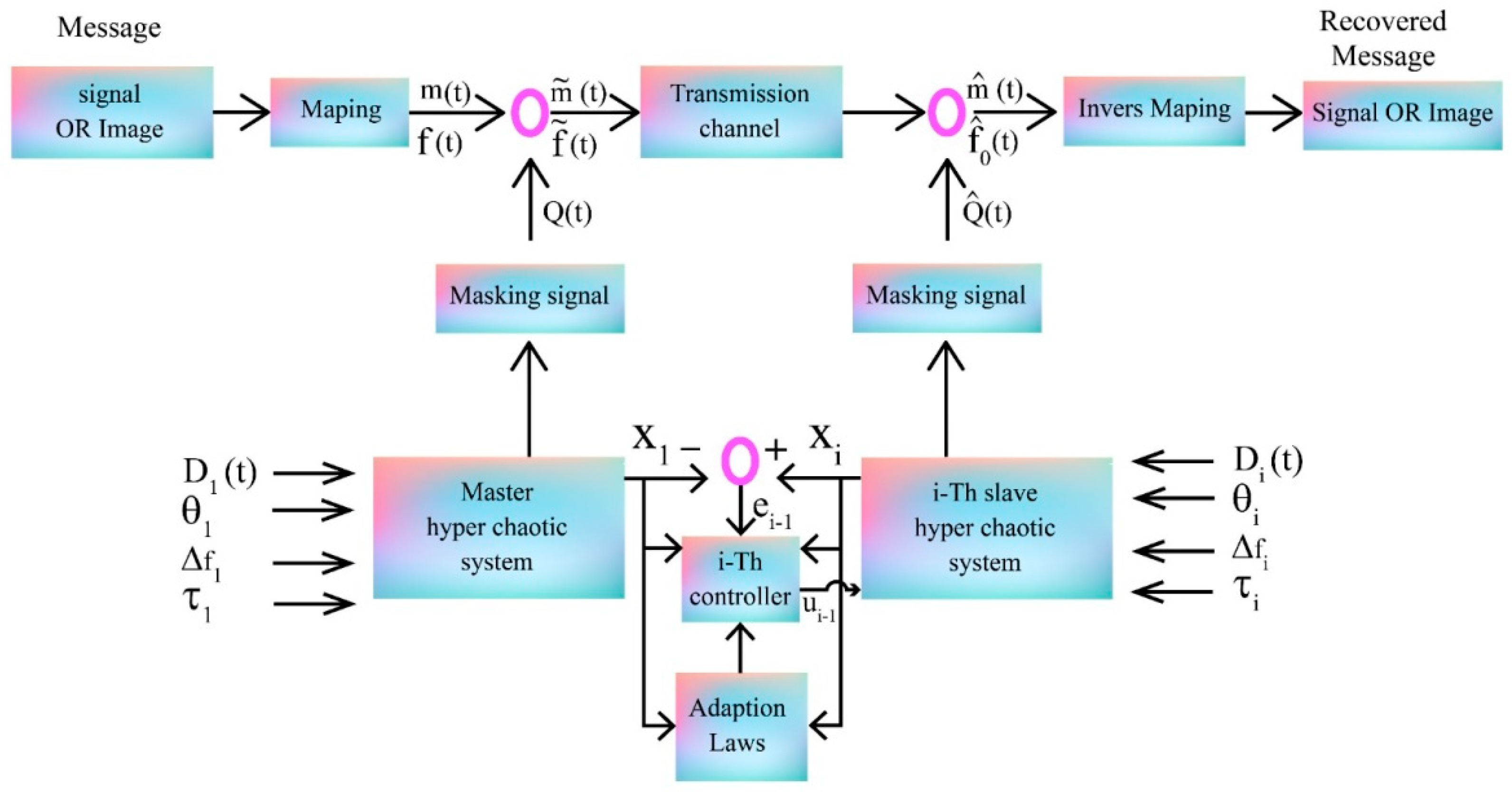
3. Application in Secure Communication Based on Mapping and Chaotic Masking

Chaotic signals have complex behavior and are thus hardly predictable. Using chaotic signals as message carriers in secure communications and cryptography is a suitable and secure solution. Chaotic masking is a way to hide the signal (integration of synchronization with masking) [33,37]. In this approach, the message signal is added to a linear combination of state vector components of the master system. In other words, the message signal information is concealed within the chaotic behavior of the state components, which can enhance communication channel security. The message signal can be recovered from the receiver side by synchronizing the slave system with the master system. Ensuring the synchronization error convergence to zero and the disturbance signals and unknown parameters in the master and slave systems can increase security in the communication channel.
The following lines discuss the application of the proposed method in secure communication for chaotic masking.
Suppose m(t) is a message. It is encrypted with a proper map:
m 0 ( t ) = Λ ( m ( t ) , f ( t ) , a )
where Λ ( m ( t ) , f ( t ) , a ) is a definite and continuous function as the map, and f ( t ) is a definite and continuous signal as a coder. For instance, we can define Λ ( m ( t ) , f ( t ) , a ) as follows:
Λ ( m ( t ) , f ( t ) , a ) = tanh ( a · m ( t ) + f ( t ) )   ,
f ( t ) = 0.2 s i n ( 10 t ) + 0.1 sin ( 20 π t ) + 0.05 c o s ( 2 π t ) , a R
where a is a coefficient so that | a · m ( t ) + f ( t ) | 4 will stand.
Signals m 0 ( t )   , f ( t ) will be masked as follows and transmitted in two components different from the chaotic system:
m ˜ ( t ) = m 0 ( t ) + i = 1 n λ i x i f ˜ ( t ) = f ( t ) + i = 1 n μ i x i
The receiver initially obtains the estimation of signals m 0 ( t ) and f ( t ) . Then, it will calculate m ^ 0 ( t ) , and, ultimately, we will calculate m ^ ( t ) as follows:
m ^ 0 ( t ) = m ˜ ( t ) i = 1 n λ i y i = m 0 ( t ) + i = 1 n λ i x i i = 1 n λ i y i = m 0 ( t ) + i = 1 n λ i e i m 0 ( t )
f ^ ( t ) = f ˜ ( t ) i = 1 n μ i y i = f ( t ) + i = 1 n μ i x i i = 1 n μ i y i = f ( t ) + i = 1 n μ i e i f ( t )
To recover the signal of message m ( t ) , we can do as follows:
m 0 ( t ) = Λ ( m ( t ) , f ( t ) , a ) m ^ 0 ( t ) = Λ ( m ^ ( t ) , f ^ ( t ) , a ) = tanh ( a · m ^ ( t ) + f ^ ( t ) ) m ^ ( t ) = 1 a ( t a n h 1 ( m ^ 0 ( t ) f ^ ( t ) )
Figure 3 shows the chaotic masking in multi-mode synchronization.
Various statistical methods demonstrate the efficiency of synchronization systems of chaotic systems using image encryption. The histogram, correlation, number of pixels change rate (NPCR), unified average changing intensity (UACI), peak signal-to-noise ratio (PSNR), and information entropy parameters were used to demonstrate the efficacy of the proposed synchronization method for the synchronization of fractional-order chaotic systems. The description of the image evaluation parameters is given in references [45,46,47,48,49].

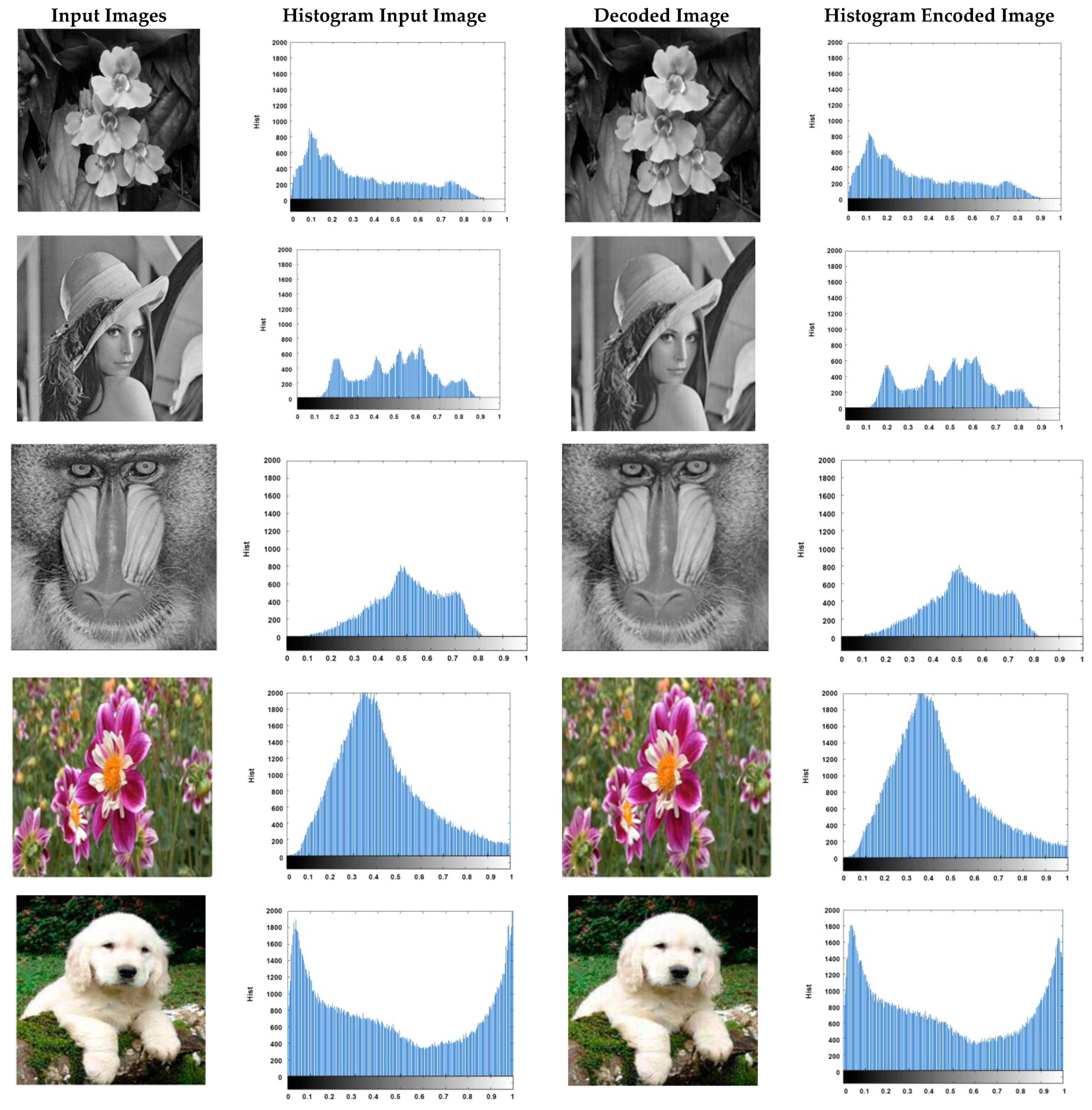
4. Simulation and Results

Here, the fractional-order hyper-chaotic Chen system [47] and two fractional-order Chen systems are considered as master and slave, respectively. They were determined as follows:
{ D q x 11 = θ 11 ( x 12 x 11 ) + x 14 ( t τ 1 ) D q x 12 = θ 21 x 11 x 11 x 13 + θ 13 x 12 D q x 13 = x 11 x 12 θ 14 x 13       D q x 14 = x 12 x 13 + θ 15 x 14
D q x 31 = θ 31 ( x 32 x 31 ) + x 34 t τ 3 + u 21 D q x 32 = θ 31 x 31 x 31 x 33 + θ 33 x 32 + u 22 D q x 33 = x 31 x 32 θ 34 x 33 + u 23 D q x 34 = x 32 x 33 + θ 35 x 34 + u 24 D q x 21 = θ 21 ( x 22 x 21 ) + x 24 t τ 2 + u 11 D q x 22 = θ 22 x 11 x 21 x 23 + θ 23 x 22 + u 12 D q x 23 = x 21 x 22 θ 24 x 13 + u 13 D q x 24 = x 22 x 13 + θ 25 x 14 + u 14
where θ 11 ,   θ 12 ,   θ 13 ,   θ 14 ,   θ 15 are unknown parameters. When θ i 4 = 0.3 ,   θ i 1 = 35 ,   θ i 2 = 3 ,   θ i 3 = 12 ,   θ i 5 = 7 ,   i = 1 , 2 , 3 , then systems (64) and (65) are chaotic systems. The expressions:
u 1 = [ u 11 , u 12 , u 13 , u 14 ] T , u 2 = [ u 21 , u 22 , u 23 , u 24 ] T
are control inputs and
f 1 ( x 1 ) = [ 0 x 11 x 13 x 11 x 12 x 12 x 13 ]   ,   F 1 ( x 1 ) = [ ( x 12 x 11 ) x 11 x 12 x 14 ]
f 3 ( x 3 ) = [ 0 x 31 x 33 x 31 x 32 x 32 x 33 ]   ,   F 3 ( x 3 ) = [ ( x 32 x 31 ) x 31 x 32 x 34 ]   ,   f 2 ( x 2 ) = [ 0 x 21 x 23 x 21 x 22 x 22 x 23 ]   ,   F 2 ( x 2 ) = [ ( x 22 x 31 ) x 21 x 22 x 24 ]
Error dynamics systems are attained as follows:
{ D q e 11 = θ 21 x 22 x 21 θ 11 x 12 x 11 + x 24 t τ 2 x 14 t τ 1 + u 11 D q e 12 = θ 22 x 21 x 21 x 23 + θ 23 x 23 + θ 12 x 11 + x 11 x 13 θ 13 x 31 + u 12 D q e 13 = x 21 x 22 θ 24 x 23 + x 11 x 12 + θ 14 x 13 + u 13 D q e 14 = x 22 x 13 + θ 2 x 24 + x 12 x 13 θ 15 x 14 + u 14
{ D q e 21 = θ 31 x 32 x 31 θ 11 x 12 x 11 + x 34 t τ 2 x 14 t τ 1 + u 21 D q e 21 = θ 32 x 31 x 31 x 33 + θ 33 x 33 + θ 12 x 11 + x 11 x 13 θ 13 x 31 + u 22 D q e 23 = x 31 x 32 θ 34 x 33 + x 11 x 12 + θ 14 x 13 + u 23 D q e 24 = x 32 x 33 + θ 35 x 34 + x 12 x 13 θ 15 x 14 + u 24
In order to simulate, the initial states of the master system and two slave systems are chosen as follows:
x 1 ( 0 ) = [ 10 10 10 10 ] x 2 ( 0 ) = [ 2 2 2 2 ] x 3 ( 0 ) = [ 3 3 3 3 ]
It is assumed that the initial values of the adaptive parameters are as follows:
θ ^ 1 ( 0 ) = [ 3 3 3 3 ] θ ^ 2 ( 0 ) = [ 3 3 3 3 ] θ ^ 3 ( 0 ) = [ 4 4 4 4 ] σ i = 10 .   i = 1 , 2 , 3 , 4 , 5
The parameters of the controller gains K i 1 are as follows:
K 1 = [ 12 0 0 0 0 12 0 0 0 0 12 0 0 0 0 12 ] , K 2 = [ 12 0 0 0 0 12 0 0 0 0 12 0 0 0 0 12 ]
Time-varying delay for master and slave systems has been considered as below:
τ 1 ( t ) = { 1                   0 t 2 3               2 t 4 1                       t 4 τ 2 ( t ) = { 1                   0 t 3 2               3 t 6.5 1                       t 6.5   τ 3 ( t ) = { 1                 0 t 2.5 3               2.5 t 5.5 1                       t 5.5
Later, phase diagrams for chaotic synchronization systems will be depicted. Figure 4 illustrates the chaotic behavior of the fractional-order system. Master and slave systems display chaotic behavior, and their parameters are determined so that the behavior of all the systems will be chaotic.
As can be seen from Figure 4, the phase curves of all three systems are chaotic.
In the simulations, it is supposed that the main parameters vary with time stepwise. The values of disturbances and uncertainties are supposed as follows:
Δ f 1 = [ 0.01 x 11 2 cos ( x 11 ) 0.02 sin ( x 12 ) 0.015 x 13 cos ( x 13 ) 0.025 sin ( x 14 ) ]   .   g 1 ( x 1 ) = | x 1 | 2 + 20 | x 1 |
Δ f 2 = [ 0.15 sin ( x 21 ) 0.025 x 22 cos ( x 22 ) 0.035 sin ( x 23 ) 0.02 x 24 sin ( x 24 ) ] .   g 2 ( x 2 ) = | x 2 |
Δ f 3 = [ 0.025 x 31 sin ( x 31 ) 0.015 x 31 x 32 sin ( x 32 ) 0.035 sin ( x 33 ) 0.02 x 34 sin ( x 34 ) ] .   g 3 ( x 3 ) = | x 3 | 2 + 14 | x 3 |
D 1 = [ 0.025 sin ( π 3 t ) 0.05 sin ( π 3 t ) 0.05 sin ( π 6 t ) 0.04 sin ( π 5 t ) ] D 2 = [ 0.035 sin ( π 3 t ) 0.045 sin ( π 3 t ) 0.025 sin ( π 5 t ) 0.03 sin ( π 6 t ) ] D 3 = [ 0.015 sin ( π 3 t ) 0.025 sin ( π 2 t ) 0.035 sin ( π 10 t ) 0.01 sin ( π 25 t ) ]
The estimation errors of the system parameters and time delay errors are shown in Figure 5. The paths of error dynamics systems and control efforts are exhibited in Figure 6.
Figure 5 shows that the parameters and time delay errors in the multi-mode synchronization properly converge to zero despite the uncertainty and disturbance. The figure shows minimal fluctuation. Therefore, the synchronization approach produced successful results despite the parametric changes. Figure 5 depicts the multi-mode synchronization errors during disturbance and structural uncertainty. Figure 6 presents the error values for the disturbance and uncertainty boundaries estimation.
As indicated in Figure 6,despite the disturbance and uncertainty, the errors were large initially and then approached zero with very little fluctuation. There were fluctuations in these control efforts. Synchronization errors altered slightly with parameter variation, which rapidly converged to zero over time.
Figure 7 indicates that the errors in estimating the uncertain boundaries were initially large due to the initial values of the parameters but are approximated to zero over time. Additionally, the errors related to the uncertainty have converged with very little oscillation to near-zero values. The proper and fast estimation of error boundaries as well as the rapid identification of system parameters leads to proper controller performance. Overall, despite the disturbances, uncertainties, and parametric changes in the master and slave hyper-chaotic systems, the multi-mode synchronization, with the help of the proposed adaptive controller, performed desirably and produced excellent results.

5. Experiment Results

This section describes the results of the synchronization method of the fractional-order Chen chaotic systems for image encryption. First, the images used to perform the experiments were investigated. In the next stage, the encrypted images were represented using the synchronization methods of the fractional-order Chen chaotic systems for q = 0.97, followed by illustrating the histogram of the encrypted images for q = 0.97. Finally, various statistical parameters indicated the effectiveness of the synchronization methods with the fractional-order chaotic system.
Figure 8 illustrates the results obtained from the encryption and decryption results of the proposed secure communication design in five benchmark images.
Figure 8 shows the proper encryption and decryption of the five benchmarks. Figure 8 gives a more precise evaluation by comparing the histograms of the main and recovered images.
Figure 9 shows the main images on the left. In the next column, the histogram of the encrypted image is illustrated. The third column depicts the recovered image. The fourth column shows the histogram of the recovered image. This figure reveals that the histograms of the main image and recovered images have slight differences. However, for more precise analysis, Table 1 demonstrates the results of various statistical criteria. This table shows histogram criteria, correlation, UACI, NPCR, PSNR, and information entropy.
Table 1 reveals that the histograms obtained from the main and the recovered images have slight differences. The correlation between the main and the recovered images is extremely close to 1. The NPCR is approximately 100%. Moreover, good values were obtained for UACI and PSNR. All five images have an information entropy greater than 7. The results suggest that the proposed communication design method successfully encrypted and recovered the main images.

6. Discussion, Advantages and Disadvantages, and Future Works

This paper presents a new secure communication based on Chen fractional order-order chaotic synchronization. This study mainly aims to propose a synchronization method based on multi-mode adaptive control and the Chen fraction order chaos system to encode images. In this work, experiments on five benchmark images were used with 256 × 256 dimensions. Next, the cryptographic method based on synchronization of the Chen fractional order chaos system was applied to benchmark images. The fractional order Chen chaotic system had different delay and q values in this section. Moreover, the presence of an unknown delay factor in the systems complicated the synchronization problem.
Next, the masking technique of chaotic systems was used to encode images. Then, the parameters of histogram, correlation, N.P.C.R., U.A.C.I., P.S.N.R., and information entropy for benchmark images were obtained to demonstrate the efficiency of the proposed synchronization method. The experimental results indicated that the Chen fractional order synchronization method performed successfully. Derivative change varies the behavior of the system as a whole. This is an essential point in cryptography that reduces the possibility of decryption. Considering that the image data are combined with chaotic signals, the amount of security in encryption is sufficiently high. In this mechanism, the parameters of system and time delays are unknown. Moreover, the presence of nonlinear uncertainty makes its detection harder. Results from the rigorous security analysis (fractional order, correlation coefficient, entropy, NPCR, etc.) proved that the proposed method was robust and that the proposed scheme had a high security order. Thus, it can be used for real-time transmission of other images.
Table 2 indicates the high efficiency of the proposed method compared to other studies.
According to Table 2, it can be perceived that our proposed method has a high efficiency compared to other research.
Reviewing the previous studies indicates that little attention has been paid to time delays in communication designs with fractional chaotic system synchronization. The available secure communication synchronization designs ignore unknown time delays, exogenous disturbances, and unknown parameters at the same time. However, our proposed design is comprehensive, considers all factors, and is accompanied by a new function introduced for secure communication based on a flexible map with time-varying coding. The simulations showed that the proposed algorithm performed flawlessly against parameter changes, disturbance, time delays, and uncertainty. The guarantee of system stability is based on Lyapunov’s function. The main reason for the proper performance of the proposed method lies in the form of updated rules obtained in the article; these rules were defined in such a way that the necessary and sufficient conditions for stability in the concept of Mittag-Leffler were established. On the other hand, the method can quickly estimate the parameters and the error of estimating the disturbance and uncertainty boundaries, which results in a faster reaction of the controller against undesirable factors. In general, the proposed method meets all the requirements and has the ability to be implemented in different applications.
In the proposed method, four significant and real factors, including disturbance, uncertainty, time delays, and parameter changes, are considered simultaneously, which helps achieve the highest performance. It is also beneficial in practical implementations. Still, the presented approach applies to a variety of chaotic systems. The resulting control law is considered as an explicit and continuous function. Additionally, the proposed theorems have the ability of two types of multi-mode synchronization. Additionally, the amplitude of the control function is generally significant in the proposed method; if the changes in the parameters are permanent and at a high rate, the recommended algorithm will not yield outstanding performance.
Being based on the Caputo fractional-order derivative can be considered one of the disadvantages of this method. Moreover, parameter changes are only considered as a step change. Proving equivalence between the two types of synchronization, proving convergence of all the errors to zero in the presence of disturbance and uncertainty, the continuation of control laws, and proving efficiency are some of the advantages of this proposed method. To develop the proposed method and solve its weaknesses, we must do as follows: develop the proposed method for other fractional-order derivatives, develop the proposed method for parameters with permanent changes, and analyze the application of the proposed method in secure communication.
It is recommended that future research should address the values of time-varying fractional orders, since reference [56] suggests that this could describe the system more effectively. As future tasks in the synchronization method section, first-and-second-order fuzzy controllers can be adopted. Due to the uncertainty in medical data, fuzzy systems (type 1 and type 2) are highly productive. Modeling chaotic systems using fuzzy systems and fuzzy controller design can provide better answers to the synchronization problem. Applying a fuzzy polynomial system is highly effective in chaotic systems modeling and in their synchronization.

7. Conclusions

This paper investigated the multi-mode synchronization of fractional-order hyper-chaotic systems in the presence of uncertainty, disturbance, time delays, and parameters with stepwise changes in both transmission and circular modes. First, the results confirmed that they are equivalent to the synchronization method. Then, by defining the appropriate Lyapunov function and proofing the theorems, the rules for updating the parameters, as well as error estimating the disturbance and uncertainty boundaries, were assigned. Nonetheless, it should be noted that the stability of the dynamical synchronization system guarantees that all of the synchronization errors, the parameter estimation errors, the disturbance boundary estimation errors, and the uncertainty boundary estimation errors converge to zero. Determining the control law as an explicit and continuous function inhibited chattering. The results also indicated that the rate of change of parameters was not high since the proposed algorithm still displayed an acceptable performance. Simulations were conducted in the presence and absence of disturbance and uncertainty to investigate the effectiveness of the proposed method. The proposed controller reduced synchronization errors, disturbance errors, and uncertainties to zero with low fluctuation near zero, despite changes in time-varying parameters of hyper-chaotic systems. During the parameters changing, a small deviation in synchronization errors was quickly depreciated.
Moreover, unknown time delays were considered. With the help of adaptive regulations, these delays were estimated and used in equations of control effort. Despite these delays, the results revealed that synchronization was appropriately conducted. Additionally, a novel masking design was proposed using the hyperbolic tangent modulation function. To assess this design, benchmark images were encrypted. Various statistical criteria including PSNR, UACI, NPCR, histogram, and correlation were analyzed. The simulation results indicated that the proposed design was successful. The obtained higher efficiency results clearly demonstrated the superiority of the proposed method.

Author Contributions

Conceptualization, A.A.K.J., R.A. and A.Z.; methodology, A.A.K.J., R.A. and A.Z.; software, A.A.K.J. and A.Z.; validation, A.A.K.J., R.A. and A.Z.; formal analysis, A.A.K.J. and S.B.; investigation, A.A.K.J., R.A. and A.Z.; resources, A.A.K.J. and A.Z.; data curation, A.A.K.J. and A.Z.; writing—original draft preparation, A.A.K.J., R.A. and A.Z.; writing—review and editing, A.A.K.J. and A.Z.; visualization, A.A.K.J., R.A., S.B. and A.Z.; supervision, A.Z. All authors have read and agreed to the published version of the manuscript.

Funding

This research received no external funding.

Institutional Review Board Statement

Not applicable.

Informed Consent Statement

Not applicable.

Data Availability Statement

Not applicable.

Conflicts of Interest

The authors declare no conflict of interest.

References

  1. Rosset, C.; Rosset, A.; Ratib, O. General consumer communication tools for improved image management and communication in medicine. J. Digit. Imaging 2005, 18, 270–279. [Google Scholar] [CrossRef] [PubMed] [Green Version]
  2. Ratib, O.; Ligier, Y.; Scherrer, J.R. Digital image management and communication in medicine. Comput. Med. Imaging Graph. 1994, 18, 73–84. [Google Scholar] [CrossRef]
  3. Saadaoui, S.; Tabaa, M.; Monteiro, F.; Chehaitly, M.; Dandache, A. Discrete wavelet packet transform-based industrial digital wireless communication systems. Information 2019, 10, 104. [Google Scholar] [CrossRef] [Green Version]
  4. Safi, S.; Thiessen, T.; Schmailzl, K.J. Acceptance and resistance of new digital technologies in medicine: Qualitative study. JMIR Res. Protoc. 2018, 7, e11072. [Google Scholar] [CrossRef]
  5. Nabutovsky, I.; Nachshon, A.; Klempfner, R.; Shapiro, Y.; Tesler, R. Digital cardiac rehabilitation programs: The future of patient-centered medicine. Telemed. E-Health 2020, 26, 34–41. [Google Scholar] [CrossRef] [Green Version]
  6. Meinel, C.; Sack, H. Digital Communication: Communication, Multimedia, Security; Springer: Berlin/Heidelberg, Germany, 2014. [Google Scholar]
  7. Nie, J.; Hu, X. Mobile banking information security and protection methods. In Proceedings of the 2008 International Conference on Computer Science and Software Engineering, Washington, DC, USA, 12–14 December 2008; IEEE: Piscataway, NJ, USA; Volume 3, pp. 587–590. [Google Scholar]
  8. Nemati, H.R.; Yang, L. (Eds.) Applied Cryptography for Cyber Security and Defense: Information Encryption and Cyphering: Information Encryption and Cyphering; I.G.I. Global: Pennsylvania, PA, USA, 2010. [Google Scholar]
  9. Mahmoud, M.S.B.; Pirovano, A.; Larrieu, N. Aeronautical communication transition from analog to digital data: A network security survey. Comput. Sci. Rev. 2014, 11, 1–29. [Google Scholar] [CrossRef]
  10. Wang, Y.; Shi, Y.; Yi, W.; Nie, C. The methods of digital communication system chaotic encryption using the Duffing oscillator. In Proceedings of the 7th International Conference on Signal Processing, Beijing, China, 31 August–4 September 2004; IEEE: Piscataway, NJ, USA; Volume 3, pp. 1845–1848. [Google Scholar]
  11. Liu, Z.; Saberi, A.; Stoorvogel, A.A.; Nojavanzadeh, D. Global regulated state synchronization for homogeneous networks of non-introspective agents in presence of input saturation: Scale-free nonlinear and linear protocol designs. Automatica 2020, 119, 109041. [Google Scholar] [CrossRef]
  12. Zheng, C.D.; Zhang, L. On synchronization of competitive memristor-based neural networks by nonlinear control. Neurocomputing 2020, 410, 151–160. [Google Scholar] [CrossRef]
  13. Bulut, G.G.; GÜler, H. Fuzzy Based Chaotic Synchronization of Chen Systems. In Proceedings of the 2019 1st Global Power, Energy and Communication Conference (GPECOM), Nevsehir, Turkey, 12–15 June 2019; IEEE: Piscataway, NJ, USA; pp. 30–34. [Google Scholar]
  14. Bhalekar, S.; Daftardar-Gejji, V. Synchronization of different fractional order chaotic systems using active control. Commun. Nonlinear Sci. Numer. Simul. 2010, 15, 3536–3546. [Google Scholar] [CrossRef]
  15. Mahmoud, G.M.; Arafa, A.A.; Mahmoud, E.E. On phase and anti-phase combination synchronization of time delay nonlinear systems. J. Comput. Nonlinear Dyn. 2018, 13. [Google Scholar] [CrossRef]
  16. Yu, J.; Chen, B.; Yu, H.; Gao, J. Adaptive fuzzy tracking control for the chaotic permanent magnet synchronous motor drive system via backstepping. Nonlinear Anal. Real World Appl. 2011, 12, 671–681. [Google Scholar] [CrossRef]
  17. Yadav, V.K.; Srivastava, M.; Das, S. Backstepping Control for Combined Function Projective Synchronization among Fractional Order Chaotic Systems with Uncertainties and External Disturbances. In Nonlinear Dynamical Systems with Self-Excited and Hidden Attractors; Springer: Cham, Switzerland, 2018; pp. 115–132. [Google Scholar]
  18. Yu, J.; Le, J.; Liu, D. Synchronization of chaotic system with adaptive transfer function sliding mode method. Optik 2017, 130, 1053–1072. [Google Scholar] [CrossRef]
  19. Yao, Q. Synchronization of second-order chaotic systems with uncertainties and disturbances using fixed-time adaptive sliding mode control. Chaos Solitons Fractals 2020, 142, 110372. [Google Scholar] [CrossRef]
  20. Luo, R.; Su, H.; Zeng, Y. Synchronization of uncertain fractional-order chaotic systems via a novel adaptive controller. Chin. J. Phys. 2017, 55, 342–349. [Google Scholar] [CrossRef]
  21. Lai, Q.; Wan, Z.; Zhang, H. Design and Analysis of Multi scroll Memristive Hopfield Neural Network with Adjustable Memductance and Application to Image encryption. IEEE Trans. Neural Netw. Learn. Syst. 2022. [Google Scholar] [CrossRef]
  22. Lai, Q.; Norouzi, B.; Liu, F. Dynamic analysis, circuit realization, control design and image encryption application of an extended Lü system with coexisting attractors. Chaos Solitons Fractals 2018, 114, 230–245. [Google Scholar] [CrossRef]
  23. Lai, Q.; Lai, C.; Zhang, H.; Li, C. Hidden coexisting hyper-chaos of new memristive neuron model and its application in image encryption. Chaos Solitons Fractals 2022, 158, 112017. [Google Scholar] [CrossRef]
  24. Mboupda Pone, J.R.; Kingni, S.T.; Kol, G.R.; Pham, V.T. Hopf bifurcation, anti-monotonicity and amplitude controls in the chaotic Toda jerk oscillator: Analysis, circuit realization and combination synchronization in its fractional-order form. Automatika 2019, 60, 149–161. [Google Scholar] [CrossRef]
  25. Bhat, M.A.; Khan, A. Multi-switching combination synchronization of different fractional-order non-linear dynamical systems. Int. J. Model. Simul. 2018, 38, 254–261. [Google Scholar] [CrossRef]
  26. Alam, Z.; Yuan, L.; Yang, Q. Chaos and combination synchronization of a new fractional-order system with two stable node-foci. IEEE/CAA J. Autom. Sin. 2016, 3, 157–164. [Google Scholar]
  27. Yadav, V.K.; Kumar, R.; Leung, A.Y.T.; Das, S. Dual phase and dual anti-phase synchronization of fractional order chaotic systems in real and complex variables with uncertainties. Chin. J. Phys. 2019, 57, 282–308. [Google Scholar] [CrossRef]
  28. Li, B.; Zhou, X.; Wang, Y. Combination synchronization of three different fractional-order delayed chaotic systems. Complexity 2019, 2019, 1–9. [Google Scholar] [CrossRef] [Green Version]
  29. Khan, A.; Bhat, M.A. Multi-switching combination–combination synchronization of non-identical fractional-order chaotic systems. Math. Methods Appl. Sci. 2017, 40, 5654–5667. [Google Scholar] [CrossRef]
  30. Khan, A.; Nigar, U. Sliding mode disturbance observer control based on adaptive hybrid projective compound combination synchronization in fractional-order chaotic systems. J. Control Autom. Electr. Syst. 2020, 31, 885–899. [Google Scholar] [CrossRef]
  31. Kekha Javan, A.A.; Shoeibi, A.; Zare, A.; Hosseini Izadi, N.; Jafari, M.; Alizadehsani, R.; Moridian, P.; Mosavi, A.; Acharya, U.R.; Nahavandi, S. Design of Adaptive-Robust Controller for Multi-State Synchronization of Chaotic Systems with Unknown and Time-Varying Delays and Its Application in Secure Communication. Sensors 2021, 21, 254. [Google Scholar] [CrossRef] [PubMed]
  32. Khan, A.; Jahanzaib, L.S.; Trikha, P. Changing dynamics of the first, second and third approximations of the exponential chaotic system and their application in secure communication using synchronization. Int. J. Appl. Comput. Math. 2021, 7, 1–26. [Google Scholar] [CrossRef]
  33. Mohadeszadeh, M.; Pariz, N. An application of adaptive synchronization of uncertain chaotic system in secure communication systems. Int. J. Model. Simul. 2021, 42, 143–152. [Google Scholar] [CrossRef]
  34. Khan, A.; Trikha, P.; Jahanzaib, L.S. Secure communication: Using synchronization on a novel fractional order chaotic system. In Proceedings of the 2019 International Conference on Power Electronics, Control and Automation (ICPECA), New Delhi, India, 16–17 November 2019; IEEE: Piscataway, NJ, USA; pp. 1–5. [Google Scholar]
  35. Balamash, A.S.; Bettayeb, M.; Djennoune, S.; Al-Saggaf, U.M.; Moinuddin, M. Fixed-time terminal synergetic observer for synchronization of fractional-order chaotic systems. Chaos Interdiscip. J. Nonlinear Sci. 2020, 30, 073124. [Google Scholar] [CrossRef]
  36. Khan, A.; Jahanzaib, L.S.; Khan, T.; Trikha, P. Secure Communication: Using Fractional Matrix Projective Combination Synchronization. Available online: https://aip.scitation.org/doi/10.1063/5.0018974 (accessed on 28 April 2022).
  37. Houmor, T.; Zerimeche, H.; Berkane, A. A secure communication Scheme based on adaptive modified projective combination synchronization of fractional-order hyper-chaotic systems. In Proceedings of the 9th (Online) International Conference on Applied Analysis and Mathematical Modeling (ICAAMM21), Istanbul, Turkey, 11–13 June 2021; p. 73. [Google Scholar]
  38. Babu, N.R.; Kalpana, M.; Balasubramaniam, P. A novel audio encryption approach via finite-time synchronization of fractional order hyperchaotic system. Multimed. Tools Appl. 2021, 80, 18043–18067. [Google Scholar] [CrossRef]
  39. Vaseghi, B.; Mobayen, S.; Hashemi, S.S.; Fekih, A. Fast reaching finite time synchronization approach for chaotic systems with application in medical image encryption. IEEE Access 2021, 9, 25911–25925. [Google Scholar] [CrossRef]
  40. Aguila-Camacho, N.; Duarte-Mermoud, M.A.; Gallegos, J.A. Lyapunov functions for fractional order systems. Commun. Nonlinear Sci. Numer. Simul. 2014, 19, 2951–2957. [Google Scholar] [CrossRef]
  41. Chen, W.; Dai, H.; Song, Y.; Zhang, Z. Convex Lyapunov functions for stability analysis of fractional order systems. IET Control Theory Appl. 2017, 11, 1070–1074. [Google Scholar] [CrossRef]
  42. Matignon, D. Stability results for fractional differential equations with applications to control processing. Comput. Eng. Syst. Appl. 1996, 2, 963–968. [Google Scholar]
  43. Chen, X.; Park, J.H.; Cao, J.; Qiu, J. Sliding mode synchronization of multiple chaotic systems with uncertainties and disturbances. Appl. Math. Comput. 2017, 308, 161–173. [Google Scholar] [CrossRef]
  44. Hegazi, A.S.; Matouk, A.E. Dynamical behaviors and synchronization in the fractional order hyper-chaotic Chen system. Appl. Math. Lett. 2011, 24, 1938–1944. [Google Scholar] [CrossRef] [Green Version]
  45. Kumar, S.; Panna, B.; Jha, R.K. Medical image encryption using fractional discrete cosine transform with chaotic function. Med. Biol. Eng. Comput. 2019, 57, 2517–2533. [Google Scholar] [CrossRef] [PubMed]
  46. Liu, J.; Tang, S.; Lian, J.; Ma, Y.; Zhang, X. A novel fourth order chaotic system and its algorithm for medical image encryption. Multidimens. Syst. Signal. Process. 2019, 30, 1637–1657. [Google Scholar] [CrossRef]
  47. Li, Y.; Chen, Y.; Podlubny, I. Stability of fractional-order nonlinear dynamic systems: Lyapunov direct method and generalized Mittag–Leffler stability. Comput. Math. Appl. 2010, 59, 1810–1821. [Google Scholar] [CrossRef] [Green Version]
  48. Platas-Garza, M.A.; Zambrano-Serrano, E.; Rodríguez-Cruz, J.R.; Posadas-Castillo, C. Implementation of an encrypted-compressed image wireless transmission scheme based on chaotic fractional-order systems. Chin. J. Phys. 2021, 71, 22–37. [Google Scholar] [CrossRef]
  49. Mahmoud, E.E.; Jahanzaib, L.S.; Trikha, P.; Alkinani, M.H. Anti-synchronized quad-compound combination among parallel systems of fractional chaotic system with application. Alex. Eng. J. 2020, 59, 4183–4200. [Google Scholar] [CrossRef]
  50. Peng, Z.; Yu, W.; Wang, J.; Wang, J.; Chen, Y.; He, X.; Jiang, D. Dynamic analysis of seven-dimensional fractional-order chaotic system and its application in encrypted communication. J. Ambient. Intell. Humaniz. Comput. 2020, 11, 5399–5417. [Google Scholar] [CrossRef]
  51. Jahanzaib, L.S.; Trikha, P.; Baleanu, D. Analysis and application using quad compound combination anti-synchronization on novel fractional-order chaotic system. Arab. J. Sci. Eng. 2021, 46, 1729–1742. [Google Scholar] [CrossRef]
  52. Ibraheem, A. Multi-switching dual combination synchronization of time delay dynamical systems for fully unknown parameters via adaptive control. Arab. J. Sci. Eng. 2020, 45, 6911–6922. [Google Scholar] [CrossRef]
  53. Li, Y.; Li, C. Complete synchronization of delayed chaotic neural networks by intermittent control with two switches in a control period. Neurocomputing 2016, 173, 1341–1347. [Google Scholar] [CrossRef]
  54. Kim, J.; Jin, M. Synchronization of chaotic systems using particle swarm optimization and time-delay estimation. Nonlinear Dyn. 2016, 86, 2003–2015. [Google Scholar] [CrossRef]
  55. Guo, J.; Ma, C.; Wang, Z.; Zhang, F. Time-Delay Characteristics of Complex Lü System and Its Application in Speech Communication. Entropy 2020, 22, 1260. [Google Scholar] [CrossRef] [PubMed]
  56. Jahanshahi, H.; Sajjadi, S.S.; Bekiros, S.; Aly, A.A. On the development of variable-order fractional hyper-chaotic economic system with a nonlinear model predictive controller. Chaos Solitons Fractals 2021, 144, 110698. [Google Scholar] [CrossRef]
Figure 1. Transmission multi-mode synchronization.
Bdcc 06 00051 g001
Figure 2. Circular multi-mode synchronizations.
Bdcc 06 00051 g002
Figure 3. Block diagram of chaotic masking with multi-state synchronization.
Bdcc 06 00051 g003
Figure 4. Phase diagrams for master and slave systems. (a) Master System, (b) slave System 1, (c) slave system 2.
Bdcc 06 00051 g004
Figure 5. Estimation of parameters and time delay errors in multi-mode synchronization obtained during disturbance time delay and uncertainty. ((c) indicates time delay errors and (a,b,d) indicate estimation of errors uncertainty).
Bdcc 06 00051 g005
Figure 6. Curves of synchronization errors obtained during disturbance and uncertainty. (subfigures (a,b) show dynamic state errors and subfigures (c,d) show control efforts).
Bdcc 06 00051 g006
Figure 7. Error curves obtained for estimating the uncertain boundaries (right) and disturbances (left).
Bdcc 06 00051 g007
Figure 8. Displayed Benchmark images encryption using synchronization of the fractional-order Chen systems (q = 0.97).
Bdcc 06 00051 g008
Figure 9. Displayed histograms for various Benchmark images encrypted using synchronization of the fractional-order chaotic system (q = 0.97).
Bdcc 06 00051 g009
Table 1. Statistical metrics Benchmark images (q = 0.97).
ImagesHistogramCorrelationDifferential AttackPSNRInformation Entropy
MainEncryptedDecodedNPCR (%)UACI (%)
Image 136,233.04687510,278,639.6328135,454.914060.999699.9933.4643.10497.590
Image 240,953.96093810,271,802.3828140,603.992180.999399.9833.5542.88797.435
Image 361,975.7421010,270,160.9609370,547.039000.998999.6933.1643.05297.210
Image 475,071.2421883,805,961.02343875,522.0078130.999699.6133.4645.79737.421
Image 517,756.5078133,806,198.53125017,534.6718750.999899.9233.4743.90777.822
Table 2. Comparison of the proposed method with other related works.
ReferenceDatasetTypes of DataEncryption MethodDetails Encryption MethodType of DelayDetails of Method
Unknown ParametersDisturbance
[30]sinusoids signal-Fractional-Order Chaotic SystemsGenesio–Tesi system
[31]Voltage signal-Fractional-Order Chaotic SystemsSeven-dimensional fractional-order chaotic system
[32]sinusoids signal-Fractional-Order Chaotic SystemsExponential Chaotic System
[33]sinusoids signal-Fractional-Order Chaotic SystemsFO complex chaotic Lü system
[34]sinusoids signal-Fractional-Order Chaotic SystemsA Novel Fractional Order Chaotic System
[35]square signal-fractional-order chaotic systemsChua system
[36]sinusoids signal-fractional-order chaotic systemsFractional chaotic T system via matrix projective
[37]sinusoids signal-fractional-order chaotic systemsfractional-order Chen and lu hyper-chaotic systems
[39]Benchmark and
Medical Image
Color imagesInteger-order chaotic systemsFast Reaching Finite Time synchronization
[50]Benchmark ImagesColor imagesFractional order systemFractional Order Chaotic Systems
[51]Benchmark ImagesGray Scale ImagesFractional order systemFractional-Order Simplest Chaotic
[52]----Constant-known
[53]----Constant-known
[54]-sine signal-chaotic maskingTime varying-known
[55]“Travelling” music in Matlabspeech signalcomplex Lü systemsself-time-delay synchronization and
chaotic masking
constant-known
Proposed methodBenchmarks ImagesGray Scale & color ImagesFractional order systemMulti-Mode Synchronization of Fractional-Order Chaotic SystemsTime varying-unknown
Publisher’s Note: MDPI stays neutral with regard to jurisdictional claims in published maps and institutional affiliations.

