
Text Classification Based on the Heterogeneous Graph Considering the Relationships between Documents

1
School of Science and Engineering, Ibaraki University, Hitachi 316-8511, Japan
2
Department of Computer and Information Sciences, Faculty of Engineering, Ibaraki University, Hitachi 316-8511, Japan
*
Author to whom correspondence should be addressed.
Big Data Cogn. Comput. 2023, 7(4), 181; https://0-doi-org.brum.beds.ac.uk/10.3390/bdcc7040181
Submission received: 7 November 2023
/
Revised: 11 December 2023
/
Accepted: 11 December 2023
/
Published: 13 December 2023
(This article belongs to the Special Issue Advances in Natural Language Processing and Text Mining)
Abstract
:Text classification is the task of estimating the genre of a document based on information such as word co-occurrence and frequency of occurrence. Text classification has been studied by various approaches. In this study, we focused on text classification using graph structure data. Conventional graph-based methods express relationships between words and relationships between words and documents as weights between nodes. Then, a graph neural network is used for learning. However, there is a problem that conventional methods are not able to represent the relationship between documents on the graph. In this paper, we propose a graph structure that considers the relationships between documents. In the proposed method, the cosine similarity of document vectors is set as weights between document nodes. This completes a graph that considers the relationship between documents. The graph is then input into a graph convolutional neural network for training. Therefore, the aim of this study is to improve the text classification performance of conventional methods by using this graph that considers the relationships between document nodes. In this study, we conducted evaluation experiments using five different corpora of English documents. The results showed that the proposed method outperformed the performance of the conventional method by up to 1.19%, indicating that the use of relationships between documents is effective. In addition, the proposed method was shown to be particularly effective in classifying long documents.
1. Introduction
Text classification is the task of inferring the correct label for a given document from a set of predefined labels. This text classification technique has been used in applications to automate the task of classifying documents by humans. Many researchers are interested in the development of applications that use document classification techniques for spam classification, topic labeling, and sentiment analysis.
Recently, Graph Convolutional Neural networks (GCNs) [1], which can take advantage of data in graph structures, have been used to solve text classification tasks. TextGCN [2], VGCN-BERT [3], and BertGCN [4] are examples of text classification methods that utilize data from graph structures. In TextGCN [2], word and document nodes are represented on the same graph (heterogeneous graph), which is input into the GCN. VGCN-BERT [3] constructs a graph based on the word embedding in Bidirectional Encoder Representations from Transformers (BERT) and word co-occurrence information and learns by inputting the graph into Vocabulary Graph Convolutional Network (VGCN). BertGCN [4] is a text classification method that combines the advantages of transductive learning of GCN with the knowledge obtained from extensive prior learning of BERT. The graphs produced by these graph-based text classification methods use relationships between words and between words and documents. However, conventional graph-based text classification methods do not use relationships between documents. Thus, they are prone to topic drift, in which documents with different contents are associated with each other due to word polysemy. Therefore, we considered that representing the relationship between documents on a graph would improve the performance of text classification.
The purpose of this study is to improve the classification performance of RoBERTaGCN by solving the problems of conventional methods by adding new relationships to the weights of edges between document nodes. First, each document is input into the BERT model to obtain a vector of special tokens [CLS] in its final hidden layer. Next, the cosine similarity of the [CLS] vectors for each document is computed. Then, if it exceeds a predefined threshold, the cosine similarity is added as the weight of the edges between document nodes. This makes the graph an effective graph that considers the relationships among documents. Therefore, we believe that this will improve the accuracy of text classification.
The proposed method is also expected to reduce topic drift, which is a problem in graph-based text classification. Topic drift is a problem in which documents on different topics are associated through words with multiple meanings. For example, the word “apple” can represent either a fruit or an IT company. In this case, topics about fruits and topics about electronic devices such as smartphones could be mixed. In the proposed method, relationships between documents are added directly between document nodes. Since document information can be propagated without going through word nodes, the proposed method is expected to be effective in reducing topic drift.
This paper is organized as follows. In Section 2, we describe traditional methods of text classification and existing research on text classification using neural networks and/or graph neural networks. In Section 3, the structure of graph created in RoBERTaGCN and the processing after graph construction are described. In Section 4, we describe the graph structure of the proposed method. In Section 5, we describe the experiments we conducted to evaluate the proposed method and show the experimental results. In Section 6, we discuss the experimental results presented in Section 5 and conclude in Section 7.
The aim of this paper is to solve the problem of conventional methods and improve the classification performance of conventional methods by adding cosine similarity to the edges between document nodes. In this paper, we make the following contributions.
- We propose the text classification method that solves the problem of conventional methods that do not consider relationships between documents.
- The proposed method is effective for text classification, especially for long documents.
- We identify the optimal values of the parameters that control the balance between the predictions of BERT and GCN.
An early version of the present study was presented at PACLIC2022 [5].
2. Related Works
Text classification is one of the most fundamental tasks in the field of natural language processing. Traditional text classification research based on machine learning can be categorized into two main phases: vector representation of text using feature engineering and classification algorithms using machine learning. In feature engineering, text is represented as a vector by converting it into numerical values to minimize information loss so that the text can be processed by a computer. For feature engineering, commonly used features are BOW (Bag-Of-Words) [6], N-gram [7], TF-IDF (Term Frequency-Inverse Document Frequency) [8], co-occurrence relations between words [9] and so on. Several text classification models have been proposed to predict categories of text data based on these features. Among traditional methods for text classification, general classification models such as Naive Bayes [10], Logistic Regression [11], K-Nearest Neighbor [12], Support Vector Machine [13] and Random Forest [14] have been proposed.
Text classification based on neural networks has been extensively studied in recent years. In early research, deep learning architectures were utilized to learn word embeddings from large text corpora, which were then employed for text classification. The most used distributed word embedding methods are Word2vec [15], Glove [16], FastText [17], Long Short-Term Memory (LSTM) [18], ELMo [19], BERT [20] and RoBERTa [21]. Wang et al. introduced Label-Embedding Attentive Models (LEAM), which jointly embed words and labels in the same space for text classification, leveraging label descriptions to improve performance [22]. Shen et al. proposed Simple Word-Embedding-based Models (SWEMs), which are models that use word embeddings and parameter-free pooling operations to encode text sequences and demonstrated that the effectiveness of deep learning approaches for text classification [23]. Some recent studies have employed neural networks, such as the Multi-Layer Perceptron (MLP) [24], the Convolutional Neural Network (CNN) [25] and LSTM [26], as classification models. The Deep Average Network (DAN), consisting of two fully connected layers and a softmax layer, learns a sentence vector by averaging the word vectors that consist of the input sentence using pre-trained word embeddings [24].
In recent text classification, some studies have employed graph structures in which the relationships between words and between words and documents are expressed in terms of the weight of the edges between each node. A Graph Neural Network (GNN) [27] is a neural network that learns relationships between nodes through edges connecting them. There are several types of GNNs, depending on their form. Employing GNNs for large-scale text processing comes at a significant cost in terms of computational resources. To remove unnecessary complexity and redundant computations in the model, Wu et al. proposed the Simple Graph Convolution model (Simplified GCN) by repeatedly removing the non-linearities and merging weight matrices between consecutive layers into a single linear transformation [28]. Graph Convolutional Neural Networks (GCNs) [1] is a neural network that learns the relationship between a node of interest and its neighbors by means of convolutional computations that use weights assigned to each edge. A Graph Autoencoder (GAE) [29] is an extension of autoencoder, which extracts important features by dimensionality reduction of input data, to handle graph data as well. A Graph Attention Network (GAT) [30] is a neural network that updates and learns node features by multiplying the weights of edges between nodes by Attention, a coefficient representing the importance of neighboring nodes. GNNs have demonstrated high performance in a wide range of machine learning fields. Text generation, question answering, relation extraction, and machine translation are examples. The success of GNNs in such a wide range of tasks has given researchers reason to study text classification methods based on GNNs. In particular, many text classification methods based on GCNs have been proposed. In TextGCN [2], document and word nodes are represented on the same graph (heterogeneous graph). The graph is then input to the GCN for training. In recent years, text classification methods that combine GCN with pre-trained models such as BERT have also been actively studied. VGCN-BERT [3] constructs a graph based on word co-occurrence information and word embeddings of BERT, which is then input into GCN for training. BertGCN [4] constructs a heterogeneous graph based on BERT word co-occurrence information and document embedding, and it is input into GCN for learning. The detailed description of BertGCN is provided in Section 3.
3. Theoretical Background (RoBERTaGCN, RoBERTaGAT)
In this section, RoBERTaGCN and RoBERTaGAT are explained as theoretical background. Equations (1), (7)–(9), (13) and (14) in this section were taken from RoBERTaGCN [4]. Equation (2) was taken from the literature [31]. Equations (4)–(6) were taken from TF-IDF [8]. Equations (10), (11) and (15) were taken from GAT [30].
BertGCN is a text classification method that combines the knowledge of BERT obtained by large-scale pre-training utilizing large unlabeled data with the transductive learning of GCNs, and was proposed by Lin et al. [4]. In BertGCN, each document is input into BERT, the document vector is extracted from its output, and it is input into GCNs as an initial representation of document nodes together with a heterogeneous graph of documents and words for training.
Lin et al. [4] distinguish the names of learning models according to the trained model and the type of GNN used. The correspondence between pre-trained models and model names is shown in Table 1. In this study, RoBERTaGCN and RoBERTaGAT are targeted for improvement.
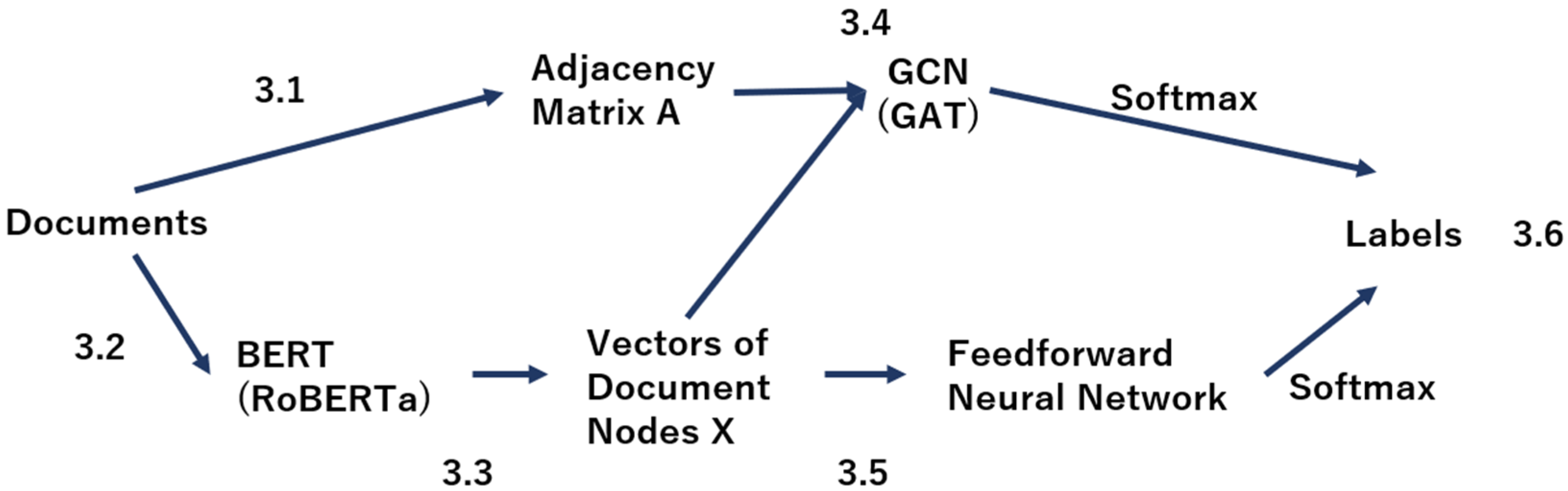
Figure 1 shows an overview of the operation of RoBERTaGCN (RoBERTaGAT). The first step is to construct a heterogeneous graph of words and documents from the documents. Next, the graph information consisting of the weight matrix and the initial node feature matrix is fed into the GCN (GAT), and the document vector is fed into the feedforward neural network. Finally, a linear interpolation of the two predictions is computed and the result is used as the final prediction.
3.1. Constructing Heterogeneous Graph of Words and Documents
The first step is to construct a heterogeneous graph of words and documents from given documents. RoBERTaGCN defines weights between nodes on heterogeneous graphs of words and documents as in (1).
Positive point-wise mutual information (PPMI) is used to weight edges between word nodes. PPMI is a measure of the degree of association between two events and can be viewed as word co-occurrence in natural language processing. PMI is given by Equation (2).
and are words. In RoBERTaGCN, only positive PMI values are used as weights for edges between word nodes. Therefore, as shown in Equation (3), the maximum of the calculated PMI and 0 is added as the weight of edges between word nodes.
Term frequency-inverse document frequency (TF-IDF) is used for the weights of edges between word nodes and document nodes. TF-IDF values are larger for words that occur more frequently in a document but less frequently in other documents, i.e., words that characterize that document. The TF-IDF value can be calculated by multiplying the TF value by the IDF value. The TF value is a value representing the frequency of occurrence of a word. The TF value is calculated by Equation (4).
is a document. is a word that appears in . is the frequency of the word. The IDF value is the reciprocal of the percentage of documents containing a word. The IDF value is computed by Equation (5).
is the total number of documents. is the number of documents in which appears. TF-IDF value is calculated by Equation (6).
As shown in Equation (1), RoBERTaGCN is not able to express the relationship between document nodes in terms of the weights of edges between nodes. This is a point that needs to be improved in this study.
3.2. Tokenizing Documents
Next, each document is converted into a sequence of tokens that can be entered into BERT. A special classification token ([CLS]) is added to the beginning of the document and a special separator token ([SEP]) is added to the end of the document. A document is considered and processed as a single sentence, and each document is normalized to 512 tokens.
3.3. Creating the Initial Node Feature Matrix
Next, initialize the node feature matrix for the GCNs. To obtain this matrix, BERT is used to generate a document embedding, which is then used as the input features of the document node. The initialize the node feature matrix are represented by a matrix , where is the number of documents and is the number of embedding dimensions. Overall, the initial node feature matrix is given by Equation (7), where is the total number of word nodes in the training and test data sets.
3.4. Input into GCN (GAT) and Learning by GCN (GAT)
Heterogeneous graph and initial node feature matrix are given to GCN for training. The output feature matrix of layer is computed by (8).
is the activation function and is the normalized adjacency matrix of . is the weight matrix at layer . is the matrix , which is the input feature matrix of the model. The dimension of the final layer of is (number of embedded dimensions) × (number of output classes). The GCNs’ outputs are treated as final document representations, which are then fed to the softmax layer for classification. This GCNs’ prediction is given by the following Equation (9)
where the function represents the GCNs model. The cross-entropy loss of the labeled document nodes is used to jointly train BERT and GCNs.
When GAT is used, the feature update of node is given by Equation (10).
is a vector, of each node. is some neighborhood of node . is an attention between and . Attention is given by Equation (11).
The attention mechanism is a single-layer feedforward neural network and applying the nonlinearity. GAT’s prediction is given by the following Equation (12).
3.5. Input into Feedforward Neural Network and Learning by Feedforward Neural Network
To speed up convergence and improve performance, RoBERTaGCN optimizes the model with auxiliary classifier that directly operates on the BERT embedding [4]. Specifically, a document embedded representation is input into a Feedforward Neural Network. The output is then fed directly into a softmax function with a weight matrix to create an auxiliary classifier with BERT. The auxiliary classifier predicts the output predictions of the input documents using the following Equation (13).
3.6. Interpolation of Predictions with BERT and GCN (GAT)
To output the result of the linear interpolation as a final prediction, A linear interpolation is computed with the output predictions using RoBERTaGCN and the output predictions using BERT. The result of the linear interpolation is represented by the following Equation (14)
where determines how much weight is given to each prediction. means using the full RoBERTaGCN model, while means using only the BERT model. Given the parameter , the predictions from both models can be balanced. Experiments by Lin et al. using the graph structure in (1) show that is the optimal value of [4].
Similarly for the case using GAT, the final prediction is the result of linear interpolation of the BERT prediction and the GAT prediction. Thus, the final prediction when GAT is used is given by Equation (15).
4. Proposed Method
This section describes the proposed new graph structure. Equation (17) in this section was taken from the literature [31].
The weights of the edges connecting nodes i and j are given by Equation (16).
As shown in Equation (1), RoBERTaGCN represents only the relationships between words and between words and documents as the weight of edges in a graph, but it does not directly consider the relationships between documents. Figure 2 is an image of the graph. In our proposed method, we modified RoBERTaGCN to consider not only these relationships but also the relationship between documents by expressing the weights of edges between document nodes. The weights of the edges between document nodes in Equation (16) represent the cosine similarity between the two nodes i and j, which is a measure of how similar the two documents are. Specifically, the weights of the edges between document nodes are added to the heterogeneous graph by the following three steps.
- Document tokenization: Each document is converted into a sequence of tokens that can be understood by the BERT model. A special classification token ([CLS]) is added to the beginning of the document, and a special separator token ([SEP]) is added to the end of the document. These two tokens are special tokens. [CLS] denotes the beginning of the sentence, and [SEP] denotes the end of the sentence. In this study, a single document was regarded as a single sentence and processed. For long documents (more than 512 words), we extract the first 510 words and add special tokens to make it 512 words long. For short documents (fewer than 510 words), we pad them with 0 s to reach the 512-word limit for BERT.
- Extracting [CLS] embeddings: We feed each tokenized document into BERT to get a [CLS] vector in the last hidden layer. The [CLS] vector is a representation of the entire document, capturing its context.
- Calculating cosine similarity as weights of edges: We calculate the cosine distance between the [CLS] encodings of each document and add edges between corresponding document nodes if the cosine similarity is greater than a predefined threshold, where the weight of each edge is the cosine similarity of the [CLS] vectors.
PPMI is used for the weights of edges between word nodes, and TF-IDF values are used for the weights of edges between word and document nodes. The formulas for calculating PPMI are the same as in Equations (2) and (3). The formulas for calculating TF-IDF are the same as in Equations (4)–(6). Cosine similarity is given by Equation (17). and are the vectors of documents and . is the number of vector dimensions.
The process after graph construction is the same as in Section 3.2, Section 3.3, Section 3.4, Section 3.5 and Section 3.6.
5. Experiments
5.1. Data Set
Experiments were conducted on the five data sets listed in Table 2 to evaluate the performance of the proposed method. Many of the previous studies, including RoBERTaGCN [4] and TextGCN [2], have conducted experiments using these five datasets. Therefore, these five datasets were also used in this study. These data used were the same as those used in RoBERTaGCN. Each dataset was used as is because it had already been split into training and test data. All five datasets were used in the experiments after the preprocessing described in Section 5.3.
- 20-Newsgroups (20NG)
Each document in 20NG is classified into one of the 20 news labels. The number of documents is 18,846 in total. A total of 11,314 documents, corresponding to about 60% of all documents, are training data. 7532 documents, corresponding to about 40% of all documents, are test data.
- R8, R52
Both R8 and R52 are subsets of the dataset (21,578 documents) provided by Reuters. Each document in R8 is classified into one of the eight labels. The number of documents in R8 is 7674 in total. A total of 5485 documents, corresponding to about 71.5% of all documents, are training data. 2189 documents, corresponding to about 28.5% of all documents, are test data. Each document in R52 is classified into one of the 52 labels. The number of documents in R52 is 9100 in total. 6532 documents, corresponding to about 71.8% of all documents, are training data. 2568 documents, corresponding to about 28.2% of all documents, are test data.
- Ohsumed
Ohsumed is a dataset of medical documents from the U.S. National Library of Medicine. The total number of documents is 13,929; each document has one or more associated disease labels from a list of 23 disease labels. In our experiments, we used documents with only one disease label. The total number of documents used was 7400. A total of 3357 documents, corresponding to about 45.4% of all documents, are training data. 4043 documents, corresponding to about 54.6% of all documents, are test data.
- Movie Review (MR)
MR is a dataset used for sentiment classification, and each review is classified into two categories: positive and negative. The number of documents is 10,662 in total. A total of 7108 documents, corresponding to about 66.7% of all documents, are training data. A total of 3554 documents, corresponding to about 33.3% of all documents, are test data.
5.2. Experimental Settings
In this study, three experiments were conducted to evaluate the performance of the proposed method.
Experiment 1.
Experiment to confirm the effectiveness of the proposed method.
In Experiment 1, the experiment is conducted with a threshold of 0.5 and 0.005 increments from 0.95 to 0.995 for the cosine similarity. The classification performance of the proposed method is evaluated by comparing it with the classification performance of the original RoBERTaGCN and other text classification methods. The value of λ was fixed at 0.7. Preliminary experiments were conducted on the validation data to analyze the optimal value for each dataset of the cosine similarity threshold. The optimal values are shown in Table 3.
Experiment 2.
Experiment to analyze the optimal value of λ in the proposed method.
In Experiment 2, we conducted the experiment by changing the value of λ from 0.1 to 0.9 in order to analyze the optimal value of λ for the proposed method using the graph structure in Equation (16). For the threshold value of cosine similarity, we used the threshold value that resulted in the highest classification performance in Experiment 1. In the previous study, only the optimal value for the 20NG data set was shown. Therefore, in this study, the optimal value of λ in five datasets (20NG, R52, R8, Ohsumed, and MR) is clarified through experiments. Then, by analyzing the trend and the characteristics of each dataset, we discuss the relationship between the characteristics of the data and the optimal value of λ.
Experiment 3.
Experiment to confirm classification performance when using GAT.
We verify whether the heterogeneous graphs constructed by the proposed method are effective for other GNN. Specifically, we check the classification performance when GAT is used, and evaluate the effectiveness of the graph structure of the proposed method. In Experiment 3, we set the threshold of cosine similarity and the value of λ that gave the best classification performance based on the results of Experiments 1 and 2.
5.3. Preprocessing
The following three preprocessing steps were applied to all data. These preprocessing steps are the same as those done in RoBERTaGCN [4].
- Step1
- : Noise Removal.
All characters and symbols except alphanumeric characters and certain symbols (( ) , ! ? ‘ ’) were removed as noise.
- Step2
- : Word Normalization.
All alphanumeric characters were normalized to half-width alphanumeric characters. Then, normalized alphanumeric characters are unified into lowercase letters.
- Step3
- : Stop Words Removal.
Stop words in text were removed using stop words list of Natural Language Toolkit (NLTK).
5.4. Experimental Environment
We conducted our experiments using Google Colaboratory Pro+ (5 May 2023). Colaboratory Pro+ is an execution environment for Python 3.6.9 and other languages provided by Google (Mountain View, CA, USA). Table 4 shows the specifications of Google Colaboratory Pro+.
5.5. Evaluation Index
The accuracy was used as the evaluation index for the experiment. In previous studies, including RoBERTaGCN [4] and TextGCN [2], accuracy has been used as an evaluation index, and to make comparing results easier, it was also used in this study. The accuracy is calculated by Equation (18). Positive is the label of the correct answer, and negative is the label of the incorrect answer. Negatives are all the remaining labels except the correct answer label. TP (True-Positive) is the number of items that should be classified as positive that were correctly classified as positive. TN (True-Negative) represents the number of items that should be classified as negative that were correctly classified as negative. FP (False-Positive) indicates the number of cases where items that should have been classified as negative were incorrectly classified as positive. FN (False-Negative) indicates the number of cases where items that should have been classified as positive were incorrectly classified as negative.
5.6. Result of Experiment 1
Table 5 shows the classification performance of the proposed method for each cosine similarity threshold. “×” indicates that the experiment could not be completed due to lack of memory. Furthermore, “-” indicates that the experiment is not described in the reference. Experiments with the same number of edges in are listed together in Table 5.
For all datasets, the proposed method outperforms the original RoBERTaGCN in classification performance at certain thresholds. However, in the experiments using R8, R52, and MR, the proposed method outperformed the original RoBERTaGCN for only one to two threshold values. In other words, those three datasets did not show a stable improvement in classification performance. On the other hand, 20NG outperformed the original RoBERTaGCN in every threshold value from 0.95 to 0.995. Ohsumed also outperformed the original RoBERTaGCN in most threshold values. For 20NG, the proposed method outperformed the original RoBERTaGCN by 0.67% at the threshold of 0.975. The proposed method also outperformed the original RoBERTaGCN by 1.19% at a threshold of 0.965 for Ohsumed.
Compared to the classification performance of methods other than the original RoBERTaGCN, the classification performance of the proposed method was the best for three datasets: 20NG, R8, and Ohsumed. On the other hand, R52 showed the best classification performance of BERT, and MR showed the best performance of RoBERTa. For R52 and MR, Experiment 2 shows that the classification performance of the proposed method is best when the value of λ is set smaller than 0.7. The details are explained in Section 5.7.
5.7. Result of Experiment 2
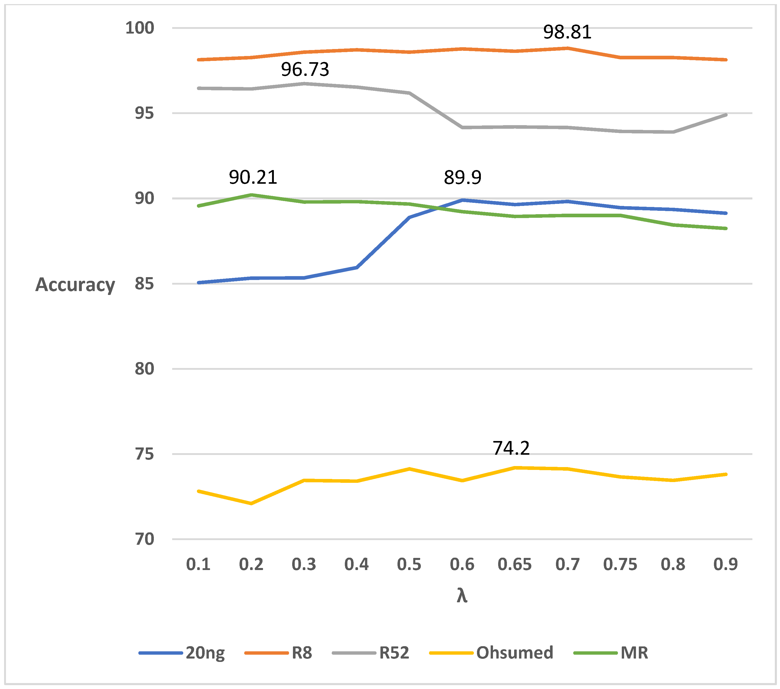
The classification performance of the proposed method for different values of the parameter λ is shown in Figure 3. For 20NG and Ohsumed, the higher the value of λ, the higher the accuracy. For R8, the classification accuracy tends to be higher when the value of λ is set to an intermediate value. For R52 and MR, accuracy is higher when λ is set to a lower value. For R52, when λ is set to 0.3, the classification performance is 96.73%, which is 0.33% higher than the classification performance of BERT in Table 5. For MR, when λ is set to 0.2, the classification performance is 90.21%, which is 0.81% higher than the performance of RoBERTa in Table 5.
5.8. Result of Experiment 3
The classification performance when using GAT is shown in Table 6. When using GAT, the classification performance of the proposed graph outperformed that of original RoBERTaGAT for the three datasets R8, R52, and MR. For R52, the classification performance exceeded that of the original RoBERTaGAT by 0.98%. For MR, the classification performance exceeded that of the original RoBERTaGAT by 0.54%.
6. Discussion
6.1. Effectiveness of the Proposed Method
As shown in Table 5, the classification performance of the proposed method outperforms that of the original RoBERTaGCN on all datasets in the experiments. This indicates that the heterogeneous graphs constructed in the proposed method were effective. Figure 4 shows the percentage of cosine similarity weights added to edges between document nodes with the same label. In all datasets, the percentage of correct answers for cosine similarity is high, indicating that many weights are added to the edges between document nodes with the same label. Therefore, it can be considered that the high classification performance of the proposed method on heterogeneous graphs is due to the fact that more weight is added to the edges between document nodes with the same label.
The results of Experiment 1 in Table 5 show that the classification performance of the proposed method with GCN is particularly high on two datasets, 20NG and Ohsumed. From Table 3, it can be seen that 20NG and Ohsumed are the datasets with the first and second highest average number of words among the datasets used. Therefore, the proposed method using GCN is particularly effective in classifying relatively long documents such as 20NG and Ohsumed.
The results of Experiment 3 in Table 6 show that the classification performance of the proposed method with GAT is particularly high on the two datasets of R52 and MR. Therefore, we can say that the proposed method with GAT is particularly effective in classifying relatively short documents, such as R52 and MR, contrary to the case with GCN.
6.2. Optimal Value of λ for Each Dataset
The results of Experiment 2, shown in Figure 3, indicate that the optimal value of λ is between 0.6 and 0.7 for the three datasets of 20NG, R8, and Ohsumed. Thus, for these three datasets, the classification performance of the proposed method tends to be higher when the value of λ is set higher and the prediction from GCN is more important than BERT. On the contrary, the optimal value of λ in R52 and MR is 0.2~0.3. Therefore, for these two datasets, the classification performance of the proposed method tends to be higher when the value of λ is set lower and the prediction of BERT is more important than GCN. The reason for these two trends is the number of labels. While the number of labels for 20NG, R8, and Ohsumed is 20, 8, and 23, the number of labels for R52 is extremely high (52) and the number of labels for MR is extremely low (2). Therefore, when classifying documents with an extremely high or low number of labels, we found that setting a lower value of λ and focusing on the prediction of BERT yielded higher classification performance. In contrast, when classifying documents with an average number of labels, we found that setting a higher value of λ and focusing on the predictions of GCN yielded higher classification performance.
6.3. Items with Significantly Low Classification Accuracy
Table 7 shows the Average of Cosine Similarity and the Number of Added Edges when the threshold for adding weights to the cosine similarity was set to 0.5. The items marked “×” are those that could not finish adding weights because they ran out of memory during the process of calculating the cosine similarity. When the threshold was set to 0.5, experiments using 20NG, R52, and MR could not be completed due to insufficient memory. Experiments using R8 and Ohsumed could be completed, but the classification performance was significantly lower than the original RoBERTaGCN. This may be due to too many weights being added between document nodes. The number of edges of cosine similarity is more than twice the number of the other two edges in all datasets. The average value of the cosine similarity is between 0.8 and 0.85 in all datasets. Therefore, it is likely that many weights are added between document nodes that do not have the same label and that these weights are noise.
7. Conclusions
In this paper, we propose a text classification method using a graph constructed by adding the cosine similarity of CLS vectors of documents as weights of edges between document nodes in order to solve the problem of conventional text classification methods that do not use relationships among documents. Experiments confirmed that our proposed method, which classifies documents using an effective graph that considers the relationships among documents, outperforms the original RoBERTaGCN and achieves high classification performance. In particular, experiments showed that the proposed method is effective for long documents. The optimal value of λ, a parameter that controls the balance between the prediction results of BERT and GCN, was also clarified. It should be set low when the number of labels in the document to be classified is extremely large or small. On the other hand, experiments showed that when the number of labels in a document is average, setting it high is optimal.
Future work includes using other features instead of cosine similarity and devising a way to handle documents exceeding 510 words.
Author Contributions
Conceptualization, H.N. and M.S.; methodology, H.N.; software, H.N.; validation, H.N.; formal analysis, H.N.; investigation, H.N. and M.S.; resources, H.N.; data curation, H.N.; writing—original draft preparation, H.N.; writing—review and editing, H.N. and M.S.; visualization, H.N.; supervision, H.N. and M.S.; project administration, H.N. and M.S. All authors have read and agreed to the published version of the manuscript.
Funding
This research received no external funding.
Institutional Review Board Statement
Not applicable.
Informed Consent Statement
Not applicable.
Data Availability Statement
The data used in this study is available on GitHub. The data can be accessed online at: https://github.com/ZeroRin/BertGCN/tree/main/data (accessed on 25 October 2023).
Conflicts of Interest
The authors declare no conflict of interest.
References
- Kipf, T.N.; Welling, M. Semi-supervised classification with graph convolutional networks. arXiv 2017, arXiv:1609.02907. [Google Scholar]
- Yao, L.; Mao, C.; Luo, Y. Graph convolutional networks for text classification. In Proceedings of the AAAI Conference on Artificial Intelligence, Honolulu, HI, USA, 27 January–1 February 2019; Volume 33, pp. 7370–7377. [Google Scholar] [CrossRef]
- Lu, Z.; Du, P.; Nie, J.Y. Vgcn-bert: Augmenting bert with graph embedding for text classification. In Proceedings of the European Conference on Information Retrieval, Lisbon, Portugal, 14–17 April 2020; pp. 369–382. [Google Scholar] [CrossRef]
- Lin, Y.; Meng, Y.; Sun, X.; Han, Q.; Kuang, K.; Li, J.; Wu, F. BertGCN: Transductive Text Classification by Combining GCN and BERT. In Findings of the Association for Computational Linguistics: ACL-IJCNLP 2021; Association for Computational Linguistics: Kerrville, TX, USA, 2021; pp. 1456–1462. [Google Scholar] [CrossRef]
- Nakajima, H.; Sasaki, M. Text Classification Using a Graph Based on Relationships Between Documents. In Proceedings of the 36th Pacific Asia Conference on Language, Information and Computation, Manila, Philippines, 20–22 October 2022; pp. 119–125. Available online: https://aclanthology.org/2022.paclic-1.14.pdf (accessed on 16 October 2023).
- Zhang, Y.; Jin, R.; Zhou, Z. Understanding bag-of-words model: A statistical framework. Int. J. Mach. Learn. Cybern. 2010, 1, 43–52. [Google Scholar] [CrossRef]
- Cavnar, W.B.; Trenkle, J.M. N-gram-based text categorization. In Proceedings of SDAIR-94, 3rd Annual Symposium on Document Analysis and Information Retrieval, Las Vegas, NV, USA, 1 September 1994; Citeseer: Las Vegas, NV, USA, 1994; Volume 161175. [Google Scholar]
- Baeza-Yates, R.; Ribeiro-Neto, B. Modern Information Retrieval; ACM Press: New York, NY, USA, 1999; Volume 463. [Google Scholar]
- Figueiredo, F.; Rocha, L.; Couto, T.; Salles, T.; Gonçalves, M.A.; Meira, W., Jr. Word co-occurrence features for text classification. Inf. Syst. 2011, 36, 843–858. [Google Scholar] [CrossRef]
- Maron, E. Automatic indexing: An experimental inquiry. J. ACM 1961, 8, 404–417. [Google Scholar] [CrossRef]
- Ng, A.Y.; Jordan, M.I. On discriminative vs. generative classifiers: A comparison of logistic regression and naive Bayes. In Proceedings of the 14th International Conference on Neural Information Processing Systems: Natural and Synthetic, Vancouver, BC, Canada, 3–8 December 2001; pp. 841–848. [Google Scholar]
- Cover, T.; Hart, P. Nearest neighbor pattern classification. IEEE Trans. Inf. Theory 1967, 13, 21–27. [Google Scholar] [CrossRef]
- Joachims, T. Text categorization with support vector machines: Learning with many relevant features. In Proceedings of the 10th European Conference on Machine Learning, Chemnitz, Germany, 21–23 April 1998; pp. 137–142. Available online: https://0-link-springer-com.brum.beds.ac.uk/chapter/10.1007/BFb0026683 (accessed on 16 October 2023).
- Breiman, L. Bagging predictors. Mach. Learn. 1996, 24, 123–140. [Google Scholar] [CrossRef]
- Mikolov, T.; Chen, K.; Corrado, G.; Dean, J. Efficient estimation of word representations in vector space. arXiv 2013, arXiv:1301.3781. [Google Scholar]
- Pennington, J.; Socher, R.; Manning, C.D. GloVe: Global vectors for word representation. In Proceedings of the 2014 Conference on Empirical Methods in Natural Language Processing (EMNLP), Doha, Qatar, 25–29 October 2014; pp. 1532–1543. [Google Scholar] [CrossRef]
- Joulin, A.; Grave, E.; Bojanowski, P.; Mikolov, T. Bag of Tricks for Efficient Text Classification. arXiv 2016, arXiv:1607.01759. [Google Scholar]
- Hochreiter, S.; Schmidhuber, J. Long short-term memory. Neural Comput. 1997, 9, 1735–1780. [Google Scholar] [CrossRef] [PubMed]
- Peters, M.E.; Neumann, M.; Iyyer, M.; Gardner, M.; Clark, C.; Lee, K.; Zettlemoyer, L. Deep Contextualized Word Representations. In Proceedings of the 2018 Conference of the North American Chapter of the Association for Computational Linguistics: Human Language Technologies, New Orleans, LA, USA, 1–6 June 2018; pp. 2227–2237. Available online: http://aclweb.org/anthology/N18-1202 (accessed on 16 October 2023).
- Devlin, J.; Chang, M.; Lee, K.; Toutanova, K. BERT: Pre-training of Deep Bidirectional Transformers for Language Understanding. In Proceedings of the 2019 Conference of the North American Chapter of the Association for Computational Linguistics: Human Language Technologies, Minneapolis, MN, USA, 2–7 June 2019; pp. 4171–4186. [Google Scholar] [CrossRef]
- Liu, Y.; Ott, M.; Goyal, N.; Du, J.; Joshi, M.; Chen, D.; Levy, O.; Lewis, M.; Zettlemoyer, L.; Stoyanov, V. RoBERTa: A Robustly Optimized BERT Pretraining Approach. arXiv 2019, arXiv:1907.11692. [Google Scholar]
- Wang, G.; Li, C.; Wang, W.; Zhang, Y.; Shen, D.; Zhang, X.; Henao, R.; Carin, L. Joint Embedding of Words and Labels for Text Classification. In Proceedings of the 56th Annual Meeting of the Association for Computational Linguistics, Melbourne, Australia, 15–20 July 2018; pp. 2321–2331. Available online: https://aclanthology.org/P18-1216 (accessed on 16 October 2023).
- Shen, D.; Wang, G.; Wang, W.; Min, M.R.; Su, Q.; Zhang, Y.; Li, C.; Henao, R.; Carin, L. Baseline Needs More Love: On Simple Word-Embedding-Based Models and Associated Pooling Mechanisms. In Proceedings of the 56th Annual Meeting of the Association for Computational Linguistics, Melbourne, Australia, 15–20 July 2018; pp. 440–450. Available online: http://aclweb.org/anthology/P18-1041 (accessed on 16 October 2023).
- Iyyer, M.; Manjunatha, V.; Boyd-Graber, J.; Daumé, H., III. Deep Unordered Composition Rivals Syntactic Methods for Text Classification. In Proceedings of the 53rd Annual Meeting of the Association for Computational Linguistics and the 7th International Joint Conference on Natural Language Processing, Beijing, China, 27–31 July 2015; pp. 1681–1691. [Google Scholar] [CrossRef]
- Kalchbrenner, N.; Grefenstette, E.; Blunsom, P. A Convolutional Neural Network for Modelling Sentences. In Proceedings of the 52nd Annual Meeting of the Association for Computational Linguistics, Baltimore, MD, USA, 22–27 June 2014; pp. 655–665. [Google Scholar] [CrossRef]
- Tai, K.S.; Socher, R.; Manning, C.D. Improved Semantic Representations from Tree-Structured Long Short-Term Memory Networks. In Proceedings of the 53rd Annual Meeting of the Association for Computational Linguistics and the 7th International Joint Conference on Natural Language Processing, Beijing, China, 27–31 July 2015; pp. 1556–1566. [Google Scholar] [CrossRef]
- Scarselli, F.; Gori, M.; Tsoi, A.C.; Hagenbuchner, M.; Monfardini, G. The graph neural network model. IEEE Trans. Neural Netw. 2008, 20, 61–80. [Google Scholar] [CrossRef] [PubMed]
- Wu, F.; Zhang, T.; Souza, A.H.; Fifty, C., Jr.; Yu, T.; Weinberger, K.Q. Simplifying Graph Convolutional Networks. In Proceedings of the 36th International Conference on Machine Learning, Long Beach, CA, USA, 10–15 June 2019; pp. 6861–6871. Available online: https://arxiv.org/abs/1902.07153 (accessed on 16 October 2023).
- Kipf, T.N.; Welling, M. Variational graph auto-encoders. arXiv 2016, arXiv:1611.07308. [Google Scholar]
- Velickovic, P.; Cucurull, G.; Casanova, A.; Romero, A.; Lio, P.; Bengio, Y. Graph attention networks. arXiv 2017, arXiv:1710.10903. [Google Scholar]
- Witten, I.H.; Moffat, A.; Bell, T.C. Managing Gigabytes: Compressing and Indexing Documents and Images; Morgan Kaufmann: San Francisco, CA, USA, 1999. [Google Scholar] [CrossRef]
Figure 1.
Schematic Diagram of the RoBERTaGCN (RoBERTaGAT).

Figure 2.
An image of the proposed graph.

Figure 3.
Classification Performance of the Proposed Method When Changing the Value of λ.

Figure 4.
Accuracy of Cosine Similarity.


Table 1.
Names of the Model.
| Name of Model | Pre-Trained Model | GNN |
|---|---|---|
| BertGCN | bert-base | GCN |
| BertGAT | bert-base | GAT |
| RoBERTaGCN | roberta-base | GCN |
| RoBERTaGAT | roberta-base | GAT |
Table 2.
Information of Data Set.
| Data Set | Average of Words | Number of Documents | Training Data | Test Data |
|---|---|---|---|---|
| 20NG | 206.4 | 18,846 | 11,314 | 7532 |
| R8 | 65.7 | 7674 | 5485 | 2189 |
| R52 | 69.8 | 9100 | 6532 | 2568 |
| Ohsumed | 129.1 | 7400 | 3357 | 4043 |
| MR | 20.3 | 10,662 | 7108 | 3554 |
Table 3.
Optimal Value for Cosine Similarity Threshold.
| Data Set | Optimal Threshold Value |
|---|---|
| 20NG | 0.99 |
| R8 | 0.975 |
| R52 | 0.96 |
| Ohsumed | 0.965 |
| MR | 0.97 |
Table 4.
Google Colaboratory Pro+ Specification Details.
| Memory | GPU | Disk |
|---|---|---|
| 12.69 GB (standard) /51.01 GB (CPU/GPU (high memory)) /35.25 GB (TPU (high memory)) | Tesla V100 (SXM2) /A100 (SXM2) | 225.89 GB (CPU/TPU) /166.83 GB (GPU) |
Table 5.
Classification Performance of the Proposed Method. Experimental results for the baseline methods were provided by [2].
Table 5.
Classification Performance of the Proposed Method. Experimental results for the baseline methods were provided by [2].
| 20NG | R8 | R52 | Ohsumed | MR | |
|---|---|---|---|---|---|
| Text GCN [2] | 86.34 | 97.07 | 93.56 | 68.36 | 76.74 |
| Simplified GCN [28] | 88.50 | - | - | 68.50 | - |
| LEAM [22] | 81.91 | 93.31 | 91.84 | 58.58 | 76.95 |
| SWEM [23] | 85.16 | 95.32 | 92.94 | 63.12 | 76.65 |
| TF-IDF+LR | 83.19 | 93.74 | 86.95 | 54.66 | 74.59 |
| LSTM [21] | 65.71 | 93.68 | 85.54 | 41.13 | 75.06 |
| FastText [12] | 79.38 | 96.13 | 92.81 | 57.70 | 75.14 |
| BERT [15] | 85.30 | 97.80 | 96.40 | 70.50 | 85.70 |
| RoBERTa [16] | 83.80 | 97.80 | 96.20 | 70.70 | 89.40 |
| RoBERTaGCN [4] | 89.15 | 98.58 | 94.08 | 72.94 | 88.66 |
| Proposed Method | |||||
| 0.5 | × | 49.47 | × | 64.73 | × |
| 0.95 | 89.29 | 98.26 | 92.83 | 73.73 | 88.21 |
| 0.955 | 89.42 | 98.63 | 94.08 | 72.74 | 88.21 |
| 0.96 | 89.74 | 98.49 | 94.16 | 73.49 | 88.52 |
| 0.965 | 89.54 | 98.45 | 93.15 | 74.13 | 88.15 |
| 0.97 | 89.43 | 98.45 | 93.77 | 73.41 | 88.66 |
| 0.975 | 89.82 | 98.63 | 93.57 | 73.49 | 89.00 |
| 0.98 | 89.60 | 98.54 | 93.96 | 88.29 | |
| 0.985 | 89.64 | 98.54 | 92.95 | 73.46 | 88.58 |
| 0.99 | 89.76 | 98.36 | 93.42 | 73.71 | 88.55 |
| 0.995 | 89.51 | 98.81 | 93.26 | 88.31 |
Table 6.
Classification Performance When Using GAT.
| 20NG | R8 | R52 | Ohsumed | MR | |
|---|---|---|---|---|---|
| RoBERTaGAT | 86.87 | 97.90 | 95.83 | 68.34 | 89.25 |
| Proposed Method | 86.71 | 98.26 | 96.81 | 67.82 | 89.79 |
Table 7.
Average of Cosine Similarity and Number of Added Edges.
| Data Set | Average of Cosine Similarity | PPMI | TF-IDF | COS_SIM |
|---|---|---|---|---|
| 20NG | 0.838 | 2,241,3246 | 2,276,720 | × |
| R8 | 0.846 | 2,841,760 | 323,670 | 29,441,186 |
| R52 | 0.840 | 3,574,162 | 407,084 | 41,400,215 |
| Ohsumed | 0.837 | 6,867,490 | 588,958 | 27,376,155 |
| MR | 0.823 | 1,504,598 | 196,826 | 56,674,250 |
Disclaimer/Publisher’s Note: The statements, opinions and data contained in all publications are solely those of the individual author(s) and contributor(s) and not of MDPI and/or the editor(s). MDPI and/or the editor(s) disclaim responsibility for any injury to people or property resulting from any ideas, methods, instructions or products referred to in the content. |
© 2023 by the authors. Licensee MDPI, Basel, Switzerland. This article is an open access article distributed under the terms and conditions of the Creative Commons Attribution (CC BY) license (https://creativecommons.org/licenses/by/4.0/).
Share and Cite
MDPI and ACS Style
Nakajima, H.; Sasaki, M. Text Classification Based on the Heterogeneous Graph Considering the Relationships between Documents. Big Data Cogn. Comput. 2023, 7, 181. https://0-doi-org.brum.beds.ac.uk/10.3390/bdcc7040181
AMA Style
Nakajima H, Sasaki M. Text Classification Based on the Heterogeneous Graph Considering the Relationships between Documents. Big Data and Cognitive Computing. 2023; 7(4):181. https://0-doi-org.brum.beds.ac.uk/10.3390/bdcc7040181
Chicago/Turabian StyleNakajima, Hiromu, and Minoru Sasaki. 2023. "Text Classification Based on the Heterogeneous Graph Considering the Relationships between Documents" Big Data and Cognitive Computing 7, no. 4: 181. https://0-doi-org.brum.beds.ac.uk/10.3390/bdcc7040181