Spaceborne Thermal Remote Sensing for Characterization of the Land Surface Temperature of Manmade and Natural Features †


1
Banasthali Vidyapith, Banasthali 304022, India
2
Indian Institute of Remote Sensing (IIRS), ISRO, Dehradun 248001, India
*
Author to whom correspondence should be addressed.
†
Presented at 1st International Electronic Conference on Applied Sciences, 10–30 November 2020; Available
online: https://asec2020.sciforum.net/.
Proceedings 2020, 67(1), 2; https://0-doi-org.brum.beds.ac.uk/10.3390/ASEC2020-07568
Published: 9 November 2020
(This article belongs to the Proceedings of The 1st International Electronic Conference on Applied Sciences)
Abstract
:The changes in land surface temperature (LST) concerning time and space are mapped with the help of satellite remote sensing techniques. These measurements are used for determining several geophysical parameters including soil moisture, evapotranspiration, thermal inertia, and vegetation water stress. This study aims at calculating and analyzing the LST of manmade and natural features of Doon Valley, Uttarakhand, India. The study area includes the forest range of Doon Valley, agricultural areas, and urban settlements. Spaceborne multitemporal thermal bands of Landsat 8 were used to calculate the LST of various features of the study area. Split-window algorithm and emissivity-based algorithms were tested on the Landsat-8 data for LST calculation. The study also explored the effect of atmospheric correction on the temperature calculation. The land surface temperature determined using an emissivity based method that did not provide atmospheric correction was found to be less accurate as compared to the results by the split-window method. The LST for urban settlements is higher than the forest cover. A temporal analysis of the data shows an increase in the temperature for October 2018. The study shows the potential of the spaceborne thermal sensors for the multitemporal analysis of the LST measurement of manmade and natural features.
1. Introduction
Remote sensing technique has been widely used in different thematic applications of solid earth, ecosystem, water, and cryosphere [1,2,3] Several modeling approaches and methods have been developed to characterize parameters of manmade and natural features [4,5,6,7]. Among all remote sensing techniques, thermal remote sensing is used primarily for emission-based thermal characterization to measure land surface temperature (LST) [8,9,10]. The applications of land surface temperature are quite wide with the inclusion of urban climate, hydrological cycle, and change in the climate. The changes in land surface temperature for time and space are mapped with the help of a thermal remote sensing technique [10,11]. These measurements are used for determining several geophysical parameters including soil moisture, evapotranspiration, thermal inertia, and vegetation water stress. Due to the wide application of land surface temperature, various methods have been developed over the past several years for its estimation [12]. In last few decades, several spaceborne thermal sensors have been launched for mapping and monitoring of sea surface and land surface temperatures. Several algorithms have been developed to accurately measure the temperature, and it is found that the split-window algorithm (SWA) has been widely used by the scientific community [13].
It is very important to have access to correct and reliable estimates of land surface temperature over large temporal and spatial scales. This is due to the vast applications of land surface temperature in vegetation monitoring, hydrological applications, global circulation modeling, and other environmental applications. If the calculation of LST is not accurate, the results derived from it regarding the above-mentioned applications will consist of errors. In this project, LST is calculated for the study area—Dehradun—using the split-window algorithm. The prime focus of this work is to calculate the LST using spaceborne thermal sensor data and characterization for manmade and natural features.
2. Study Area and Dataset
To characterize the land surface temperature of manmade and natural features, Doon valley was selected, which includes urban settlement, agricultural fields, and forest cover.
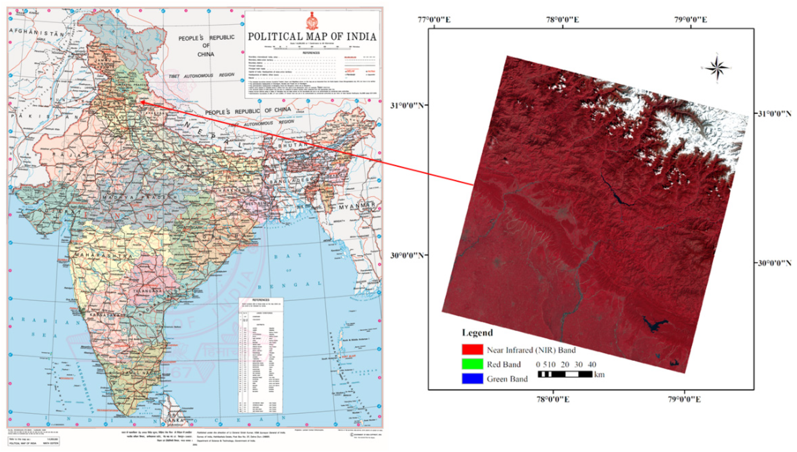
The study area lies between longitudes 77°34′43″ E to 78°18′22″ E and latitudes 29°56′22″ N to 31°02′53″ N. The place has a moderate climate, as it is located at Himalayan foothills. Temperatures in summer are not very high, but during winters they can even reach below the freezing point. In summers, the temperature range is around 16.7–36 °C, whereas in winters it decreases to 5.2–23.4 °C. The scene extent and geographic location of the study area is shown in Figure 1. The vegetation cover is highlighted in the red color of the false-color composite (FCC) image of the study area. The FCC image (Figure 1) for the study area was generated with an infrared, red, and green band of the Landsat 8 data, which was acquired on 2 October 2018. Dry riverbeds and urban settlements are highlighted in cyan color in the FCC. Dry riverbeds could be easily identified in the study area as linear features. The water body is appearing as dark blue color and the agricultural fields are shown in light red homogeneous patches. The snow cover over the Himalayan region is visible in white color in the North East region of the FCC image of Figure 1.
3. Methodology for LST Estimation
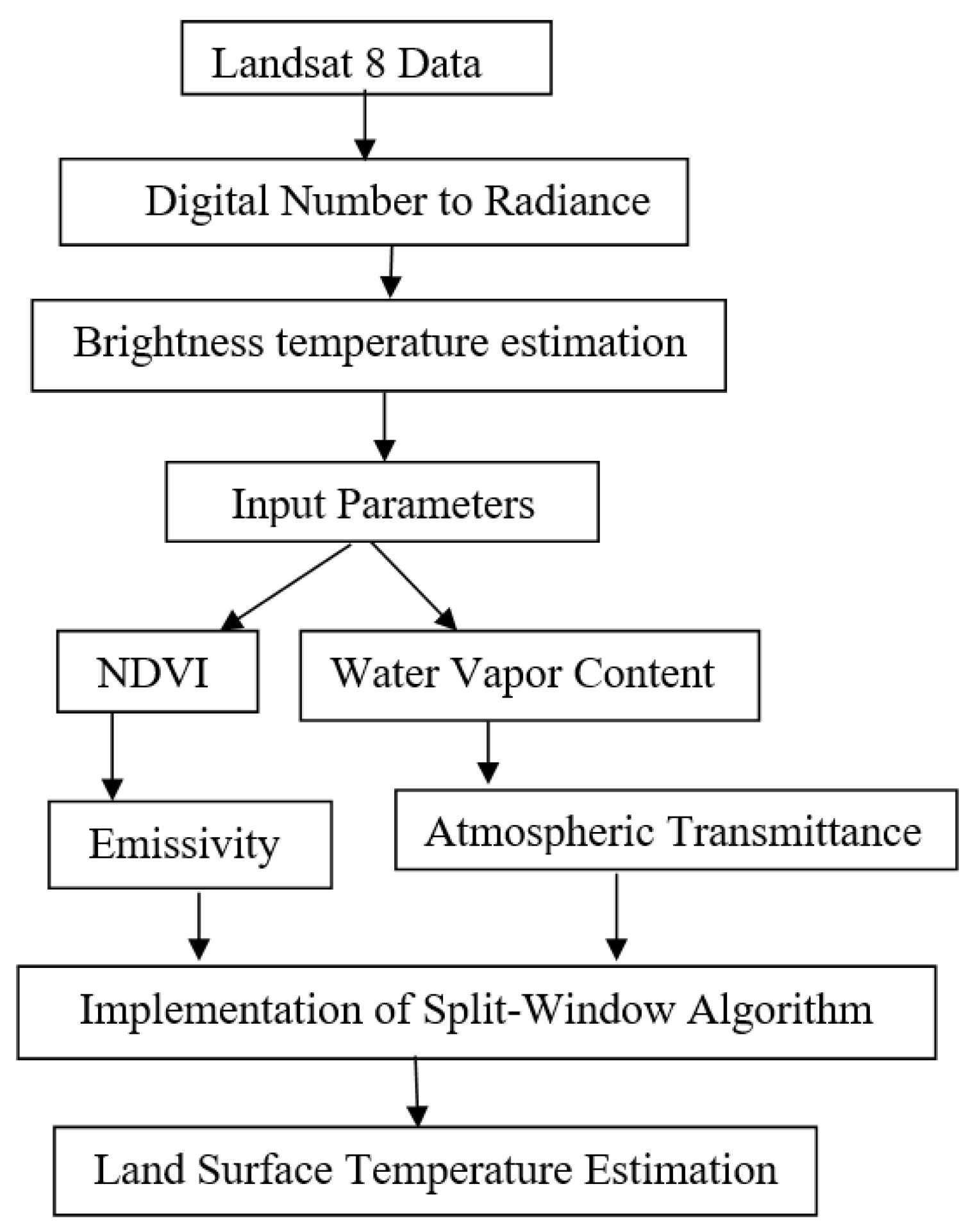
The methodological steps for LST estimation are shown in Figure 2. The first step of the methodology involves the Digital Number (DN) to radiance conversion. The brightness temperature was calculated using Equation (1) [14].
where and are constants, their values provided in the metadata file, or user manual, is the spectral radiance calculated using the given Equation (2).
Here, is the multiband radiance and is the add-band radiance, both of them provided in the image Metadata. is the digital number.
The split-window algorithm has been used for the calculation of LST. To eliminate the atmospheric contribution, the split-window algorithm takes into account the differential absorption of water vapor between two adjacent channels. The channels are centered on 11.0 and 12 µm respectively. It has been proven that the general split window algorithm could accurately determine the LST, but the errors occur mainly due to perceptible water vapor and emissivity. Atmospheric transmittance and land surface emissivity were the only two required parameters. Due to the accuracy and simplicity of the estimation process for input parameters, Qin et al.’s algorithm was applied to thermal infrared sensor (TIRS) data [14,15,16]. The equation used in the split-window algorithm to calculate surface temperature is shown in Equation (1) [14,17].
Here, is the LST, and are the brightness temperatures for band 10 and band 11, respectively. and are the three coefficients that are obtained by emissivity and atmospheric transmittance for both of the TIRS bands, with the use of Equation (4)
The parameters used in the above set are derived with the help of Equation (5).
Here, is the emissivity, is the atmospheric transmittance, and ‘i’ denotes the band number [15].
3.1. Emissivity
Emissivity is calculated using the NBEM (NDVI-based) method. For comparison purposes, another method—method of normalized emissivity of MNE—is also applied. The mathematical formula for MNE is given in Equation (6) [18].
Here, is the measured radiance, is the upwelling radiance and is the downwelling radiance, is the atmospheric transmittance, and is the blackbody radiance, which can be calculated using Equation (7) [14,16].
Here, and are constants with values 1.191∗ and , respectively. is the wavelength of band 10 and 11, and T is the maximum of brightness temperature.
3.2. Atmospheric Transmittance
There are several constituents present in the atmosphere. Water vapor, , and other gases are also a part. However, during an atmospheric correction, only water vapor is taken into consideration, because in the atmosphere, the contents of gases are more stable in comparison. Instead, the water vapor content has a high degree of variability, allowing the atmospheric transmittance to depend heavily on it [14]. The equations to calculate transmittance with the help of water vapor content (content range—0.5–3 g/cm²) are shown in Equation (8) [15].
where c0, c1, and c2 are coefficients. N is the number of adjacent pixels (excluding cloud pixels). and are brightness temperatures for the band i and j, respectively, at the TOA for the kth pixel, and w is the water vapor content. and are mean or median brightness temperatures for the N pixels for the two bands.
4. Results and Discussion
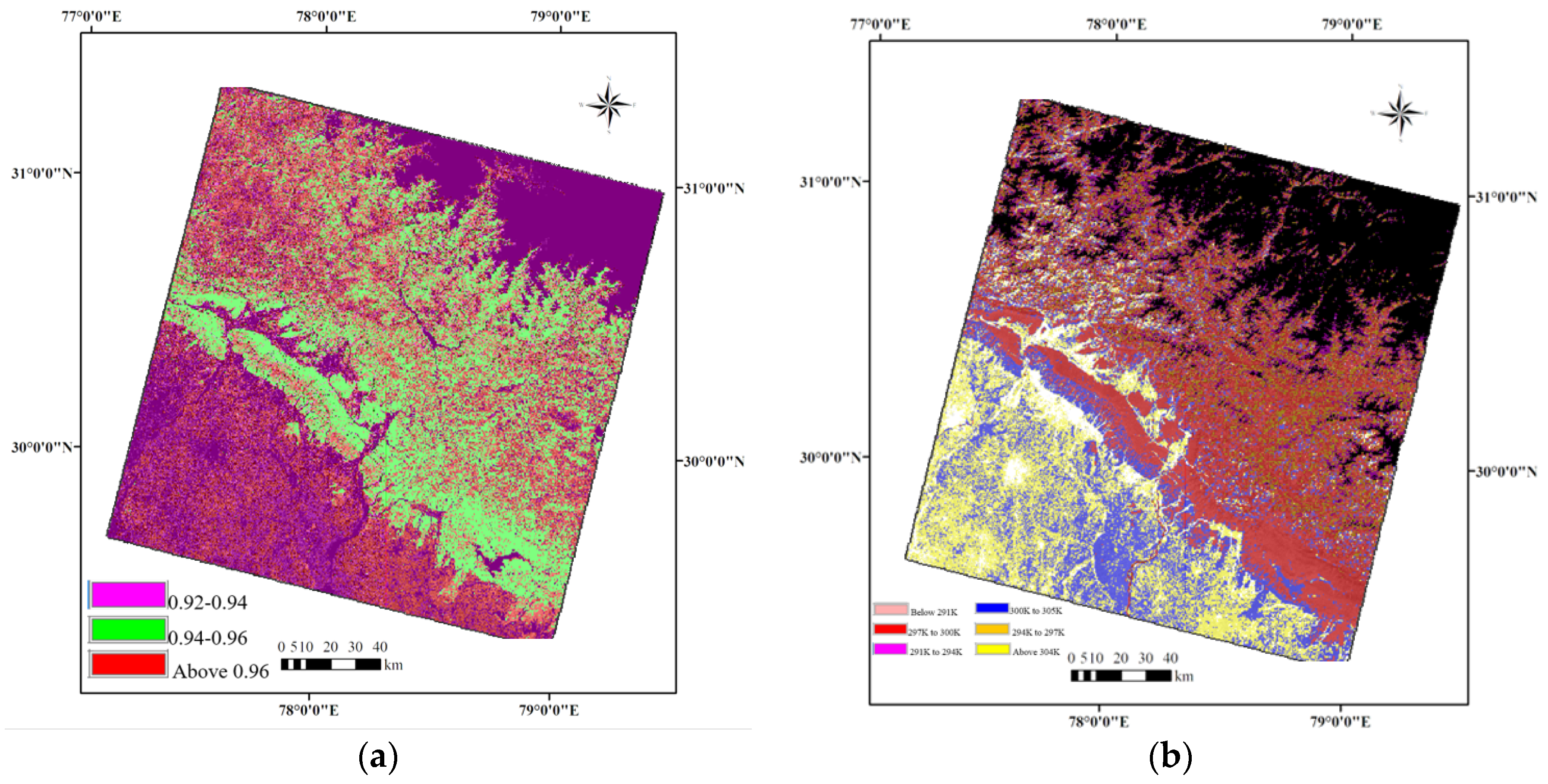
To determine land surface temperature, firstly brightness temperature is calculated for all of the images. The second step is to obtain the required parameters, which are emissivity and atmospheric transmittance. Lastly, the split-window algorithm is applied to the images. The emissivity image as shown in Figure 3a was generated for the Landsat data of October 15, 2017. The general value range for every studied image is observed to be about 0.91–0.97. This range indicates the presence of water and vegetation as it is proximate to 1.
After the retrieval of all essential parameters, the split-window algorithm is applied for four consecutive years of 2015, 2016, 2017, and 18. Split window incorporates the brightness temperature obtained from TIRS bands to retrieve LST. The accuracy of the split-window algorithm is more reliable due to implementation of atmospheric correction to retrieve LST. The LST values were retrieved for those scenes of LANDSAT-8 data for which the manmade and natural features were not covered by the cloud. Three images for the years 2015 to 2018 were selected as per the availability of the cloud-free data for September, October, and November. The LST map (Figure 3b) shows the very low temperature for snow-covered (black color) areas, and very high temperature (yellow color) is recorded for the urban area and the agricultural field. Manmade features like urban area and agricultural fields showed very high LST, and natural features like forest cover and water bodies showed moderate to low emissivity (Figure 3b).
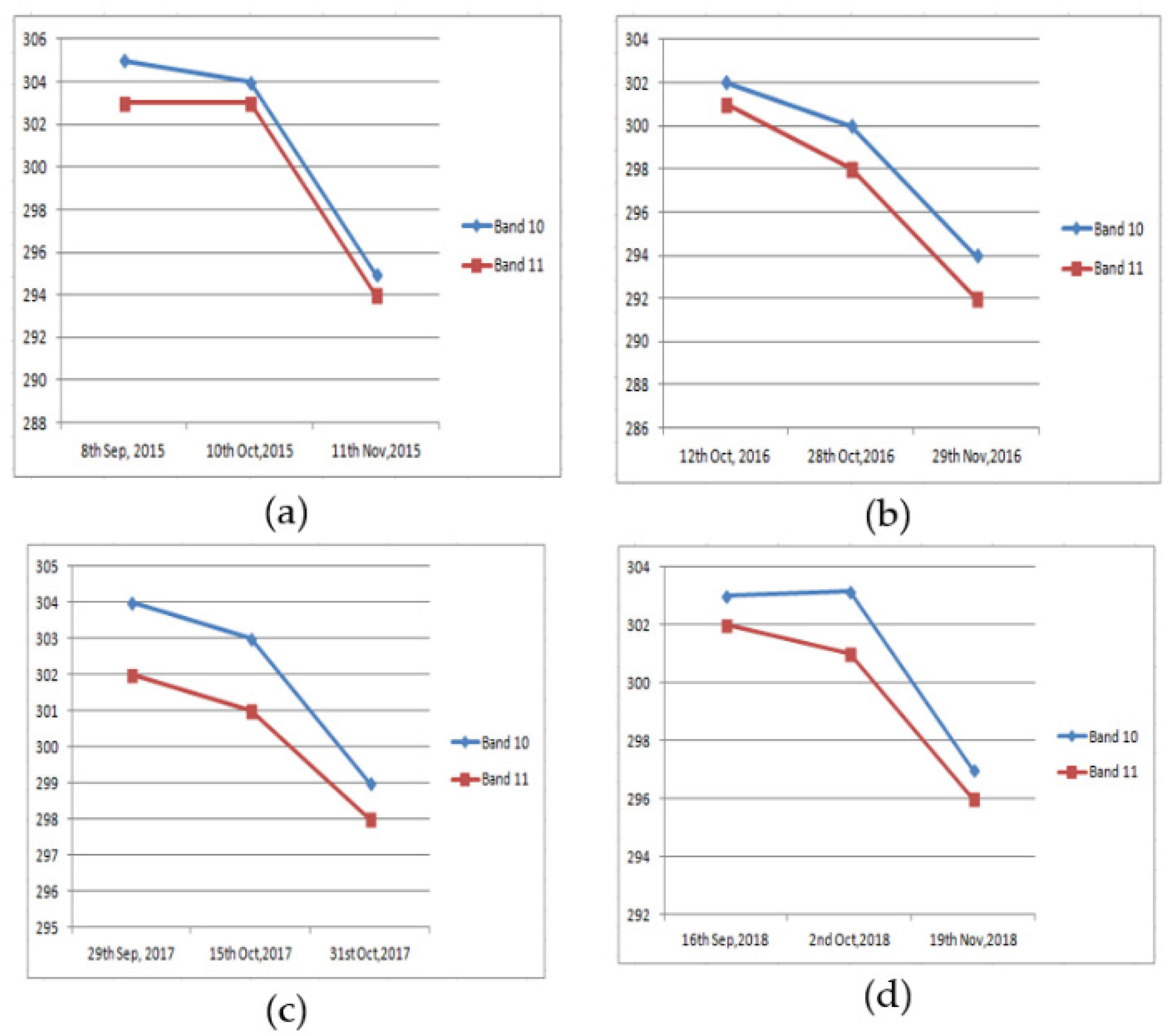
A temporal analysis of the maximum LST of the study area for TIRS bands 10 and 11 is shown in Figure 4. The months of September, October, and November face a gradual decrease in temperature. The first six months of year face gradual increase in the temperature because of the same reason of climate change and the approach of summer season. Additionally, if the land surface temperature for September, October, and November is observed over consecutive years, a very slight increase in temperature is seen. It could be easily seen from Figure 4 that the maximum LST was observed for the September month of the years 2015, 2016, and 2017, but in the band 10 for 2 October 2018, it was found that the LST is higher than September 2018. In comparison to the three months of the years, 2015 to 2018 LST value recorded for November month is always low. This increase in temperature is due to several factors that include manmade anthropogenic and climatic conditions. Effect of seasonal change on LST [19] could also be seen in Figure 4. September is a month of monsoon season in India, and November is the month of winter season. A fall in temperature has been observed from September to November, indicating the change in LST, which is due to the change in weather.
5. Conclusions
Land surface temperature is mandatory for the determination of various geophysical processes, including evapotranspiration and desertification. To derive the land surface temperature in this project, Landsat 8 images have been used. It is found that the split-window algorithm seems to be the most appropriate approach due to its simplicity and provision for atmospheric correction. The inverse relationship between the wavelength and temperature has also been proved with brightness temperature, and the land surface temperature is slightly increased for Band 10 as compared to Band 11. Atmospheric transmittance is a factor that causes disruption in the results of land surface temperature, and hence the split-window algorithm achieves accuracy by providing atmospheric correction for a given image.
Author Contributions
Conceptualization: S.K.; methodology: S.J.; formal analysis: S.J.; data curation: S.J.; writing—original draft preparation: S.J.; writing—review and editing: S.K.; visualization: S.J., S.K.; supervision: S.K. All authors have read and agreed to the published version of the manuscript.
Funding
This research received no external funding.
Acknowledgments
Authors are thankful to the USGS and MODIS team to provide Landsat 8 and atmospheric products to complete this project.
Conflicts of Interest
The authors declare no conflict of interest.
References
- Babu, A.; Kumar, S. SBAS interferometric analysis for volcanic eruption of Hawaii island. J. Volcanol. Geotherm. Res. 2019, 370, 31–50. [Google Scholar] [CrossRef]
- Kumar, S.; Garg, R.D.; Govil, H.; Kushwaha, S.P.S. PolSAR-Decomposition-Based Extended Water Cloud Modeling for Forest Aboveground Biomass Estimation. Remote Sens. 2019, 11, 2287. [Google Scholar] [CrossRef]
- Asopa, U.; Kumar, S. UAVSAR Tomography for Vertical Profile Generation of Tropical Forest of Mondah National Park, Gabon. Earth Space Sci. 2020, 7, e2020EA001230. [Google Scholar] [CrossRef]
- Shafai, S.S.; Kumar, S. PolInSAR Coherence and Entropy-Based Hybrid Decomposition Model. Earth Space Sci. 2020, 2020, e2020EA001279. [Google Scholar] [CrossRef]
- Singh, A.; Gaurav, K.; Meena, G.K.; Kumar, S. Estimation of Soil Moisture Applying Modified Dubois Model to Sentinel-1; A Regional Study from Central India. Remote Sens. 2020, 12, 2266. [Google Scholar] [CrossRef]
- Chaudhary, V.; Kumar, S. Marine Oil Slicks Detection using Spaceborne and Airborne SAR data. Adv. Space Res. 2020, 66, 854–872. [Google Scholar] [CrossRef]
- Awasthi, S.; Thakur, P.K.; Kumar, S.; Kumar, A.; Jain, K.; Mani, S. Snow Density retrieval using Hybrid polarimetric RISAT-1 datasets. IEEE J. Sel. Top. Appl. Earth Obs. Remote Sens. 2020, 13, 3058–3065. [Google Scholar] [CrossRef]
- Voogt, J.A.; Oke, T.R. Thermal remote sensing of urban climates. Remote Sens. Environ. 2003, 86, 370–384. [Google Scholar] [CrossRef]
- Weng, Q.; Lu, D.; Schubring, J. Estimation of land surface temperature-vegetation abundance relationship for urban heat island studies. Remote Sens. Environ. 2004, 89, 467–483. [Google Scholar] [CrossRef]
- Gillespie, A.; Rokugawa, S.; Matsunaga, T.; Steven Cothern, J.; Hook, S.; Kahle, A.B. A temperature and emissivity separation algorithm for advanced spaceborne thermal emission and reflection radiometer (ASTER) images. IEEE Trans. Geosci. Remote Sens. 1998, 36, 1113–1126. [Google Scholar] [CrossRef]
- Guha, S.; Govil, H.; Gill, N.; Dey, A. A long-term seasonal analysis on the relationship between LST and NDBI using Landsat data. Quat. Int. 2020. [Google Scholar] [CrossRef]
- Li, Z.-L.; Tang, B.-H.; Wu, H.; Ren, H.; Yan, G.; Wan, Z.; Trigo, I.F.; Sobrino, J.A. Satellite-derived land surface temperature: Current status and perspectives. Remote Sens. Environ. 2013, 131, 14–37. [Google Scholar] [CrossRef]
- Wang, M.; He, G.; Zhang, Z.; Wang, G.; Wang, Z.; Yin, R.; Cui, S.; Wu, Z.; Cao, X. A radiance-based split-window algorithm for land surface temperature retrieval: Theory and application to MODIS data. Int. J. Appl. Earth Obs. Geoinf. 2019, 76, 204–217. [Google Scholar] [CrossRef]
- Qin, Z.; Dall’Olmo, G.; Karnieli, A.; Berliner, P. Derivation of split window algorithm and its sensitivity analysis for retrieving land surface temperature from NOAA-advanced very high resolution radiometer data. J. Geophys. Res. Atmos. 2001, 106, 22655–22670. [Google Scholar] [CrossRef]
- Du, C.; Huazhong, R.; Qin, Q.; Meng, J.; Zhao, S. A Practical Split-Window Algorithm for Estimating Land Surface Temperature from Landsat 8 Data. Remote Sens. 2015, 7, 647–665. [Google Scholar] [CrossRef]
- Qin, Z.; Karnieli, A.; Berliner, P. A mono-window algorithm for retrieving land surface temperature from Landsat TM data and its application to the Israel-Egypt border region. Int. J. Remote Sens. 2001, 22, 3719–3746. [Google Scholar] [CrossRef]
- Qin, Z.; Xu, B.; Zhang, W.; Li, W.; Chen, Z.; Zhang, H. Comparison of split window algorithms for land surface temperature retrieval from NOAA-AVHRR data. In Proceedings of the IGARSS 2004, 2004 IEEE International Geoscience and Remote Sensing Symposium, Anchorage, AK, USA, 20–24 September 2004; Volume 6, pp. 3740–3743. [Google Scholar]
- Beatriz, S.; Rolim, A.; Grondona, A.; Hackmann, C.L.; Rocha, C. A Review of Temperature and Emissivity Retrieval Methods: Applications and Restrictions. Am. J. Environ. Eng. 2016, 6, 119–128. [Google Scholar]
- Guha, S.; Govil, H. Seasonal impact on the relationship between land surface temperature and normalized difference vegetation index in an urban landscape. Geocarto Int. 2020, 37, 2252–2272. [Google Scholar] [CrossRef]
Figure 1.
Location of the study area in the map of India released by the Survey of India and a false-color composite image of the Landsat 8 data.
Figure 1.
Location of the study area in the map of India released by the Survey of India and a false-color composite image of the Landsat 8 data.

Figure 2.
Methodological flow diagram for LST estimation.

Figure 3.
Landsat 8 image-based (a) emissivity (b) LST for the study area for 15 October 2017.

Figure 4.
Maximum LST for the years (a) 2015; (b) 2016; (c) 2017; (d) 2018.

Publisher’s Note: MDPI stays neutral with regard to jurisdictional claims in published maps and institutional affiliations. |
© 2020 by the authors. Licensee MDPI, Basel, Switzerland. This article is an open access article distributed under the terms and conditions of the Creative Commons Attribution (CC BY) license (https://creativecommons.org/licenses/by/4.0/).
Share and Cite
MDPI and ACS Style
Jain, S.; Kumar, S. Spaceborne Thermal Remote Sensing for Characterization of the Land Surface Temperature of Manmade and Natural Features. Proceedings 2020, 67, 2. https://0-doi-org.brum.beds.ac.uk/10.3390/ASEC2020-07568
AMA Style
Jain S, Kumar S. Spaceborne Thermal Remote Sensing for Characterization of the Land Surface Temperature of Manmade and Natural Features. Proceedings. 2020; 67(1):2. https://0-doi-org.brum.beds.ac.uk/10.3390/ASEC2020-07568
Chicago/Turabian StyleJain, Sakshi, and Shashi Kumar. 2020. "Spaceborne Thermal Remote Sensing for Characterization of the Land Surface Temperature of Manmade and Natural Features" Proceedings 67, no. 1: 2. https://0-doi-org.brum.beds.ac.uk/10.3390/ASEC2020-07568