Adaptive Water Sampling Device for Aerial Robots


Department of Agricultural Sciences, Clemson University, Clemson, SC 29634, USA
*
Author to whom correspondence should be addressed.
Drones 2020, 4(1), 5; https://0-doi-org.brum.beds.ac.uk/10.3390/drones4010005
Submission received: 23 January 2020
/
Revised: 30 January 2020
/
Accepted: 3 February 2020
/
Published: 6 February 2020
(This article belongs to the Special Issue Fundamental and Applied Research in Unmanned Aircraft Systems Technology)
Abstract
:Water quality monitoring and predicting the changes in water characteristics require the collection of water samples in a timely manner. Water sample collection based on in situ measurable water quality indicators can increase the efficiency and precision of data collection while reducing the cost of laboratory analyses. The objective of this research was to develop an adaptive water sampling device for an aerial robot and demonstrate the accuracy of its functions in laboratory and field conditions. The prototype device consisted of a sensor node with dissolved oxygen, pH, electrical conductivity, temperature, turbidity, and depth sensors, a microcontroller, and a sampler with three cartridges. Activation of water capturing cartridges was based on in situ measurements from the sensor node. The activation mechanism of the prototype device was tested with standard solutions in the laboratory and with autonomous water sampling flights over the 11-ha section of a lake. A total of seven sampling locations were selected based on a grid system. Each cartridge collected 130 mL of water samples at a 3.5 m depth. Mean water quality parameters were measured as 8.47 mg/L of dissolved oxygen, pH of 5.34, 7 µS/cm of electrical conductivity, temperature of 18 °C, and 37 Formazin Nephelometric Unit (FNU) of turbidity. The dissolved oxygen was within allowable limits that were pre-set in the self-activation computer program while the pH, electrical conductivity, and temperature were outside of allowable limits that were specified by Environmental Protection Agency (EPA). Therefore, the activation mechanism of the device was triggered and water samples were collected from all the sampling locations successfully. The adaptive water sampling with Unmanned Aerial Vehicle-assisted water sampling device was proved to be a successful method for water quality evaluation.
1. Introduction
Monitoring water quality is important to determine the impact of contaminants from agriculture, stormwater, wastewater, and residential houses. According to The United Nations World Water Development Report, 80% of wastewater in the world is released to the rivers, lakes, and oceans without adequate treatment [1]. More than 3.4 million people die from water-related diseases every year [2]. Polio, malaria, cholera, and diarrhea are some of the major waterborne diseases responsible for causing health threats [3]. World Health Organization (WHO) issues guidelines for water quality to ensure the safety of drinking water to protect public health in developed and developing countries [4]. United States Centers for Disease Control and Prevention (CDC) reports that 780 million people do not have access to clean water sources worldwide [5].
Determining the impacts of climate change and environmental pollution on ecologically sensitive, large, and remote waterbodies is difficult because of the complex dynamics of water quality monitoring, high costs, and extensive analyses of diverse data sets [6,7,8,9,10]. Therefore, innovative approaches for water quality monitoring are necessary to enhance water quality evaluation and to prevent waterborne diseases and deaths.
Water quality monitoring involves analyses and evaluation of water properties in freshwater sources to ensure that the water source provides safe water for drinking, irrigation, and livestock production. Quantitative and qualitative assessment of water quality parameters include dissolved oxygen (DO), pH, electrical conductivity (EC), salinity, temperature, turbidity, water depth, algal chlorophyll content, total phosphorus, nitrogen, and suspended solids [11,12]. Low concentration of DO, temperature, salinity, and pH in addition to increased levels of nitrogen, total phosphorus, turbidity, and algal chlorophyll indicate poor water quality which affect the rate of biological and chemical activities in water [13,14,15]. In situ or on site measurements of these parameters can be used for the rapid evaluation of water quality. If the measured parameters are not within the allowed limits, water samples can be collected for further laboratory analysis.
Water sample collection from lakes and ponds are often based on manual sampling from shore or with a boat mostly by volunteers [16]. Manual water sampling from difficult to access lakes, retired mining zones, or water bodies that are surrounded by steep and difficult terrain may be dangerous. In addition, lakes with cyanobacteria blooms increases health risks to humans during water sampling [17].
Water quality monitoring stations and wireless sensor networks are installed in water bodies to monitor water quality [13]. These stations continuously assess water quality by making in situ measurements over a long period [18,19]. The continuously measured water quality parameters are transmitted to a monitoring center or a web server to enable data storage and online access [20]. However, water quality stations may provide unreliable data due to continuously used sensors requiring regular maintenance [21,22]. As the sensor stations are at fixed locations, they provide water quality data with relatively low spatial resolutions. All of these methods are time-consuming, spatially limited, costly, or difficult to deploy at multiple locations. In addition to fixed water quality monitoring stations and networks, remotely controlled watercrafts that can either operate on the water surface or underwater have been developed [23,24,25,26,27,28,29]. These watercrafts are controlled either manually by a remote controller or with integrated autonomous guidance systems. The water quality maps are created with spatially interpolated water quality data for visualization [30].
Recent studies investigated the use of remote sensing on water quality monitoring [31,32,33,34,35]. Among remote sensing platforms, Unmanned Aerial Vehicles (UAV) are being investigated in use of disaster relief operations, topo-bathymetric monitoring, and algal bloom monitoring of the surface waters [36,37,38]. Remote sensing can detect important visual changes in the environment but detecting pollutions and change in water quality parameters might be challenging [37,39,40]. In addition to remote sensing, in situ water quality measurement with UAV integrated sensor systems was tested for water quality monitoring [41,42,43,44]. However, monitoring surface water environments require physical water samples that are taken at specific depths for intended water quality analysis [45,46]. The physical water samples are required for accuracy evaluation of water quality predictions that were driven based on remote sensing [40].
UAVs provide unique opportunities for remote water sample collection from surface waters. UAVs can remotely access a waterbody for physical water sample collection to better understand the distribution and extent of contaminants [35,47,48]. The UAV-mounted water samplers can be submerged to a specific depth with additional subsystems to analyze depth-specific water quality parameters [49]. An example application of a UAV-mounted water sampler is the sample collection from mines and pit lakes, and isolated multiple waterbodies [50,51,52]. Using a UAV for water sampling is generally limited by the payload and endurance capacity to carry water samples from desired locations to the shore [53]. In addition, these systems were designed to collect water samples from waterbodies without making in situ measurements of water quality parameters. Unnecessary water sampling could be eliminated to reduce water sample analysis costs by using an adaptive water sampler that measures the major water quality parameters before sample collection [54,55,56]. The adaptive water samplers continuously monitor changes in water quality parameters and capture water samples when the conditions were satisfied [57]. The decision to collect water samples can be based on the allowable limits of water quality parameters or the limits of selected water quality parameters of interest [58]. Current adaptive water sampling systems are not compatible with UAV systems with limited payload and endurance capacity. Therefore, there is a need for a light-weight, robust, and UAV compatible adaptive water sampling systems. In order to address above challenges and to contribute to the current research, two separate in situ water quality measurement [44] and water sampling systems [48] were integrated with a single UAV and tested in an agricultural pond [59].
The objective of this research was to develop, test, and integrate a UAV compatible adaptive water sampling system for water quality evaluation of surface waters. The developed adaptive water sampling system reported in Koparan, Koc, Privette and Sawyer [59] was further improved by integrating turbidity and depth sensors while including self-activation in a mission flight.
2. Materials and Methods
2.1. UAV and Sensor Components for Adaptive Water Sampling
A custom-designed UAV was used for adaptive water sampling experiments [59]. Details regarding the payload capacity, endurance, and the autonomous water sampling performance of UAV were previously reported in Koparan et al. [59]. The adaptive water sampling approach utilizes water sampling cartridges and sensor array called the Water Sampling Device (WSD). The sensor node measurements were used for self-activation of the cartridges to collect water samples. The adaptive water sampling approach was intended to collect water samples when the measurements exceed allowable water quality limits, as well as record the in situ measurements for on site rapid water quality evaluation. A turbidity sensor and pressure sensor were integrated with the sensor node on WSD.
2.1.1. Turbidity Sensor Integration with the Sensor Node and Accuracy Assessment
The turbidity sensor was an attenuation type sensor that measures the loss of light between a light source and a detector that are placed at 180° (DFRobot, Pudong, Shanghai, China). The turbidity sensor detects suspended particles in water by measuring the light transmittance and scattering rate which varies depending on the concentration of total suspended solids (TSS) [21]. As these sensors work on the attenuation light principle, ambient light may affect the turbidity measurements [60]. Turbidity units can be reported as Formazin Nephelometric Units (FNU), Nephelometric Turbidity Unit (NTU), or Formazin Attenuation Unit (FAU). While these units may vary based on the instruments used, they have no standardized value and they are qualitative measurements [61]. The turbidity measurements that were made with light-attenuation-based turbidity sensors are not considered valid for explaining the actual turbidity levels in waters by most agencies. However, attenuation type sensors can be utilized to evaluate water clarity and monitor change in turbidity over time in surface waters [60]. Turbid water does not necessarily indicate an issue related to water quality but a change in turbidity may indicate the development of algal blooms or a change in suspended sediments in a lake.
A case was designed and 3D printed for the turbidity sensor in order to minimize ambient light interference. This case included two chambers and water passage channels that allowed water entry to where the sensor could measure turbidity while blocking the ambient light (Figure 1). An accuracy assessment was made in lab conditions to evaluate if the sensor provided reliable turbidity measurements when the sensor when housed in the case.
Calibration and accuracy assessments of the turbidity sensor were made using a formazin standard solutions at 25 °C [61]. The standard solutions had 62.5, 250, 1000, and 2000 FNU. These solutions were chosen for calibration because they mimic the typical minimum and maximum turbidity levels in lakes [58]. First, the sensor voltage values (0–5 V) were mapped to FNU turbidity levels in order to determine sensor’s response to a turbid solution. Second, a calibration equation was developed between the known turbidity and voltage response from the sensor measurements. Finally, the developed calibration equation was used in the microcontroller program to determine the turbidity water samples.
The turbidity sensor measurements were correlated with standard turbidity solutions to determine the measurement accuracy. Thirty continuous measurements were made in each standard turbidity solution and the data was retrieved from Arduino Integrated Development Environment (IDE). The average of the repeated 30 measurements were recorded as single trial. There were 24 trials in total because six repeated random turbidity measurements were made in the same standard solution to minimize operator errors. Last, the random measurements were compared with the standard turbidity values. Paired t-test analysis was conducted to determine if there is a significant difference between the turbidity sensor measurements and the standard solutions using the 0.05 level of significance.
2.1.2. Depth Sensor Integration with the Sensor Node and Accuracy Assessment
A previous work with the sensor node revealed the need for depth specific in situ water quality parameters [59]. A pressure sensor integration with the sensor node was made to provide accurate water quality parameter measurement at a specific water depth. The pressure sensor measures the water pressure and the microcontroller converts it into depth measurements. The conversion is made based on the principle that the water pressure increases by 1 atm with each 10 m of depth. The maximum measurement range of the pressure sensor was 10 m with a water depth resolution of 0.16 mm (Bar02, Blue Robotics, Torrance, CA, USA).
The pressure sensor and voltage converter circuit were placed in a 3D printed case and sealed with epoxy and painted for waterproofing (Figure 2). The pressure sensor was integrated with a microcontroller unit (Arduino, Atmel ATmega328P, San Jose, CA, USA). The microcontroller platform was placed on top of the UAV in a water-sealed box and the pressure sensor was suspended with a 3.5 m long tether.
Accuracy assessment of depth sensor was made using a 2 m tall clear tube filled with tap water. The depth sensor was lowered to random depths in the tube and depth measurements of the sensor were compared with the manual depth measurements. A correlation equation was developed from 19 depth measurements from the depth sensor and the actual depth. The pressure sensor was integrated with the sensor node as shown in Figure 3.
2.2. Evaluation of Sensor Node Stabilization Time
Sensors on the node required certain equilibrium time for accurate measurements. The equilibrium time is critical for the autonomous adaptive water sampling, because this timeframe determined how long the UAV stayed at each sampling location. Equilibrium time directly affected the battery usage of the UAV. The mission plan and self-activation program depended on equilibrium time information for decision making. Equilibrium time evaluation of DO, pH, EC, temperature, and turbidity were undertaken in 500 mL of tap water at room temperature (21 °C). The sensor node was fully submerged in the sample water. Commercially available multi parameter sensors (Sension 156 and HQ10, Hach, Loveland, CO, USA) were used along with the sensor node to determine how long it took for the sensor node to reach equilibrium. Sensor calibrations for both the sensor node and the commercial sensors were made according to the manufacturers’ specifications. Three repeated measurements were made with the commercial sensor to determine actual water quality parameters as reference measurements. Turbidity reference measurement was made with a turbidimeter (2100AN, Hach, Loveland, CO, USA). Continuous measurements were made with the sensor node for 5 min at 4 s intervals. The measurement intervals of 4 s were necessary in order to acquire measurements from all the sensors as specified by the manufacturers’ specifications. The equilibrium time of each sensor was recorded and examined.
2.3. Water Sampling Device Self-Activation and Test Procedure
The activation of the WSD was made based on the sensor node measurements. The decision for self-activation of WSD was made by the Micro Controller Unit (MCU) when the allowable limits of noncontaminant water quality indicators exceeded the limits. The allowable limits of selected water quality parameters were 6–12 mg/L for DO, 6.5–9.5 for pH, 100–2000 for EC, and 20–35 °C for temperature for lakes [62,63,64]. These allowable limits were introduced in the self-activation computer program and the WSD was set to initiate water collection when the sensor node measurements exceeded the programmed limits. Indoor measurements in the lab and outdoor experiments at the experiment site were conducted to test the performance of the self-activation mechanism of the WSD.
The indoor experiments were conducted for self-activation tests by placing the measurement probes in reference solutions and observing if the WSD was activated by the MCU or not. The probes for each sensor were randomly placed in individual reference solutions. These solutions ranged from below allowable limits to above allowable limits for each parameter to create different test conditions. Self-activation was tested at each solution and the WSD was reset after each trial. The probes were placed in tap water while one of the probes were placed in a standard solution during the trials. This provided within-the-limit measurements from other sensors to ensure that self-activation was achieved or not achieved based on the sensor that was in the standard solution. The self-activation trials for pH were conducted using pH standard solutions of 4, 7, and 10. The pH probe was placed in each solution randomly and self-activations were observed. It was expected that the WSD would be self-activated when the probe was placed in pH solutions of 4 and 10, since these values were outside of the allowable pH limits set in the computer program. It was expected that the WSD would not be self-activated when the probe was placed in pH solution of 7, since it was within the allowable limits. The self-activations while the probe was in the pH solutions of 4 and 10, and no self-activations while the probe was in the pH solution of 7 was recorded as successful trials. The trials with the self-activation decisions (i.e., triggering the sample collection when pH was 7 or not triggering the self-activation when pH solution was 4 or 10) were recorded as unsuccessful trials. The self-activation trials for EC were conducted using EC calibration solutions of 84 and 1413 µS/cm. The EC value of 84 µS/cm was used as a parameter that was outside the allowable limits, and EC value of 1413 µS/cm was used as a parameter that was within the allowable limits. The self-activation trials for DO were conducted using zero oxygen solution and tap water. The DO level of tap water was confirmed with a commercial DO meter. The zero oxygen solution was used as a parameter that was outside the allowable limits as low DO, and tap water was used as a parameter that was within the allowable limits. The self-activation trials for temperature were conducted in preheated tap water. The tap water of 500 mL placed in a beaker and it was preheated to 50 °C and probes were placed in it to acquire temperature measurements while the water was cooling. The beaker was placed in an ice bucket for cooling the sample down to 4 °C. Reference temperature measurements were made with a commercial temperature probe to confirm sensor node measurements. The temperature measurements below 25 °C and above 35 °C were used as parameters that were outside the allowable limits, and temperature measurements within 25 and 35 °C were used as parameters that were within the allowable limits.
2.4. Experiment Site
Lake Issaqueena is a man-made lake located in Pickens County, South Carolina. The US Environmental Protection Agency (EPA) classifies this lake as located in the Inner Southern Piedmont region. The lake basin is long and narrow with relatively steep shorelines. The lake covered approximately 36 ha while the total watershed is 3639 ha with a length of 13 km. The mean summer temperature is 21.9 °C while average winter temperature is 4 °C [65]. The widest section of the lake is approximately 400 m from shore to shore.
The South Carolina Department of Health and Environmental Control (SCDHEC) monitors water quality in Lake Issaqueena watershed with two stations. One of the stations was located on the Six Mile Creek (SV-205) which is the main surface water input for the Lake Issaqueena. The other monitoring station was located in the Lake Issaqueena (SV-360) however, the water quality monitoring at these stations ended in December 2005 due to compliance with water quality standards [66]. Lake Issaqueena was selected for adaptive water sampling experiments because experimental results could be compared with the historical data. In addition, new data sets could be produced for water quality evaluation at this station while testing the performance of the adaptive water sampling system. Lake Issaqueena is easily accessible and provides safe UAV flight conditions due to no boat access from the neighboring Keowee River. The UAV integrated WSD and the launch location are shown in Figure 4.
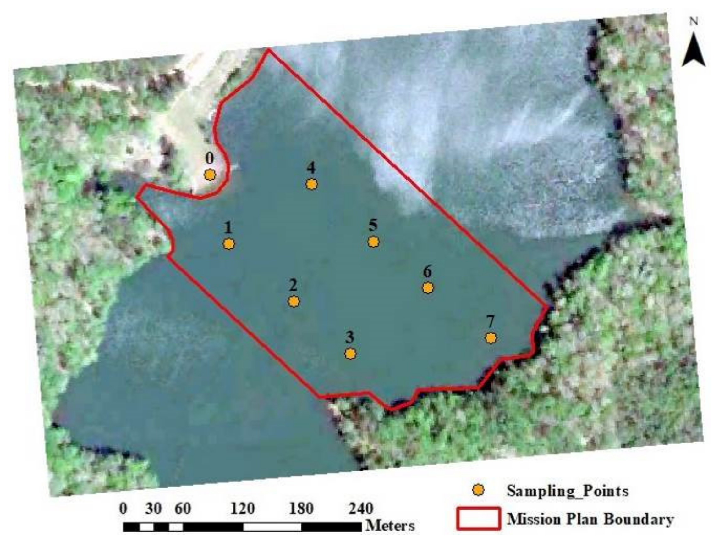
Adaptive sampling experiments were conducted at seven preselected locations in Lake Issaqueena. The locations were randomly selected at the center portion of the lake because the available battery power and endurance of the UAV limited the number of access points and maximum distance to be traveled [59]. Seven grid points were selected to enable maximum area coverage on the lake while testing the UAV for its maximum travel distance for safe flight. The sampling points were approximately 80 m apart from each other on the north east to south west row and approximately 90 m apart from each other on the northwest to south east row. The distance between launch point that was marked as 0 and the first sampling point was 73 m as it was the shortest flight distance. The distance between launch point and the seventh sampling point was 290 m as it was the longest flight distance. The launch location had a large open area that was free of trees and provided a flat surface for safe takeoff and landing. This location was the only available section at the lake to serve as a secure ground station. Due to this, the adaptive sampling trials were limited within the boundary that is shown in Figure 5.
2.5. Adaptive Water Sampling Data Collection
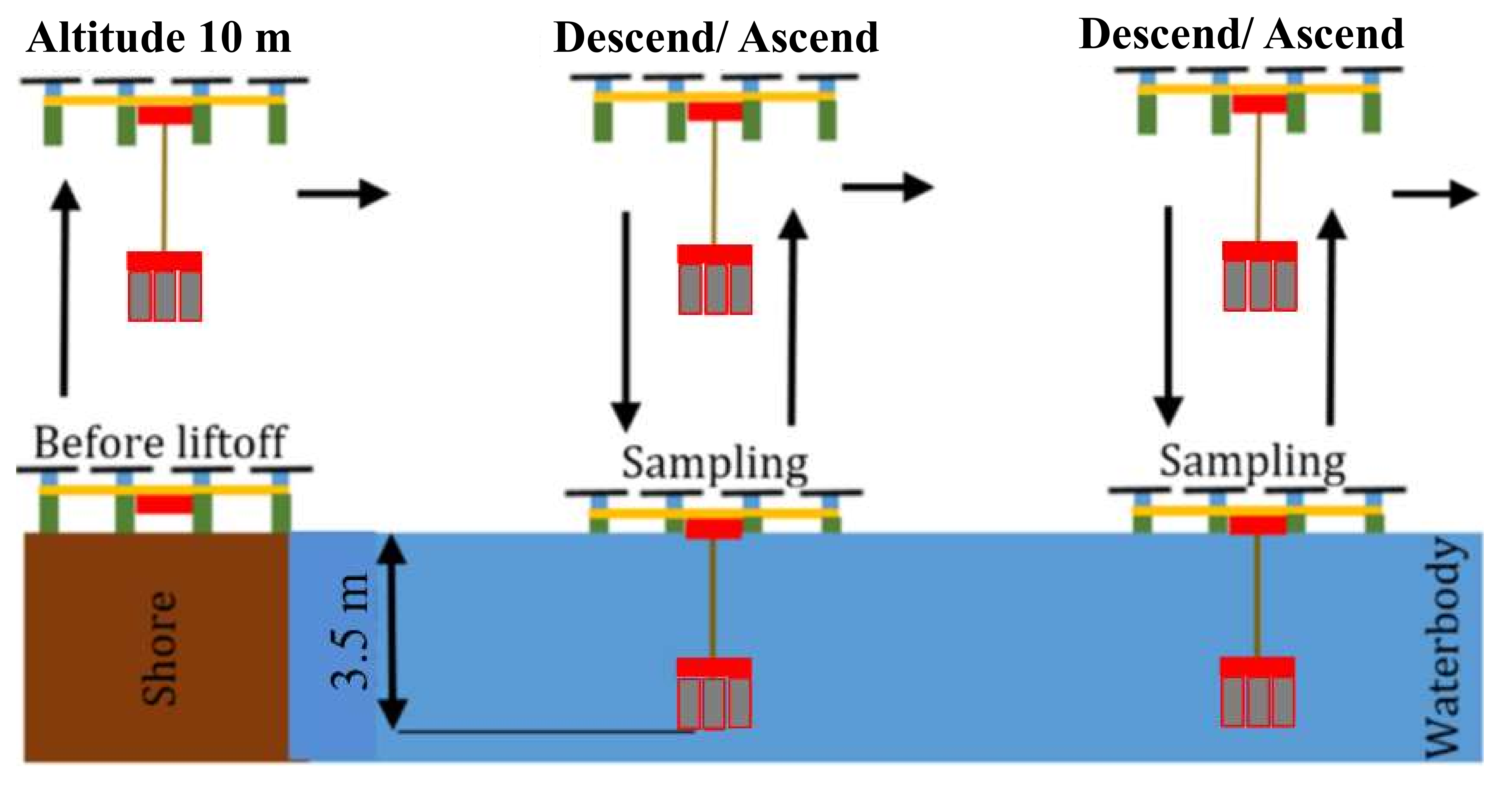
The experiment for adaptive water sampling was conducted on 9 May 2019, at 3 pm Eastern Time. UAV-assisted autonomous adaptive water sampling trials were conducted to test if the WSD would work at all times and collect 130 mL of water samples at each cartridge. The WSD was integrated with the UAV and was sent to predefined sampling locations with autonomous mission flights. The same mission plan boundary was chosen, and it was divided into individual mission plans due to long flight distances and battery limitations of the UAV. The locations 1, 2, and 3 were included in the first mission plan, locations 4, 5, and 6 were included in the second mission plan, and location 7 was included in the third mission plan. The adaptive water sampling depth was chosen as 3.5 m. Observations were made to ensure that UAV can land and take off with the WSD payload with captured water samples (Figure 6).
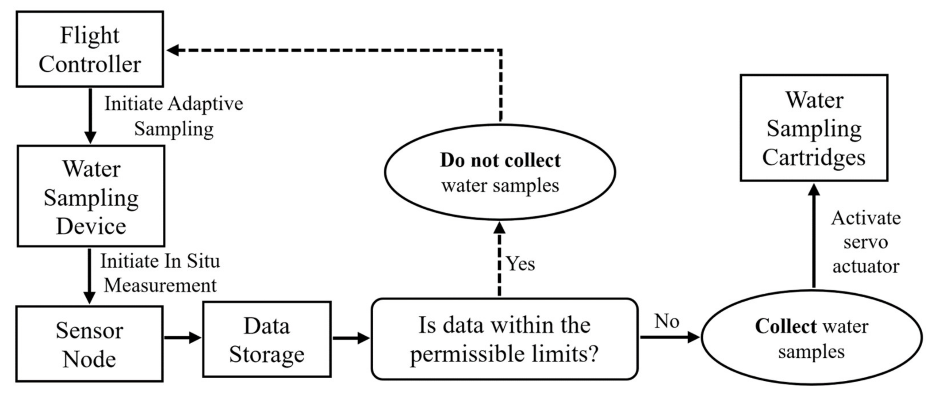
The WSD was designed as a subsystem that was integrated with the UAV. The initialization signal for adaptive sampling was acquired from the flight controller (Pixhawk, 3DR Robotics, Berkeley, CA, USA). The flight controller initiated the WSD as soon as the UAV reached the predefined sampling locations and landed on water surface. The MCU inside the WSD initiated the sensor node measurements and made water quality evaluations based on the allowable limits. Next, the WSD made decisions to either collect water samples when the measured parameters exceeded the allowable limits or did not collect water samples when the measured parameters remained within the allowable limits. The WSD self-activation decision is illustrated in Figure 7. The UAV returned to launch location after each self-activation trial for visual confirmation. If the self-activation was successful, the water samples were stored and marked by the location. Three replicate water samples were collected at each sampling location utilizing three cartridges in sequence. The collected water samples with the WSD were transported to the lab in plastic containers for turbidity analysis to compare the in situ turbidity sensor measurements with turbidimeter measurements (Supplementary Materials Video S1).
The collected water quality data was used to create maps for visualization of water quality distribution. The data was processed in ArcMap (Esri, Redlands, CA, USA) and interpolated using the Inverse Distance Weighted Interpolation (IDW) method [67]. Vector data in Geographic Information System (GIS) was interpolated to develop raster maps to simulate data values for intermediate locations.
3. Results and Discussion
3.1. Accuracy Evaluation of Depth and Turbidity Sensors
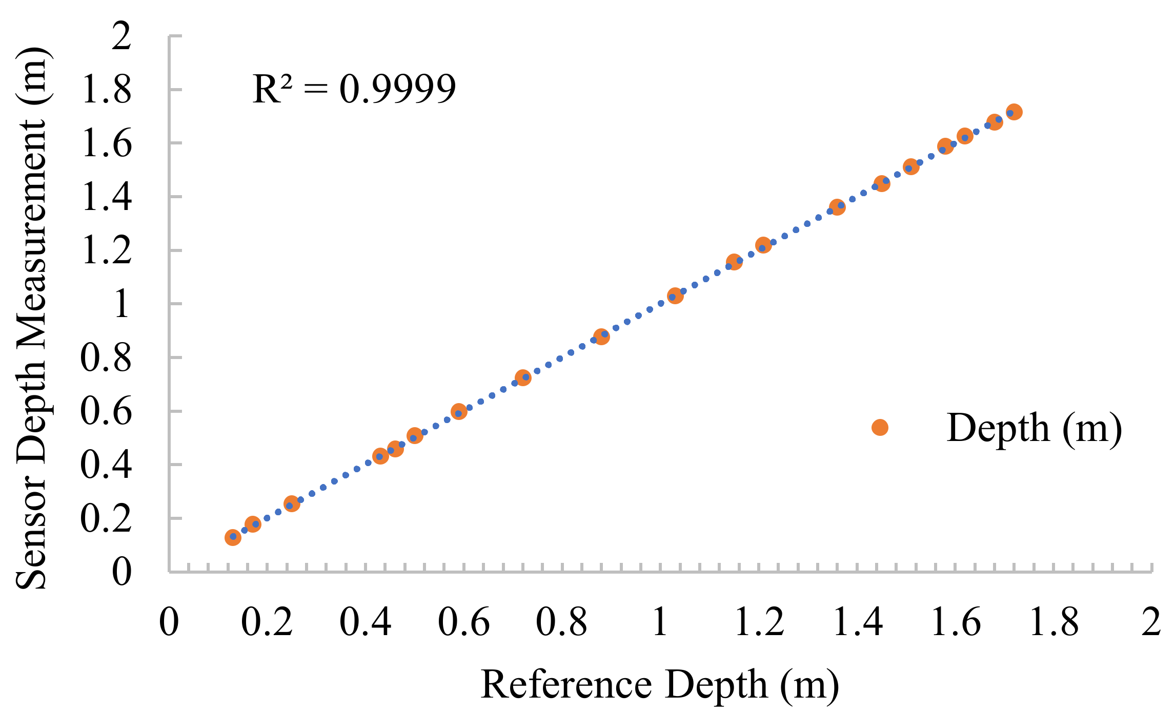
The depth measurements that were made indoor with the pressure sensor were identical when compared to the actual sensor depth (Figure 8). The 3D printed case for the pressure sensor prevented water from leaking and protected the circuits.
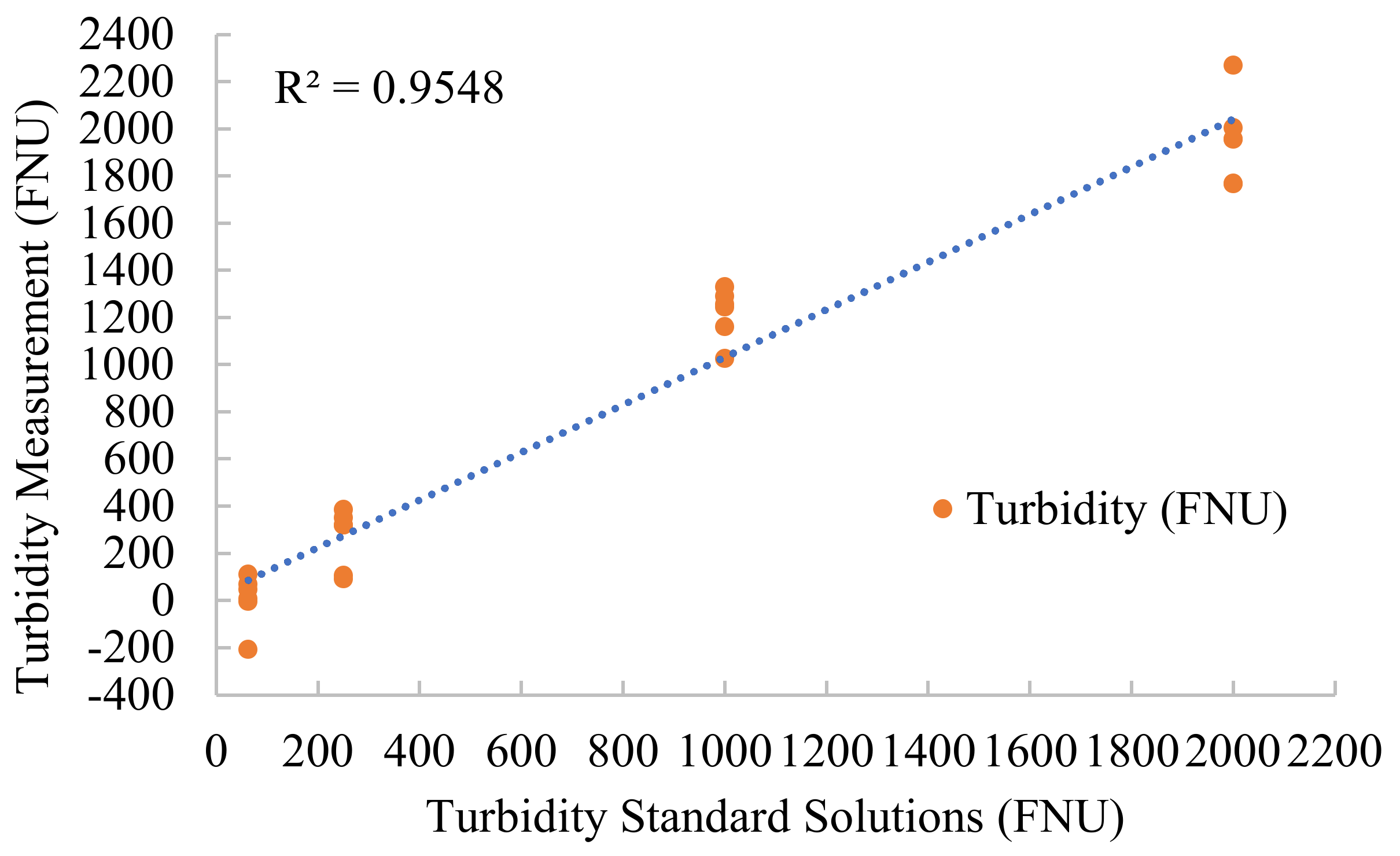
The accuracy assessment of turbidity by comparison with standard turbidity solutions showed that the turbidity sensor was reliable and could be used for outdoor experiments. The turbidity sensor measurements were 96% accurate when compared with the standard turbidity solutions of 62.5, 250, 1000, and 2000 FNU (Figure 9). The paired t-test showed that the mean difference between the turbidity sensor measurements and the standard solutions were not significant (t (23) = 0.89, p = 0.38). The mean difference was found to be 31 FNU. The mean turbidity measurements that were made in standard solutions by the sensor node were 859 FNU while the mean turbidity standard solution values were 828 FNU. The percent difference of the two mean turbidity values was 4%.
3.2. Evaluation of Sensor Node Equilibrium Time
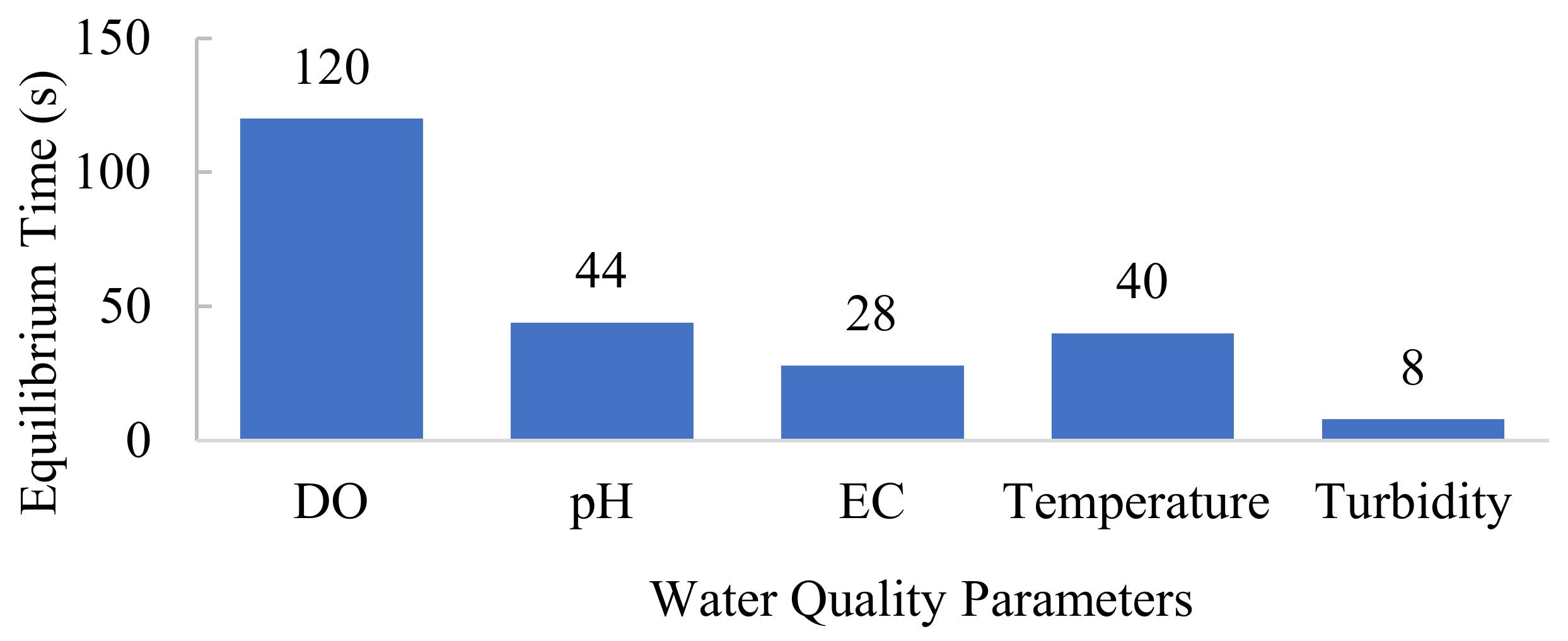
Preliminary experiments that were conducted to evaluate the equilibrium time of the sensor node revealed that the DO sensor took more time to reach equilibrium in comparison with other sensors (Figure 10). The turbidity sensor took the shortest time to reach equilibrium as 8 s while DO took 120 s. The DO values were always relatively higher than the actual DO values when the DO probe first entered the water samples. A sudden drop in the first 40 s and a steady decrease in DO values were typically observed. The equilibrium time for pH, EC, and temperature were 44, 28, and 40 s, respectively. The equilibrium time evaluation results showed that the sensor node had to be kept active for 120 s at each sampling location in order to make accurate measurements. The equilibrium time of 120 s was entered as a delay time in the mission plan. Once the UAV reached a sampling location, it waited for 120 s in idle mode to let the sensor node make measurements.
3.3. Self-Activation Trails of Adaptive Water Sampling
The WSD responded to sensor node measurements with 96% success rate during self-activation trials with known standard solutions. The total number of successful self-activations trials were recorded as 84 out of 88. The total number of unsuccessful self-activation trials were recorded as four (Video S2). The unsuccessful self-activations were random and independent from sensor type (Table 1). Repeated use of the WSD caused the servo to jitter and resetting the WSD after each trial solved the issue. The WSD was activated for water collection four seconds after the self-activation signal was sent by the MCU (Video S3). The four second timeframe appeared to be a processing delay, since the sensor node required four seconds to acquire measurement from individual sensors. This processing delay of four seconds was introduced in the mission plan to provide WSD enough time for water collection before takeoff.
3.4. Water Quality Evaluation of Lake Issaqueena and Adaptive Water Sampling
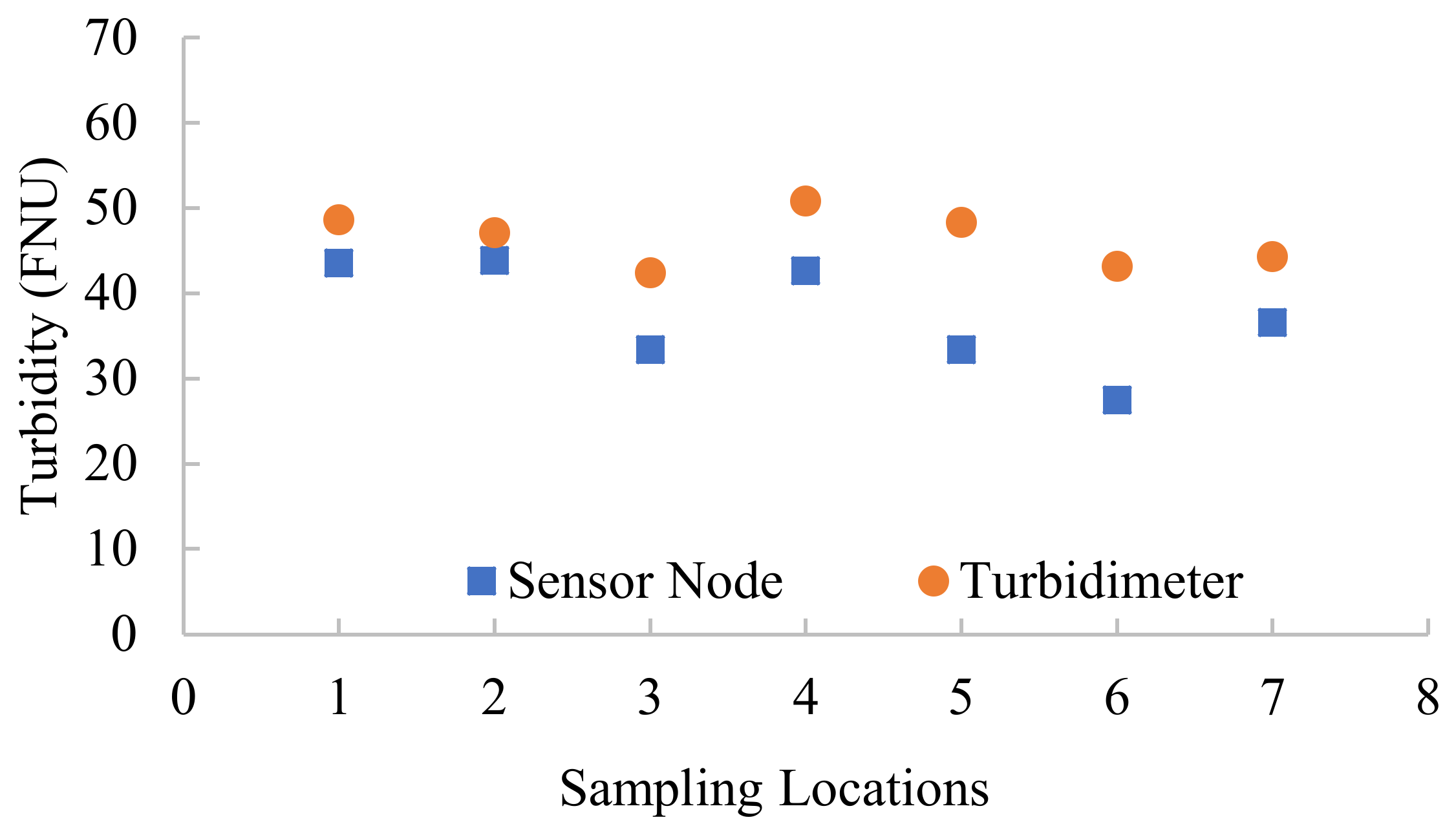
The turbidity measurements that were made with the sensor node from Lake Issaqueena and the turbidity measurements from the water samples showed a similar trend by location (Figure 11). The turbidity measurements were relatively close to each other when the range of turbidity levels in lakes were considered. However, mean difference in turbidity measurements between the sensor node and the turbidimeter appeared to be significant (t (6) = −5.17, p = 0.002). The mean differences in turbidity measurements were 9 FNU while the percent difference was 22%. Mean turbidity measurements made by the sensor node was 37 FNU while mean turbidity measurements made by the turbidimeter was 46 FNU.
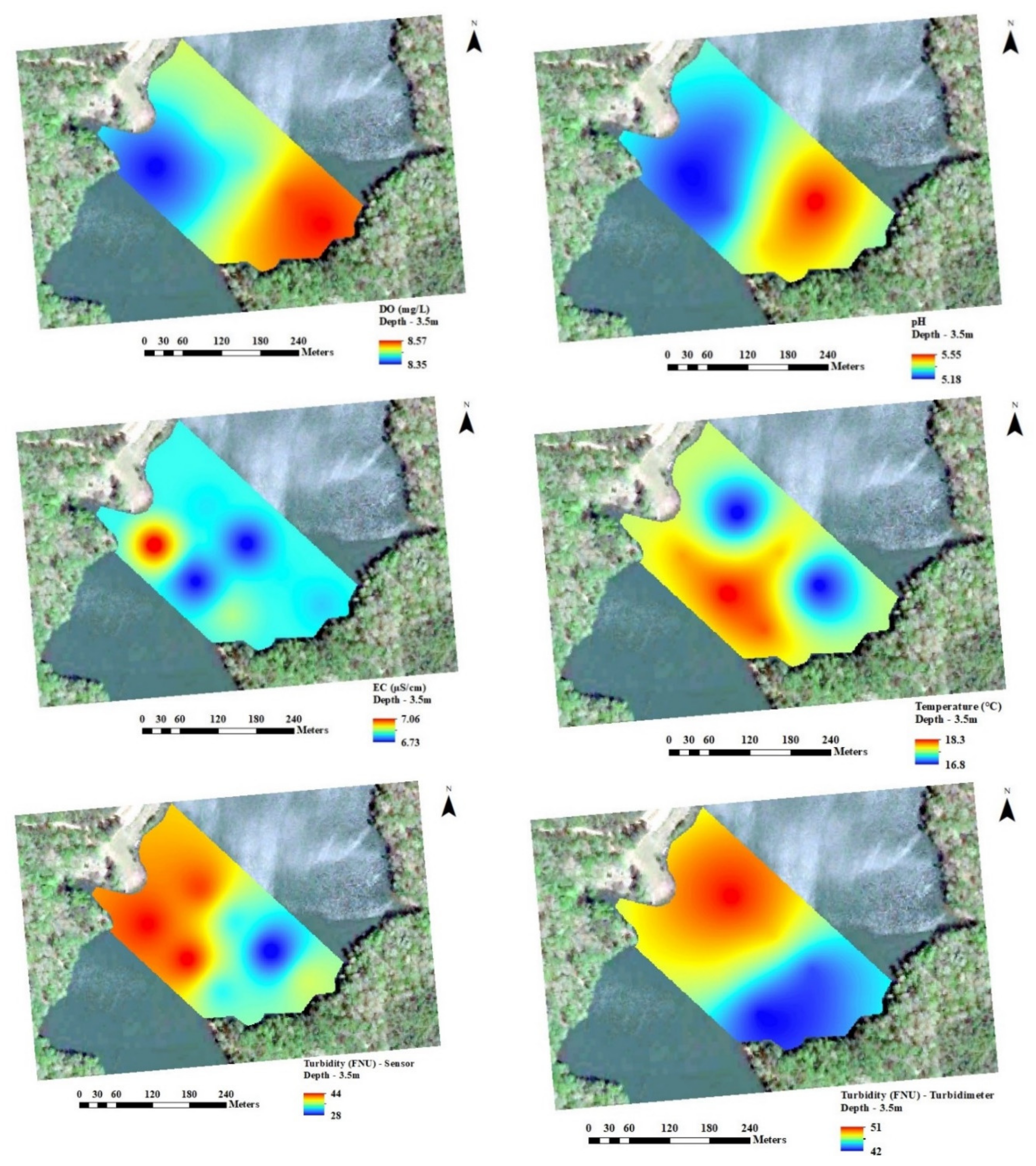
Turbidity units have no inherent value and they are qualitative measurements [61]. Turbidity measurements of these experiments were presented as water quality indicators based on clarity or transparency. The main factor that affected water transparency in the Lake Issaqueena was suspended sediment that was likely carried into the lake from the creek [60]. The turbidity maps that were created with both sensor node and turbidimeter measurements indicated high turbidity levels at the north west section of the sampling area in Lake Issaqueena (Figure 12). The increase in the turbidity at that section of the lake could be due to transport sediment carried by the stream after the rain event [68]. The turbidimeter measurements confirmed the high turbidity levels that were measured with the sensor node at the north west section of the lake. The difference in turbidity measurements between the sensor node and the turbidimeter was due to the ambient light that affected the turbidity measurements with an attenuation type sensor. However, the mean difference in the turbidity measurements was relatively small when compared to the natural range of turbidity in lakes. The overall turbidity in Lake Issaqueena ranged between 42 and 52 FNU based on turbidimeter results. The turbidity difference between the two shores of the lake was 9 FNU. Change in turbidity can indicate development of algal bloom or a steady increase in suspended sediment on the lake.
The adaptive water sampling experiments from the Lake Issaquena was successful at all locations. The UAV autonomously navigated to each sampling location, initiated WSD for in situ measurements, and stayed on the water surface for 120 s until the sensors reached equilibrium (Video S4). The in situ measurements indicated that the average pH, EC, and temperature measurements were below allowable limits (Table 2). The WSD was self-activated and captured three repeated 130 mL of water samples at all seven locations. The UAV successfully took off from the sampling locations and returned to the launch location with the collected water samples.
The lowest DO was 8.18 mg/L at sampling location one while the highest DO was 8.68 mg/L at sampling location six. The lowest pH was 4.98 at sampling location two while the highest pH was 5.92 at sampling location six. The average DO was 8.47 mg/L and the average pH was 5.34. The DO and pH were lower at the north west section within the boundary in the lake. Although the DO and pH did not change by larger numbers by location, their distribution was illustrated in maps with IDW interpolation (Figure 12). The maps illustrated the location where the stream water entered the waterbody and how the pH and DO changed.
The EC and water temperature were shown where the lowest and the highest values can be seen. Inverse distance weighting interpolation from in situ measurements did not show the small increments in the EC and temperature maps. The lowest EC was 6.49 µS/cm at sampling location five, while the highest EC was 7.52 µS/cm at sampling location one. The lowest water temperature was 16 °C at sampling location four, while the highest water temperature was 18.81 °C at sampling location two. The average EC was found as 7 µS/cm, and the average water temperature was found as 18 °C. The EC map showed that the EC was the highest where the stream makes entry to the waterbody. There was no clear pattern between stream water entry and its effect on water temperature, but the water temperature was higher at the south west section of the area.
4. Conclusions
Adaptive water sampling with UAV-integrated WSD proved to be an effective water quality evaluation method. The system made in situ measurements of DO, pH, EC, temperature, and turbidity with a precise sampling depth of 3.5 m and made the decision to collect water samples for lab analysis. Self-decision making to collect water samples based on in situ sensor node measurements were dependent on allowable limits of water quality parameters. The allowable limits of water quality parameters can be readjusted in the computer program for other types of water bodies, research interests, different climate conditions, and seasons. The size of the waterbody, sampling location, distance from the launch location, and the surroundings of the launch location are important parameters to consider adaptive water sampling with this type of aerial system.
A UAV of this size can accomplish safe water sampling at a maximum distance of 290 m. It is not recommended to operate the system for water sampling from a distance greater than 290 m because the UAV exceeds the line-of-sight limits and it becomes difficult to observe whether the UAV landed on water surface or it continues to fly. Piloting the UAV of this size at an approximate distance of 150 to 290 m requires a hand-free binocular to ensure landing and takeoff are achieved using the autopilot. Water quality parameters can be measured, and water samples can be collected for quick evaluations with this system within this distance in less than an hour. Rapid water sampling from various locations of a large water body provides valuable information about the type and the location of changes in the specific water quality parameters. Location-specific water quality information can help limnologists to identify a specific problem and develop appropriate management programs to prevent further potential contaminations. High-resolution water quality data can be acquired from difficult to access waterbodies and from waterbodies where no water quality monitoring stations exist. The UAV assisted adaptive water sampling system enables remote water quality monitoring without the need of entering a waterbody with a watercraft.
Supplementary Materials
The following videos are available online at the provided links. Video S1: Retrieval of water samples from the cartridges: https://www.youtube.com/watch?v=aDItCqGBOcE; Video S2: Water sampler was not activated due to within allowable limits measurements: https://www.youtube.com/watch?v=2MPv4MIZvtc; Video S3: Water sampler was activated due to exceeded allowable limits: https://www.youtube.com/watch?v=ss7g57C71yk; Video S4: Adaptive water sampling autonomous mission flight with the UAV: https://www.youtube.com/watch?v=Iij0evacUW8.
Author Contributions
Conceptualization, C.K. and A.B.K.; Methodology, C.K., A.B.K., C.V.P. and C.B.S.; Software, C.K.; Validation, C.K., A.B.K., and C.B.S.; Formal Analysis, C.K.; Resources, A.B.K. and C.V.P.; Data Curation, C.K.; Writing—Original Draft Preparation, C.K.; Writing—Review and Editing, A.B.K. and C.B.S.; Visualization, C.K.; Supervision, A.B.K.; Project Administration, A.B.K.; Funding Acquisition, A.B.K. All authors have read and agreed to the published version of the manuscript.
Conflicts of Interest
The authors declare no conflict of interest.
References
- World Water Assesment Programme. The United Nations World Water Development Report 2017: Wastewater The Untapped Rescource; UNESCO: Paris, France, 2017. [Google Scholar]
- Berman, J. WHO: Waterborne Disease is World’s Leading Killer; Voice of America News: Washington, DC, USA, 2009. [Google Scholar]
- Hawthorne, J. Critical Facts about Waterborne Diseases in the United States and Abroad; Business Connect World: Grand Rapids, MI, USA, 2018. [Google Scholar]
- World Health Organization (WHO). Developing Drinking-Water Quality Regulations and Standards; General guidance with a special focus on countries with limited resources; World Health Organization: Copenhagen, Denmark, 2018. [Google Scholar]
- United States Centers for Disease Control and Prevention (CDC). Global Water, Sanitation, and Hygiene; Fast Facts; U.S. Department of Health and Human Services: Atlanta, GA, USA, 2016.
- Stauber, C.; Miller, C.; Cantrell, B.; Kroell, K. Evaluation of the compartment bag test for the detection of Escherichia coli in water. J. Microbiol. Methods 2014, 99, 66–70. [Google Scholar] [CrossRef]
- Pearse, J. Phytoplankton-nutrient relationships in South Carolina reservoirs: Implications for management strategies. Lake Reserv. Manag. 1984, 1, 193–197. [Google Scholar] [CrossRef]
- Shoda, M.E.; Sprague, L.A.; Murphy, J.C.; Riskin, M.L. Water-quality trends in U.S. rivers, 2002 to 2012: Relations to levels of concern. Sci. Total Environ. 2019, 650, 2314–2324. [Google Scholar] [CrossRef] [PubMed]
- Yang, K.; Yu, Z.; Luo, Y.; Yang, Y.; Zhao, L.; Zhou, X. Spatial and temporal variations in the relationship between lake water surface temperatures and water quality—A case study of Dianchi Lake. Sci. Total Environ. 2018, 624, 859–871. [Google Scholar] [CrossRef] [PubMed]
- Li, D.; Liu, S. Chapter 2-Wireless Sensor Networks in Water Quality Monitoring. In Water Quality Monitoring and Management; Li, D., Liu, S., Eds.; Academic Press: Cambridge, MA, USA, 2019; pp. 55–100. [Google Scholar] [CrossRef]
- Zhuang, Y.; Zhang, L.; Du, Y.; Yang, W.; Lihui, W.; Cai, X. Identification of critical source areas for nonpoint source pollution in the Danjiangkou Reservoir Basin, China. Lake Reserv. Manag. 2016, 32, 1–12. [Google Scholar] [CrossRef]
- Zhang, L.; Thomas, S.; Mitsch, W.J. Design of real-time and long-term hydrologic and water quality wetland monitoring stations in South Florida, USA. Ecol. Eng. 2017, 108, 446–455. [Google Scholar] [CrossRef]
- Chung, W.-Y.; Yoo, J.-H. Remote water quality monitoring in wide area. Sens. Actuators B Chem. 2015, 217, 51–57. [Google Scholar] [CrossRef]
- Xu, Z.; Dong, Q.; Otieno, B.; Liu, Y.; Williams, I.; Cai, D.; Li, Y.; Lei, Y.; Li, B. Real-time in situ sensing of multiple water quality related parameters using micro-electrode array (MEA) fabricated by inkjet-printing technology (IPT). Sens. Actuators B Chem. 2016, 237, 1108–1119. [Google Scholar] [CrossRef]
- Thomas, K.V.; Hurst, M.R.; Matthiessen, P.; Sheahan, D.; Williams, R.J. Toxicity characterisation of organic contaminants in stormwaters from an agricultural headwater stream in South East England. Water Res. 2001, 35, 2411–2416. [Google Scholar] [CrossRef]
- Peters, C.B.; Zhan, Y.; Schwartz, M.W.; Godoy, L.; Ballard, H.L. Trusting land to volunteers: How and why land trusts involve volunteers in ecological monitoring. Biol. Conserv. 2017, 208, 48–54. [Google Scholar] [CrossRef] [Green Version]
- Lewitus, A.J.; Schmidt, L.B.; Mason, L.J.; Kempton, J.W.; Wilde, S.B.; Wolny, J.L.; Williams, B.J.; Hayes, K.C.; Hymel, S.N.; Keppler, C.J.; et al. Harmful Algal Blooms in South Carolina Residential and Golf Course Ponds. Popul. Environ. 2003, 24, 387–413. [Google Scholar] [CrossRef]
- Winkelbauer, A.; Fuiko, R.; Krampe, J.; Winkler, S. Crucial elements and technical implementation of intelligent monitoring networks. Water Sci. Technol. 2014, 70, 1926–1933. [Google Scholar] [CrossRef] [PubMed]
- Winkler, S.; Zessner, M.; Saracevic, E.; Fleischmann, N. Intelligent monitoring networks—Transformation of data into information for water management. Water Sci. Technol. 2008, 58, 317–322. [Google Scholar] [CrossRef] [PubMed]
- Adu-Manu, K.S.; Tapparello, C.; Heinzelman, W.; Katsriku, F.A.; Abdulai, J.-D. Water Quality Monitoring Using Wireless Sensor Networks: Current Trends and Future Research Directions. ACM Trans. Sen. Netw. 2017, 13, 1–41. [Google Scholar] [CrossRef] [Green Version]
- Bin Omar, A.; Bin MatJafri, M. Turbidimeter design and analysis: A review on optical fiber sensors for the measurement of water turbidity. Sensors 2009, 9, 8311–8335. [Google Scholar] [CrossRef]
- Pule, M.; Yahya, A.; Chuma, J. Wireless sensor networks: A survey on monitoring water quality. J. Appl. Res. Technol. 2017, 15, 562–570. [Google Scholar] [CrossRef]
- Kozyra, A.; Skrzypczyk, K.; Stebel, K.; Rolnik, A.; Rolnik, P.; Kućma, M. Remote controlled water craft for water measurement. Measurement 2017, 111, 105–113. [Google Scholar] [CrossRef]
- Valada, A.; Velagapudi, P.; Kannan, B.; Tomaszewski, C.; Kantor, G.; Scerri, P. Development of a low cost multi-robot autonomous marine surface platform. In Proceedings of the Field and Service Robotic, Matsushima, Miyagi, Japan, 20–22 July 2011; pp. 643–658. [Google Scholar]
- Liu, Y.; Noguchi, N.; Yusa, T. Development of an Unmanned Surface Vehicle Platform for Autonomous Navigation in Paddy Field. IFAC Proc. Vol. 2014, 47, 11553–11558. [Google Scholar] [CrossRef] [Green Version]
- Dunbabin, M.; Grinham, A. Experimental evaluation of an Autonomous Surface Vehicle for water quality and greenhouse gas emission monitoring. In Proceedings of the 2010 IEEE International Conference on Robotics and Automation, Anchorage, AK, USA, 4–8 May 2010; pp. 5268–5274. [Google Scholar]
- Melo, M.; Mota, F.; Albuquerque, V.; Alexandria, A. Development of a Robotic Airboat for Online Water Quality Monitoring in Lakes. Robotics 2019, 8, 19. [Google Scholar] [CrossRef] [Green Version]
- Kaizu, Y.; Iio, M.; Yamada, H.; Noguchi, N. Development of unmanned airboat for water-quality mapping. Biosyst. Eng. 2011, 109, 338–347. [Google Scholar] [CrossRef] [Green Version]
- Eichhorn, M.; Ament, C.; Jacobi, M.; Pfuetzenreuter, T.; Karimanzira, D.; Bley, K.; Boer, M.; Wehde, H. Modular AUV System with Integrated Real-Time Water Quality Analysis. Sensors 2018, 18, 1837. [Google Scholar] [CrossRef] [PubMed] [Green Version]
- Nagchaudhuri, A.; Diab, A.H.; Hartman, C.E.; Zhang, L.; Mitra, M.; Pachepsky, Y.; Joshi, R. STRIDER: Semi-Autonomous Tracking Robot with Instrumentation for Data-Acquisition and Environmental Research. In Proceedings of the ASEE Annual Conference & Exposition, New Orleans, LA, USA, 26–29 June 2016. [Google Scholar]
- Friedrichs, A.; Busch, J.A.; Van der Woerd, H.J.; Zielinski, O. SmartFluo: A Method and Affordable Adapter to Measure Chlorophyll a Fluorescence with Smartphones. Sensors 2017, 17, 678. [Google Scholar] [CrossRef] [PubMed] [Green Version]
- Mayer, C.C.; Ali, K.A. Field Spectroscopy as a Tool for Enhancing Water Quality Monitoring in the ACE Basin, SC. J. South. Carol. Water Resour. 2017, 4, 41–55. [Google Scholar] [CrossRef] [Green Version]
- Leeuw, T.; Boss, E.S.; Wright, D.L. In situ Measurements of Phytoplankton Fluorescence Using Low Cost Electronics. Sensors 2013, 13, 7872–7883. [Google Scholar] [CrossRef] [PubMed] [Green Version]
- Zeng, C.; Richardson, M.; King, D.J. The impacts of environmental variables on water reflectance measured using a lightweight unmanned aerial vehicle (UAV)-based spectrometer system. ISPRS J. Photogramm. Remote Sens. 2017, 130, 217–230. [Google Scholar] [CrossRef]
- Becker, R.H.; Sayers, M.; Dehm, D.; Shuchman, R.; Quintero, K.; Bosse, K.; Sawtell, R. Unmanned aerial system based spectroradiometer for monitoring harmful algal blooms: A new paradigm in water quality monitoring. J. Great Lakes Res. 2019, 45, 444–453. [Google Scholar] [CrossRef]
- Kislik, C.; Dronova, I.; Kelly, M. UAVs in Support of Algal Bloom Research: A Review of Current Applications and Future Opportunities. Drones 2018, 2, 35. [Google Scholar] [CrossRef] [Green Version]
- Erena, M.; Atenza, J.F.; García-Galiano, S.; Domínguez, J.A.; Bernabé, J.M. Use of Drones for the Topo-Bathymetric Monitoring of the Reservoirs of the Segura River Basin. Water 2019, 11, 445. [Google Scholar] [CrossRef] [Green Version]
- Rabta, B.; Wankmüller, C.; Reiner, G. A drone fleet model for last-mile distribution in disaster relief operations. Int. J. Disaster Risk Reduct. 2018, 28, 107–112. [Google Scholar] [CrossRef]
- Anweiler, S.; Piwowarski, D. Multicopter platform prototype for environmental monitoring. J. Clean. Prod. 2017, 155, 204–211. [Google Scholar] [CrossRef]
- Schaeffer, B.A.; Schaeffer, K.G.; Keith, D.; Lunetta, R.S.; Conmy, R.; Gould, R.W. Barriers to adopting satellite remote sensing for water quality management. Int. J. Remote Sens. 2013, 34, 7534–7544. [Google Scholar] [CrossRef]
- Esakki, B.; Ganesan, S.; Mathiyazhagan, S.; Ramasubramanian, K.; Gnanasekaran, B.; Son, B.; Park, S.W.; Choi, J.S. Design of Amphibious Vehicle for Unmanned Mission in Water Quality Monitoring Using Internet of Things. Sensors 2018, 18, 3318. [Google Scholar] [CrossRef] [PubMed] [Green Version]
- Ore, J.-P.; Detweiler, C. Sensing water properties at precise depths from the air. In Proceedings of the Field and Service Robotics, Zurich, Switzerland, 12–15 September 2017; pp. 205–220. [Google Scholar]
- Rodrigues, P.; Marques, F.; Pinto, E.; Pombeiro, R.; Lourenço, A.; Mendonça, R.; Santana, P.; Barata, J. An open-source watertight unmanned aerial vehicle for water quality monitoring. In Proceedings of the OCEANS’15 MTS/IEEE Washington, Washington, DC, USA, 19–22 October 2015; pp. 1–6. [Google Scholar]
- Koparan, C.; Koc, A.; Privette, C.; Sawyer, C. In Situ Water Quality Measurements Using an Unmanned Aerial Vehicle (UAV) System. Water 2018, 10, 264. [Google Scholar] [CrossRef] [Green Version]
- Saiki, K.; Kaneko, K.; Ohba, T.; Ntchantcho, R.; Fouepe, A.; Kusakabe, M.; Tanyileke, G.; Hell, J.V. Vertical change in transparency of water at Lake Nyos, a possible indicator for the depth of chemocline. J. Afr. Earth Sci. 2019, 152, 122–127. [Google Scholar] [CrossRef]
- Ore, J.-P.; Detweiler, C. Sensing water properties at precise depths from the air. J. Field Robot. 2018, 35, 1205–1221. [Google Scholar] [CrossRef]
- Dörnhöfer, K.; Oppelt, N. Remote sensing for lake research and monitoring—Recent advances. Ecol. Indic. 2016, 64, 105–122. [Google Scholar] [CrossRef]
- Koparan, C.; Koc, A.; Privette, C.; Sawyer, C.; Sharp, J. Evaluation of a UAV-Assisted Autonomous Water Sampling. Water 2018, 10, 655. [Google Scholar] [CrossRef] [Green Version]
- Higgins, J.; Detweiler, C. The waterbug sub-surface sampler: Design, control and analysis. In Proceedings of the 2016 IEEE/RSJ International Conference on Intelligent Robots and Systems (IROS), Daejeon, Korea, 9–14 October 2016; pp. 330–337. [Google Scholar]
- Castendyk, D.; Hill, B.; Filiatreault, P.; Straight, B.; Alangari, A.; Cote, P.; Leishman, W. Experiences with Autonomous Sampling of Pit Lakes in North America using Drone Aircraft and Drone Boats. In Proceedings of the 11th International Conference on Acid Rock Drainage and International Mine Water Association 2018 Annual Conference, International Network for Acid Prevention, Pretoria, South Africa, 10–14 September 2018; pp. 1036–1041. [Google Scholar]
- Banerjee, B.P.; Raval, S.; Maslin, T.J.; Timms, W. Development of a UAV-mounted system for remotely collecting mine water samples. Int. J. Min. Reclam. Environ. 2018, 1–12. [Google Scholar] [CrossRef]
- Ore, J.-P.; Elbaum, S.; Burgin, A.; Detweiler, C. Autonomous Aerial Water Sampling. J. Field Robot. 2015, 32, 1095–1113. [Google Scholar] [CrossRef] [Green Version]
- Lally, H.T.; O’Connor, I.; Jensen, O.P.; Graham, C.T. Can drones be used to conduct water sampling in aquatic environments? A review. Sci. Total Environ. 2019, 670, 569–575. [Google Scholar] [CrossRef]
- Glasgow, H.B.; Burkholder, J.M.; Reed, R.E.; Lewitus, A.J.; Kleinman, J.E. Real-time remote monitoring of water quality: A review of current applications, and advancements in sensor, telemetry, and computing technologies. J. Exp. Mar. Biol. Ecol. 2004, 300, 409–448. [Google Scholar] [CrossRef]
- Ankor, M.J.; Tyler, J.J.; Hughes, C.E. Development of an autonomous, monthly and daily, rainfall sampler for isotope research. J. Hydrol. 2019, 575, 31–41. [Google Scholar] [CrossRef]
- Py, F.; Ryan, J.; Rajan, K.; Sherman, A.; Bird, L.; Fox, M.; Long, D. Adaptive Water Sampling based on Unsupervised Clustering. In Proceedings of the AGU Fall Meeting 2007—Session on Past Climate Forcings, San Francisco, CA, USA, 10–14 December 2007. [Google Scholar]
- Kellner, K.; Ettenauer, J.; Zuser, K.; Posnicek, T.; Brandl, M. An automated, Robotic Biosensor for the Electrochemical Detection of E. Coli in Water. Procedia Eng. 2016, 168, 594–597. [Google Scholar] [CrossRef]
- Li, D.; Liu, S. Chapter 8—Water Quality Detection for Lakes. In Water Quality Monitoring and Management; Li, D., Liu, S., Eds.; Academic Press: Cambridge, MA, USA, 2019; pp. 221–231. [Google Scholar] [CrossRef]
- Koparan, C.; Koc, A.B.; Privette, C.V.; Sawyer, C.B. Autonomous In Situ Measurements of Noncontaminant Water Quality Indicators and Sample Collection with a UAV. Water 2019, 11, 604. [Google Scholar] [CrossRef] [Green Version]
- Li, D.; Liu, S. Chapter 1—Sensors in Water Quality Monitoring. In Water Quality Monitoring and Management; Li, D., Liu, S., Eds.; Academic Press: Cambridge, MA, USA, 2019; pp. 1–54. [Google Scholar] [CrossRef]
- Lawler, D.M. Turbidity, Turbidimetry, and Nephelometry. In Encyclopedia of Analytical Science, 3rd ed.; Worsfold, P., Poole, C., Townshend, A., Miró, M., Eds.; Academic Press: Oxford, UK, 2016; pp. 152–163. [Google Scholar] [CrossRef]
- Kumar, M.; Puri, A. A review of permissible limits of drinking water. Indian J. Occup. Environ. Med. 2012, 16, 40–44. [Google Scholar] [CrossRef] [Green Version]
- Stone, N.M.; Thomforde, H.K. Understanding Your Fish Pond Water Analysis Report; University of Arkansas: Pine Bluff, AR, USA, 2004. [Google Scholar]
- Bhatnagar, A.; Devi, P. Water quality guidelines for the management of pond fish culture. Int. J. Environ. Sci. 2013, 3, 1980. [Google Scholar]
- Pilgrim, C.M.; Mikhailova, E.A.; Post, C.J.; Hains, J.J. Spatial and temporal analysis of land cover changes and water quality in the Lake Issaqueena watershed, South Carolina. Environ. Monit. Assess. 2014, 186, 7617–7630. [Google Scholar] [CrossRef]
- SCDHEC. State of South Carolina Monitoring Strategy for Calender Year 2018. Available online: https://scdhec.gov/sites/default/files/docs/HomeAndEnvironment/Docs/Strategy.pdf (accessed on 22 January 2020).
- Ahmad, H.R.; Aziz, T.; Rehman, Z.R.; Saifullah. Chapter 15—Spatial Mapping of Metal-Contaminated Soils A2—Hakeem, Khalid Rehman. In Soil Remediation and Plants; Academic Press: San Diego, CA, USA, 2015; pp. 415–431. [Google Scholar]
- Garg, V.; Senthil Kumar, A.; Aggarwal, S.P.; Kumar, V.; Dhote, P.R.; Thakur, P.K.; Nikam, B.R.; Sambare, R.S.; Siddiqui, A.; Muduli, P.R.; et al. Spectral similarity approach for mapping turbidity of an inland waterbody. J. Hydrol. 2017, 550, 527–537. [Google Scholar] [CrossRef]
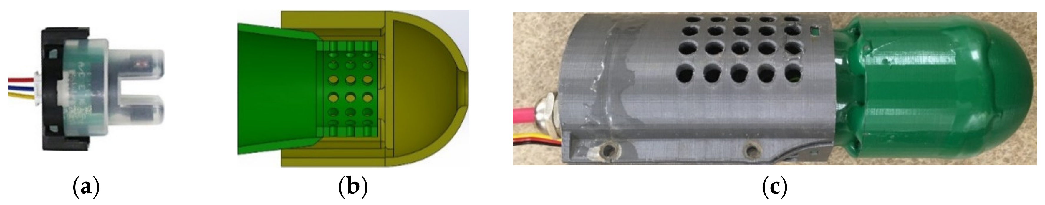
Figure 1.
(a) Turbidity sensor, (b) cut-away view of the case design, and (c) 3D printed final assembly of the probe case for dissolved oxygen (DO), pH, electrical conductivity (EC), temperature, and turbidity probes.
Figure 1.
(a) Turbidity sensor, (b) cut-away view of the case design, and (c) 3D printed final assembly of the probe case for dissolved oxygen (DO), pH, electrical conductivity (EC), temperature, and turbidity probes.

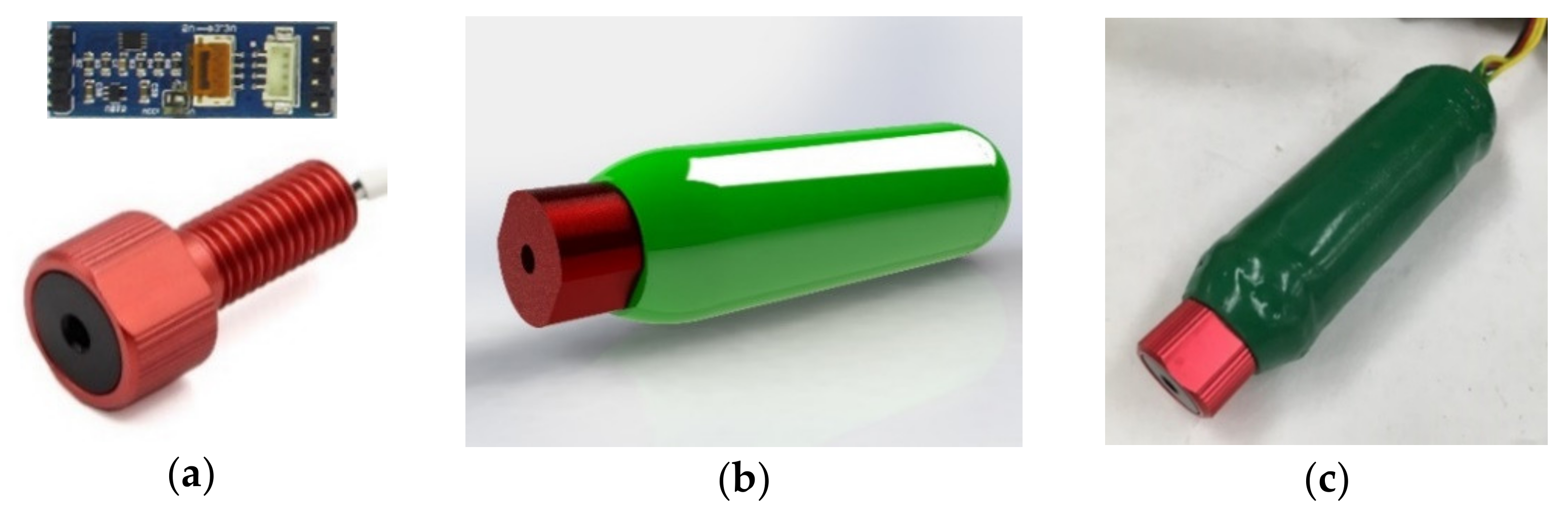
Figure 2.
The pressure sensor components; (a) pressure sensor and voltage converter, (b) perspective view of waterproof case in SolidWorks, and (c) 3D printed and sealed pressure sensor.
Figure 2.
The pressure sensor components; (a) pressure sensor and voltage converter, (b) perspective view of waterproof case in SolidWorks, and (c) 3D printed and sealed pressure sensor.

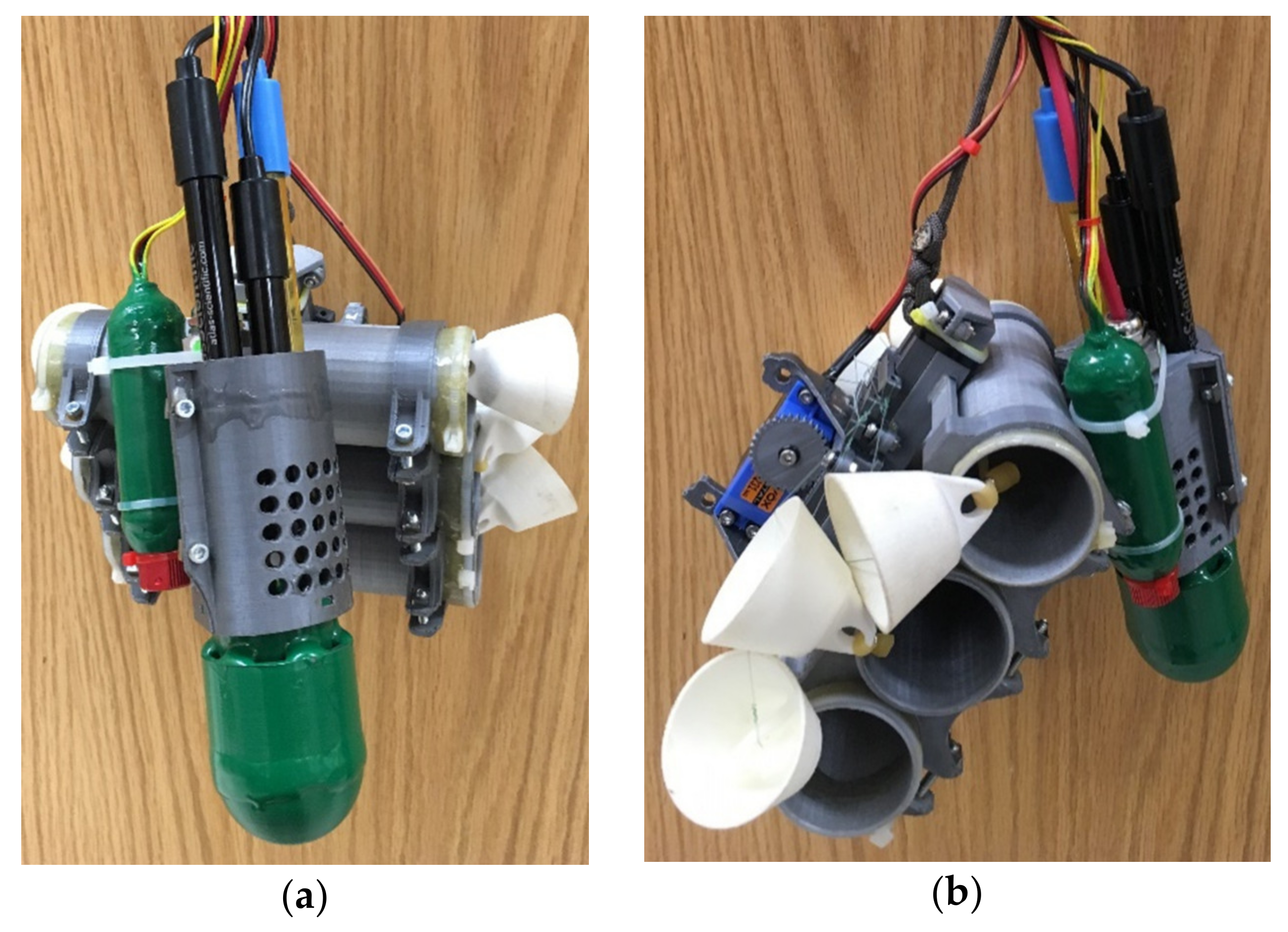
Figure 3.
Water Sampling Device (WSD) and its components; (a) front view with pressure sensor, turbidity sensor, and probes, (b) side view with open cartridges and servo mechanism.
Figure 3.
Water Sampling Device (WSD) and its components; (a) front view with pressure sensor, turbidity sensor, and probes, (b) side view with open cartridges and servo mechanism.

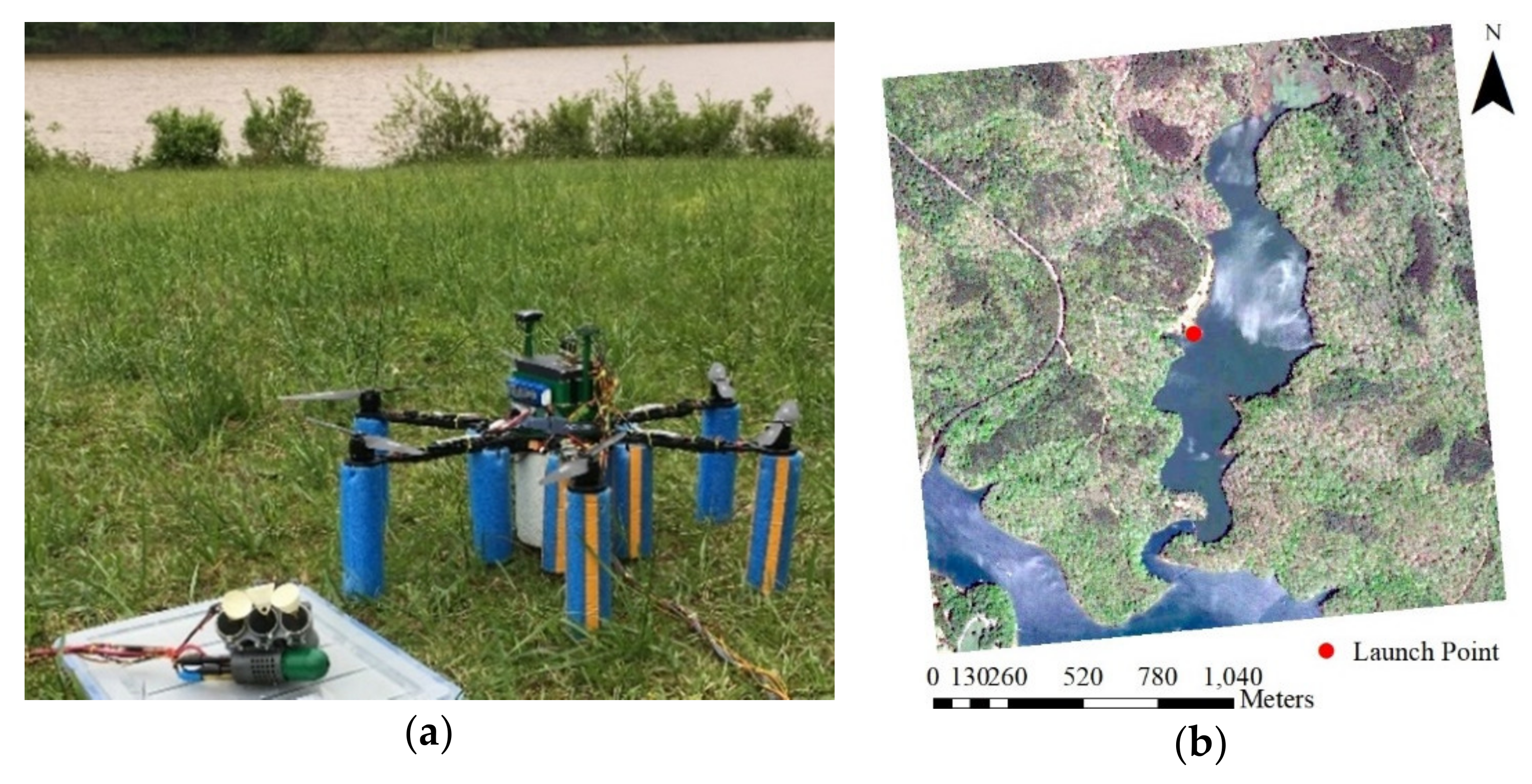
Figure 4.
(a) Unmanned Aerial Vehicle (UAV) integrated WSD and (b) the launch location in Lake Issaqueena.
Figure 4.
(a) Unmanned Aerial Vehicle (UAV) integrated WSD and (b) the launch location in Lake Issaqueena.

Figure 5.
Experiment site and water sampling points with mission plan boundary at the lake Issaqueena.
Figure 5.
Experiment site and water sampling points with mission plan boundary at the lake Issaqueena.

Figure 6.
UAV flight pattern of adaptive water sampling method.

Figure 7.
The WSD self-activation flow chart.

Figure 8.
Correlation of depth measurements and actual sensor depth in the test tube.

Figure 9.
Comparison of turbidity measurements obtained from turbidity sensor and turbidity standard solutions.
Figure 9.
Comparison of turbidity measurements obtained from turbidity sensor and turbidity standard solutions.

Figure 10.
Sensor node equilibrium times for each probe.

Figure 11.
Comparison of the turbidity measurements of sampling locations in Lake Issaquena with the sensor node and the turbidimeter.
Figure 11.
Comparison of the turbidity measurements of sampling locations in Lake Issaquena with the sensor node and the turbidimeter.

Figure 12.
Water quality maps that were created from adaptive water sampling experiment data.


Table 1.
WSD self-activation results based on standard solutions.
| Parameter | Lower Limit | Higher Limit | Successful Self Activation | Failed Self Activation | Success Rate (%) |
|---|---|---|---|---|---|
| DO | 6 mg/L | 12 mg/L | 21 | 1 | 96 |
| pH | 6.5 | 9.5 | 20 | 2 | 91 |
| EC | 100 µS/cm | 2000 µS/cm | 21 | 1 | 96 |
| Temperature | 20 °C | 35 °C | 22 | 0 | 100 |
| Total | N/A | N/A | 84 | 4 | 96 |
Table 2.
In situ water quality measurements with the WSD and self-activation status by sampling locations.
Table 2.
In situ water quality measurements with the WSD and self-activation status by sampling locations.
| Sample Location | In Situ Measurements with WSD | Parameters Outside the Allowable Limits | Self-Activation of Cartridges | |||
|---|---|---|---|---|---|---|
| DO (mg/L) | pH | EC (µS/cm) | Temp (°C) | |||
| 1 | 8.18 | 5.08 | 7.52 | 18.21 | pH, EC, Temperature | Successful |
| 2 | 8.39 | 4.98 | 6.51 | 18.81 | pH, EC, Temperature | Successful |
| 3 | 8.55 | 5.59 | 6.96 | 18.49 | pH, EC, Temperature | Successful |
| 4 | 8.57 | 5.15 | 6.8 | 16.06 | pH, EC, Temperature | Successful |
| 5 | 8.27 | 5.37 | 6.49 | 18.26 | pH, EC, Temperature | Successful |
| 6 | 8.68 | 5.92 | 6.82 | 16.08 | pH, EC, Temperature | Successful |
| 7 | 8.64 | 5.28 | 6.77 | 17.31 | pH, EC, Temperature | Successful |
| Avg. | 8.47 | 5.34 | 7 | 18 | N/A | N/A |
© 2020 by the authors. Licensee MDPI, Basel, Switzerland. This article is an open access article distributed under the terms and conditions of the Creative Commons Attribution (CC BY) license (http://creativecommons.org/licenses/by/4.0/).
Share and Cite
MDPI and ACS Style
Koparan, C.; Koc, A.B.; Privette, C.V.; Sawyer, C.B. Adaptive Water Sampling Device for Aerial Robots. Drones 2020, 4, 5. https://0-doi-org.brum.beds.ac.uk/10.3390/drones4010005
AMA Style
Koparan C, Koc AB, Privette CV, Sawyer CB. Adaptive Water Sampling Device for Aerial Robots. Drones. 2020; 4(1):5. https://0-doi-org.brum.beds.ac.uk/10.3390/drones4010005
Chicago/Turabian StyleKoparan, Cengiz, A. Bulent Koc, Charles V. Privette, and Calvin B. Sawyer. 2020. "Adaptive Water Sampling Device for Aerial Robots" Drones 4, no. 1: 5. https://0-doi-org.brum.beds.ac.uk/10.3390/drones4010005