Article

High Resolution Geospatial Evapotranspiration Mapping of Irrigated Field Crops Using Multispectral and Thermal Infrared Imagery with METRIC Energy Balance Model

1
Center for Precision and Automated Agricultural Systems, Irrigated Agriculture Research and Extension Center, Washington State University, Prosser, WA 99350, USA
2
Department of Biological Systems Engineering, Washington State University, Pullman, WA 99164, USA
*
Authors to whom correspondence should be addressed.
Submission received: 29 July 2020 / Revised: 24 August 2020 / Accepted: 28 August 2020 / Published: 1 September 2020
(This article belongs to the Special Issue Feature Papers of Drones)

Abstract

:
Geospatial crop water use mapping is critical for field-scale site-specific irrigation management. Landsat 7/8 satellite imagery with a widely adopted METRIC (Mapping Evapotranspiration at high Resolution with Internalized Calibration) energy balance model (LM approach) estimates accurate evapotranspiration (ET) but limits field-scale spatiotemporal (30 m pixel−1, ~16 days) mapping. A study was therefore conducted to map actual ET of commercially grown irrigated-field crops (spearmint, potato, and alfalfa) at very high-resolution (7 cm pixel−1). Six small unmanned aerial system (UAS)-based multispectral and thermal infrared imagery campaigns were conducted (two for each crop) at the same time as the Landsat 7/8 overpass. Three variants of METRIC model were used to process the UAS imagery; UAS-METRIC-1, -2, and -3 (UASM-1, -2, and -3) and outputs were compared with the standard LM approach. ET root mean square differences (RMSD) between LM-UASM-1, LM-UASM-2, and LM-UASM-3 were in the ranges of 0.2–2.9, 0.5–0.9, and 0.5–2.7 mm day−1, respectively. Internal calibrations and sensible heat fluxes majorly resulted in such differences. UASM-2 had the highest similarity with the LM approach (RMSD: 0.5–0.9, ETdep,abs (daily ET departures): 2–14%, r (Pearson correlation coefficient) = 0.91). Strong ET correlations between UASM and LM approaches (0.7–0.8, 0.7–0.8, and 0.8–0.9 for spearmint, potato, and alfalfa crops) suggest equal suitability of UASM approaches as LM to map ET for a range of similar crops. UASM approaches (Coefficient of variation, CV: 6.7–24.3%) however outperformed the LM approach (CV: 2.1–11.2%) in mapping spatial ET variations due to large number of pixels. On-demand UAS imagery may thus help in deriving high resolution site-specific ET maps, for growers to aid in timely crop water management.

1. Introduction

Satellite-based remote sensing (RS) has been extensively used with energy balance models for regional scale evapotranspiration (ET) mapping [1,2,3,4,5,6,7,8]. One such widely adopted model is Mapping ET at high-resolution with Internalized Calibration (METRIC) [9,10]. The METRIC model uses Landsat 5/7/8, or Terra and Aqua satellite based multispectral and thermal infrared imagery data to compute ET as an energy balance residue. METRIC is advantageous for its independence from surface conditions, stabilized sensible heat flux (H) estimations, and internal calibration using hot and cold anchor pixels. This internal calibration compensates for any computational biases that arise from atmospheric dynamics, surface albedo, net radiation (Rn), surface temperature (Ts), air temperature (Ta), soil heat flux (G), and wind speed (u). The METRIC model has been evaluated for a wide range of irrigated field and orchard/tree crops under different agroclimatic zones, with studies reporting ET estimation errors in the ranges of 1 to 11% [11,12,13,14,15,16,17,18,19,20,21,22].
Conventional METRIC uses high orbiting satellite imagery and as a result has low spatial (~30 m pixel−1 for Landsat and 1 km pixel−1 for Terra and Aqua satellites) and temporal resolution (~16 days for Landsat) ET maps. Cloud cover is an additional challenge. Alternatively, the ET mapping can be improved spatiotemporally using unmanned aerial system (UAS)-based imagery data [23,24,25] that can be collected on-demand [7,26,27,28,29]. Recent UAS technology advancements have enabled rapid assessment of crop vigor and soil characteristics, crop water requirements, disease infestation, and yield prediction [23,26,27,28,29,30]. Pertinent to ET estimation, Chavez et al. [27] have used airborne imagery data with METRIC and reported daily ET errors of 9% for corn and sorghum grown on experimental plots. Similarly, Ortega-Farias et al. [31] have estimated ET using UAS imagery for a drip irrigated olive orchard and reported maximum errors below 7%. Brenner et al. [32] have estimated latent heat fluxes (LE) from energy balance model for irrigated grassland and observed errors below 10%. They also reported strong correlations of up to 0.9 between estimated LE and that measured with eddy covariance system. Furthermore, Paul et al. [33] have reported suitability of UAS based imagery in conjunction with METRIC model to estimate ET with maximum errors below 11% for irrigated forage, corn, and sorghum crops. All these studies have experimentally illustrated potential of UAS based RS data for accurate ET estimation. However, ET mapping of commercial crop fields from the grower’s perspective has been limited for site-specific irrigation management. Additionally, the differences in spatial ET mapping due to in-field elevation variability and near-site available meteorological inputs have not been evaluated with respect to the conventional satellite-based METRIC approach.
Agricultural growers typically use standard crop coefficients or point soil moisture measurements for irrigation scheduling and supply water at a constant rate to the entire field. This results in either under or over irrigation. Satellite imagery also restricts site-specific irrigation management due to low spatiotemporal resolutions. Alternatively, ET mapping with UAS imagery could be directly applicable to growers. This study therefore assesses the suitability of UAS-based imagery to geospatially map actual ET at very high-resolution relative to the satellite-based imagery. The spatial ET differences resulting due to local field conditions and near-site meteorological inputs are also assessed. The specific objectives are: (1) ET mapping of irrigated spearmint, potato, and alfalfa crops under commercial operations using UAS-based multispectral and thermal infrared imagery with variants of METRIC energy balance model, and (2) parametric comparison of the model outputs and spatial ET variation assessment potentials from UAS imagery with that from satellite (Landsat 7/8) imagery.

2. Materials and Methods
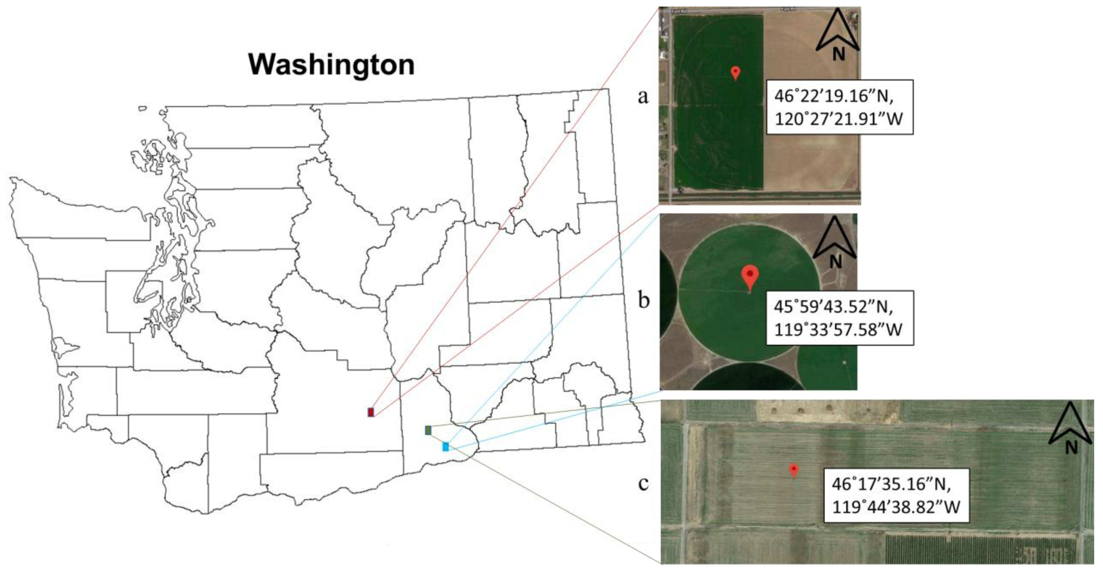
2.1. Field Sites

Selected were commercial sites (Table 1) planted with spearmint (Cultivar (cv.) Native) in Toppenish, potato (cv. Russet Burbank) in Paterson, and alfalfa (cv. FD-4) in Prosser in Washington state (Figure 1). All sites received limited rainfall (<60 mm), and seasonal mean air temperatures up to 20 °C and cumulative reference ET between 1000 to 1200 mm were observed.

2.2. Data Acquisition Campaigns

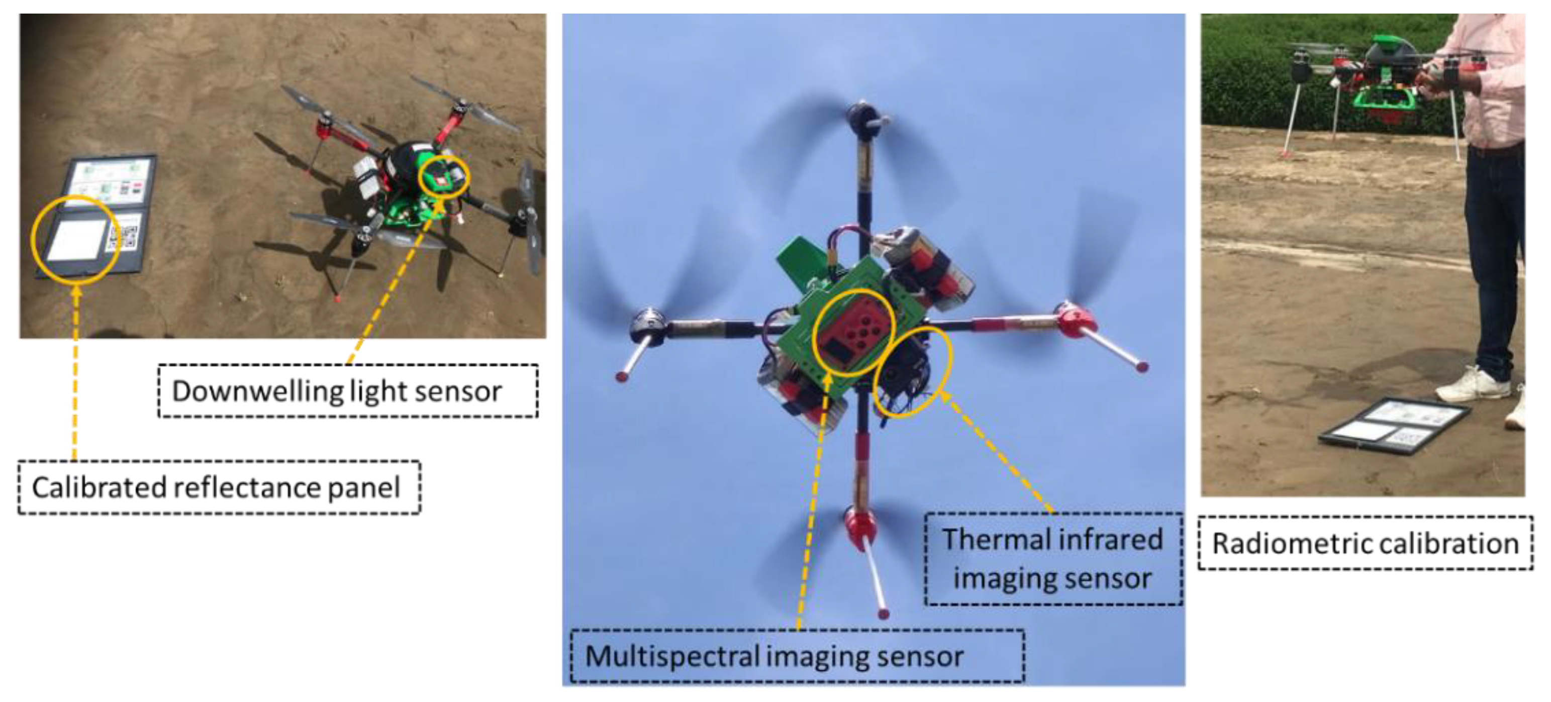
2.2.1. UAS-Based Imagery

A UAS (ATI AgBOT™, Aerial Technology International, Wilsonville, OR, USA) was deployed for imagery data acquisition (Figure 2). On-board was a multispectral imaging sensor (RedEdge 3, MicaSense, Inc., Seattle, WA, USA) with Blue (B, 475 ± 10 nm), Green (G, 560 ± 10 nm), Red (R, 668 ± 5 nm), Red Edge (RE, 717 ± 5 nm), and Near Infrared (NIR, 840 ± 20 nm) wavebands and a radiometric calibrated thermal infrared imaging sensor (11,000 ± 3000 nm, Tau 2 640, FLIR Systems, Wilsonville, OR, USA). Image-specific geotags for the multispectral sensor were received from the global positioning system (GPS) receiver on-board UAS and that for thermal sensor were received from an independent GPS receiver (ThermalCapture GPS, TeAx Technology GmbH, Wilnsdorf, Germany). On-board the UAS was also a downwelling light sensor (DLS, MicaSense, Inc., Wilnsdorf, WA, USA) facing skyward to embed the solar irradiance data in the imagery spectrum during flights.
UAS flights were configured using a ground control software (MissionPlanner, version 1.3.49, Ardupilot, USA) for altitude of 100 m above ground level (AGL) to acquire multispectral and thermal images at ground sampling resolutions of 7 and 13 cm pixel−1, respectively. The software aided in configuring the multispectral sensor to acquire images at 85% front and 75% side overlaps. The thermal imaging sensor was configured independently to acquire frames at 3 Hz to ensure image overlaps of 90–95%. Imagery data was stored on-board in respective memory cards for the two sensors. A calibrated reflectance panel (CRP, Micasense Inc., Seattle, WA, USA) was imaged before and after each flight and these reference images were used for radiometric calibration of the multispectral imagery (Figure 2).
Total six UAS flights were conducted in summers of 2018 (two missions/site × 3 sites) during the dates and approximate times of the Landsat 7/8 overpass. UAS imagery for spearmint crop was collected 10 days before the first harvest (dataset-1) and 37 days before the second harvest (dataset-2). Imagery for the potato crop was acquired 72 days (dataset-3) and 48 days before harvest (DBH, dataset-4). Data for the alfalfa crop was collected 2 days before the first harvest (dataset-5) and 7 days before the second harvest (dataset-6).

2.2.2. Satellite-Based Imagery and Weather Data

Landsat 7/8 imagery datasets and 1-arc SRTM (Shuttle Radar Topography Mission) digital elevation models (DEM) were downloaded for the data collection days (Table 2). Weather data logged at every 15 min was downloaded from the nearest (1–5 km) stations (AgWeatherNet, Washington State University, Washington, WA, USA). All the data collected on a day were grouped to have a total of six datasets (see Table 2) ready for analysis.

2.3. Imagery Analysis and METRIC Models Implementation

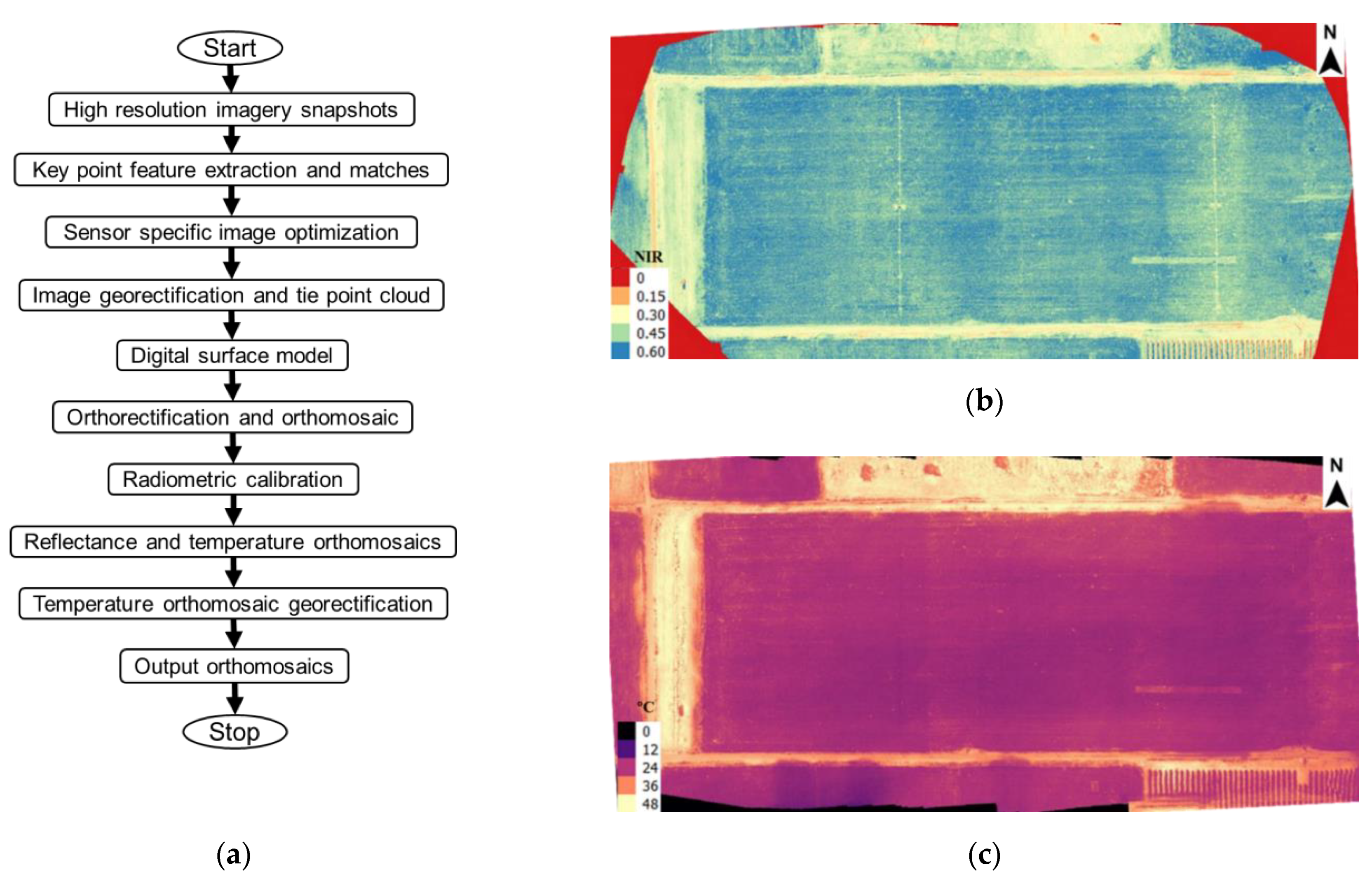
2.3.1. Preprocessing

UAS imagery was initially processed to obtain orthomosaics of the study site(s) through a series of image stitching operations (Figure 3a) in a photogrammetry and mapping software (Pix4D Mapper, Pix4D, Inc., Lausanne, Switzerland). Independent surface temperature orthomosaic was then georeferenced and resampled to the multispectral orthomosaic (7 cm pixel−1) in Quantum Geographic Information System (QGIS) platform (ver.2.18.16, Open Source). The “Georeferencer” tool with “Thin Plate Spline” as the transformation type was used for georeferencing and the “Nearest Neighborhood” method was used for resampling. Five surfaces reflectance (B, G, R, RE, and NIR (Figure 3b)), one surface temperature (Figure 3c) and a DEM orthomosaic were obtained for each UAS mission.

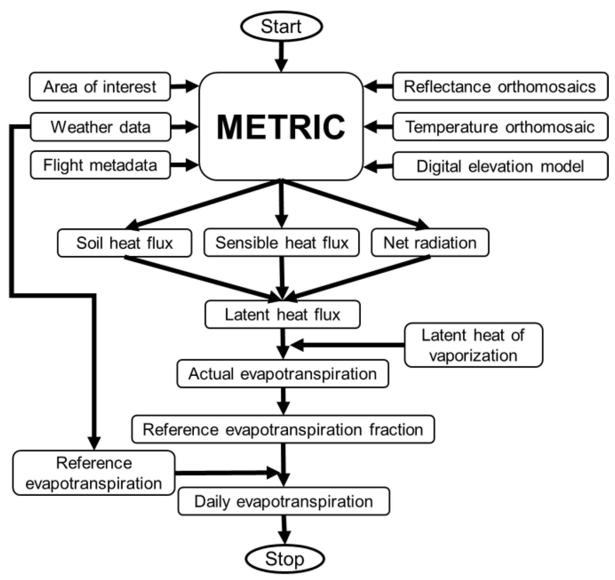
2.3.2. METRIC Model Implementation

The METRIC model is detailed in Allen et al. [9]. Briefly, model computes Rn, G, H and residual LE within the blending height (100–200 m AGL) which can be converted to actual water loss to the atmosphere (ET). METRIC eliminates the need for accurate surface temperature (Ts) measurements. It uses ground weather station-based reference ET (ETr, alfalfa crop based) for internal calibration and reduction of biases related to satellite imagery. The internal calibration indexes near-surface temperature gradients to the radiometric Ts using extreme hot and cold anchor pixels. The model was primarily developed for agricultural fields and does not need crop specific inputs. This enhances METRIC’s applicability to high-resolution RS data. Small UAS based RS data captures distinct features of soil, vegetation, or mixed regions that can improve internal calibration of METRIC model with respect to the study environment [26,27,28,29,33].
Conventional METRIC maps regional ET for 185×185 km scene size and all its assumptions might not necessarily apply at the field-scale. Therefore, METRIC model was implemented with three variant approaches. The resulting approaches are named as UAS-METRIC-1, -2, and -3 (UASM-1, -2, and -3) with pertinent modification highlights summarized in Table 3. UASM-1 (Figure 4) was implemented to observe relative differences only due to UAS imagery specific inputs that include (i) scene metadata from flight missions, (ii) surface albedo from on-board multispectral imager, and (iii) high-resolution DEM. All other equations were identical as the conventional METRIC. Similar to LM, leaf area index (LAI) in UASM-1 was calculated using soil adjusted vegetation index (SAVI) with background adjustment factor (L) of 0.1 for high crop cover [34,35]. UASM-2 was employed for two reasons: (i) possibility to reduce model input data needs from the grower perspective and (ii) to assess pertinent differences caused by the DEM typical to flat agricultural fields located in non-terrain regions. Implementation of UASM-2 was identical to UASM-1 except that UASM-2 used a flat DEM for local field conditions. This scenario forced surface slopes and aspects to zero and elevation as the mean of all pixels in the DEM.
UASM-3 considered site-specific energy balance inputs typical to agricultural field plots imaged in this study. Pertinent modifications include (i) DEM as per field conditions (as in UASM-2), (ii) LAI calculation from spatial fraction canopy cover (FCC), (iii) incoming shortwave radiation (ISWR) from the nearest open field weather station, (iv) incoming longwave radiation (ILWR) calculation using air temperature (Ta), and (v) momentum roughness length (MRL) calculated without surface slope (S) adjustments. The LAI calculation in UASM-3 were based on the fact that surface features (i.e., soil, vegetation, and mixed) could be distinctively captured in every pixel [28,29,30] of high-resolution imagery. FCC was first derived from the normalized difference vegetation index (NDVI) [28,36,37] and soil was segmented using NDVI vegetation threshold mask (>0.3) to ensure LAI for the vegetation only. ISWR measurements from the nearest weather station may be assumed as actual shortwave radiation on the surface for the fact that these are open-field stations installed at 2 m AGL and located within 5 km radius from the study sites. Moreover, conventional ISWR calculation might get affected by cloud cover and other atmospheric dynamics [38,39]. Ta from nearest weather station was used to calculate ILWR and can be assumed constant for a field (Stefan Boltzmann’s law, [40]).
For comparisons, Landsat imagery was processed through the conventional METRIC model as described in a “R package” (water, [41,42]), hereafter abbreviated as LM (Landsat-METRIC) approach. Level-2 surface reflectance products were downloaded for Landsat 8 while such products were calculated within the package for Landsat 7 datasets. Similar to the LM approach, all UASM approaches performed an energy balance within the blending height and used the conventional automated approach of selecting anchor pixels.

2.4. Output Comparisons

This study aimed at evaluating spatial ET maps from UAS based remote sensing (RS) data relative to satellite-based RS data for crops grown in commercial farming operations. As the conventional METRIC model is well-established for spatial ET mapping for its corroboration in over 25 countries and in almost all types of agroclimatic zones [22], the additional field validation was deemed not necessary, i.e., outside the scope of the study. Thus, we did not conduct ground-reference ET measurements.
Since the energy balance computations with LM approach were performed for images of 180 km × 180 km dimension, intermediate and final output maps were clipped to the study site areas covered by the UAS flights. The mean, standard deviation (SD), and coefficients of variation (CV, %) to assess spatial variability capturing potentials of ET pixels from LM (ETLM) and UASM-1, -2, and -3 approaches (ETUASM) were calculated. Percentage absolute departures of mean ET (ETdep,abs, Equation (1)) from all UAS-based approaches with respect to that from the LM approach were also calculated. Next, ET maps from all UAS-based approaches were resampled to the resolution equal to ET maps from LM approach (30 m pixel−1) using the “Nearest Neighborhood” method and region of interest (ROI) samples were randomly extracted. Sample ET from these ROIs were compared using root mean square difference (RMSD) and Pearson’s linear correlation (r) at 5% significance (RStudio, Inc., Boston, MA, USA).
ETdep,abs (%) = (|ETUASMETLM| × 100)/ETLM

3. Results

Major energy balance computations from the UASM and LM approaches are presented in the following subsections. Results pertinent to spearmint (Table 4, Figure 5a–d and Figure 6), potato (Table 5, Figure 5e–h and Figure 7), and alfalfa crops (Table 6, Figure 5i–l and Figure 8) are also presented.

3.1. Crop Vigor

The UAS imagery mapped crop vigor indicators of SAVI (Mean: 0.7–0.9, SD: 0.1–0.2) and NDVI (Mean: 0.8–0.9, SD: 0.1–0.2) similar to the Landsat imagery mapped SAVI (Mean: 0.7–0.85, SD: ~0.02) and NDVI (Mean: 0.8–0.9, SD: 0.02–0.1). The mean LAI from LM approach ranged between 4–6 m2 m−2 and that from UASM-1/-2 and -3 ranged from 5.1–5.8 m2 m−2 and 3.5–5.9 m2 m−2, respectively. Mean FCC ranges were 0.91–0.93 (SD: ~0.14) for spearmint, 0.92–0.93 (SD: ~0.1) for potato, and 0.8–0.9 (SD: 0.1–0.24) for the alfalfa fields. All these estimates show high density vegetation also observed at the sites.

3.2. Net Radiation, Soil Heat and Sensible Heat Fluxes

The mean ISWR ranges from the LM, UASM-1, -2, and -3 approaches were 819–903, 817–927, 818–921, and 737–949 W m−2, respectively. Mean ILWR ranges from those approaches were 337–396, 296–347, 296–347, and 321–375 W m−2, respectively. Mean outgoing longwave radiation (OLWR) from the LM, UASM-1, -2, and -3 approaches ranged between 440–514, 381–451, 381–451, and 381–451 W m−2, respectively and Rn ranges were 508–594, 596–685, 596–685, and 564–716 W m−2. Mapped G from the LM, UASM-1, -2, and -3 approaches were in the ranges of 23.8–63.6, 19.4–35.9, 19.4–35.9, and 18.2–36.1 W m−2, respectively and mean H ranges were 60–181, 114–237, 126–250, and 127–233 W m−2, respectively.

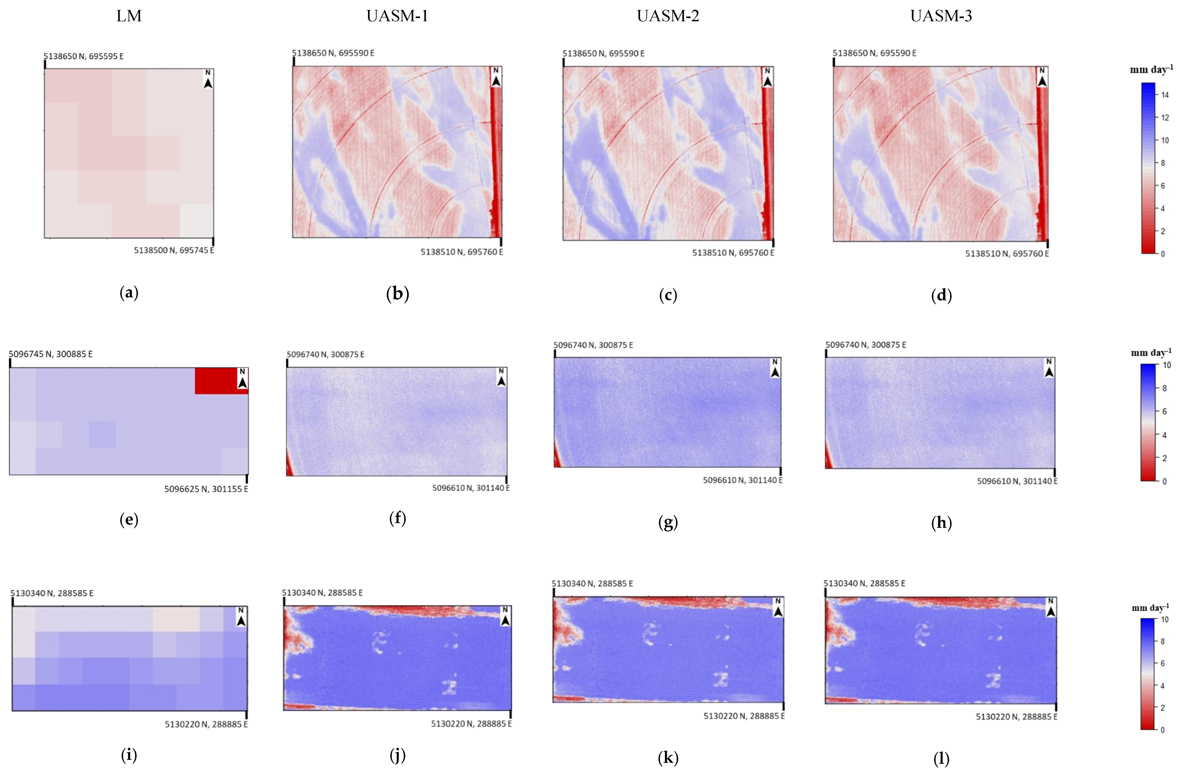
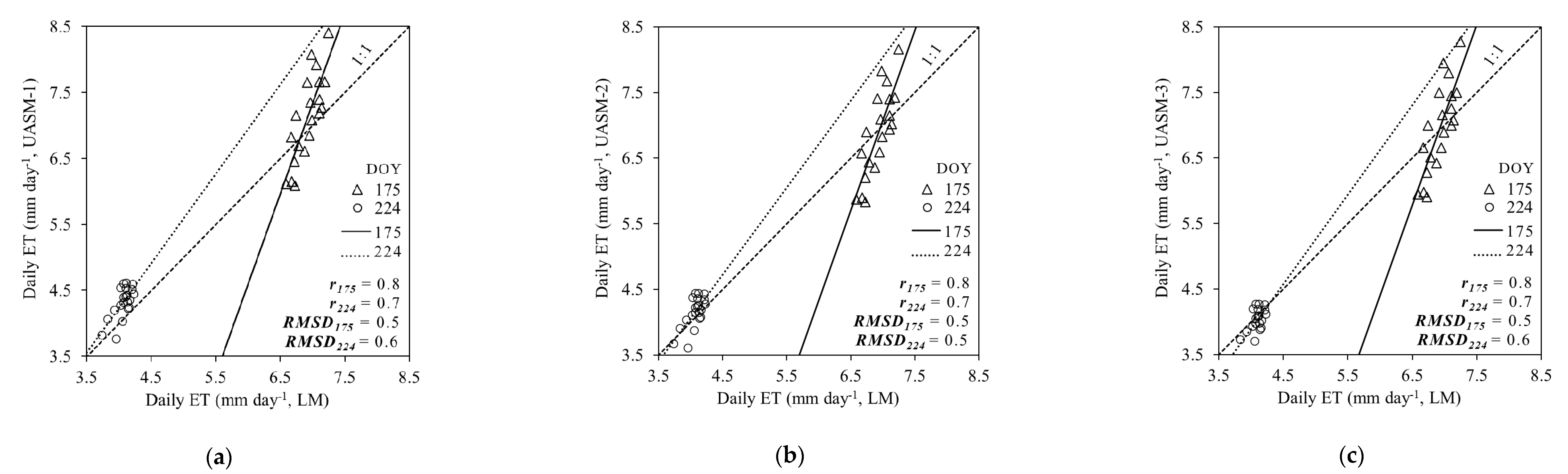
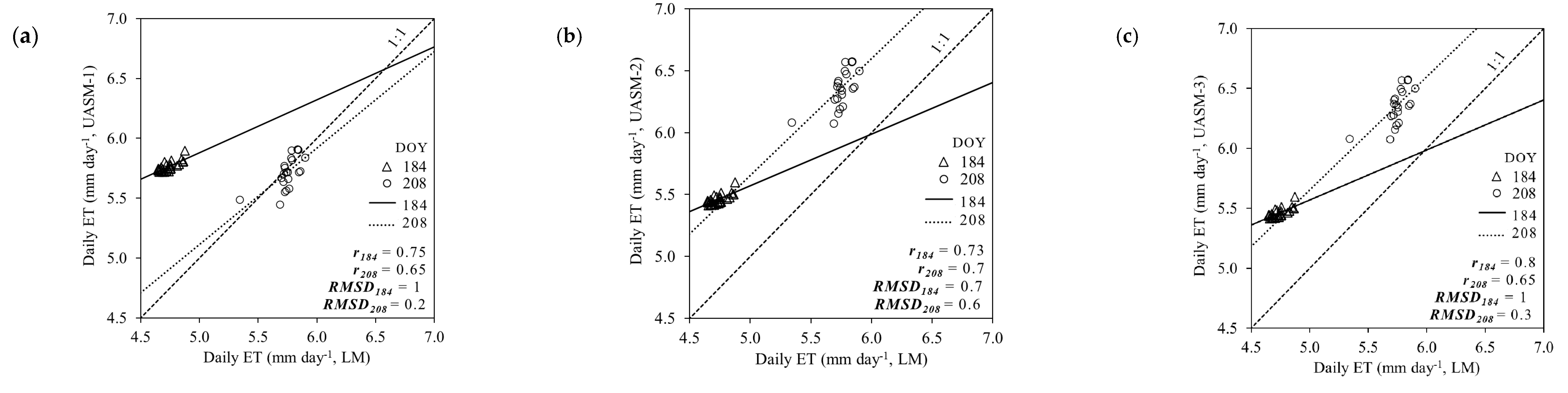
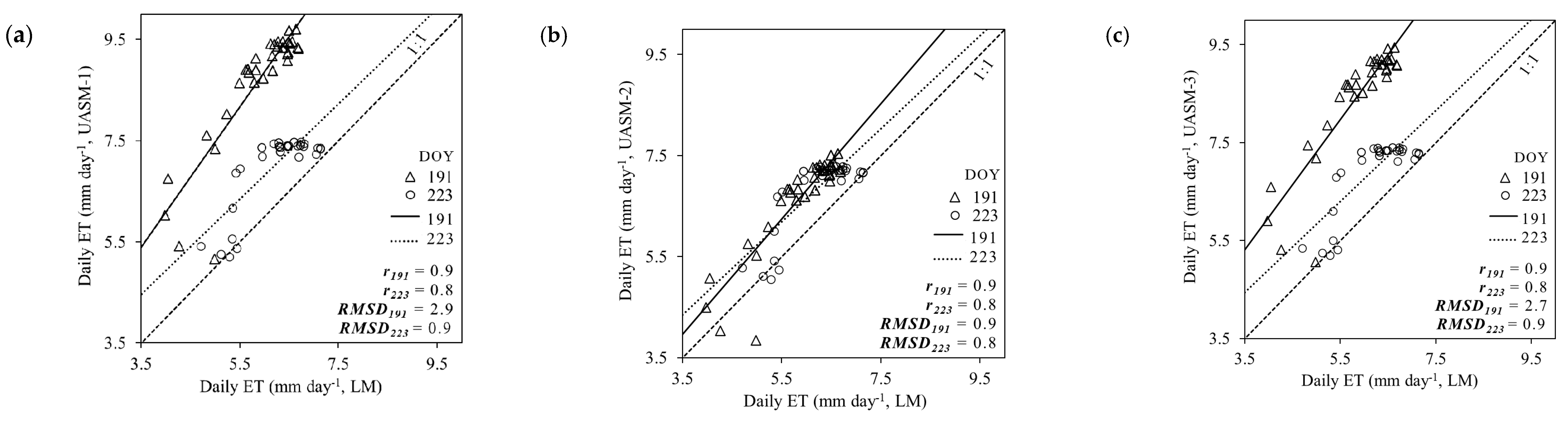
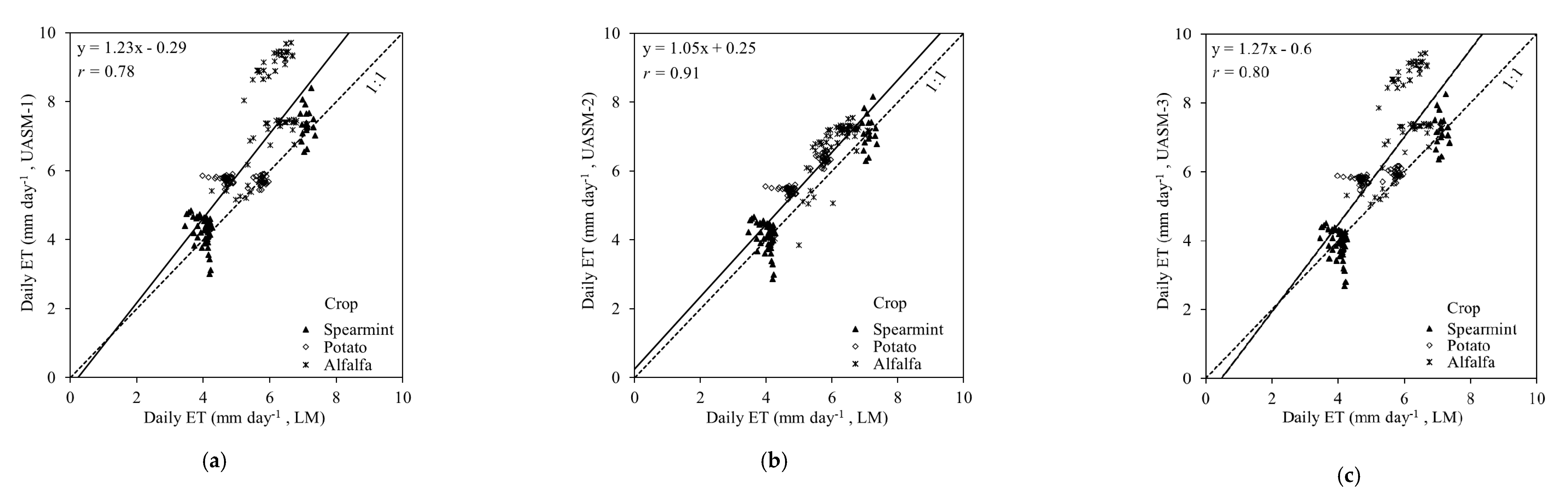
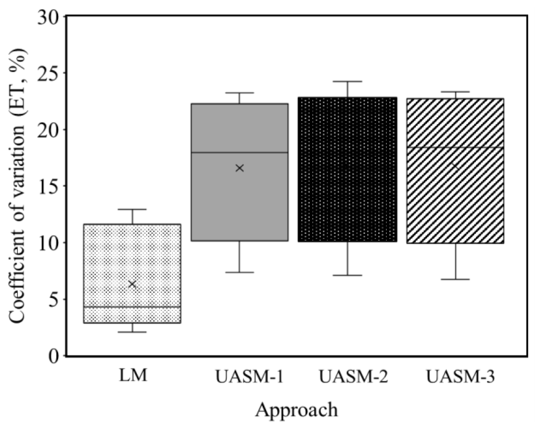
3.3. Daily Evapotranspiration

The mean ranges of mapped instantaneous ET (ETinst) from the LM, UASM-1, -2, and -3 approaches were 0.5–0.7, 0.5–0.7, 0.5–0.7, and 0.5–0.7 mm h−1, respectively and pertinent ETrF ranges were 0.7–0.9, 0.74–0.95, 0.7–1, and 0.7–0.93, respectively. ETr24 for the six datasets were 9.4, 5.2, 6.3, 6.5, 8.8, and 8.5 mm day−1. The mean of mapped daily ET from LM, UASM-1, -2, and -3 approaches were in the ranges of 4–7, 4.3–8.4, 4.1–6.7, and 3.9–8.2 mm day−1, respectively. Ranges of absolute departures of daily ET (ETdep,abs) from UASM-1, -2, and -3 were 0.4–20.8, 2.0–14.4, and 2.2–21% of ETLM, respectively for the selected crops. Highest correlations and minimum RMSDs (Figure 6, Figure 7, Figure 8 and Figure 9) were observed for UASM-2 (r: 0.66–0.9, RMSD: 0.5–0.9) followed by UASM-1 (r: 0.65–0.9, RMSD: 0.2–2.9) and UASM-3 (r: 0.65–0.9, RMSD: 0.5–2.7) approaches compared to the LM approach.

4. Discussion

4.1. Crop Vigor

High spatial variability in crop vigor was captured by the UAS imagery. Soil background adjustment factor (L) of 0.1 as in the LM calculated similar SAVI with the UAS imagery for selected crops [34,35]. Higher NDVI compared to SAVI for some datasets may be due to the saturation effects ignored in SAVI [43]. Soil-segmented FCC mapped similar LAI from UASM-3 as from the LM approach. MRL estimates from UAS and Landsat imagery were also similar. Slight differences in MRL from UASM-1 and -2 approaches were mainly due to surface slope factor in the case of UASM-1 approach and that between UASM-1 and -3 approaches were due to LAI and DEM inputs.

4.2. Net Radiation and Soil Heat Flux

The ISWR from LM, UASM-1, and -2 approaches were similar and slight differences were due to the DEM inputs. ISWR from UASM-3 approach was different due to its direct measurement source (nearest weather station). Such ISWR measurements may be assumed actual compared to the standard computations for the weather stations installed near study sites (within 5 km) approximately at 2 m height [38,39]. Higher ILWR estimates from the LM approach compared to UASM-1 and -2, were primarily due to higher Ts. Minor ILWR differences between LM and UASM-1 or -2 approaches would be due to slightly different DEMs used to calculate atmospheric transmissivities. ILWR computation in UASM-3 approach used Ta as the input (Stefan Boltzmann’s law) instead of the Ts [40] and no variation for use of a single value may be assumed realistic at field level. OLWR differences between LM and UASM approaches were primarily due to differences in Ts from pertinent imaging systems. Similar OLWR from UASM-1, -2, and -3 approaches showed no effect of LAI differences that contribute only 1% to the surface emissivity calculations. Rn and G estimate differences between UASM and LM approaches can be attributed to differences between ISWR, ILWR, OLWR and surface albedo computations. While no Rn and G differences between UASM-1 and UASM-2 approaches were due to negligible differences between ISWR, ILWR, and OLWR. Such differences between UASM-1 and UASM-3 approaches were due to the ISWR and ILWR differences. Since high LAI was observed in all imaging campaigns, slightly high variations in OLWR and Rn may be expected during initial days of plantation (Low LAI).

4.3. Sensible Heat Flux

Differences between H estimates from LM and UASM approaches were primarily due to Ts differences, and secondarily due to different internal calibrations. As the Landsat 7/8 imagery has coarse resolution (~30 m pixel−1), it might not be readily possible to find uniform hot and cold anchor pixels. This demands for additional flexibility in anchor pixel identification also suggested by Jaafar et al. [42]. Contrarily, it was easier with the UAS-based approaches (~7 m pixel−1) to identify anchor pixels within the imaged field area (Table 7). Irrigated crops would have also facilitated identification of highly transpiring cold anchor pixels alike the reference alfalfa. H differences between UASM-1, -2, and -3 could be due to LAIs, MRLs, Rn, and G differences in the different cold pixels that resulted in different internal calibrations.

4.4. Daily Evapotranspiration

Similar ET was mapped from all UASM approaches compared to the LM approach (Figure 5, Figure 6, Figure 7, Figure 8 and Figure 9). However, UASM approaches showed larger potential for assessing spatial variations in field ET maps (Figure 10) due to large number of pixels [21]. The ET differences between LM, UASM-1, and -3 approaches were large for dataset-5 (alfalfa field) and dataset-3 (potato field) primarily due to the internal calibration differences, H and Rn differences. The ETrF for alfalfa crop in dataset-6 was high compared to dataset-5 showing more matured crop at 2 DBH than 7 DBH. Notable ETrF differences between LM and UASM approaches could also be due to accumulated differences between the intermediate outputs. ETrFs for selected crops did not exceed 1.1, complying to the cold anchor pixel assumption (1.05 × ETr, [9]). UASM-3 approach (METRIC model modified to local conditions) can also provide reliable geospatial ET maps as LM. As also reported by Paul et al. [33], G and H differences between LM and UAS approaches did not influence daily ET maps for irrigated field crops due to small magnitudes. UASM approaches indicate their versatility for geospatial ET mapping for a range of similar crops as spearmint, potato and alfalfa (r: 0.8–0.9). However, additional parametrization may be needed for different crop physiologies [21,27]. An average 10% uncertainty of UASM approaches for point scale ET might be acceptable as discussed in prior research studies that used similar UAS imagery with METRIC model [29,33]. Flight missions within solar noon ± 2 h could have produced comparable and reasonable ETrF used for 24-h [44].

5. Conclusions

Agricultural growers are highly dependent on generalized crop coefficients or point measurements (soil moisture, sap flow, etc.) for irrigation scheduling and are restrictive towards satellite-based remote sensing approaches due to low spatiotemporal resolution and cloud cover issues. Considering the critical need for geospatial ET mapping towards precision irrigation management, ET of irrigated field crops was mapped using very high resolution multispectral and thermal infrared imagery. Three variants of standard METRIC energy balance model modified as per UAS and local conditions were used to process UAS imagery and their performance was evaluated relative to standard LM approach.
Increased spatial resolution did not influence the mean field-scale ET (low RMSD: 0.2–1.0 mm day−1, ETdep,abs: 0.4–21.2%, and r: 0.7–0.9). However, high spatial ET variation potential was assessed in UAS derived maps (6.7–24.3%) compared to the Landsat satellite derived maps (2.1–11.2%). Variants of UASM models performed very similar to the LM approach for irrigated field crops; spearmint (ETdep,abs: 0.4–6.2% and r: 0.7–0.8), potato (ETdep,abs: 0.9–21.2% and r: 0.7–0.8), and alfalfa (ETdep,abs: 7.2–9.9% and r: 0.8–0.9). UASM-2 showed highest similarity with the LM approach (RMSD: 0.5–0.9 mm day−1 and r: 0.7–0.9) for very similar energy balance outputs. ET differences between LM and UAS based approaches were majorly due to the internal calibrations differences that could have been affected slightly by the spatial resolution. UASM-1 could be advantageous for agricultural fields with elevation variability and resulting temperature differences due to lapse rates. UASM-1 uses high-resolution UAS imagery derived DEM inputs that can be accurately compared to the satellite based DEMs. UASM-2 could be advantageous for the crop fields where spatial variability in ground elevation is negligible, as it also reduces additional DEM data requirement for ET mapping. UASM-3 uses actual meteorological parameters of ISWR and Ta (for ILWR) measured by the automated weather station near the field site. UASM-3 could also be advantageous for ensuring LAI calculation for the areas with vegetation only, as supported by high spatial resolution to distinctly capture soil, vegetation and mixed pixels. UASM-1 and UASM-3 could also be merged for field-relevant energy balance inputs such as meteorological parameters and ground elevation variabilities to obtain more realistic crop water use maps.
ET mapping at high spatiotemporal resolution provides more control over timely monitoring of spatial crop water requirements where restrictions of cloud cover interference and imagery acquisition at 16-day interval could be avoided unlike LM approach. LM based approaches may assist in reviewal of seasonal water distribution rights while UASM approaches may assist in irrigation water savings through grower friendly and on-demand site-specific irrigation prescription maps/tools.

Author Contributions

Conceptualization, A.K.C., B.M., and L.R.K.; data curation, A.K.C. and B.M.; funding acquisition, L.R.K., R.T.P., and C.O.S.; drone flights, A.K.C. and B.M.; investigation, A.K.C. and B.M.; methodology, A.K.C., L.R.K., and C.O.S.; project administration, L.R.K., R.T.P., and C.O.S.; resources, L.R.K., R.T.P., and C.O.S.; software, A.K.C.; supervision, L.R.K., R.T.P., and C.O.S.; validation, A.K.C. and B.M.; visualization, A.K.C., B.M., L.R.K., R.T.P., and C.O.S.; writing—original draft, A.K.C.; and writing—review and editing, A.K.C., B.M., L.R.K., R.T.P., and C.O.S. All authors have read and agreed to the published version of the manuscript.

Funding

This research was funded by the USDA-National Institute of Food and Agriculture projects 1016467, WNP0745, and WNP0839, and Washington State University-CAHNRS Office of Research Emerging Research Issues Internal Competitive Grant Program.

Acknowledgments

Authors would like to thank Landon Lombers, Troy Grimes, and WSU farm management team for their assistance in providing the commercial field sites for data collection.

Conflicts of Interest

Authors declare no conflict of interest.

References

  1. Kustas, W.P.; Norman, J.M. Use of remote sensing for evapotranspiration monitoring over land surfaces. Hydrol. Sci. J. 1996, 41, 495–516. [Google Scholar] [CrossRef]
  2. Quattrochi, D.A.; Luvall, F.J.C. Thermal infrared remote sensing for analysis of landscape ecological processes: Methods and applications. Landsc. Ecol. 1999, 14, 577–598. [Google Scholar] [CrossRef]
  3. Overgaard, J.; Rosbjerg, D.; Butts, M.B. Land-surface modelling in hydrological perspective? a review. Biogeosciences 2006, 3, 229–241. [Google Scholar] [CrossRef] [Green Version]
  4. Schmidt, M.; King, E.A.; McVicar, T.R. A user-customized Web-based delivery system of hypertemporal remote sensing datasets for Australasia. Photogramm. Eng. Rem. Sens. 2006, 72, 1073–1080. [Google Scholar] [CrossRef]
  5. Farahani, H.; Howell, T.; Shuttleworth, W.; Bausch, W.C. Evapotranspiration: Progress in measurement and modeling in agriculture. Trans. Am. Soc. Agric. Biol. Eng. 2007, 50, 1627–1638. [Google Scholar] [CrossRef]
  6. Glenn, E.P.; Huete, A.R.; Nagler, P.L.; Hirschboeck, K.K.; Brown, P. Integrating remote sensing and ground methods to estimate evapotranspiration. Crit. Rev. Plant Sci. 2007, 26, 139–168. [Google Scholar] [CrossRef]
  7. Gowda, P.H.; Chavez, J.L.; Colaizzi, P.D.; Evett, S.R.; Howell, T.A.; Tolk, J.A. Remote sensing based energy balance algorithms for mapping ET: Current status and future challenges. Trans. Am. Soc. Agric. Biol. Eng. 2007, 50, 1639–1644. [Google Scholar]
  8. Verstraeten, W.W.; Veroustraete, F.; Feyen, J. Assessment of evapotranspiration and soil moisture content across different scales of observation. Sensors 2008, 8, 70–117. [Google Scholar] [CrossRef] [Green Version]
  9. Allen, R.G.; Tasumi, M.; Trezza, R. Satellite-based energy balance for mapping evapotranspiration with internalized calibration (METRIC)-Model. J. Irrig. Drain. Eng. 2007, 133, 380–394. [Google Scholar] [CrossRef]
  10. Allen, R.G.; Tasumi, M.; Morse, A.; Trezza, R.; Wright, J.L.; Bastiaanssen, W.; Kramber, W.; Lorite, I.J.; Robison, C.W. Satellite-based energy balance for mapping evapotranspiration with internalized calibration (METRIC)—Applications. J. Irrig. Drain. Eng. 2007, 133, 395–406. [Google Scholar] [CrossRef]
  11. Trezza, R. Evapotranspiration Using a Satellite-Based Surface Energy Balance with Standardized Ground Control. Ph.D. Thesis, Utah State University, Logan, UT, USA, 2002. [Google Scholar]
  12. Tasumi, M.; Allen, R.G.; Trezza, R.; Wright, J.L. Satellite-based energy balance to assess within-population variance crop coefficient curves. J. Irrig. Drain. Eng. 2005, 131, 94–139. [Google Scholar] [CrossRef]
  13. Gonzalez-Dugo, M.P.; Neale, C.M.U.; Mateos, L.; Kustas, W.P.; Prueger, J.H.; Anderson, M.C.; Li, F. A comparison of operational remote sensing-based models for estimating crop evapotranspiration. Agric. For. Meteorol. 2009, 149, 1843–1853. [Google Scholar] [CrossRef]
  14. Chávez, J.L.; Howell, T.A.; Gowda, P.H.; Copeland, K.S.; Prueger, J.H. Surface aerodynamic temperature modeling over rainfed cotton. Trans. Am. Soc. Agric. Biol. Eng. 2010, 53, 759–767. [Google Scholar]
  15. Allen, R.; Irmak, A.; Trezza, R.; Hendrickx, J.M.; Bastiaanssen, W.; Kjaersgaard, J. Satellite-based ET estimation in agriculture using SEBAL and METRIC. Hydrol. Process. 2011, 25, 4011–4027. [Google Scholar] [CrossRef]
  16. Anderson, M.C.; Allen, R.G.; Morse, A.; Kustas, W.P. Use of Landsat thermal imagery in monitoring evapotranspiration and managing water resources. Remote Sens. Environ. 2012, 122, 50–65. [Google Scholar] [CrossRef]
  17. Santos, C.; Lorite, I.J.; Allen, R.G.; Tasumi, M. Aerodynamic Parameterization of the Satellite-Based Energy Balance (METRIC) Model for ET Estimation in Rainfed Olive Orchards of Andalusia, Spain. Water Resour. Manag. 2012, 26, 3267–3283. [Google Scholar] [CrossRef]
  18. Paço, T.A.; Pôças, I.; Cunha, M.; Silvestre, J.C.; Santos, F.L.; Paredes, P.; Pereira, L.S. Evapotranspiration and crop coefficients for a super intensive olive orchard. An application of SIMDualKc and METRIC models using ground and satellite observations. J. Hydrol. 2014, 519, 2067–2080. [Google Scholar] [CrossRef] [Green Version]
  19. Pôças, I.; Paço, T.A.; Cunha, M.; Andrade, J.A.; Silvestre, J.; Sousa, A.; Santos, F.L.; Pereira, L.S.; Allen, R.G. Satellite-based evapotranspiration of a super-intensive olive orchard: Application of METRIC algorithms. Biosyst. Eng. 2014, 128, 69–81. [Google Scholar] [CrossRef] [Green Version]
  20. Carrasco-Benavides, M.; Ortega-Farías, S.; Lagos, L.; Kleissl, J.; Morales-Salinas, L.; Kilic, A. Parameterization of the satellite-based model (METRIC) for the estimation of instantaneous surface energy balance components over a drip-irrigated vineyard. Remote Sens. 2014, 6, 11342–11371. [Google Scholar] [CrossRef] [Green Version]
  21. la Fuente-Sáiz, D.; Ortega-Farías, S.; Fonseca, D.; Ortega-Salazar, S.; Kilic, A.; Allen, R. Calibration of metric model to estimate energy balance over a drip-irrigated apple orchard. Remote Sens. 2017, 9, 670. [Google Scholar] [CrossRef] [Green Version]
  22. McShane, R.R.; Driscoll, K.P.; Sando, R. A Review of Surface Energy Balance Models for Estimating Actual Evapotranspiration with Remote Sensing at High Spatiotemporal Resolution over Large Extents; Scientific Investigations Report; Department of the Interior and U.S. Geological Survey: Reston, VA, USA, 2017.
  23. Zhang, C.; Kovacs, J.M. The application of small unmanned aerial systems for precision agriculture: A review. Precis. Agric. 2012, 13, 693–712. [Google Scholar] [CrossRef]
  24. Vargas, J.J.Q.; Khot, L.R.; Peters, R.T.; Chandel, A.K.; Molaei, B. Low Orbiting Satellite and Small UAS-Based High-Resolution Imagery Data to Quantify Crop Lodging: A Case Study in Irrigated Spearmint. IEEE Geosci. Remote Sens. 2019, 17, 755–759. [Google Scholar] [CrossRef]
  25. Ranjan, R.; Chandel, A.K.; Khot, L.R.; Bahlol, H.Y.; Zhou, J.; Boydston, R.A.; Miklas, P.N. Irrigated pinto bean crop stress and yield assessment using ground based low altitude remote sensing technology. Inf. Process. Agric. 2019, 6, 502–514. [Google Scholar] [CrossRef]
  26. Berni, J.A.; Zarco-Tejada, P.J.; Suárez, L.; Fereres, E. Thermal and narrowband multispectral remote sensing for vegetation monitoring from an unmanned aerial vehicle. IEEE Trans. Geosci. Remote Sens. 2009, 47, 722–738. [Google Scholar] [CrossRef] [Green Version]
  27. Chávez, J.L.; Gowda, P.H.; Howell, T.A.; Garcia, L.A.; Copeland, K.S.; Neale, C.M.U. ET mapping with high-resolution airborne remote sensing data in an advective semiarid environment. J. Irrig. Drain. Eng. 2012, 138, 416–423. [Google Scholar] [CrossRef]
  28. Elarab, M. The Application of Unmanned Aerial Vehicle to Precision Agriculture: Chlorophyll, Nitrogen, and Evapotranspiration Estimation. Ph.D. Thesis, Utah State University, Logan, UT, USA, 2016. [Google Scholar]
  29. Chávez, J.L.; Torres-Rua, A.; Boldt, W.E.; Zhang, H.; Robertson, C.; Marek, G.; Wang, D.; Heeren, D.; Taghvaeian, S.; Neale, C.M. A Decade of Unmanned Aerial Systems in Irrigated Agriculture in the Western US. Appl. Eng. Agric. 2020, 36, 423–436. [Google Scholar] [CrossRef]
  30. Sankaran, S.; Khot, L.R.; Espinoza, C.Z.; Jarolmasjed, S.; Sathuvalli, V.R.; Vandemark, G.J.; Miklas, P.N.; Carter, A.H.; Pumphrey, M.O.; Knowles, N.R.; et al. Low-altitude, high-resolution aerial imaging systems for row and field crop phenotyping: A review. Eur. J. Agron. 2015, 70, 112–123. [Google Scholar] [CrossRef]
  31. Ortega-Farías, S.; Ortega-Salazar, S.; Poblete, T.; Kilic, A.; Allen, R.; Poblete-Echeverría, C.; Ahumada-Orellana, L.; Zuñiga, M.; Sepúlveda, D. Estimation of energy balance components over a drip-irrigated olive orchard using thermal and multispectral cameras placed on a helicopter-based unmanned aerial vehicle (UAV). Remote Sens. 2016, 8, 638. [Google Scholar] [CrossRef] [Green Version]
  32. Brenner, C.; Thiem, C.E.; Wizemann, H.D.; Bernhardt, M.; Schulz, K. Estimating spatially distributed turbulent heat fluxes from high-resolution thermal imagery acquired with a UAV system. Int. J. Remote Sens. 2017, 38, 3003–3026. [Google Scholar] [CrossRef] [Green Version]
  33. Paul, G. Evaluation of Surface Energy Balance Models for Mapping Evapotranspiration Using very High Resolution Airborne Remote Sensing Data. Ph.D. Thesis, Kansas State University, Manhattan, KS, USA, 2013. [Google Scholar]
  34. Candiago, S.; Remondino, F.; De Giglio, M.; Dubbini, M.; Gattelli, M. Evaluating Multispectral Images and Vegetation Indices for Precision Farming Applications from UAV Images. Remote Sens. 2015, 7, 4026–4047. [Google Scholar] [CrossRef] [Green Version]
  35. Jorge, J.; Vallbe, M.; Soler, J.A. Detection of irrigation in homogeneities in an olive grove using the NDRE vegetation index obtained from UAV images. Eur. J. Remote Sens. 2019, 52, 169–177. [Google Scholar] [CrossRef] [Green Version]
  36. Duchemin, B.; Hadria, R.; Erraki, S.; Boulet, G.; Maisongrande, P.; Chehbouni, A.; Escadafal, R.; Ezzahar, J.; Hoedjes, J.C.B.; Kharrou, M.H.; et al. Monitoring wheat phenology and irrigation in Central Morocco: On the use of relationships between evapotranspiration, crops coefficients, leaf area index and remotely-sensed vegetation indices. Agric. Water Manag. 2006, 79, 1–27. [Google Scholar] [CrossRef]
  37. Smith, A.M.; Bourgeois, G.; Teillet, P.M.; Freemantle, J.; Nadeau, C. A comparison of NDVI and MTVI2 for estimating LAI using CHRIS imagery: A case study in wheat. Can. J. Remote Sens. 2008, 34, 539–548. [Google Scholar] [CrossRef]
  38. Sun, Z.; Gebremichael, M.; Wang, Q.; Wang, J.; Sammis, T.; Nickless, A. Evaluation of clear-sky incoming radiation estimating equations typically used in remote sensing evapotranspiration algorithms. Remote Sens. 2013, 5, 4735–4752. [Google Scholar] [CrossRef] [Green Version]
  39. Stettz, S.; Zaitchik, B.F.; Ademe, D.; Musie, S.; Simane, B. Estimating variability in downwelling surface shortwave radiation in a tropical highland environment. PLoS ONE 2019, 14, e0211220. [Google Scholar] [CrossRef]
  40. Prata, A.J. A new long-wave formula for estimating downward clear-sky radiation at the surface. Q. J. R. Meteorol. Soc. 1996, 122, 1127–1151. [Google Scholar] [CrossRef]
  41. Olmedo, G.F.; Ortega-Farías, S.; de la Fuente-Sáiz, D.; Fonseca-Luego, D.; Fuentes-Peñailillo, F. Water: Tools and Functions to Estimate Actual Evapotranspiration Using Land Surface Energy Balance Models in R. R. J. 2016, 8, 352–369. [Google Scholar] [CrossRef] [Green Version]
  42. Jaafar, H.H.; Ahmad, F.A. Time series trends of Landsat-based ET using automated calibration in METRIC and SEBAL: The Bekaa Valley, Lebanon. Remote Sens. Environ. 2020, 238, 111034. [Google Scholar] [CrossRef]
  43. Huete, A. A soil-adjusted vegetation index (SAVI). Remote Sens. Environ. 1988, 25, 295–309. [Google Scholar] [CrossRef]
  44. Jackson, R.; Hatfield, J.; Reginato, R.; Idso, S.; Pinter, P. Estimation of daily evapotranspiration from one time-of-day measurements. Agric. Water. Manag. 1983, 7, 351–362. [Google Scholar] [CrossRef]
Figure 1. Geolocations of (a) spearmint, (b) potato, and (c) alfalfa crop study sites (Source: Google Maps).
Drones 04 00052 g001
Figure 2. High-resolution imagery campaigns with optical sensors integrated with the small unmanned aerial system.
Drones 04 00052 g002
Figure 3. Images showing (a) preprocessing flow chart and unmanned aerial system imagery derived (b) near-infrared, and (c) temperature orthomosaics of the alfalfa field site (DBH: 2, DOY: 191).
Drones 04 00052 g003
Figure 4. Flow chart for processing UAS-based imagery data with Mapping Evapotranspiration at High Resolution with Internalized Calibration (METRIC) energy balance model.
Drones 04 00052 g004
Figure 5. Sample daily ET maps from LM and very high resolution UASM-1, UASM-2, and UASM-3 approaches for spearmint (ad), potato (eh), and alfalfa (il) field crops.
Drones 04 00052 g005
Figure 6. ET comparison plots between (a) LM and UASM-1, (b) LM and UASM-2, and (c) LM and UASM-3 approaches for spearmint crop.
Drones 04 00052 g006
Figure 7. ET comparison plots between (a) LM and UASM-1, (b) LM and UASM-2, and (c) LM and UASM-3 approaches for potato crop.
Drones 04 00052 g007
Figure 8. ET comparison plots between (a) LM and UASM-1, (b) LM and UASM-2, and (c) LM and UASM-3 approaches for alfalfa crop.
Drones 04 00052 g008
Figure 9. Combined ET comparison plots between (a) LM and UASM-1, (b) LM and UASM-2, and (c) LM and UASM-3 approaches.
Drones 04 00052 g009
Figure 10. Spatial daily ET variation potential assessments from LM, UASM-1, -2, and -3 approaches.
Drones 04 00052 g010
Table 1. Details of the field site and weather parameters for 2018 growth season.
ParameterSite 1Site 2Site 3
Crop SpearmintPotatoAlfalfa
Location, WAToppenish (46°22′19.16″ N, 120°27′21.91″ W)Paterson (45°59′43.52″ N, 119°33′57.58″ W)Prosser (46°17′35.16″ N, 119°44′38.82″ W)
Irrigation systemCenter pivotCenter pivotWheel-line
Study plot size (m × m)175 × 135275 × 170300 × 140
Mean wind speed (m s−1)1.82.12.6
Mean relative humidity (%)46.955.552.9
Total precipitation (mm)255357.2
Mean air temperature (°C)20.118.218
Cumulative seasonal reference ET (alfalfa-based, mm)104211531216
Table 2. Summary of datasets used as inputs to METRIC energy balance.
DatasetDOYDBHCropUAS ImageryLandsat 7/8 ImageryWeather & Scene Metadata
117510Spearmint
222437Spearmint
318472Potato
420848Potato
51912Alfalfa
62237Alfalfa
DOY: day of year, DBH: days before harvest, √: subset data, scene metadata: date, time, sun azimuth and solar elevation angles during flights.
Table 3. METRIC model modifications for UAS imagery compared to the conventional Landsat-METRIC (LM) approach.
ParameterLMUASM-1UASM-2UASM-3
MetadataLandsat 7/8 basedUAS flight based
Surface albedoLandsat 7/8 imager basedUAS imager based
Digital elevation model (DEM)SRTM gridsDerived corresponding to small UAS-based imagery
Considers variable elevation, slope and aspect per pixelConsiders constant elevation by forcing slope and aspects to zero
Leaf area index (LAI)LAI = −(ln[(0.69−SAVI)/0.59])/0.91
SAVI = ((1 + L) ×(RNIR−RR))/(L + (RNIR+RR)), L = 0.1
LAI = (−ln(1−FCC))/K
FCC = (NDVI−NDVImin)/(NDVImax−NDVImin)
FCC = 0 for NDVI < 0.3
Incoming shortwave radiation (ISWR)Rs↓ = Gsc × cosθrel × τsw/d2Measured directly from the nearest open field weather station.
cosθrel calculated for non-horizontal surface using surface slopes and aspect.cosθrel calculated for horizontal surface by forcing surface slope and aspect to zero.
Incoming longwave radiation (ILWR)RL↓ = εaσTs4RL↓ = εaσTa4
Momentum roughness length (MRL)Zom = 0.018 × LAI
Zom,mtn = Zom × (1 + (((180×S)⁄π)−5)/20)No adjustment
NDVI: Normalized difference vegetation index, SAVI: Soil adjusted vegetation index, K: Solar extinction coefficient, RNIR: Reflectance in near-infrared band, RR: Reflectance in red band, L: Soil background adjustment factor, θrel: Angle of incidence, τsw: Atmospheric transmissivity, d: Relative earth-sun distance, Gsc: Solar constant, εa: Atmospheric emissivity, σ: Stefan Boltzmann’s constant, Ts: Surface temperature, Ta: Air temperature, and S: Surface slope derived from DEM and Zom,mtn: Momentum roughness length adjusted for varying elevation surface.
Table 4. Summary of intermediate and final energy balance outputs for spearmint crop.
ApproachLMUASM-1UASM-2UASM-3
Parameter (Unit)MeanSDMeanSDMeanSDMeanSD
DBH10371037103710371037103710371037
SAVI0.80.90.030.010.8 *0.8 *0.1 *0.1 *0.8 *0.8 *0.1 *0.1 *0.8 *0.8 *0.1 *0.1 *
NDVI0.90.90.020.020.9 *0.9 *0.1 *0.1 *0.9 *0.9 *0.1 *0.1 *0.9 *0.9 *0.1 *0.1 *
FCC------------0.90.90.20.1
LAI (m2 m−2)5.86.00.30.15.5 *5.7 *1.2 *1.0 *5.5 *5.7 *1.2 *1.0 *5.55.91.60.9
MRL (m)0.10.10.0040.0010.10.10.020.020.10.10.020.020.10.10.030.02
ISWR (W m−2)9038200.020.018998176.18.39018200.010.01934737--
ILWR (W m−2)3963524.43.8347 *296 *24.2 *11.0 *347 *296 *24 *11.0 *349334--
OLWR (W m−2)5154555.74.9451 *382 *29.7 *13.2 *451 *382 *29.7 *13.2 *45138129.713.5
Net radiation (Rn, W m−2)59450817.311.3677 *596 *16.3 *17.7 *677 *596 *16.3 *17.7 *70756429.222.3
Soil heat flux (G, W m−2)48.323.883.635 *19.4 *22 *8.4 *35.2 *19.4 *22 *8.4 *3618.220.27.2
Sensible heat flux (H, W m−2)10616813.512188237874116525087391942348029.5
ETinst (mm h−1)0.660.470.040.020.670.500.150.080.650.480.150.080.650.460.150.08
ETrF0.730.780.050.040.740.830.160.130.710.790.160.130.720.760.160.13
ETr24 (mm day−1)9.43 *5.2 *009.43 *5.16 *009.43 *5.16 *009.43 *5.16 *00
Daily ET (mm day−1)6.994.010.220.206.964.261.530.676.724.091.50.656.793.921.530.65
ETdep,abs (%)- --0.436.23--3.862.00--2.862.24--
ETdep,abs (%): Percentage absolute ET departure with respect to LM approach, SD: Standard deviation, and * indicates same values for different approaches on same data collection day.
Table 5. Summary of intermediate and final energy balance outputs for potato crop.
ApproachLMUASM-1UASM-2UASM-3
Parameter (Unit)MeanSDMeanSDMeanSDMeanSD
DBH72487248724872487248724872487248
SAVI0.860.820.020.030.85 *0.85 *0.09 *0.07 *0.85 *0.85 *0.09 *0.07 *0.85 *0.85 *0.09 *0.07 *
NDVI0.900.850.020.020.90 *0.88 *0.09 *0.06 *0.90 *0.88 *0.09 *0.06 *0.90 *0.88 *0.09 *0.06 *
FCC------------0.930.920.120.08
LAI (m2 m−2)64.0200.465.83 *5.82 *0.85 *0.70 *5.83 *5.82 *0.85 *0.70 *5.525.110.710.62
MRL (m)0.080.0400.0060.090.090.010.010.110.10.020.010.10.090.010.01
ISWR (W m−2)903.5854.90.010.01927.1873.47.359.95921.3865.60.0030.003949889--
ILWR (W m−2)337.2370.34.383.68314.3 *335.8 *4.14 *9.99 *314.3 *335.8 *4.14 *9.99 *321.3375.4--
OLWR (W m−2)439.6478.55.714.02409.9 *434.7 *4.11 *12.04 *409.9 *434.7 *4.11 *12 *409.8434.64.0512
Net radiation (Rn, W m−2)565.5546.69.226.68685.2 *617 *15.0 *18.42 *685.2 *617 *15.0 *18.4 *715.8675.317.420.5
Soil heat flux (G, W m−2)2946.93.945.5022.5 *29.9 *9.53 *10.97 *22.5 *29.9 *9.53 *11 *23.532.69.5010.8
Sensible heat flux (H, W m−2)13391.813.46.35175.3180.571.717.78201.1134.867.620.5202.5218.767.512.4
ETinst (mm h−1)0.590.610.020.010.710.600.130.040.680.670.120.050.720.620.130.05
ETrF0.750.890.030.020.910.880.100.060.860.980.100.070.910.920.100.07
ETr24 (mm day−1)6.27 *6.47 *006.27 *6.47 *006.27 *6.47 *006.27 *6.47 *00
Daily ET (mm day−1)4.715.760.170.125.695.710.630.425.396.350.600.455.715.950.630.44
ETdep,abs (%)----20.80.87--14.410.2--21.23.30--
* indicates same values for different approaches on same data collection day.
Table 6. Summary of intermediate and final energy balance outputs for alfalfa crop.
ApproachLMUASM-1UASM -2UASM-3
Parameter (Unit)MeanSDMeanSDMeanSDMeanSD
DBH2727272727272727
SAVI0.830.680.010.190.85 *0.73 *0.07 *0.20 *0.85 *0.73 *0.07 *0.20 *0.85 *0.73 *0.07 *0.20 *
NDVI0.830.830.110.080.82 *0.81 *0.17 *0.22 *0.82 *0.81 *0.17 *0.22 *0.82 *0.81 *0.17 *0.22 *
FCC------------0.920.800.080.24
LAI (m2 m−2)5.314.740.681.245.25 *5.05 *1.53 *0.98 *5.25 *5.05 *1.53 *0.98 *5.053.540.961.18
MRL (m)0.070.060.020.020.080.080.010.020.090.090.010.020.090.040.020.01
ISWR (W m−2)886.1822.90.020.02902.3840.49.199.90889.2821.30.0030.003872804.5--
ILWR (W m−2)367.23677.006.89324.1 *312.2 *27.8 *20.7 *324.1 *312.2 *27.8 *20.7 *331.9346.7--
OLWR (W m−2)475.1477.68.588.34419.2 *401.9 *32.5 *23.2 *419.2 *401.9 *32.5 *23.2 *419.5401.832.523.1
Net radiation (Rn, W m−2)592.5534.79.035.73661.4 *620.7 *28.7 *29.1 *661.4 *620.7 *28.7 *29.1 *654.6639.853.546.7
Soil heat flux (G, W m−2)63.644.615.315.735.9 *27.6 *25.6 *21.1 *35.9 *27.6 *25.6 *21.1 *33.727.720.219
Sensible heat flux (H, W m−2)18159.933.730.3119.5114.37051.8238.4126.34749.8126.9137.546.234
ETinst (mm h−1)0.530.640.070.060.740.700.180.140.570.680.140.140.720.690.170.14
ETrF0.670.740.080.070.950.810.220.160.730.790.180.160.930.800.220.16
ETr24 (mm day−1)8.84 *8.48 *008.84 *8.48 *008.84 *8.48 *008.84 *8.84 *00
Daily ET (mm day−1)5.906.260.730.598.406.881.951.396.436.711.561.368.186.821.911.38
ETdep,abs (%)----42.49.90--8.987.19--38.68.95--
* indicates same values for different approaches on same data collection day.
Table 7. Details of hot and cold anchor pixels identified in the LM and UASM approaches.
DBHApproachPixelSpearmintPotatoAlfalfa
NDVITsNDVITsNDVITs
10 (Spearmint)
72 (Potato)
2 (Alfalfa)
LMHot0.21336.150.28321.070.19330.26
Cold0.87300.860.82299.340.86298.66
UASM-1Hot0.27320.430.26319.180.25323.54
Cold0.93294.650.89296.920.9296.54
UASM-2Hot0.27320.430.26319.180.25323.54
Cold0.81295.820.85295.030.88294.42
UASM-3Hot0.27320.430.26319.180.25323.54
Cold0.87293.20.87294.550.85293.43
37 (Spearmint)
48 (Potato)
7 (Alfalfa)
LMHot0.19333.470.15326.780.17331.3
Cold0.91301.370.963060.86300.52
UASM-1Hot0.24317.940.27326.850.21319.11
Cold0.85297.80.91294.840.87297.51
UASM-2Hot0.24317.940.27326.850.21319.11
Cold0.86298.580.92294.610.85296.88
UASM-3Hot0.24317.940.27326.850.21319.11
Cold0.88295.570.89295.960.89294.98

