Effect of the Solar Zenith Angles at Different Latitudes on Estimated Crop Vegetation Indices

Abstract

Normalization of anisotropic solar reflectance is an essential factor that needs to be considered for field-based phenotyping applications to ensure reliability, consistency, and interpretability of time-series multispectral data acquired using an unmanned aerial vehicle (UAV). Different models have been developed to characterize the bidirectional reflectance distribution function. However, the substantial variation in crop breeding trials, in terms of vegetation structure configuration, creates challenges to such modeling approaches. This study evaluated the variation in standard vegetation indices and its relationship with ground-reference data (measured crop traits such as seed/grain yield) in multiple crop breeding trials as a function of solar zenith angles (SZA). UAV-based multispectral images were acquired and utilized to extract vegetation indices at SZA across two different latitudes. The pea and chickpea breeding materials were evaluated in a high latitude (46°36′39.92″ N) zone, whereas the rice lines were assessed in a low latitude (3°29′42.43″ N) zone. In general, several of the vegetation index data were affected by SZA (e.g., normalized difference vegetation index, green normalized difference vegetation index, normalized difference red-edge index, etc.) in both latitudes. Nevertheless, the simple ratio index (SR) showed less variability across SZA in both latitude zones amongst these indices. In addition, it was interesting to note that the correlation between vegetation indices and ground-reference data remained stable across SZA in both latitude zones. In summary, SR was found to have a minimum anisotropic reflectance effect in both zones, and the other vegetation indices can be utilized to evaluate relative differences in crop performances, although the absolute data would be affected by SZA.

1. Introduction

Remote sensing applications utilizing light interactions (from visible to shortwave infrared) with crop/plant leaves can be used to monitor crop responses. The biochemical and biophysical factors within a leaf, including cellular organization, determine its optical properties, such as reflectance [1]. However, multi-angular remote sensing can affect the reflectance data due to the anisotropic reflectance property, which affects both the radiance intensity and spectral distribution captured by the sensor [2]. Many approaches to represent anisotropic reflectance using the bidirectional reflectance distribution function (BRDF) have been developed, and it has progressively gained recognition in the remote sensing community [3]. BRDF is crucial for radiometric adjustments, especially in terms of removing disruptions that could limit image interpretation skills [4].

Different mathematical methods based on BRDF have been devised to correct the anisotropic reflectance property [5]. For example, Latifovic et al. [6] compared four BRDF models (modified Walthall, semi-empirical Roujean, Ross–Li, and a new nonlinear temporal angular models) using satellite data. Renhorn et al. [7] reported the polarimetric BRDF model utilization for the multispectral data, which was composed of four parameters that account for various surface structure types by applying a generalized Gaussian distribution. Wierzbicki et al. [4] developed the dark-object subtraction technique based on the modified Walthall’s model to compensate radiometric disturbances in near-infrared images acquired from an unmanned aerial vehicle (UAV). Nonetheless, quantification and use of BRDF models in remote sensing applications can be challenging due to data accuracy [4], parameter selection [8], and high measurement costs [7].

UAV applications in high-throughput phenotyping have become increasingly prominent and common in recent years due to their accessibility and affordability [9], combined with the handiness, flexibility, and ability to collect high-quality non-destructive data [10]. In lentil, Ahmed et al. [11] utilized UAV/multispectral imaging to detect and assess breeding plots using normalized difference vegetative index (NDVI) images. Similarly, Quirós et al. [12] found that NDVI created from UAV-based multispectral imaging consistently correlated with yield potential in pea across different breeding trials. Zhang et al. [13] demonstrated that the approach of multispectral imagery from UAV could be applied to monitor yield traits in breeding trials of pea and chickpea using vegetation indices (VI) such as NDVI and soil-adjusted vegetation index (SAVI). In pea, Zhang et al. [14] reported that the flowering features have a strong correlation with digital crop traits from multispectral images. In rice, Kang et al. [15] integrated UAV multispectral imagery with artificial neural network (ANN) analysis and indicated that medium resolution imaging spectrometer terrestrial chlorophyll index (MTCI) was the most important predictor for yield and protein content. Ogawa et al. [16] reported four quantitative trait loci (QTL) for vegetation fraction using RGB (red, green, and blue)/UAV imagery.

Several studies have highlighted the capability of UAV-based multispectral imagery for crop/plant phenotyping schemes in field conditions. Nevertheless, the influence of solar zenith angles (SZA) on digital crop traits extracted from UAV data has not been studied. Therefore, this reported work serves as a case study, where we assessed the stability of digital traits such as vegetation indices across different solar zenith angles in two latitude zones, utilizing breeding trials. The major goal was to assess the role of SZA on the variability in the vegetation indices based on its relationship to ground reference data, such as seed/grain yield acquired from multiple breeding trails at two latitudes. The specific objectives were to: (1) evaluate and identify key vegetation indices associated with the yield potential in the breeding trials; and (2) assess the stability of the vegetation indices across different solar zenith angles at two latitude zones with distinct climatic environments. The SZA is a function of both location and time of the year/season; nevertheless, the SZA can be computed based on the location and season, and the findings reported herein may be relevant. We anticipate that these findings will be critical for utilizing such data in phenotyping and precision agriculture applications.

2. Materials and Methods

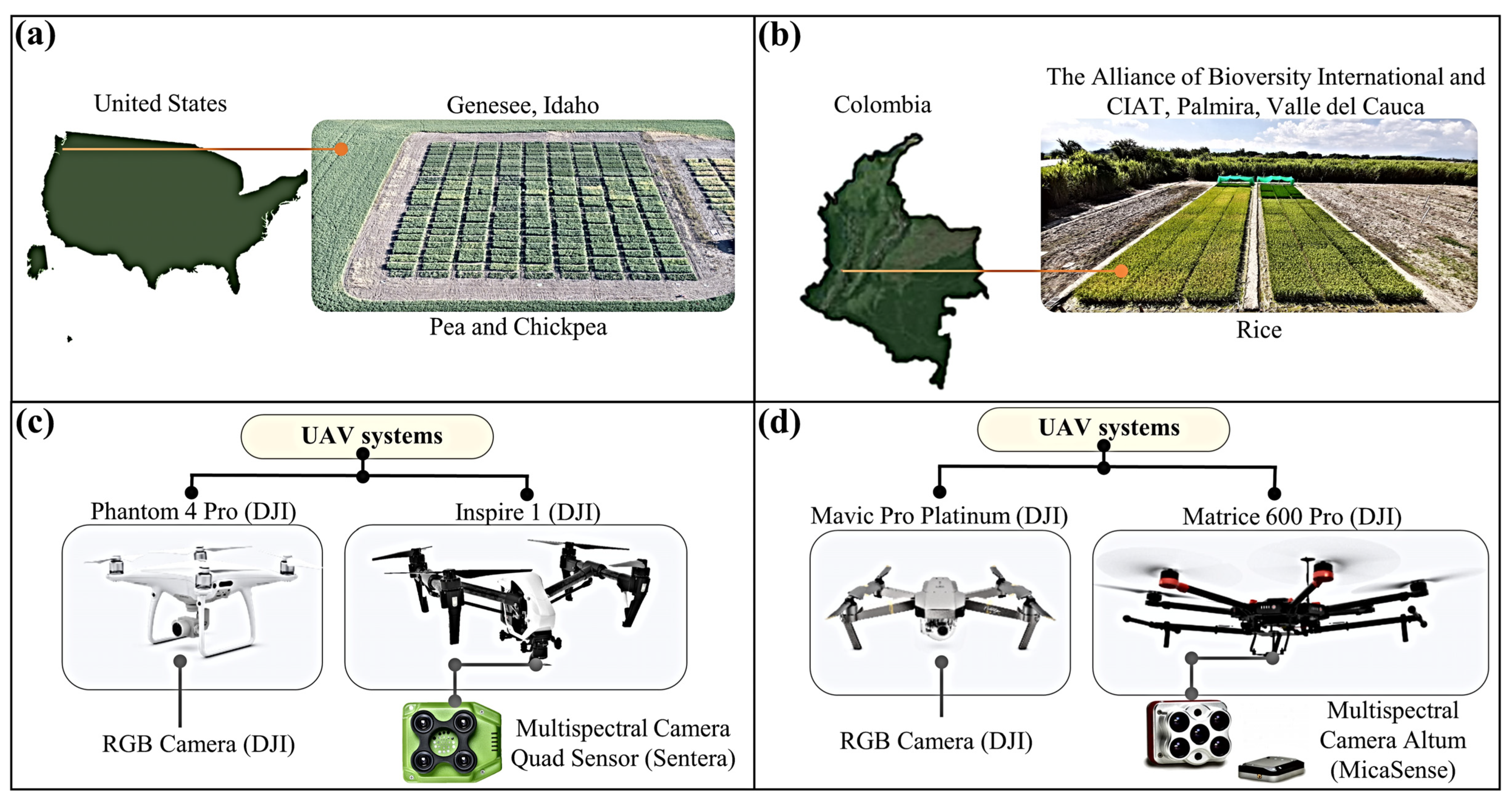
2.1. Study Locations

Four breeding trials were utilized to evaluate the effect of solar zenith angles on vegetation indices extracted from individual plots at each latitude zone. Two pulse trials were located at Genesee, Idaho, United States (representing high latitude, Figure 1a), with a continental climate, at 613.60 m above sea level (ASL, 46°36′39.92″ N−116°57′39.07″ W). The pea (Pisum sativum L.) trial contained 29 advanced green pea lines (panel 1901), and the chickpea (Cicer arietinum L.) trial (panel 1981) was comprised of 24 lines. Both trials included breeding lines and important commercial check cultivars that were arranged in a randomized complete block design with three replicates. The plots were 4.90 m × 1.50 m with 0.75 m between plots and a plant density of about 86 (peas) or 43 (chickpeas) seeds per m². The two field trials were planted on 3 May 2019. Pea and chickpea plots were harvested on 14 August and 4 September 2019, respectively. Seed treatments were as described in Zhang et al. [13].

The other two trials, paddy rice, were located at Valle del Cauca, the Alliance of Bioversity International and CIAT, Km 17 Recta Cali-Palmira, Colombia (representing low latitude, Figure 1b), with a tropical climate, at 973.80 m ASL (3°29′42.43″ N−76°21′6.80″ W). In these trials, 20 lines of rice (Oriza sativa L.), 12 lines of IR64 and eight lines of cv ‘Ciherang’, were planted on 16 May 2020, transplanted on 10 June 2020, and harvested on 25 September 2020. Rice trials were arranged in randomized block designs with four replications and plots of 2 m × 2 m. Transplanting was carried out with 20 cm between plants, 25 cm between rows, and 50 cm between plots. Agronomic management (irrigation, fertilization, and pest control) was performed in accordance with standard paddy rice production procedures.

2.2. UAV Systems and Sensors

In pulse trials, images were acquired at the early pod development stage. Our previous work [12,13] reported a strong and significant correlation between seed yield and VIs at flowering/early pod development stages. Multispectral images were acquired using a Quad Sensor (Sentera, LLC., Minneapolis, MN, USA) attached to a quadcopter UAV (DJI Inspire 1, DJI Inc., Shenzhen, China). Another quadcopter UAV (DJI Phantom 4 Pro, DJI Inc., Shenzhen, China) was utilized to capture RGB images (Figure 1c) with 20 MP resolution. The Quad Sensor used a full spectrum of RGB and 840 ± 20 nm near-infrared (NIR) bands. Both multispectral and RGB images were captured on 19 July 2019 at the following times and corresponding solar zenith angles (SZA): 06:30 (88.08°), 08:00 (73.98°), 09:00 (63.82°), 11:00 (43.58°); 13:00 (28.00°), 14:00 (25.79°), 15:30 (32.33°), and 17:00 (45.56°) (Figure 2a). UAV flights were operated with Pix4DCapture (Pix4D Inc., San Francisco, CA, USA) in a single pattern, speed of 3 m s⁻¹, 80% of horizontal and 75% vertical overlaps, sensor position of 90°, and at 50 m above ground level resulting in spatial resolution of 2.20 cm per pixel for multispectral image and 0.78 cm per pixel for RGB image. A reflectance panel (99% reflectance; Spectralon, SRS-99–120, Labsphere Inc., North Sutton, NH, USA) was applied for radiometric calibration of blue, green, and red bands, and quantum efficiency coefficients were used to estimate NIR band (Equation (1)). Subsequently, coefficient of 3.07 (e.g. 3.07 × NIR) was implemented to normalize NIR band during the computation of different vegetation indices.

$$\mathrm{NIR}=\left(2.921\times \mathrm{Blue}\right)-\left(0.754\times \mathrm{Red}\right)$$

(1)

In rice, images were acquired at the late milky stage. Our previous research [17] highlighted the milky stage as a promising phenological stage for rice grain estimation in different rice trials. Multispectral images were acquired using an Altum sensor (Altum, MicaSense Inc., Seattle, WA, USA) attached to an octocopter UAV (DJI Matrice 600, DJI Inc., Shenzhen, China) using SkyPort adapter, which allowed the operator/pilot to trigger and control the camera through the flight mission. The RGB images (12.35 MP) were captured with a quadcopter UAV (DJI Mavic Pro Platinum, DJI Inc., Shenzhen, China) (Figure 1d). The Altum sensor included five spectral channels blue, green, red, red edge, and near-infrared (with center and bandwidth of 475 ± 32, 560 ± 27, 668 ± 16, 717 ± 12, and 842 ± 57 respectively). Both multispectral and RGB images were captured on 5 September 2020, at the following times and corresponding solar zenith angles: 08:30 (53.31°), 09:30 (38.42°), 10:30 (23.56°), 12:00 (3.11°), 13:00 (14.29°), 14:00 (29.07°), and 15:00 (43.95°) (Figure 2c). UAV flight missions were created using Ground Station software (SZ DJI Technology Co. Ltd., China) in a single pattern, speed of 3 m s⁻¹, 80% of horizontal and 75% vertical overlaps, and at 45 m above ground level resulting in spatial resolution of 1.05 cm per pixel for multispectral sensor and 0.60 cm per pixel for RGB sensor. A MicaSense reflectance panel (MicaSense Inc., Seattle, WA, USA) was used to convert digital numbers into reflectance values for radiometric calibration. For all trials, light intensity data (2–4 data points per hour) and photosynthetically active radiation were collected using a quantum sensor (MQ-100, Apogee Instruments, Inc. USA) or an optical light meter (Lux-1330B, China) at different SZA to capture solar intensity at different time points (Figure 2b,d).

2.3. Ground-Truth Measurements

Seed/grain yield (GY) of both rice and pulse trials served as the primary ground-reference data. In addition, plant height (PH), tiller number (TN), and above-ground dry biomass data (DB) were acquired for rice trails. For rice, 28 plants per genotype were randomly selected (seven plants per replication), wrapped in paper bags, and taken to the seed lab. The grain and vegetative tissues (stems and leaves = biomass) were separated into independent paper bags; grain was dried to 14% of moisture, and vegetative tissues were dried for 82 h until a stable weight was obtained. Finally, grain weight, number of tillers, and weight of the vegetative tissues were recorded per plant. For pea and chickpea, the entire plot was harvested using a small plot combine to acquire seed weight. The summary statistics of agronomic traits for both pulse and rice trials are presented in

Table 1. Summary statistics of agronomic and performance traits in different trials.

Trial	Agronomic Traits	n	Min.	Max.	Median	Mean	Std. Dev.
Pea	Seed yield (kg.ha−1)	89	1665	3981	3133	3117	422
Chickpea	Seed yield (kg.ha−1)	72	1220	3205	2549	2484	394
IR64	Grain yield (g.plant−1)	36	35	61	45	45	6
	Dry biomass (g.plant−1)	36	21	38	29	29	4
	Tiller number	36	10	21	14	14	2
	Plant height (cm)	36	81	97	92	92	3
Ciherang	Grain yield (g.plant−1)	24	37	50	43	43	4
	Dry biomass (g.plant−1)	24	21	37	27	28	4
	Tiller number	24	9	13	11	11	1
	Plant height (cm)	24	88	100	94	94	3

.

2.4. Image Processing and Feature Extraction

Altum multispectral images were processed in Pix4Dmapper (Pix4D Inc., San Francisco, CA, USA) to generate rice reflectance orthomosaic using MicaSense reflectance calibration panel (MicaSense Inc., Seattle, WA, USA) with the following factors: blue × 0.519, green × 0.521, red × 0.520, red edge × 0.519, and NIR × 0.518. For vegetation indices extraction, the semi-automated image processing algorithm was developed in MATLAB (2018b; MathWorks Inc., Natick, MA, USA). The algorithms’ functions are explained in Zhang et al. [13]. In this study, nine vegetation were evaluated including NDVI [18], GNDVI [19], SAVI [20], NDRE [21], TVI [22], SR [23], OSAVI [24], NDVI_RE [25], and MCARI [26]; formulas are explained in

Table 2. UAV features applying in the study.

Image Features	Equation
Normalized Difference Vegetation Index	NDVI = (NIR − Red) / (NIR + Red)
Green Normalized Difference Vegetation Index	GNDVI = (NIR − Green) / (NIR + Green)
Soil-Adjusted Vegetation Index	SAVI = 1.5 (NIR − Red) / (NIR + Red + 0.5)
Red-Edge Normalized Difference Vegetation Index	NDRE = (NIR − RE) / (NIR + RE)
Transformed Vegetation Index	TVI = 0.5 (120 (NIR − Green) − 200 (Red − Green)
Simple Ratio	SR = NIR / Red
Optimized Soil-Adjusted Vegetation Index	OSAVI = (NIR − Red) / (NIR + Red + 0.16)
Normalized Difference Vegetation Index Red-Edge	NDVIRE= (RE − Red) / (RE + Red)
Modified Chlorophyll Absorption in Reflectance Index	MCARI = ((RED − Red) − 0.2 (RE − Green)) RE/Red
Canopy Height	CH = DSM − DTM

. These VIs were selected because they were found to indicate crop performances as reported in previous studies [12,13,17,27]. A similar process of orthomosaic generation and extraction of vegetation indices was used for pulse trails, except the extraction of indices such as NDRE, NDVI_RE, and MCARI, due to issues associated with the red-edge band.

In rice and pulse trials, RGB images were processed in Pix4Dmapper to generate digital surface models (DSM), which reported elevation data in meters above mean sea level. The topography of the terrain as Digital Terrain Model (DTM) data were created based on the interpolation of elevation data over bare soil points on DSM using open-source software Quantum Geographic Information System (QGIS) (QGIS.org, 2021, version 3.10.4). The DSM and DTM as .tif files were imported into MATLAB to calculate and extract the CH (Table 2).

2.5. Data Analysis

RStudio software [28] (Version 1.4.1106, 2021, Boston, MA) was used to evaluate the linear relationship between agronomic traits and vegetation indices using Pearson’s correlation analysis. The VI data were summarized using boxplots (Q3, median, Q1, and suspected outliers) to visualize the variability across SZA and locations. Transformation-estimating functions were used for data normalization using the bestNormalize package. Analysis of variance (ANOVA) linear model was conducted to assess the effect of SZA on VI at each location; for this model, the dependent variable score (${\mathrm{Y}}_{\mathrm{ij}}$) is expected to be the result of the added effects of the factors treatment (${\mathsf{\tau }}_{\mathrm{i}}$), block (${\mathsf{\beta }}_{\mathrm{j}}$), and error term (${\mathsf{ϵ}}_{\mathrm{ij}}$); the effects are added to the global mean (μ):

$${\mathrm{Y}}_{\mathrm{ij}}=\mathsf{\mu }+{\mathsf{\tau }}_{\mathrm{i}}+{\mathsf{\beta }}_{\mathrm{j}}+{\mathsf{ϵ}}_{\mathrm{ij}}$$

(2)

Based on the results, post-hoc pairwise comparisons (α = 0.05) of group means were performed using Tukey Honest Significant Difference (HSD) to test significant differences among SZA in each location.

3. Results

3.1. Spectral Band Analysis

Table 3. Summary statistics and ANOVA results of spectral bands across trails.

Trials	Bands	Descriptive Statistics					Post-hoc Pairwise Comparisons
		Mean	Max	Min	Range (%)	Hour	6.5	8	9	11	13	14	15.5	17
Pea	NIR	0.73	0.83	0.64	23	→	b	a	a	bc	d	bc	cd	a
	Red	0.40	0.47	0.35	26	→	c	b	b	c	d	cd	d	a
	Green	0.49	0.57	0.43	25	→	cd	a	a	a	bc	bc	d	b
	Blue	0.35	0.41	0.31	24	→	b	a	a	b	c	bc	c	a
Chickpea	NIR	0.69	0.81	0.59	27	→	e	bc	ab	d	a	cd	ac	d
	Red	0.37	0.45	0.32	29	→	d	ab	a	cd	a	bc	ab	bc
	Green	0.54	0.54	0.38	30	→	d	ab	a	c	a	c	bc	d
	Blue	0.33	0.39	0.28	28	→	e	ac	a	d	a	bcd	ab	cd
						Hour	8.5	9.5	10.5	12	13	14	15
IR64	NIR	0.37	0.47	0.30	36	→	e	d	b	a	ab	c	d
	RE	0.21	0.26	0.16	38	→	d	d	b	b	a	c	d
	Red	0.06	0.09	0.04	56	→	a	ab	bc	c	a	c	ab
	Green	0.08	0.10	0.06	40	→	e	de	b	bcd	a	bc	ce
	Blue	0.04	0.05	0.03	40	→	b	c	c	b	b	a	c
Ciherang	NIR	0.35	0.46	0.27	41	→	d	d	b	a	ab	c	d
	RE	0.17	0.21	0.14	33	→	cd	d	b	b	a	bc	cd
	Red	0.06	0.1	0.03	70	→	a	ab	cd	e	a	de	bc
	Green	0.07	0.1	0.06	40	→	ab	ab	ab	b	a	ab	ab
	Blue	0.03	0.05	0.02	60	→	a	c	c	c	bc	ab	c

shows a higher data dispersion in rice trials (33 to 70%) than pulse trials (23 to 30%). In both rice and pulse trials, a significant effect of SZA was detected (p-value < 0.0001 for all bands in all trails, except green in Ciherang, where p-value was 0.001).

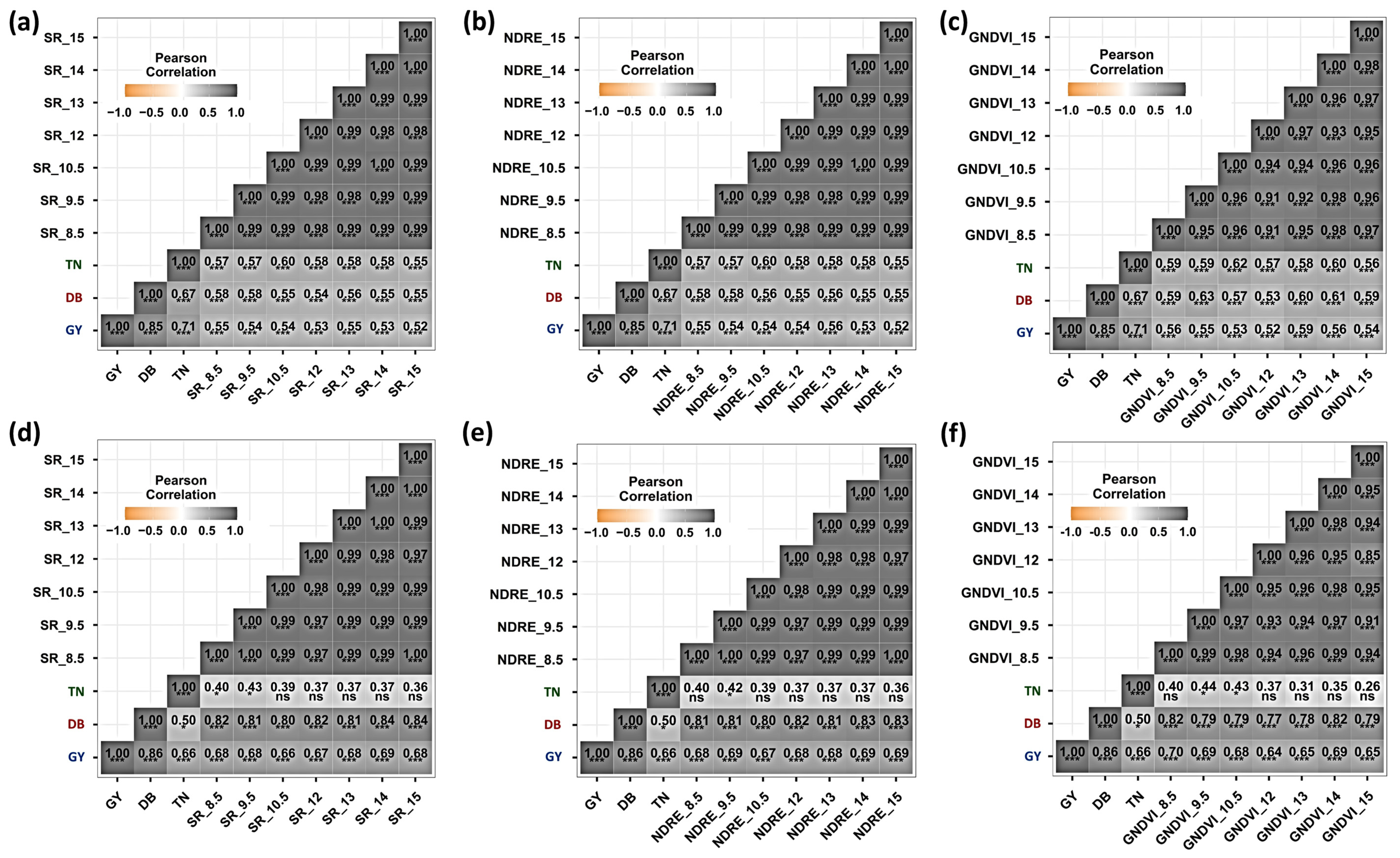
3.2. Correlation Analysis with Seed/Grain Yield

In pulse trials, Pearson’s correlation coefficients revealed that SR, OSAVI, and NDVI were statistically significant with seed yield showing some differences across SZA (Figure 3a–f). OSAVI showed low correlation (r = 0.33 and 0.28, respectively) at 09:00 (63.82°) and 13:00 (28.00°) and no significant correlation at 11:00 (43.58°) in pea. In both chickpea and pea trials, SR and NDVI displayed moderate to high significant correlations with GY (r = 0.43 to 0.69) at 11:00 and 13:00, which corresponds to 43.58° and 28.00° in the high latitude (Figure 3a,c,d,f).

In rice trials, there was a statistically significant correlation between SR, NDRE, and GNDVI and grain yield with minor differences across SZA (Figure 4a–f). The GNDVI displayed moderate to high significant correlations with GY in the IR64 (r = 0.52 to 0.59) and Ciherang lines (r = 0.64 to 0.70) across SZA as presented in Figure 4c,f. In addition, the matrix inter-correlations between SR (e.g. SR at one angle compared to SR from another angles) and NDVI for pulse lines (Figure 3a,d), and SR and GNDVI for rice trails (Figure 4c,f) at multiple SZA, were between 0.74 to 0.99, which indicated stability across SZA. Figure 5 shows correlation plots between SR or GNDVI with GY for chickpea, pea, and rice plots across SZA. The correlation with seed/grain yield and other agronomic traits are summarized in Supplementary materials, Figures S1–S4.

3.3. Correlation Analysis with Dry Biomass and Tiller Number

Biomass (the vegetative tissues) is a reliable indicator of rice production, thus, a strong correlation (r = 0.85 to 0.86, p ≤ 0.001) between rice grain yield and dry biomass was observed. Pearson correlation demonstrated that SR, NDRE, and GNDVI showed stable and highly significant correlations (p-values ≤ 0.001) in both trials with dry biomass across SZA (Figure 4a–f). For the IR64 lines, VIs displayed a good correlation (Figure 4c) with biomass, while for the Ciherang lines, a higher correlation (Figure 4d) with biomass was observed, especially with SR. The relationship among SZA between tiller number and VI indicated a significantly moderate correlation with SR, NDRE, and GNDVI in the IR64 lines (Figure 4a–c). In contrast, TVI showed the best correlation (r = 0.46 to 0.55) with the tiller numbers for the Ciherang lines (Supplementary materials, Figure S3d).

3.4. Correlation Analysis with Plant Height

Table 4. Correlation coefficient between UAV-based plant height estimate with ground-truth references and VIs at different SZA.

Time (h)		6.5	8	9	11	13	14	15.5	17		8.5	9.5	10.5	12	13	14	15
Pea	PH	-	-	-	-	-	-	-		IR64	0.65 ***	0.60 ***	0.61 ***	0.59 ***	0.54 ***	0.61 ***	0.60 ***
	GY	0.38 ***	0.42 ***	0.39 ***	0.39 ***	0.33 **	0.33 **	0.32 **	0.32 **		0.48 **	0.50 **	0.5 **	0.43 **	0.43 **	0.47 **	0.48 **
	DB	-	-	-	-	-	-	-			0.45 **	0.44 **	0.43 **	0.40 *	0.42 *	0.42 **	0.44 **
	TN	-	-	-	-	-	-	-			0.22 NS	0.21 NS	0.21 NS	0.15 NS	0.16 NS	0.20 NS	0.20 NS
	NDVI	0.49 ***	0.53 ***	0.56 ***	0.58 ***	0.54 ***	0.53 ***	0.48 ***	0.28 **		0.39 *	0.40 *	0.36 *	0.39 *	0.15 NS	0.28 NS	0.42 *
	GNDVI	0.48 ***	0.46 ***	0.45 ***	0.45 ***	0.43 ***	0.47 ***	0.44 ***	0.29 **		0.39 *	0.37 *	0.32 NS	0.34 *	0.40 *	0.43 **	0.42 *
	SAVI	0.48 ***	0.33 **	0.21 NS	0.05 NS	0.05 NS	0.07 NS	0.30 **	0.25 *		0.38 *	0.36 *	0.36 *	0.29 NS	0.07 NS	0.33 *	0.44 **
	NDRE	-	-	-	-	-	-	-			0.50 **	0.48 **	0.42 **	0.43 **	0.43 **	0.51 ***	0.47 **
	TVI	0.49 ***	0.53 ***	0.56 ***	0.58 ***	0.54 ***	0.52 ***	0.48 ***	0.28 **		0.36 *	0.33 *	0.35 *	0.23 NS	−0.03 NS	0.3 NS	0.43 **
	SR	0.37 ***	0.10 NS	−0.14 NS	−0.28 **	−0.31 **	−0.24 *	0.04 NS	0.14 NS		0.52 ***	0.49 **	0.44 **	0.44 **	0.44 **	0.53 ***	0.48 **
	OSAVI	0.46 ***	0.28 **	0.13 NS	−0.05 NS	−0.05 NS	−0.01 NS	0.25 *	0.23 *		0.39 *	0.38 *	0.37 *	0.34 *	0.11 NS	0.32 NS	0.44 **
	NDVIRE	-	-	-	-	-	-	-			0.31 NS	0.33 *	0.26 NS	0.31 NS	−0.04 NS	0.09 NS	0.34 *
	MCARI	-	-	-	-	-	-	-			0.43 **	0.40 *	0.38 *	0.33 NS	0.28 NS	0.44 **	0.47 **
Chickpea	PH	-	-	-	-	-	-	-		Ciherang	0.85 ***	0.86 ***	0.83 ***	0.75 ***	0.83 ***	0.82 ***	0.75 ***
	GY	0.26 *	0.39 ***	0.57 ***	0.63 ***	0.49 ***	0.26 *	0.21 NS	0.16 NS		0.45 *	0.28 NS	0.39 NS	0.21 NS	0.37 NS	0.45 *	0.27 NS
	DB	-	-	-	-	-	-	-			0.66 ***	0.51 *	0.64 ***	0.44 *	0.58 **	0.70 ***	0.54 **
	TN	-	-	-	-	-	-	-			−0.02 NS	−0.17 NS	−0.08 NS	−0.27 NS	−0.09 NS	−0.05 NS	−0.24 NS
	NDVI	0.45 ***	0.55 ***	0.63 ***	0.75 ***	0.62 ***	0.41 ***	0.31 **	0.29 *		0.43 *	0.14 NS	0.29 NS	0.03 NS	0.45 *	0.32 NS	0.38 NS
	GNDVI	0.49 ***	0.49 ***	0.43 ***	0.54 ***	0.49 ***	0.42 ***	0.39 ***	0.33 **		0.66 ***	0.42 *	0.60 **	0.32 NS	0.65 ***	0.64 ***	0.63 ***
	SAVI	0.30 **	0.28 *	0.07 NS	0.16 NS	0.09 NS	0.23 NS	0.28 *	0.29 *		0.53 **	0.28 NS	0.37 NS	0.07 NS	0.48 *	0.40 NS	0.38 NS
	NDRE	-	-	-	-	-	-	-			0.67 ***	0.47 *	0.63 ***	0.38 NS	0.62 ***	0.65 ***	0.51 **
	TVI	0.45 ***	0.54 ***	0.62 ***	0.74 ***	0.62 ***	0.41 ***	0.30 **	0.27 *		0.51 **	0.28 NS	0.34 NS	<0.01 NS	0.44 *	0.37 NS	0.33 NS
	SR	0.10 NS	0.15 NS	−0.12 NS	−0.06 NS	−0.06 NS	0.05 NS	0.13 NS	0.19 NS		0.66 ***	0.46 *	0.63 ***	0.37 NS	0.61 **	0.64 ***	0.50 *
	OSAVI	0.48 ***	0.49 ***	0.53 ***	0.69 ***	0.55 ***	0.43 ***	0.35 **	0.31 **		0.50 *	0.22 NS	0.34 NS	0.05 NS	0.47 *	0.37 NS	0.39 NS
	NDVIRE	-	-	-	-	-	-	-			0.2 NS	−0.15 NS	−0.01 NS	−0.29 NS	0.29 NS	−0.03 NS	0.18 NS
	MCARI	-	-	-	-	-	-	-			0.61 **	0.37 NS	0.51 **	0.21 NS	0.57 **	0.55 **	0.51 *

Statistical significance: p > 0.05 (ns); p ≤ 0.05 (*); p ≤ 0.01 (**); p ≤ 0.001 (***); and Not significant (^NS).

presents the correlations between UAV-based plant height estimates and ground-truth reference data and VIs across SZA. In pulses, NDVI, GNDVI, and TVI showed a significant correlation with plant height data across most SZA. The highly significant correlations (p-values ≤ 0.001) for plant height were found in pulses at 09:00 (63.82°), 11:00 (43.80°), and 13:00 h (28.00°) with NDVI. Moderate to a high correlation between measured and estimated plant height was observed for the IR64 and Ciherang trials across SZA. For the rice trials, except for Ciherang at noon (3.11°), NDRE and SR demonstrated a significant correlation with plant height across SZA. Based on ANOVA analysis, there was the SZA effect (p-values ≤ 0.0001); however, the post-hoc test indicated reasonable stability in data acquired at most SZA (Figure 6a–c).

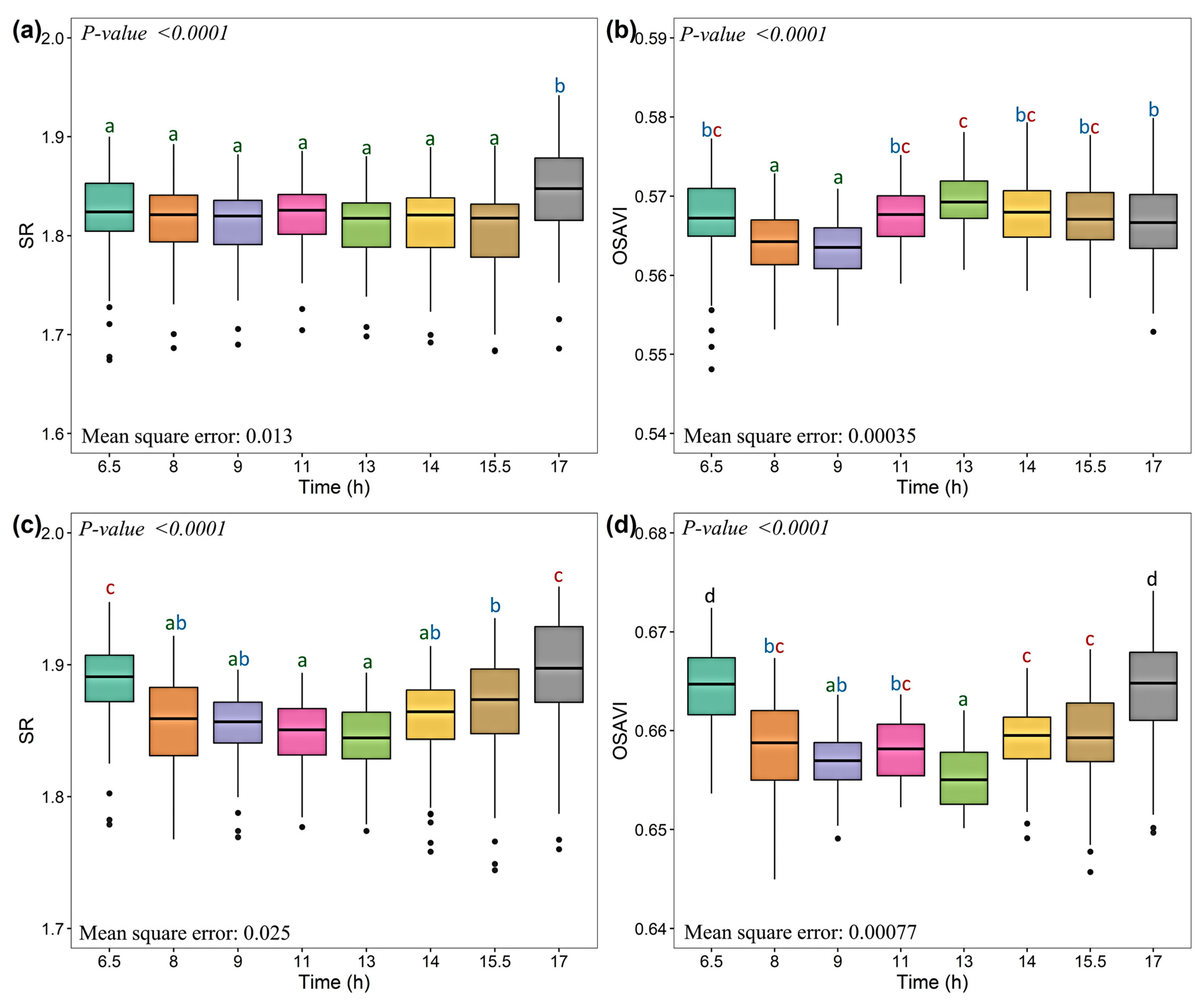
3.5. Influence of SZA Based on Analysis of Variance and Post-Hoc Test

The VI data that were substantially correlated with grain yield were selected to perform the ANOVA across SZA. The mean differences of SR, OSAVI, NDRE, and GNDVI across SZA and locations (p-values ≤ 0.0001) strongly indicated that the mean of at least one group significantly differed from other groups (Figure 7, Figure 8 and Figure 9). This indicates that the Lambertian property may not be present on the VI acquired from pulse and rice crop surfaces. Tukey’s multiple comparison test showed the different groups (Figure 7, Figure 8 and Figure 9). SR and OSAVI were used for pulse trials for this test, while NDRE, GNDVI, and SR were used for rice trials. In pulse trails, in comparison to the SR, OSAVI showed more variation across SZA (Figure 7); indicating a more anisotropic effect on OSAVI associated with solar view angles, especially when the images were captured at the earlier and later times (Figure 7b, d); however, OSAVI showed low mean square error (0.00035 to 0.00077). This comparison indicates that SR can be measured over a broader solar zenith angle range, 08:00 h (73.98°) to 14:00 h (25.79°) (Figure 7a,c), Tukey test analysis on NDRE, GNDVI, and SR of the IR64 lines also showed statistically different groups among solar view angles; in general, noontime had low VI values across SZA. GNDVI had the highest values at early and late time points (Figure 8c,d). We observed that trends of NDRE and SR indices at most SZA were similar, except at 12:00 (3.11°) and 14:00 (29.07°) (Figure 9a,e). In contrast, NDRE and SR over the Ciherang lines revealed few groups compared to the IR64 lines. This result indicates that the VI values were statistically similar across SZAs (Figure 9a,e). Based on this, we can infer the minimum anisotropic effect.

4. Discussion

The models developed to estimate BDRF are found to offer robust and effective compensation of reflectance anisotropic [4,8]. Nevertheless, such measurements can still be challenging due to data accuracy [4] and parameter selection [8], in addition to variability within the crop. In this study, we evaluated the performance of some of the VI widely used for plant breeding to identify VI that may not need anisotropic correction. As expected, we found the effects of the SZA on SR, OSAVI, NDRE, and GNDVI at both high and low latitudes (Figure 8 and Figure 9). In the tallgrass prairie, Middleton [29] reported significant dependence of SR and NDVI on the SZA. In this study, the variation caused by the SZA was found to be the least for SR and the greatest for other VI in high and low latitudes. This result is supported by Hashimoto et al. [30], who simulated the reflectance on the rice paddy field, indicating the least saturation of SR compared with NDVI. Ma et al. [31] found that the NDVI data extracted from savanna were more sensitive than enhanced vegetation index (EVI) to the SZA effects. Since the absolute VI data is affected by the SZA, the data need to be standardized prior to the use of such data in crop models and similar applications. Moreover, consistency during data acquisition should be maintained for proper interpretation of the data. The VI data that is independent of the anisotropic reflectance effect may also be used to create stable datasets. Nevertheless, further validation is needed across crops, phenological stages, and latitudes to explore these solutions. Middleton [29] and Ishihara [32] found varied results when assessing VIs data extracted from imagery from prairie and croplands.

In addition to a stable correlation between SR and GY across SZA, a very strong correlation between SR data at different SZA was found in this study. Naito et al. [16] reported a similarly strong correlation between SR and GY in paddy rice as well, based on data collected around noon. Even though SR, OSAVI, NDRE, and GNDVI data were statistically different across SZA, they showed a stable correlation with grain yield. In general, SR data exhibited low variability (mean square error = 0.013 to 0.37) and better consistency. Similar results were found with NDRE data, especially for Ciherang rice lines. Based on the correlation analysis with seed/grain yield, the results indicate that for phenotyping applications in crop breeding programs, where relative differences between crop performance across different varieties are evaluated, multiple vegetation indices can be utilized, even if there are differences in the SZA during data acquisition. Although the results are encouraging, further validation across breeding programs is needed. Moreover, standardization of data acquisition is necessary to develop crop growth and development curves using remote sensing data.

5. Conclusions

In this study, we found that the evaluated vegetation indices are significantly affected by different SZAs. There were two major findings: (1) The evaluated VIs maintained a consistent correlation with seed/grain yield in all four trials at both latitudes (low and high). The evaluated vegetation indices can be applicable for phenotyping applications in breeding programs to study the relative differences between crop varieties; and (2) based on the analysis to find the best VI with minimum bidirectional effect (low variance) and high correlation with grain yield across SZAs, SR was identified. Thus, SR has the potential as a yield indicator or predictor across solar zenith angles for a wide range of remote sensing applications without anisotropic reflectance correction.

Nevertheless, further work is needed, using different crops, phenological stages, latitudes, and different sensor angles. Such research will be useful to further validate the findings from this study and identify similar/different vegetation indices with minimum anisotropic reflectance effect, allowing image acquisition across broader solar zenith angles, which is essential for the interpretation of images in precision agriculture and crop modeling applications.

References

1. Ustin, S.L.; Jacquemoud, S. How the optical properties of leaves modify the absorption and scattering of energy and enhance leaf functionality? In Remote Sensing of Plant Biodiversity; Springer International Publishing: Cham, Switzerland, 2020; pp. 349–384. [Google Scholar]
2. Goodin, D.G.; Gao, J.; Henebry, G.M. The effect of solar illumination angle and sensor view angle on observed patterns of spatial structure in tallgrass prairie. IEEE Trans. Geosci. Remote Sens. 2004, 42, 154–165. [Google Scholar] [CrossRef]
3. Wen, J.; Liu, Q.; Xiao, Q.; Liu, Q.; You, D.; Hao, D.; Wu, S.; Lin, X. Characterizing land surface anisotropic reflectance over rugged terrain: A review of concepts and recent developments. Remote Sens. 2018, 10, 370. [Google Scholar] [CrossRef] [Green Version]
4. Wierzbicki, D.; Kedzierski, M.; Fryskowska, A.; Jasinski, J. Quality assessment of the bidirectional reflectance distribution function for NIR imagery sequences from UAV. Remote Sens. 2018, 10, 1348. [Google Scholar] [CrossRef] [Green Version]
5. Weyermann, J.; Damm, A.; Kneubuhler, M.; Schaepman, M.E. Correction of reflectance anisotropy effects of vegetation on airborne spectroscopy data and derived products. IEEE Trans. Geosci. Remote Sens. 2014, 52, 616–627. [Google Scholar] [CrossRef]
6. Latifovic, R.; Cihlar, J.; Chen, J. A comparison of BRDF models for the normalization of satellite optical data to a standard sun-target-sensor geometry. IEEE Trans. Geosci. Remote Sens. 2003, 41, 1889–1898. [Google Scholar] [CrossRef]
7. Renhorn, I.G.E.; Hallberg, T.; Boreman, G.D. Efficient polarimetric BRDF model. Opt. Express 2015, 23, 31253–31273. [Google Scholar] [CrossRef]
8. Susaki, J.; Hara, K.; Kajiwara, K.; Honda, Y. Robust estimation of BRDF model parameters. Remote Sens. Environ. 2004, 89, 63–71. [Google Scholar] [CrossRef]
9. Doering, D.; Vizzotto, M.R.; Bredemeier, C.; da Costa, C.M.; Henriques, R.V.B.; Pignaton, E.; Pereira, C.E. MDE-based development of a multispectral camera for precision agriculture. IFAC-Pap. 2016, 49, 24–29. [Google Scholar] [CrossRef]
10. Yang, G.; Liu, J.; Zhao, C.; Li, Z.; Huang, Y.; Yu, H.; Xu, B.; Yang, X.; Zhu, D.; Zhang, X.; et al. Unmanned Aerial Vehicle Remote Sensing for Field-Based Crop Phenotyping: Current Status and Perspectives. Front. Plant Sci. 2017, 8, 1111. [Google Scholar] [CrossRef]
11. Ahmed, I.; Eramian, M.; Ovsyannikov, I.; van der Kamp, W.; Nielsen, K.; Duddu, H.S.; Rumali, A.; Shirtliffe, S.; Bett, K. Automatic detection and segmentation of lentil crop breeding plots from multi-spectral images captured by UAV-mounted camera. In Proceedings of the 2019 IEEE Winter Conference on Applications of Computer Vision (WACV), Waikoloa Village, HI, USA, 7–11 January 2019; pp. 1673–1681. [Google Scholar]
12. Quirós, J.J.; McGee, R.J.; Vandemark, G.J.; Romanelli, T.; Sankaran, S. Field phenotyping using multispectral imaging in pea (Pisum aativum L) and chickpea (Cicer arietinum L). Eng. Agric. Environ. Food 2019, 12, 404–413. [Google Scholar] [CrossRef]
13. Zhang, C.; McGee, R.J.; Vandemark, G.J.; Sankaran, S. Crop performance evaluation of chickpea and dry pea breeding lines across seasons and locations using phenomics data. Front. Plant Sci. 2011, 12, 61. [Google Scholar]
14. Zhang, C.; Craine, W.A.; McGee, R.J.; Vandemark, G.J.; Davis, J.B.; Brown, J.; Hulbert, S.H.; Sankaran, S. Image-based phenotyping of flowering intensity in cool-season crops. Sensors 2020, 20, 1450. [Google Scholar] [CrossRef] [Green Version]
15. Kang, Y.; Nam, J.; Kim, Y.; Lee, S.; Seong, D.; Jang, S.; Ryu, C. Assessment of regression models for predicting rice yield and protein content using unmanned aerial vehicle-based multispectral imagery. Remote Sens. 2021, 13, 1508. [Google Scholar] [CrossRef]
16. Ogawa, D.; Sakamoto, T.; Tsunematsu, H.; Kanno, N.; Nonoue, Y.; Yonemaru, J.-I. Haplotype analysis from unmanned aerial vehicle imagery of rice MAGIC population for the trait dissection of biomass and plant architecture. J. Exp. Bot. 2021, 72, 2371–2382. [Google Scholar] [CrossRef]
17. Naito, H.; Ogawa, S.; Valencia, M.O.; Mohri, H.; Urano, Y.; Hosoi, F.; Shimizu, Y.; Chavez, A.L.; Ishitani, M.; Selvaraj, M.G.; et al. Estimating rice yield related traits and quantitative trait loci analysis under different nitrogen treatments using a simple tower-based field phenotyping system with modified single-lens reflex cameras. ISPRS J. Photogramm. Remote Sens. 2017, 125, 50–62. [Google Scholar] [CrossRef]
18. Rouse, J.; Haas, R.H.; Deering, D.; Schell, J.A.; Harlan, J. Monitoring the Vernal Advancement and Retrogradation (Green Wave Effect) of Natural Vegetation; NASA/GSFC Type III Final Report; Texas A&M University: Greenbelt, MD, USA, 1974; p. 371. [Google Scholar]
19. Gitelson, A.A.; Kaufman, Y.J.; Merzlyak, M.N. Use of a green channel in remote sensing of global vegetation from EOS-MODIS. Remote Sens. Environ. 1996, 58, 289–298. [Google Scholar] [CrossRef]
20. Huete, A.R. A soil-adjusted vegetation index (SAVI). Remote Sens. Environ. 1988, 25, 295–309. [Google Scholar] [CrossRef]
21. Gitelson, A.; Merzlyak, M.N. Spectral reflectance changes associated with autumn senescence of Aesculus hippocastanum L. and Acer platanoides L. leaves. Spectral features and relation to chlorophyll estimation. J. Plant Physiol. 1994, 143, 286–292. [Google Scholar] [CrossRef]
22. Deering, D.W.; Rouse, J.W.; Haas, R.H.; Schel, J.A. Measuring forage production of grazing units from landsat mss data. In Proceedings of the 10th International Symposium of Remote Sensing of Environment, Ann Arbor, MI, USA, 6–10 October 1975; Volume II, pp. 1169–1178. [Google Scholar]
23. Birth, G.S.; McVey, G.R. Measuring the color of growing turf with a reflectance spectrophotometer 1. Agron. J. 1968, 60, 640–643. [Google Scholar] [CrossRef]
24. Rondeaux, G.; Steven, M.; Baret, F. Optimization of soil-adjusted vegetation indices. Remote Sens. Environ. 1996, 55, 95–107. [Google Scholar] [CrossRef]
25. Delegido, J.; Verrelst, J.; Alonso, L.; Moreno, J. Evaluation of Sentinel-2 Red-Edge Bands for Empirical Estimation of Green LAI and Chlorophyll Content. Sensors 2011, 11, 7063–7081. [Google Scholar] [CrossRef] [PubMed] [Green Version]
26. Daughtry, C.; Walthall, C.; Kim, M.; Brownde de Colstoun, E.; McMurtrey, J. Estimating corn leaf chlorophyll concentration from leaf and canopy reflectance. Remote Sens. Environ. 2000, 74, 229–239. [Google Scholar] [CrossRef]
27. Zhang, K.; Ge, X.; Shen, P.; Li, W.; Liu, X.; Cao, Q.; Zhu, Y.; Cao, W.; Tian, Y. Predicting rice grain yield based on dynamic changes in vegetation indexes during early to mid-growth stages. Remote Sens. 2019, 11, 387. [Google Scholar] [CrossRef] [Green Version]
28. RStudio Team. RStudio: Integrated Development Environment for R. RStudio; PBC: Boston, MA, USA, 2021; Available online: http://www.rstudio.com/ (accessed on 4 March 2021).
29. Middleton, E. Solar zenith angle effects on vegetation indices in tallgrass prairie. Remote Sens. Environ. 1991, 38, 45–62. [Google Scholar] [CrossRef]
30. Hashimoto, N.; Saito, Y.; Maki, M.; Homma, K. Simulation of reflectance and vegetation indices for unmanned aerial vehicle (UAV) monitoring of paddy fields. Remote Sens. 2019, 11, 2119. [Google Scholar] [CrossRef] [Green Version]
31. Ma, X.; Huete, A.; Tran, N.N. Interaction of seasonal sun-angle and savanna phenology observed and modelled using MODIS. Remote Sens. 2019, 11, 1398. [Google Scholar] [CrossRef] [Green Version]
32. Ishihara, M.; Inoue, Y.; Ono, K.; Shimizu, M.; Matsuura, S. The impact of sunlight conditions on the consistency of vegetation indices in croplands—Effective usage of vegetation indices from continuous ground-based spectral measurements. Remote Sens. 2015, 7, 14079. [Google Scholar] [CrossRef] [Green Version]
Figure 1. Locations and UAV sensor systems used in this study: (a,c) Genesee, Idaho; (b,d) Km 17 Recta Cali-Palmira, Colombia.
Drones 05 00080 g001
Figure 2. Images acquisition at different solar zenith angles and light conditions: (a,b) Genesee, Idaho; (c,d) Km 17 Recta Cali-Palmira, Colombia.
Drones 05 00080 g002
Figure 3. Pearson correlation coefficient between grain yield (GY) and simple ratio (SR), optimized soil-adjusted vegetation index (OSAVI), and normalized difference vegetation index (NDVI) across SZA [06:30 (88.08°), 08:00 (73.98°), 09:00 (63.82°), 11:00 (43.50°); 13:00 (28.00°), 14:00 (25.79°), and 15:30 (32.33°)]: (ac) pea and (df) chickpea. Statistical significance: p > 0.05 (ns); p ≤ 0.05 (*); p ≤ 0.01 (**); p ≤ 0.001 (***); and Not significant (ns).
Drones 05 00080 g003
Figure 4. Pearson correlation coefficient between grain yield (GY) and simple ratio (SR), red-edge normalized difference vegetation index (NDRE) and green normalized difference vegetation index (GNDVI) across solar zenith angles [08:30 (53.31°), 09:30 (38.42°), 10:30 (23.56°), 12:00 (3.11°), 13:00 (14.29°), 14:00 (29.07°), and 15:00 (43.95°)]: (ac) IR64 lines and (df) Ciherang lines. Statistical significance: p > 0.05 (ns); p ≤ 0.05 (*); p ≤ 0.01 (**); p ≤ 0.001 (***); and Not significant (ns).
Drones 05 00080 g004
Figure 5. Scatter plots showing the relationship between vegetation indices and seed/grain yield across solar zenith angles: (a) pea, (b) chickpea, (d) IR64, and (c) Ciherang lines.
Drones 05 00080 g005
Figure 6. One-way ANOVA and post-hoc Tukey’s honest significant difference test comparing estimated plant height across the solar zenith angles: (a) pea; (b) chickpea, (c) IR64 (rice); and (d) Ciherang (rice) lines. The same letter indicates statistically non-significant differences between the mean values.
Drones 05 00080 g006
Figure 7. One-way ANOVA and post-hoc Tukey’s honest significant difference test comparing VI across the solar zenith angles: (a,b) pea; (c,d) chickpea. The same letter indicates statistically non-significant differences between the mean values of the corresponding VI.
Drones 05 00080 g007
Figure 8. One-way ANOVA and post-hoc Tukey’s honest significant difference test comparing VI across the solar zenith angles in IR64 lines. The same letter indicates statistically non-significant differences between the mean values of the corresponding VI. (a,b) NDRE, (c,d) GNDVI, (e,f) SR.
Drones 05 00080 g008
Figure 9. One-way ANOVA and post-hoc Tukey’s honest significant difference test comparing VI across the solar zenith angles in Ciherang lines. The same letter indicates statistically non-significant differences between the mean values of the corresponding VI. (a,b) NDRE, (c,d) GNDVI, (e,f) SR.
Drones 05 00080 g009