Article

Propeller Position Effects over the Pressure and Friction Coefficients over the Wing of an UAV with Distributed Electric Propulsion: A Proper Orthogonal Decomposition Analysis

CMT—Motores Térmicos, Universitat Politècnica de València, Camino de Vera s/n, 46022 Valencia, Spain
*
Author to whom correspondence should be addressed.
Submission received: 15 December 2021 / Revised: 25 January 2022 / Accepted: 26 January 2022 / Published: 29 January 2022
(This article belongs to the Special Issue Feature Papers of Drones)

Abstract

:
New propulsive architectures, with high interactions with the aerodynamic performance of the platform, are an attractive option for reducing the power consumption, increasing the resilience, reducing the noise and improving the handling of fixed-wing unmanned air vehicles. Distributed electric propulsion with boundary layer ingestion over the wing introduces extra complexity to the design of these systems, and extensive simulation and experimental campaigns are needed to fully understand the flow behaviour around the aircraft. This work studies the effect of different combinations of propeller positions and angles of attack over the pressure coefficient and skin friction coefficient distributions over the wing of a 25 kg fixed-wing remotely piloted aircraft. To get more information about the main trends, a proper orthogonal decomposition of the coefficient distributions is performed, which may be even used to interpolate the results to non-simulated combinations, giving more information than an interpolation of the main aerodynamic coefficients such as the lift, drag or pitching moment coefficients.

1. Introduction

The requirement of more efficient and environmentally-friendly unmanned air vehicles (UAVs) is a necessity, as expressed by the National Aeronautics and Space Administration (NASA) in its Environmentally Responsible Aviation (ERA) project that is included in the information Technology Development Solutions (ITDS) [1]. The growth prevision of the global UAV fleet is alarmingly high in the coming years, as shown by the study by the Boston Consulting Group (BCG) [2], where it is estimated that in the year 2050 the fleet of industrial drones in Europe and the United States will exceed one million units.
In recent years, the application of novel technologies has been studied to achieve a higher aerodynamically and propulsively efficient aircraft, in a quest to develop aircraft with less fuel and energy consumption and less pollutant and greenhouse gas emissions.
One of these technologies is distributed electrical propulsion (DEP), which consists of the allocation of the total power required by the aircraft in different propulsive systems throughout the wingspan. This distribution has reported important advantages compared to a classic small aircraft configuration, normally relegated to the use of a single propeller. These benefits include resilience against foreign object damage [3], propulsive efficiency improvements (as the total area swept by the propellers can be increased over what can be done for a few-propellers configurations) [4], noise reduction and spectrum alteration [5,6], improved aerodynamic efficiency by vorticity control and vectored thrust [7,8] or more wing structural stability [9].
The use of DEP in high-weight UAVs is possible thanks to the use of hybrid electric propulsive plants, being this technology widely studied, since by itself it provides advantages from the point of view of fuel economy and related polluting emissions [10,11]
The proper use of DEP is strongly dependent on a correct optimisation of the location of the engines as studied in [5]. If the propulsion plant is placed in front of the wing, the increased lift generated by the propellers at the washed area of the wing allows gaining control authority. However, If the propulsion plant is located behind the wing i.e., near the trailing edge, it is possible to take advantage of the boundary layer formed on the wing to increase both the propulsive efficiency of the engine and the aerodynamic efficiency of the wing. This phenomenon is known as boundary layer ingestion (BLI). BLI’s application is based, on the one hand, on reducing the intake speed of the air that the engine ingests, so that it needs less power to produce the same thrust, as described by Budziszewski in [12]. On the other hand, as pointed out in the work of Teperin et al. and Hall et al. [13,14,15], the ingestion could reduce the lift-induced drag enough to increase aerodynamic efficiency even though the skin friction drag increases due to the re-acceleration.
In this work, an analysis of the pressure and friction coefficients of an aircraft with DEP and BLI will be carried out using computational fluid dynamics (CFD) and proper orthogonal decomposition (POD), a tool that seeks to simplify a complex problem into a series of simpler deterministic functions, allowing the creation of models that facilitate the design.
POD is historically used in fluid mechanics problems, both experimental and numerical, although it has also been used in many other engineering processes in order to always extract dominant characteristics and trends. Some recent studies where the application of POD in fluid fields can be seen are the investigation of Broatch et al. [16] where this tool is used to analyse acoustic fields in radial compressors, or the work of Torregrosa et al. [17] where the modal decomposition helps to characterise the unsteady flow field of a combustion chamber. Like the last study, it is easy to find the application of POD in the field of thermal engines [18,19,20], but this method is also used to analyse different aerodynamic problems. These include the interpolation of transonic flows [21], the creation of reduced-order models to characterise aircraft flying at high angles of attack [22], or to generate three-dimensional flow models for supersonic aircraft that significantly reduces the need of computationally-expensive high fidelity simulations [23].
The final goal of POD is the decomposition of a space vector into a series of deterministic spatial functions that are modulated through a series of configuration coefficients. Each one of the spatial functions is orthonormal with respect to the others, so they will be independent since their vector product is null. It is possible to order these functions according to what percentage of the problem they explain, which is known as total fluctuating kinetic energy ( TKE ).
The main contribution of the current research paper is the analysis of the effects that the propeller position of an fixed-wing UAV with DEP and BLI induce into the pressure and friction coefficients over its wings. This coefficients were obtained by means of computational fluid dynamics (CFD) simulations, and a modal decomposition by means of POD was performed on that data. The main trends are observed, including the movement of laminar transitional bubbles, changes in the suction peak near the leading edge or reductions and increases in the skin friction coefficient near the trailing edge, all as a function of the propeller positions at different angles of attack. By using the modal decomposition results, it is also possible to interpolate the pressure coefficient and the friction coefficient to non-simulated conditions, thus obtaining more detailed information than just interpolating global aerodynamic coefficients such as the lift or the drag coefficients.
The document is organised as follows. First, in Section 2, the aircraft analysed in this work is described. Then, in Section 3, the main methods and models are presented, explaining both the CFD and the POD approaches. In Section 4, the modal decomposition results for different propeller positions and angles of attack are shown and discussed. Finally, all main results and discussions are summarised in the conclusions in Section 5.

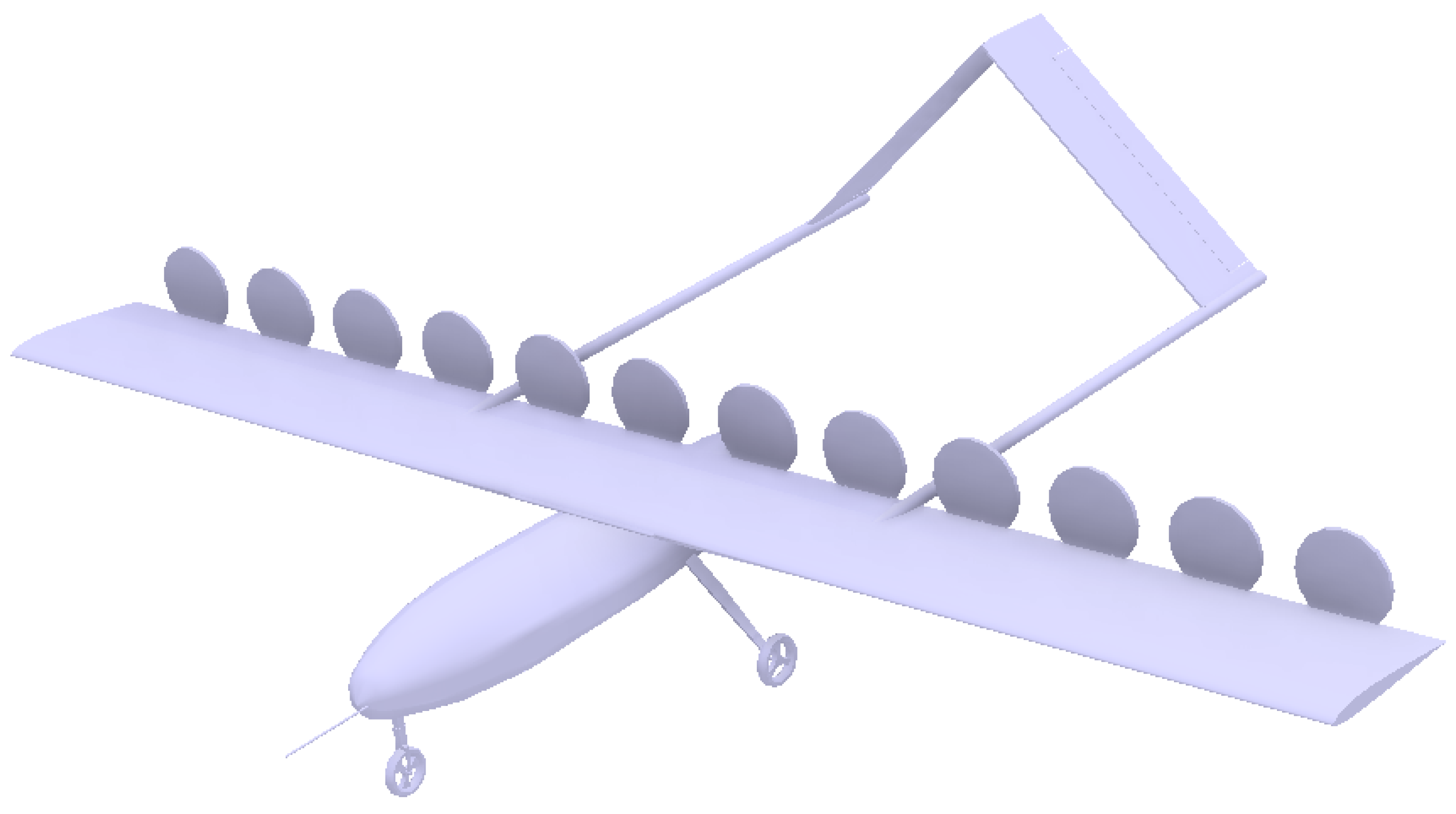
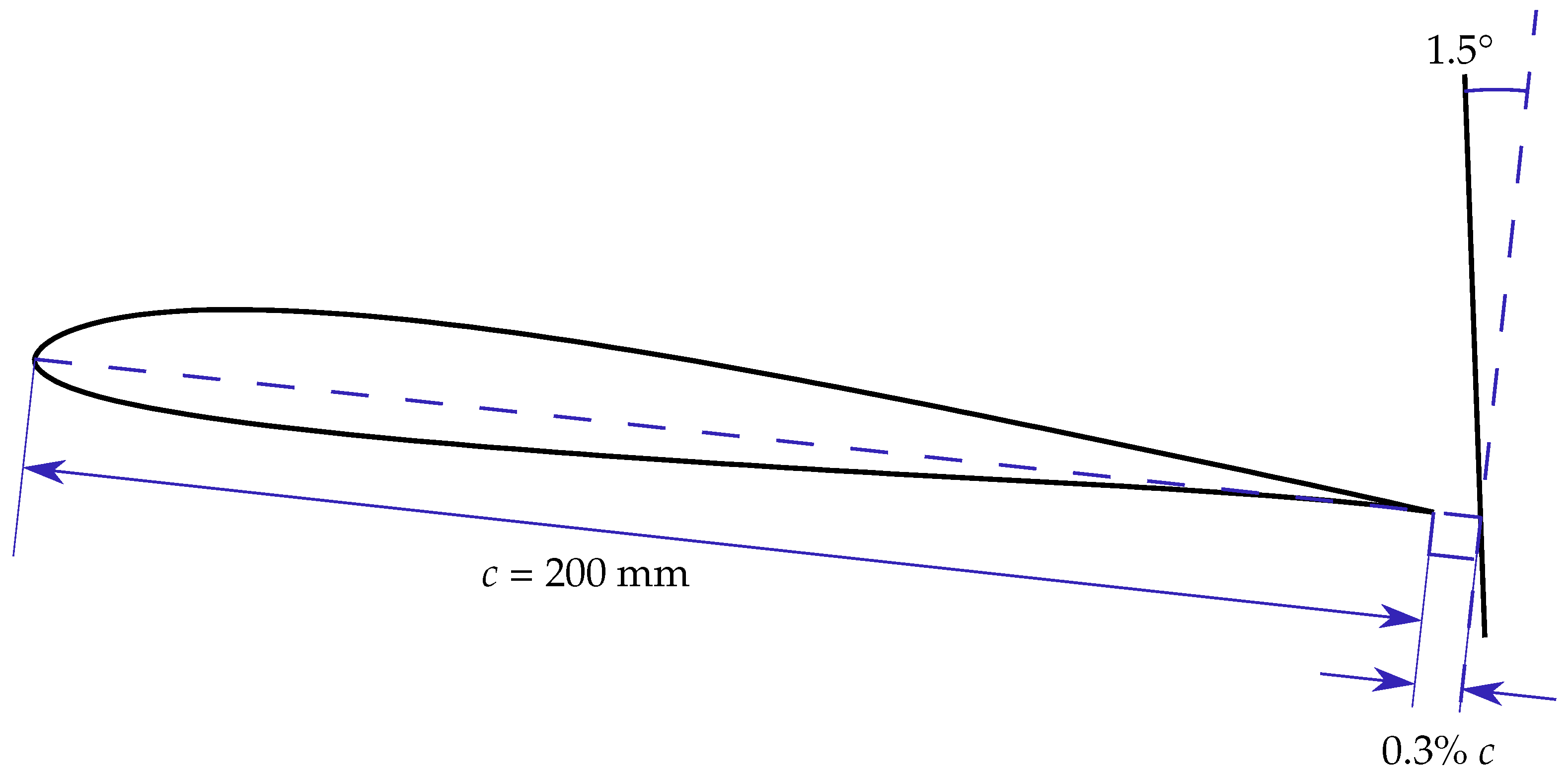
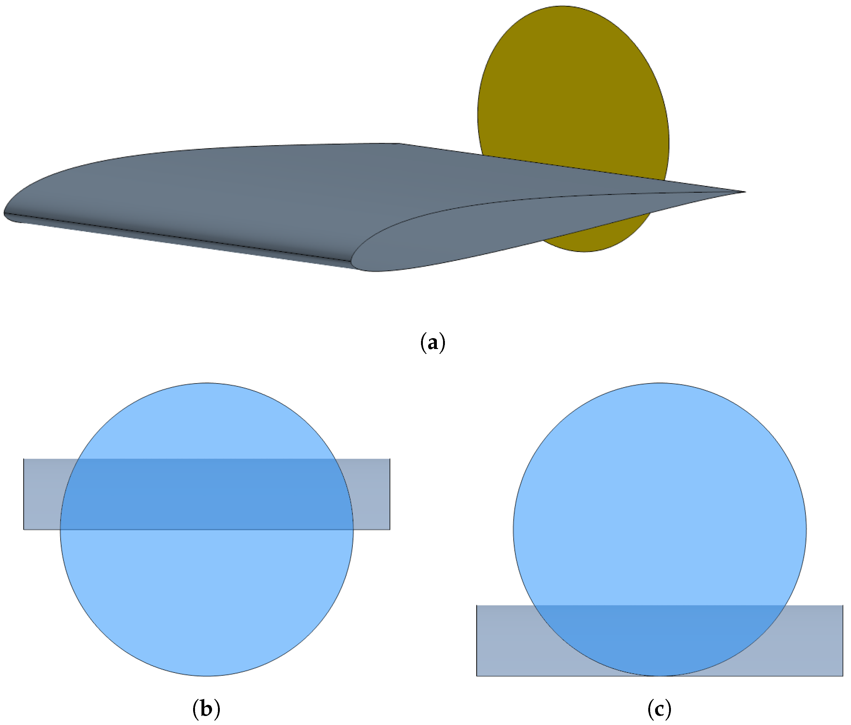
2. Aircraft Description

In this section, the aircraft studied in this work is described. The selection of its different components is the same presented in [24] by Tiseira et al. and [25] by Serrano et al. The aircraft data is shown in Table 1, and Figure 1 shows a schematic view of it.
The study uses data from computational fluid dynamics (CFD) simulations. In order to reduce the computational complexity while still achieving accurate and realistic results, all simulations consist of a 2.5D domain.
The domain consists of a single propeller and a portion of the wing affected by that propeller. In this way, the induced drag of the wing caused by three-dimensional effects is not directly simulated. However, the value of the induced drag is calculated based on the lift of the wing portion and an estimated Oswald factor. The details of the domain regarding measures and boundaries will be explained in the next section.
The choice of these two components was carried out taking into account the mission of the aircraft, which is a fixed-wing, long endurance UAV with an MTOM of 25 k g , driven by several propellers. The aircraft is similar to the Penguin C from UAV Factory [26] and the TARSIS 25 from AERTEC Solutions [27], and has a wing span of 2 m .
For the wing, a single SD7003 airfoil has been used, designed to operate with low parasitic drag at low Reynolds number, which makes it particularly attractive in the application of civil UAVs. This airfoil has been extensively studied in the literature, and high quality experimental and computational data are readily available in multiple references [28,29,30,31].
The propeller chosen for this application was designed by the University of Illinois in Urbana-Champaign. It is the DA4052 model, for which complete geometric data as well as experimental characteristic curves produced in a wind tunnel are found [32]. These data were used to validate the numerical simulations, which were carried out by means of the Blade Element Method [33]. A total of 13 of 80 m m propellers are used for the whole aircraft. The propeller size and the number of propellers were chosen to maximise the specific range of the aircraft, which is the distance flown for each unit of fuel consumption, in a hybrid-electric configuration powered by a four-stroke engine, as described in [24].
In all the simulations, the total thrust generated by the propellers was equal to the total drag of the whole aircraft. For that, the drag was estimated as in Equation (1):
D = 1 2 · ρ · U 2 · S · ( C D , 0 , wing + C D , 0 , extra + C L 2 π · 🜇 · e ) ,
where ρ is the far-field air density, U is the upstream wind speed, S is the wing surface, C D , 0 , wing is the parasitic drag coefficient of the wing and C L is the lift coefficient. C D , 0 , extra , on the other hand, is the parasitic drag of the rest of the aircraft: this includes the fuselage, the empennage, and the landing gear. The values of C L and C D , 0 , wing are directly computed using data from the simulations, whereas C D , 0 , extra is computed using geometrical information of aircraft with a similar mission. This includes the mentioned TARSIS 25 and Penguin C, as well as values from Harmon and Hiserote’s aircraft [10,34]. Finally, the Oswald efficiency factor e is estimated using standard methods as described in [35,36]. The aspect ratio, 🜇, is set to 10.

3. Methods

In this section, the computational methods are presented. This includes the CFD setup, the way a wing section is simulated and the method for performing the modal decomposition of the friction and pressure coefficients.

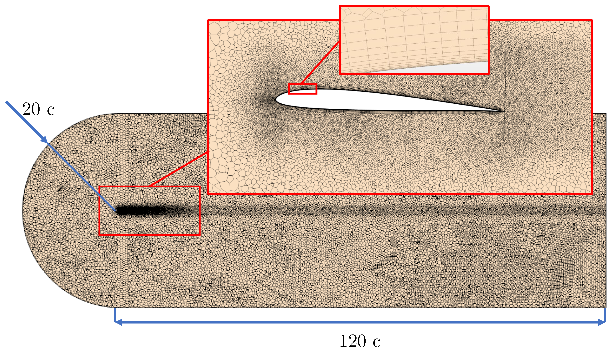
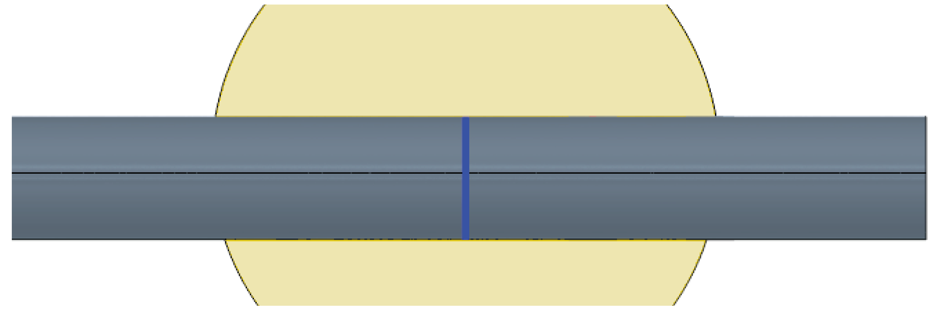
3.1. Computational Domain

All the case studies follow the same computational setup shown in [24,25]. In both cases, 2.5D simulations of a wing section were performed, and the size of the domain was proven to be big enough so the position of the far field boundary conditions did not affect the final solution. The upstream boundary condition is located 20 chords from the wing and uses a free-stream speed condition. Downstream of the wing, a pressure outlet boundary condition is set. The lateral boundaries are set as symmetry boundary conditions. Finally, the surface of the wing is modelled as a non-slip, smooth wall. A sketch of the computational grid is shown in Figure 2.
In all the simulations, the propeller is located over the trailing edge of the wing section, but different positions are studied. The propeller is, in any case, modelled with a single virtual disc actuator, using the Blade Element Momentum Theory (BEMT). This 80 m m of diameter propeller is separated from the trailing edge around 1 m m in the direction of the chord. The relative angle between the profile and the normal to the propeller, the draft angle, is set at 1.5°. These dimensions are shown in Figure 3, and have been chosen based on previous studies [24,25].
The main geometric aspect that varies between cases is the vertical height of the actuator disc. This height, measured as the distance between the propeller shaft and the trailing edge, is expressed as a fraction of the propeller radius. This way, 0% represents that the center of the propeller is aligned with the trailing edge, whereas at the other extreme, at 100%, the entire propeller is above the trailing edge. The latter conditions represent the case with the minimum influence over the pressure side of the wing, whereas the former produce the maximum level of boundary layer ingestion. These two positions are represented in Figure 4, below a sketch of the wing section where the propeller disc is visible.

3.2. CFD Methodology

The CFD simulations are carried out in the same way as described in [24,25], using the proprietary software Simcenter STAR-CCM+ with a finite-volume, steady-state, Reynolds-Averaged Navier–Stokes (RANS) equation approach. As the flow speed is relatively small in all the simulated cases, the flow is modelled as incompressible. A Spalart–Allmaras model is chosen to compute the Reynolds stress tensor.
The domain is meshed with a polyhedral mesh except for the boundary layer around the wing: in this zone, a 14-layer prismatic mesh with a geometric grow distribution is applied in a total thickness of 3 m m , which is of the order of the displacement thickness of the boundary layer. This boundary layer mesh ensures a non-dimensional distance from the wall to the first cell centroid y+ less than one in 99% of the wall around the airfoil. Keeping a value of y+ lower than 1 is a requisite of the model to solve the viscous sublayer of the boundary layer without using wall functions. Finally, the mesh size of the polyhedral mesh near the walls has been kept at 1 m m . This mesh size was set after performing a mesh independence study in which the discretisation error was computed by means of a Richardson extrapolation, as seen in [24].
Five different propeller positions were simulated over the trailing edge, between 0% and 100%. For each position, nine angles of attack between 1° and 9° and three different Reynolds: 3 × 10⁵, 5 × 10⁵ and 7 × 10⁵. These Reynolds number correspond to a wind speed at sea level and 15 °C of 22.0 m s−1, 36.7 m s−1 and 51.4 m s−1.
The propeller, modelled with a BEMT actuator disc, uses geometrical data and airfoil drag polar results obtained from a panel method with interactive boundary layer corrections code, XFLR5 [37], which is based on Mark Drela’s XFOIL [38]. The rotational speed of the propeller was set so that the total thrust produced by all the propellers was equal to the total drag of the aircraft in each simulation, as shown in Equation (2).
T · n propellers = D = 1 2 · ρ · U 2 · S · ( C D , 0 , wing + C D , 0 , extra + C L 2 π · 🜇 · e ) .
The simulations of both the airfoil and the propeller, separately, were validated against experimental and high-fidelity simulations found in the literature.

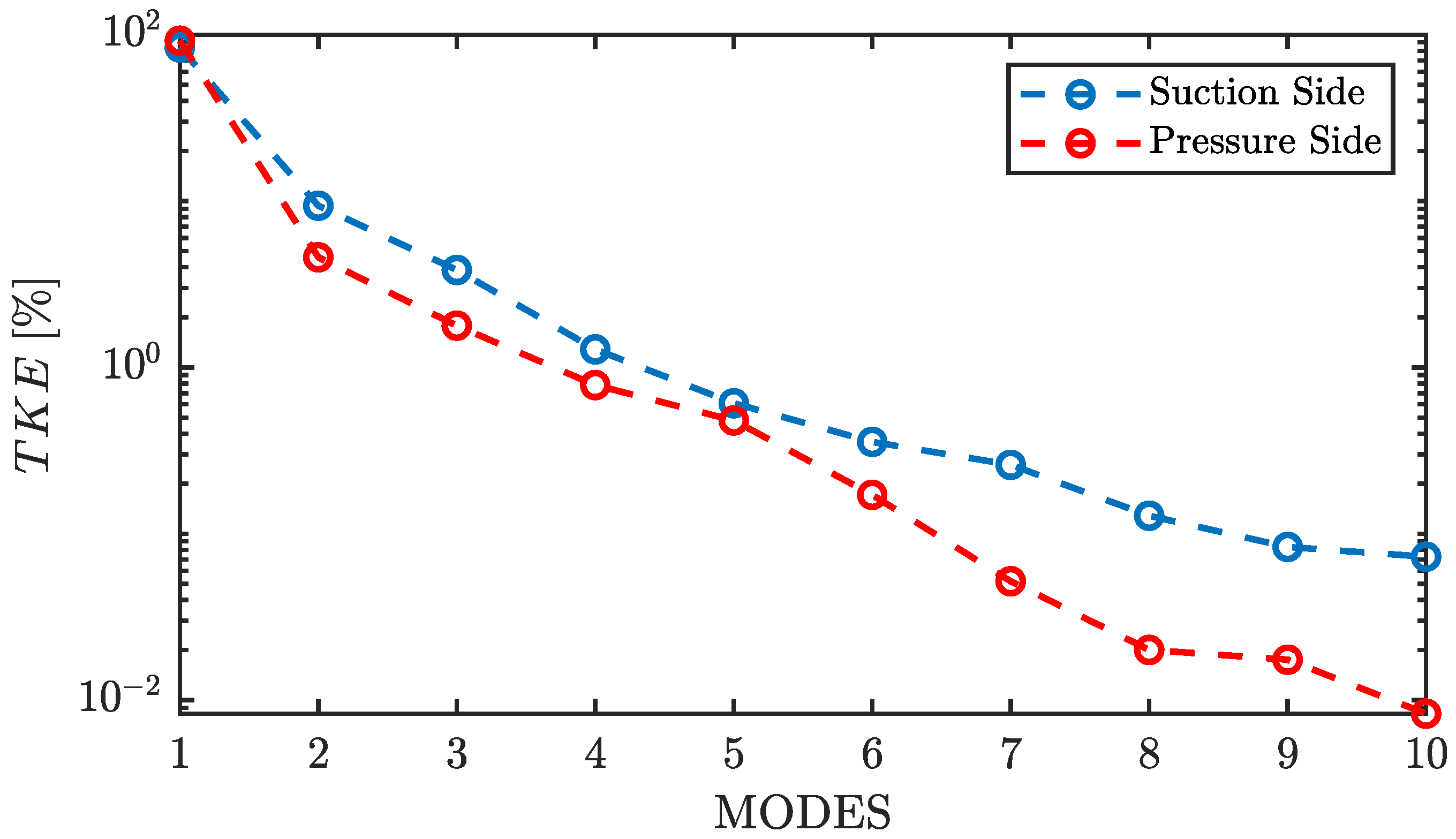
3.3. POD Application

Once all the simulations were carried out, the pressure coefficient C p and the friction coefficient C f were extracted at each simulation. The coefficients were extracted by using a single plane, which divides the actuator disc in half just in the middle of the domain Figure 5. For a fixed Reynolds, each coefficient distribution is a function of the angle of attack α and the relative height of the actuator disc above the wing h.
As the process for working with one or the other coefficient is analogous, from now on the equations are written based on the pressure coefficient.
In each simulation, 300 spatial points over the wing surface were taken, and since five positions and nine angles of attack are simulated, 45 different distributions were generated. The combination of these data yields a working matrix of 45 × 300 elements, U. Each row corresponds to the coefficient distribution over the airfoil for one combination of angle of attack and propeller position.
Once the matrix was obtained, the coefficient was decomposed into a summation of a series of deterministic spatial functions, also known as spatial modes, ( ϕ k ) that depend only on the point of the airfoil where said aerodynamic coefficient is studied. The series is expressed in Equation (3) for the pressure coefficient as a function of the chord position x, the angle of attack α and the relative propeller position h, which is the propeller shaft height over the trailing edge divided by the propeller radius.
C p ( x , α , h ) = k = 1 a k ( α , h ) ϕ k ( x ) .
The modes are in turn modulated by what are known as configuration coefficients ( a k ) that depend on the 45 configurations described in the problem.
Once the matrix U was obtained, it was possible to calculate its covariance matrix C, an indication of the degree of correlation of the data, as expressed in Equation (4).
C = 1 m 1 U T U ,
where m is equal to the total amount of distributions, 45.
After obtaining the covariance matrix, its eigenvalues and eigenvectors were computed, which were then sorted from the largest eigenvalue to the smallest. A set of 300 λ eigenvalues was obtained, as well as 300 eigenvectors. The eigenvalues were arranged in a diagonal matrix Λ, whereas the eigenvectors were arranged as columns in a matrix Φ. The relationship between C , Φ and Λ is expressed in Equation (5):
C = Φ Λ Φ 1 .
By ordering the eigenvalues, it was possible to determine the percentage of the energy content, TKE , which explains each mode, as shown in Equation (6). In this way it was possible to assess how many modes explain most of the aerodynamic behaviour of the coefficients.
TKE j = λ j j = 1 300 λ j .
Once the modes were obtained, the configuration coefficients that model the modes were computed through the matrix A expressed in Equation (7), where the original dataset U was projected onto each n mode.
A = U Φ = a 11 a 1 n a 21 a 2 n a m 1 a m n .
In A , each coefficient a i j is the result of projecting the data measured on the airfoil in configuration i over mode j. Thus, each column of matrix A had the configuration coefficients for each of the 45 configurations. Each configuration i corresponds to a combination of propeller position and angle of attack.
Since it is possible to reconstruct the original matrix U through the sum of the contributions of its modes multiplied by the configuration coefficients, it is possible to rewrite U as the sum of the effect of each mode as in Equation (8):
U = A Φ 1 = k = 1 n U ˜ k = k = 1 n u ˜ 11 k u ˜ 1 n k u ˜ 21 k u ˜ 2 n k u ˜ m 1 k u ˜ m n k = k = 1 n a 1 k a 2 k a m k ϕ 1 k ϕ n k .
Therefore, if instead of adding all the modes, only those that represent the most TKE of the system are chosen, it is possible to compare the original signal with that reconstructed with a few modes.

4. Results and Discussion

This section presents the different results of the study. It is divided into four parts: the first one, in which the results of the modal decomposition of the pressure coefficient is presented; the second one, in which the same is done for the friction coefficient; a third one, where, using the modal decomposition of the pressure and friction coefficients, the lift and drag coefficients are reconstructed; finally, a subsection in which the pressure and friction coefficients of non calculated cases are computed using a surrogate model.

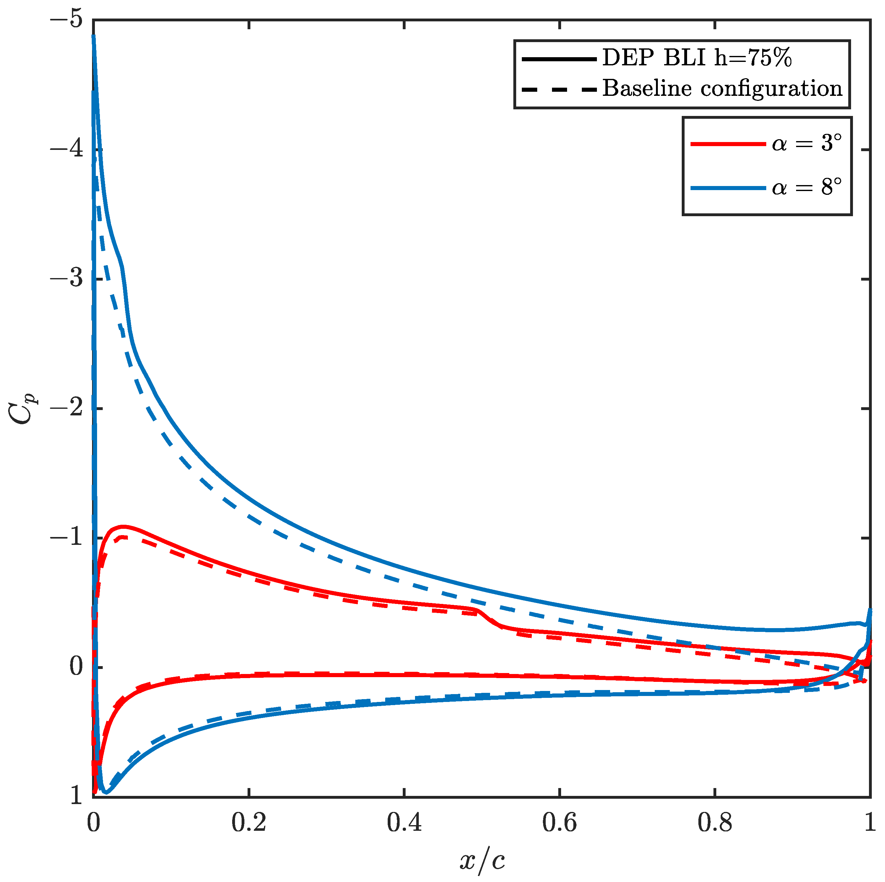
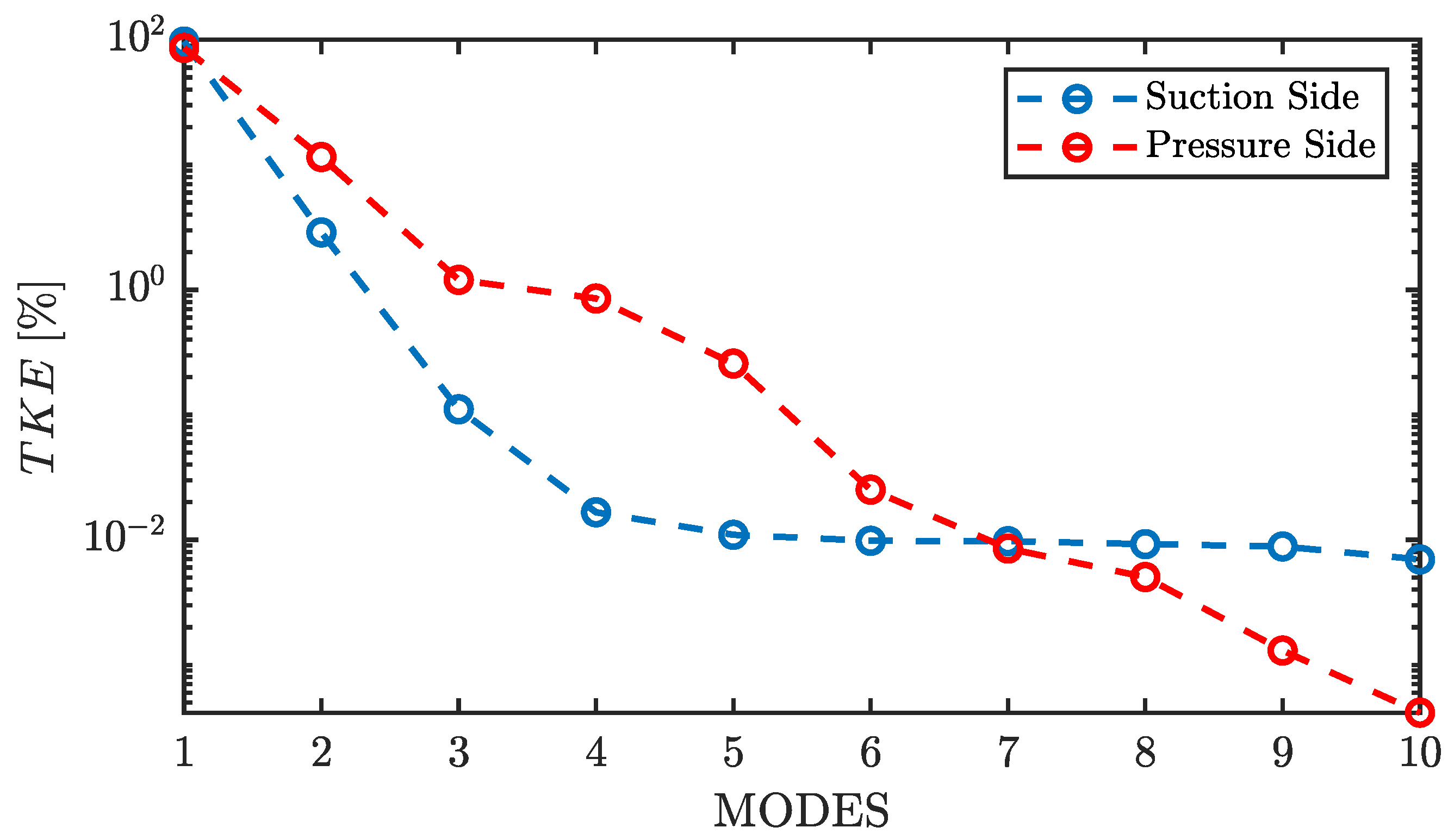
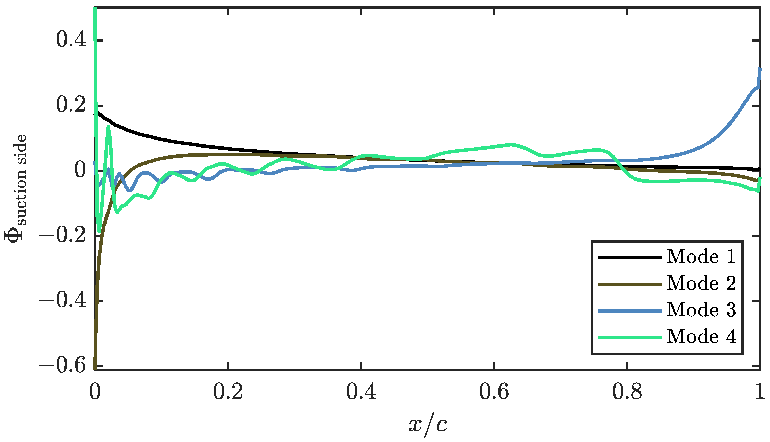
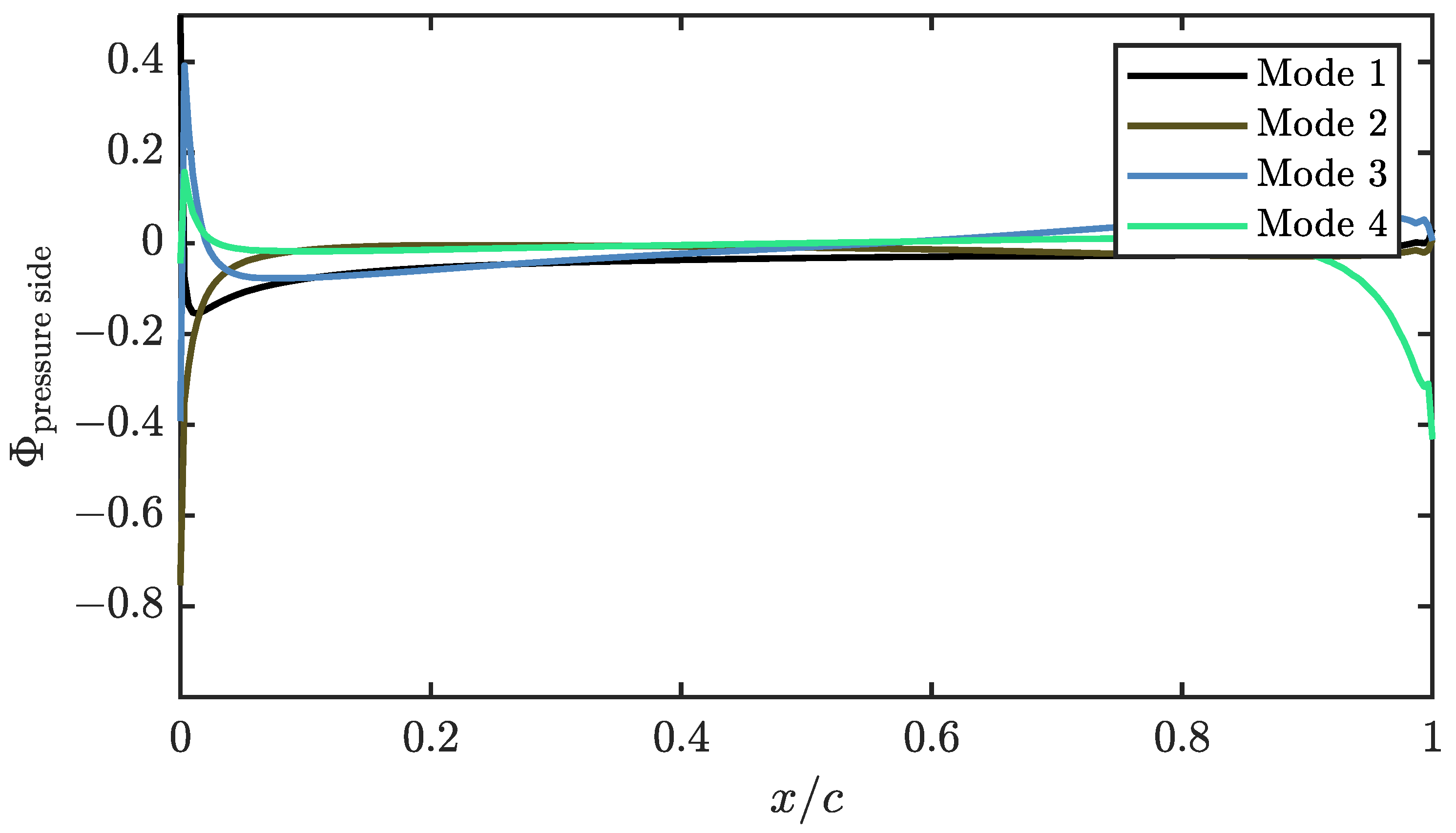
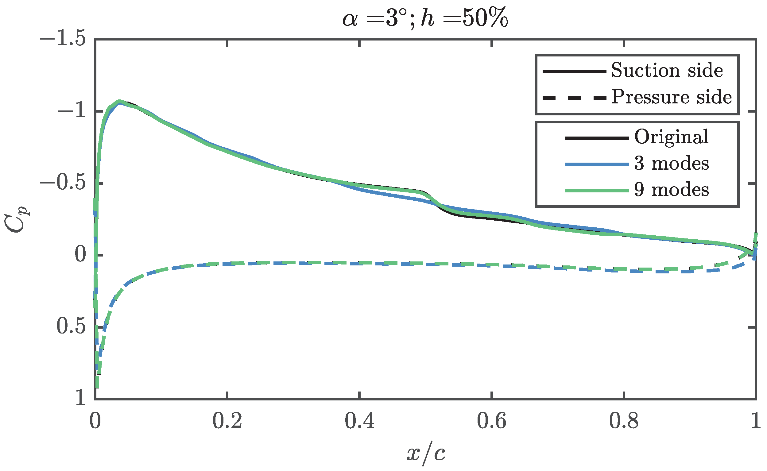
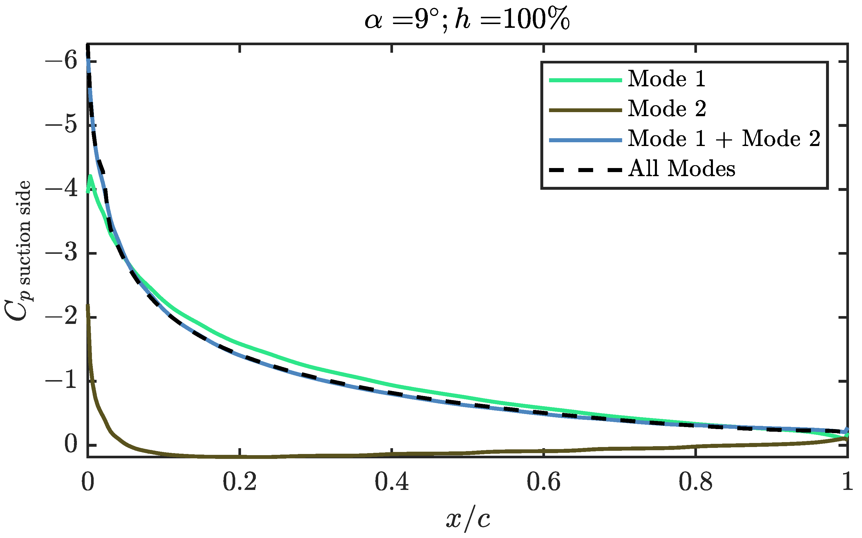
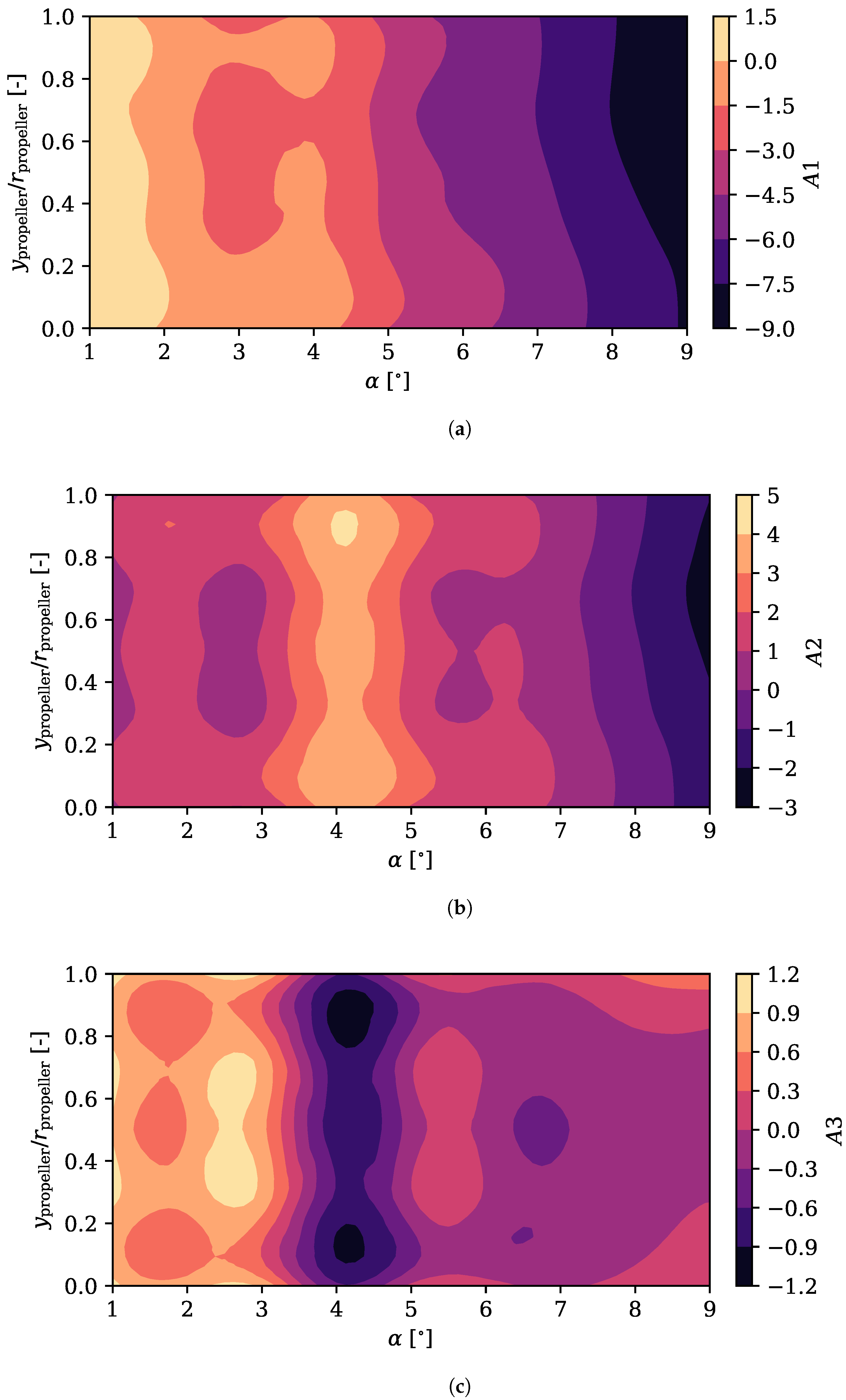
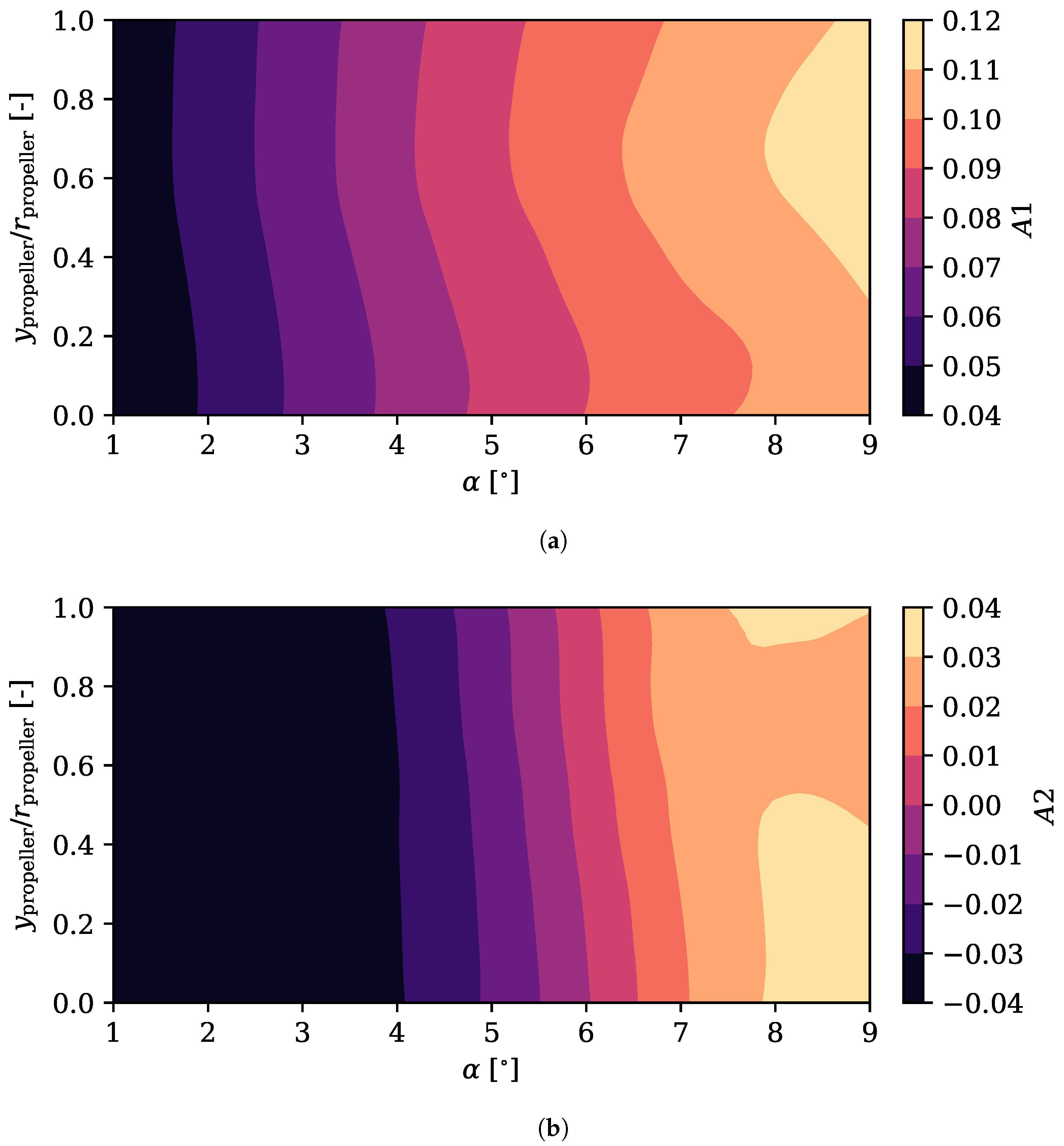
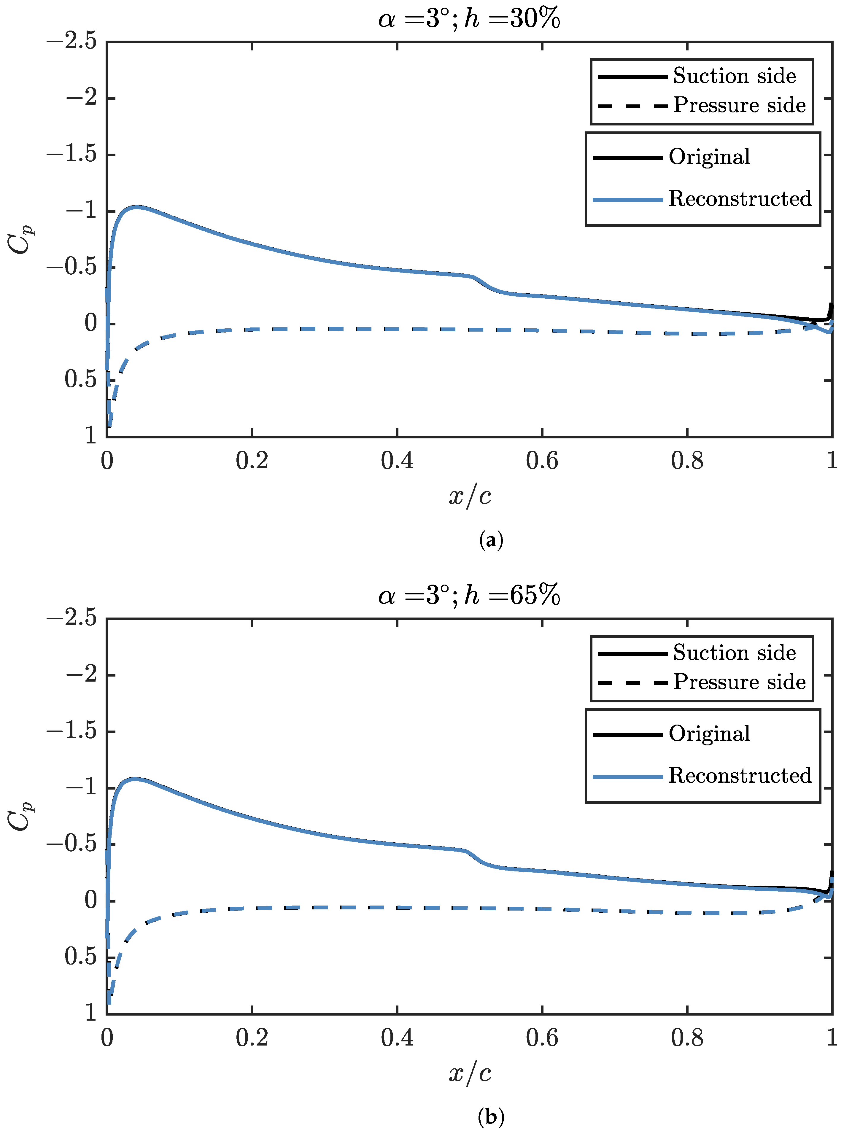
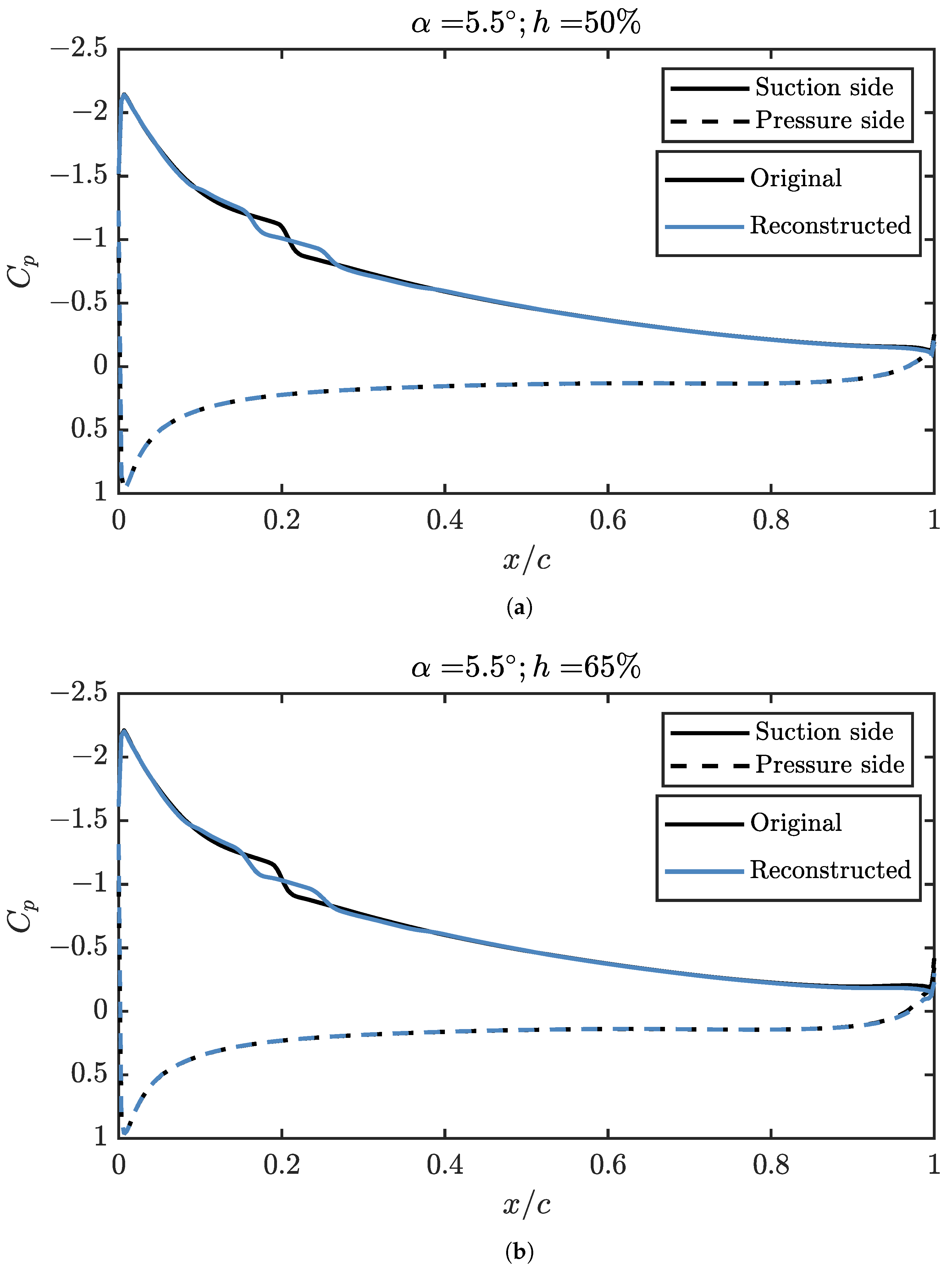
4.1. Pressure Coefficient Analysis Using POD

As it was drawn as a conclusion in [25], the pressure coefficient is influenced by the position of the propeller over the trailing edge, giving rise to higher suction peaks in the case of higher positions. Furthermore, it is possible to observe that the laminar separation bubble (LSB) occurs closer to the leading edge at higher propeller positions since the influence of the propeller height translates into a change of the circulation around the airfoil, similar to flying at a highest apparent angle of attack.
The C p is also highly modified depending on the angle of attack, as shown in Figure 6. For a fixed propeller position, the suction peak grows on the suction side or extrados as the angle of attack α increases, contributing positively to the lift of the airfoil. From the suction peak, the flow over the extrados encounters an adverse pressure gradient that decelerates the flow. This sudden increase in pressure leads to instabilities in the laminar boundary layer and causes the LSB to occur near the leading edge so that the higher the angle of attack, the further upstream the bubble is. Regarding the pressure side, when increasing the angle of attack, an overpressure is produced that also contributes, although to a lesser extent, to the lift of the wing. As expected, the behaviour corresponds to what can be observed over an airfoil without BLI, although the actual magnitude and distribution of the pressure coefficient is modified.
Figure 6 exemplifies in solid lines for a propeller height position of 75% the change in the C p of the suction side (mostly negative values of C p ) and pressure side (mostly positive values of C p ) due to the increase in the angle of attack, along the normalised chord of the airfoil. As a reference, and in dashed lines, the results for a case without BLI is also shown.
As mentioned in the previous section, it is possible to know the main effects of the height of the propeller over the trailing edge and the angle of attack affect the C p through the percentage of TKE that their modes explain. To make the analysis more conclusive, the pressure coefficient of both the intrados and extrados are studied separately: in this way, different number of modes can be used to recreate the C p of each part.
Figure 7 shows the percentage of TKE explained by the first 10 TKE modes, in red for the pressure side and blue for the suction side.
Since the modes have been ordered as a function of higher to lower eigenvalue, the first modes are those that explain the most energy of the problem. In the case of the suction side, 96% of the energy is explained through the first mode, and 3% is explained by the second, with the contribution of the following modes being marginal. In the pressure side, the first mode explains a lower percentage of energy compared to the suction side, 86%, but it is still much higher than the rest of the modes, whereas the second explains 12% of TKE .
In Figure 8 and Figure 9, the first four spatial modes of the C p of the suction side and the pressure side are represented, respectively. In the extrados, both the first and second modes have a homogeneous shape compared to the lower energy modes. These modes have an important weight in resolving the pressure coefficient near the suction peak, while less energetic modes have a greater influence on the explanation of the pressure behaviour near the trailing edge. In the case of the pressure side, the modes behave in a similar way to the suction side. However, it can be seen that the first three modes provide most information near the leading edge, with the fourth mode being the one with the greatest weight near the trailing edge.
Although the first three modes of the suction side explain 99.5% of the TKE , they are not enough to explain the transitional bubble over the airfoil, as can be seen in Figure 10. In this figure, the angle of attack is set to 3° and the relative height of the propeller to 50%. It can be seen that, while the suction peak, which concentrates the largest fraction of TKE in the problem, is well defined, from 50% of the chord it is possible to find discrepancies. A greater number of modes are required if the aerodynamic behaviour is to be modelled more realistically. The first three modes are enough to reproduce a shape similar to that of a LSB, albeit with a lower intensity and a different position, moved towards the trailing edge. Regarding the trailing edge behaviour, it is relatively well reproduced in any case, even when only three modes are used to reconstruct the solution. As expected from the results of Figure 7, a reduced number of modes is enough to get most of the behaviour of the pressure coefficient distribution, so the lift coefficient, pitching moment and structural stresses over the skin can be computed with good accuracy from a limited amount of information. Only when detailed information is required, as it is for the position of the LSB, more than three modes are necessary.
It is possible to obtain more information about the modes by representing the configuration coefficient that modulate them. Figure 11 represents the configuration coefficients of the first 2 modes of the C p of the extrados as a function of the relative height of the propeller and the angle of attack.
The first configuration coefficient, A 1 , varies slightly with the height of the propeller for a given angle of attack. From another point of view, for a given relative height, this coefficient is is much more variable with the variation of the angle of attack. The value of the coefficient A 1 has a negative value for any combination of height and angle of attack, so it influences the mode in all positions, finding the greatest influence at the maximum angle of attack and close to the highest position. At around 75% of relative propeller height, however, the trend is inverted and the value of A 1 starts to decrease: the propeller is too high and the effects of the boundary layer ingestion are reduced.
This position is represented in Figure 12, where it can be seen that the first mode practically explains all the C p by itself. Rising the propeller position can be used to produce higher lift: for a given angle of attack, the value of the C p due to the first mode can be increased 10% to 20% by rising the propeller to around 75% while maintaining the thrust equal to the drag.
The configuration coefficient of the second mode, A 2 , have a similar behaviour to the first, that is, it is possible to observe a greater variation with the angle of attack than with the propeller height. However, the coefficient values are far from the first. In this case, the absolute maximum values are lower, which makes sense since this mode explains less energy. Furthermore, the value of the coefficient goes from negative to positive when increasing the angle of attack, reaching a null value for α around 6° to 7°. The variation with the angle of attack seems to be more nonlinear than in the case of the first mode, and makes the suction peak narrower and more intense as α increases. The same can be said for the position of the propeller: as it moves up, the configuration coefficient increases, what moves the suction peak towards the leading edge, makes it narrower and more intense. The shift due to changes in the propeller position is bigger at a height around 50%. This may be explained by the fact that, at lower positions, the propeller affects too much the pressure side of the airfoil, whereas at higher positions the amount of ingested boundary layer is decreased.
The same coefficients are presented in the case of the C p of the pressure side Figure 13, including in this case the third coefficient.
The first mode of the intrados has a structure similar to that seen in the first mode of the extrados represented in Figure 11. The trend with the angle of attack and the propeller height is similar, although more nonlinear.
The second and third modes ( A 2 and A 3 ) have more complex structures and explain more TKE than in the case of the suction side, although their effect over the global aerodynamic coefficients is somewhat limited as the absolute value of the C p over the pressure side is smaller. It is interesting to note the peak in value around an angle of attack of 4°. At that position, they maximise the value of C p at the leading stagnation point, widening it. At angles of attack smaller or bigger, the bigger value of the configuration coefficient of the third mode makes the stagnation zone narrower. Regarding the propeller position, at low positions the flow accelerates more over the intrados, reducing the pressure coefficient.

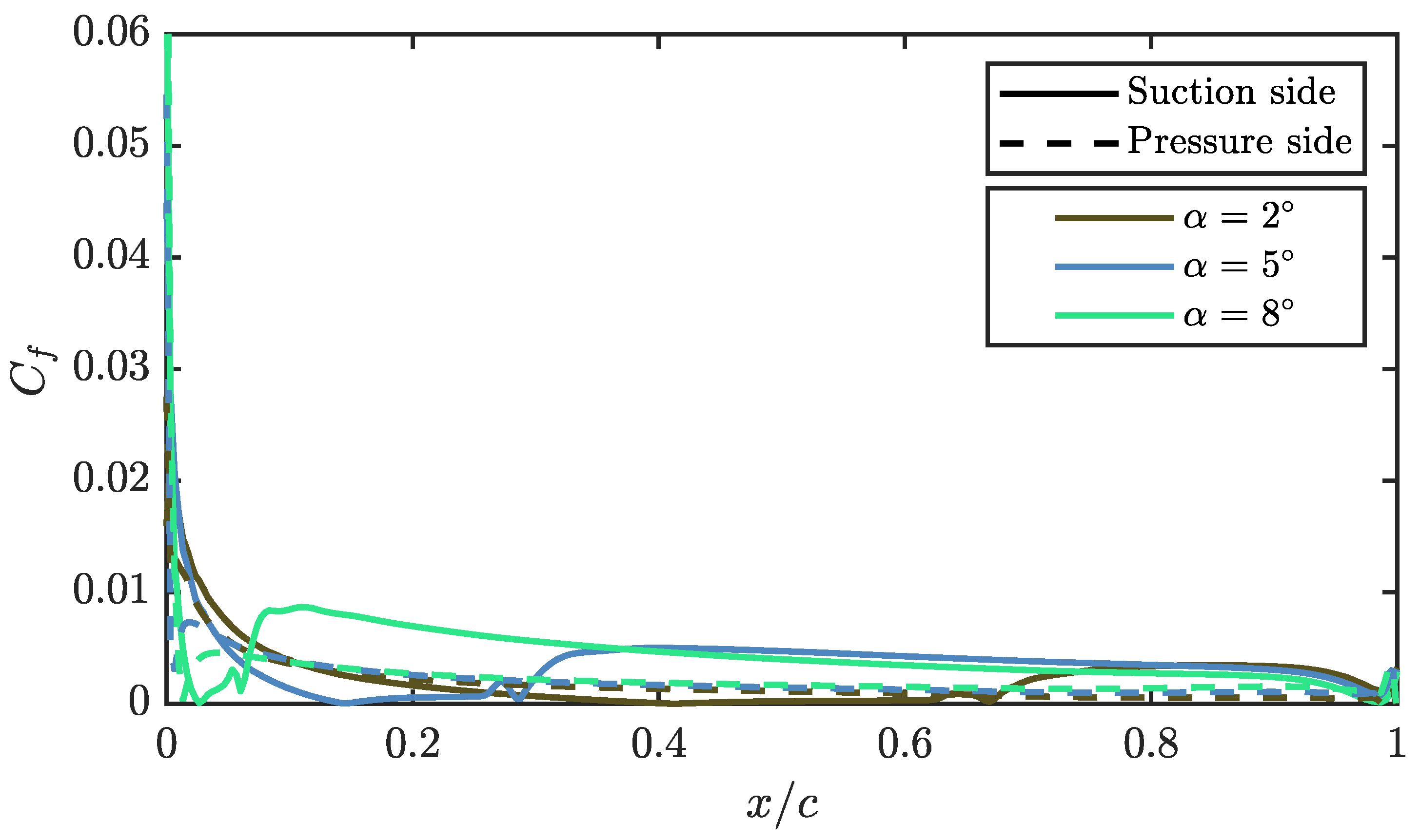
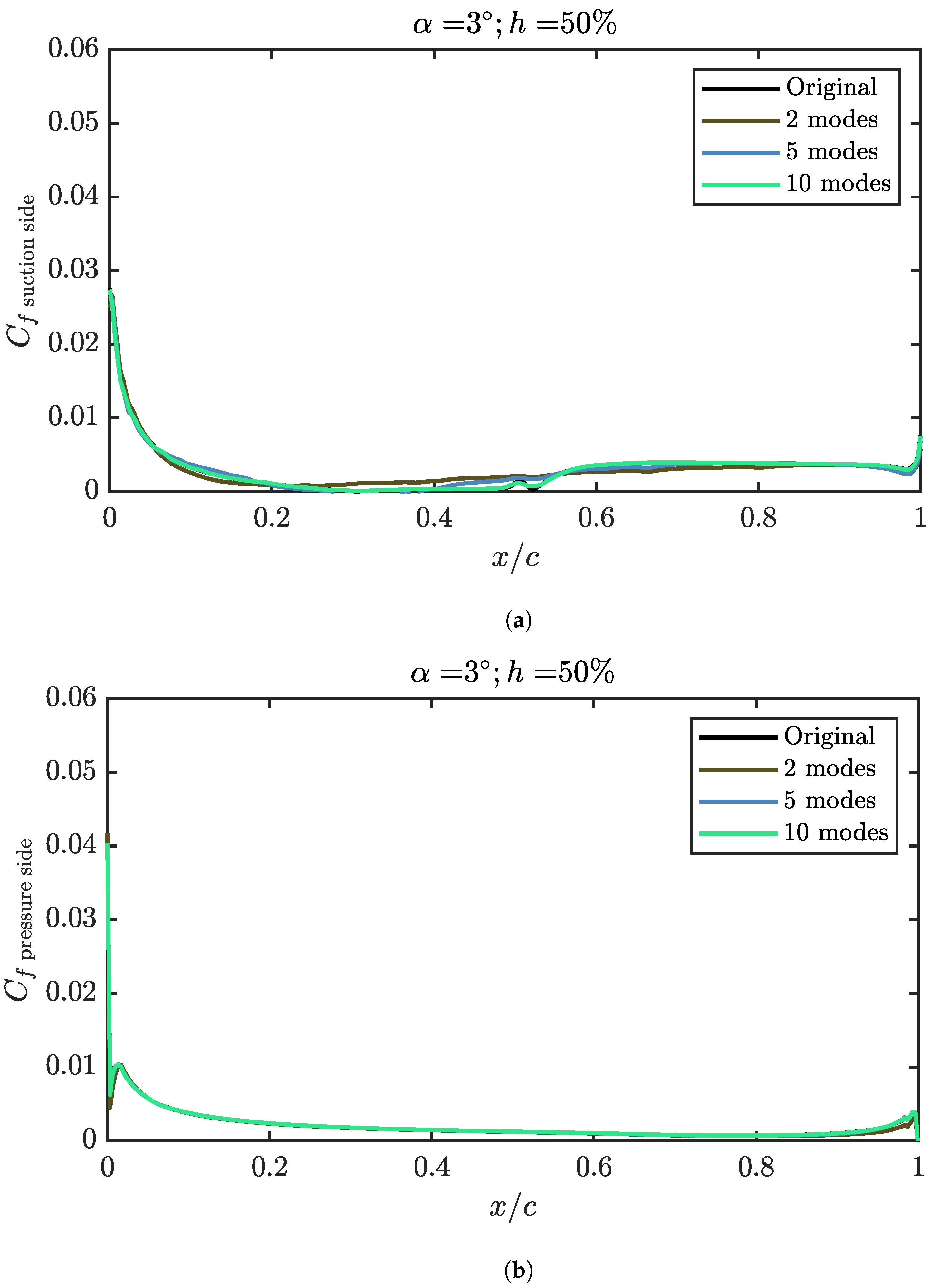
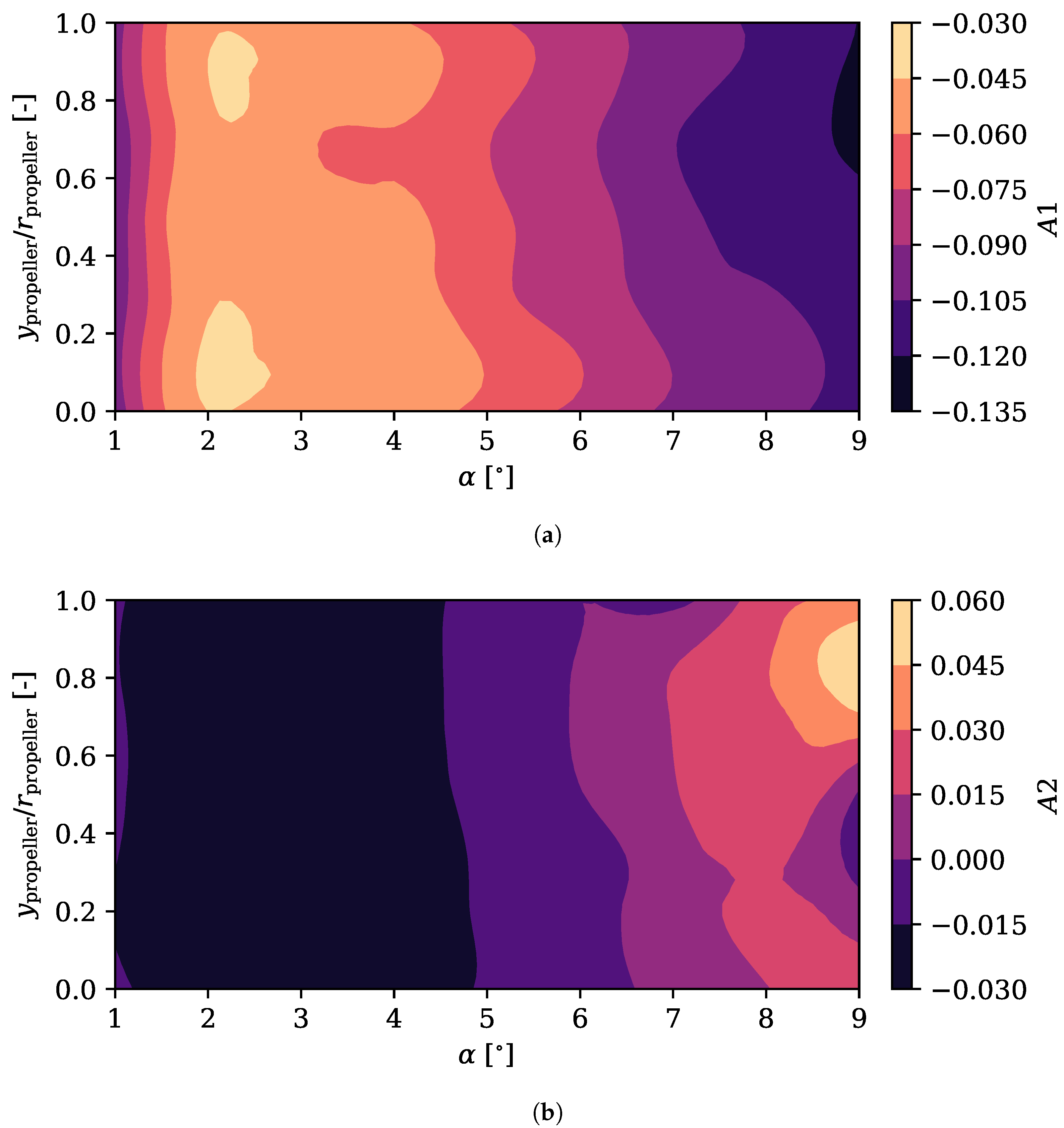
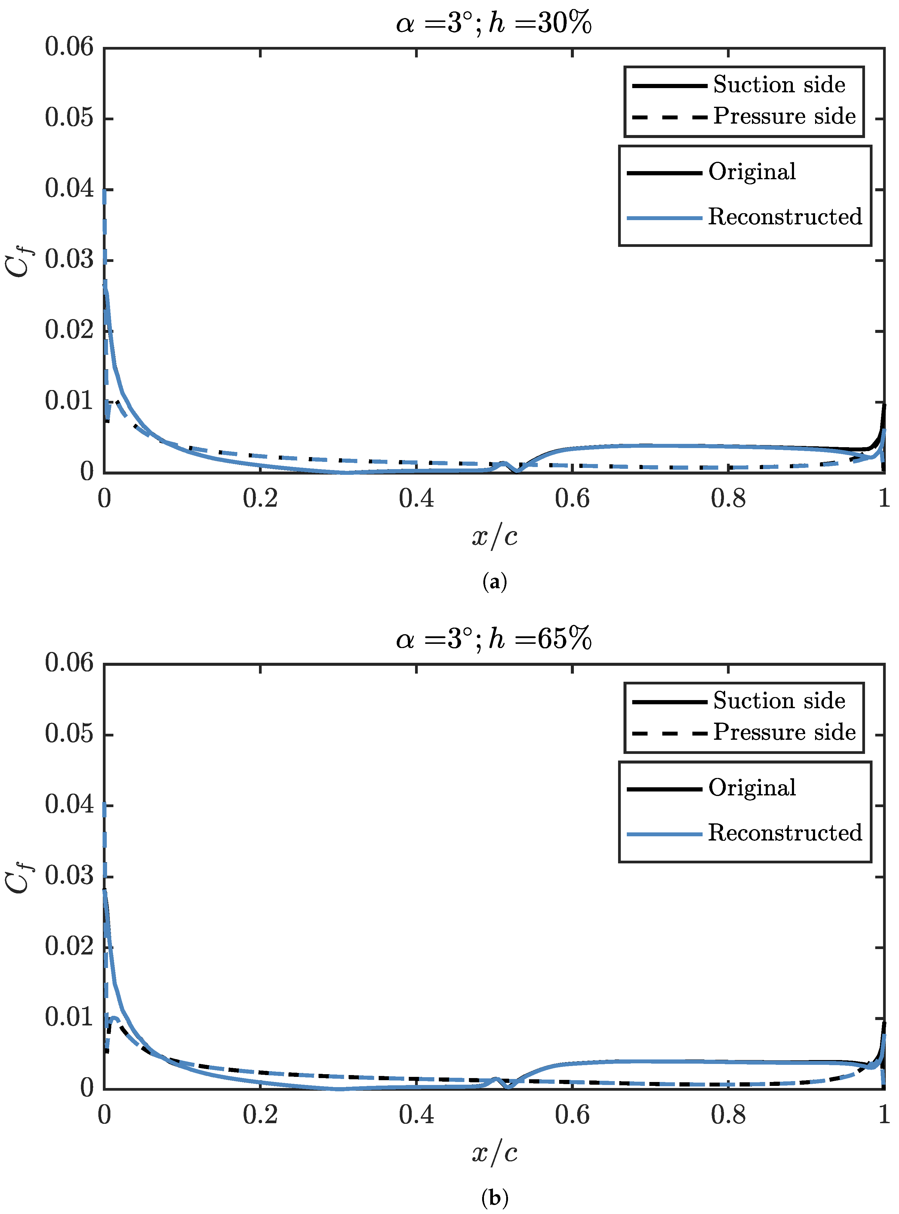
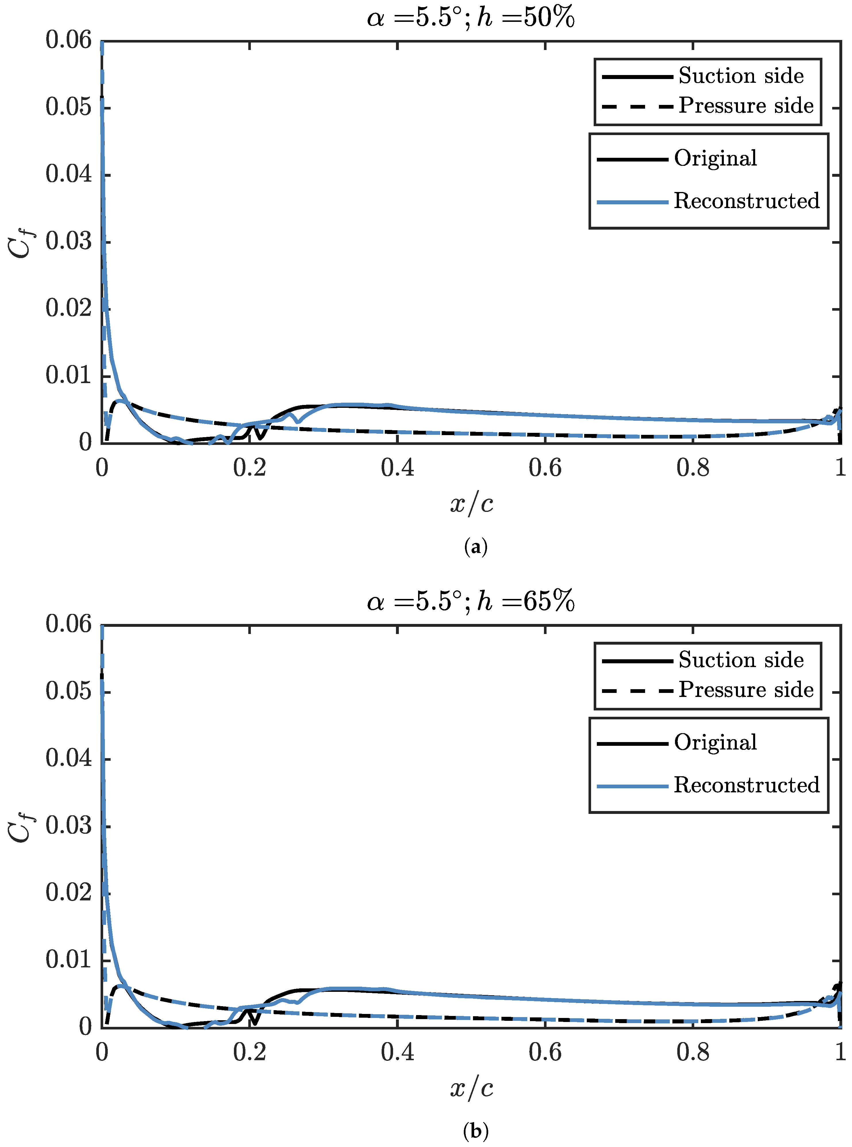
4.2. Friction Coefficient Analysis Using POD

The friction coefficient is studied in the same way as C p . Representing the evolution of this coefficient for a given propeller position 50% on Figure 14, the advancement of the LSB can be observed, marked by the fast growth of C f followed by a null value of the coefficient, indicating where the bubble is located. In turn, the changes in the intrados are small, and the value of C f is practically constant throughout the chord.
The first modes represented in Figure 15 are those that have the most energy and explain the problem in a more significant percentage, both in the extrados and the intrados.
In this case, for the extrados, the energy of the first mode is below 83%, which means that it is necessary to use more modes to accurately represent the problem since they will be more energetic. This can be easily verified in Figure 16a. Even with five modes, there are important differences between the reconstruction and the actual friction coefficient. In order to take into account the behaviour of the transitional LSB, up to ten modes are needed. In the intrados, the C f has a much more homogeneous shape since the LSB does not appear, therefore fewer modes are required for the reconstruction of this side. Indeed, with only two modes, the error reconstructing the friction coefficient over the pressure side is negligible, as it is shown in Figure 16b.
As was done with the C p , it is possible to represent the configuration coefficients of the modes in order to obtain more information. In Figure 17 the two first modes of the extrados C f are represented.
The trend of the first coefficient mirrors the one already seen in the case of C p , getting higher values as the angle of attack increases. Again, a greater variation of the coefficient is observed with the angle of attack than with the height of the propeller. However, in this case, for the highest angles of attack, from 6° onward, the height of the propeller varies to a greater extent the value of the coefficient, obtaining bigger values in the higher positions. This fits with what was stated in [25], where it could be observed that by increasing the relative position of the propeller on the trailing edge, the friction coefficient of the suction side increased, increasing the parasitic drag. Most of the effect can be explained by the first mode alone, which does not carry enough information to resolve the transitional separation bubble: it is expected that the parasitic drag of the wing due to the skin friction over its suction side could be accurately interpolated to other non-simulated conditions even if the LSB is not well resolved. For the second mode, the effect of the propeller position is more limited.
Looking at the configuration coefficients of the pressure side in Figure 18, it is possible to observe that the behaviour of the first coefficient is similar to that of the suction side but with an inverted value. The value of the coefficient decreases as the angle of attack decreases, reaching the minimum at the highest angle of attack and at the highest positions. This behaviour is due to the fact that in the higher positions, a small percentage of the actuator disc influences the pressure side, reaccelerating the flow to a lesser extent and giving rise to a smaller C f . The parasitic drag due to the friction coefficient over the pressure side of the wing should be more accurately interpolated in this case, as there is no transitional bubble that produces more TKE for higher modes.

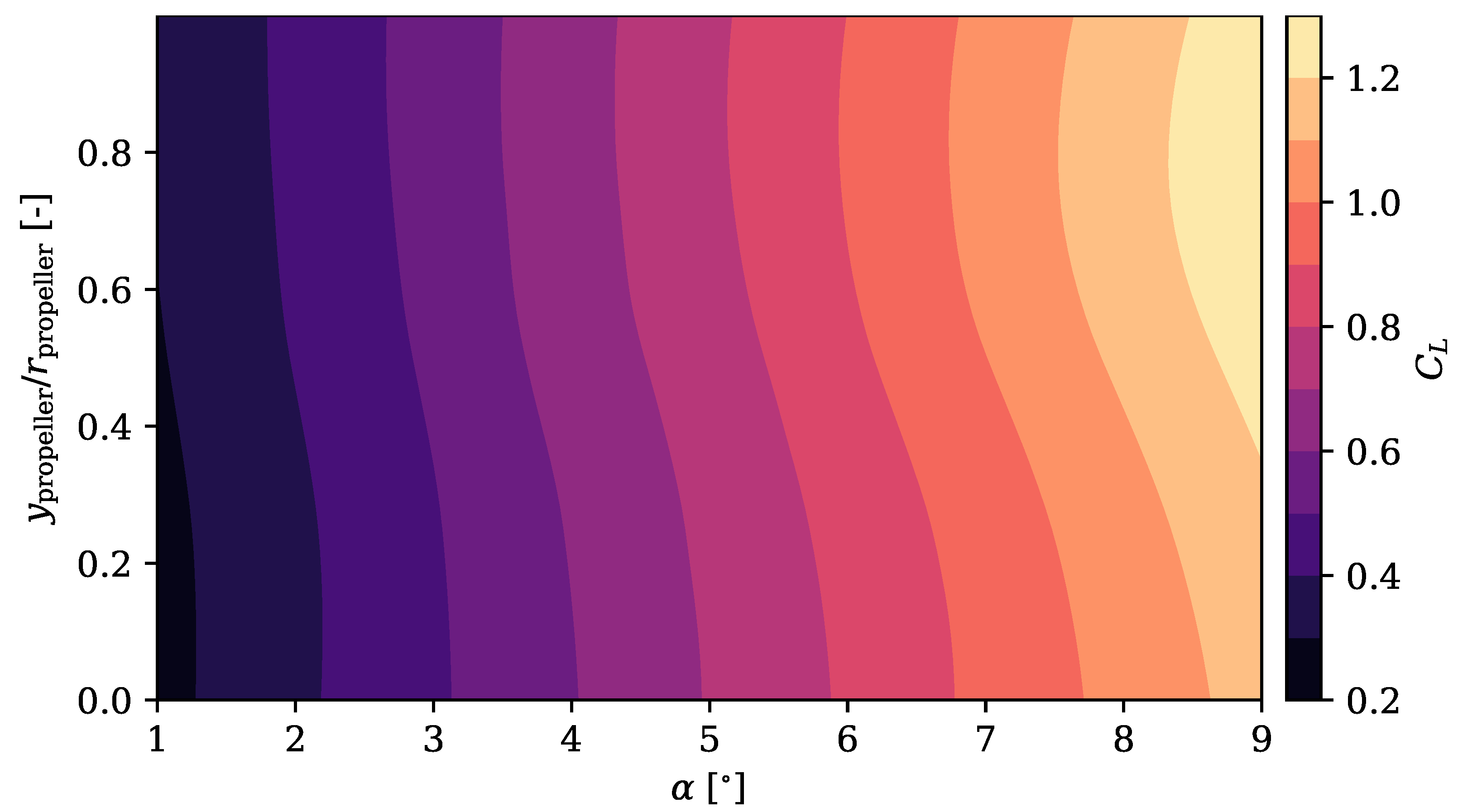
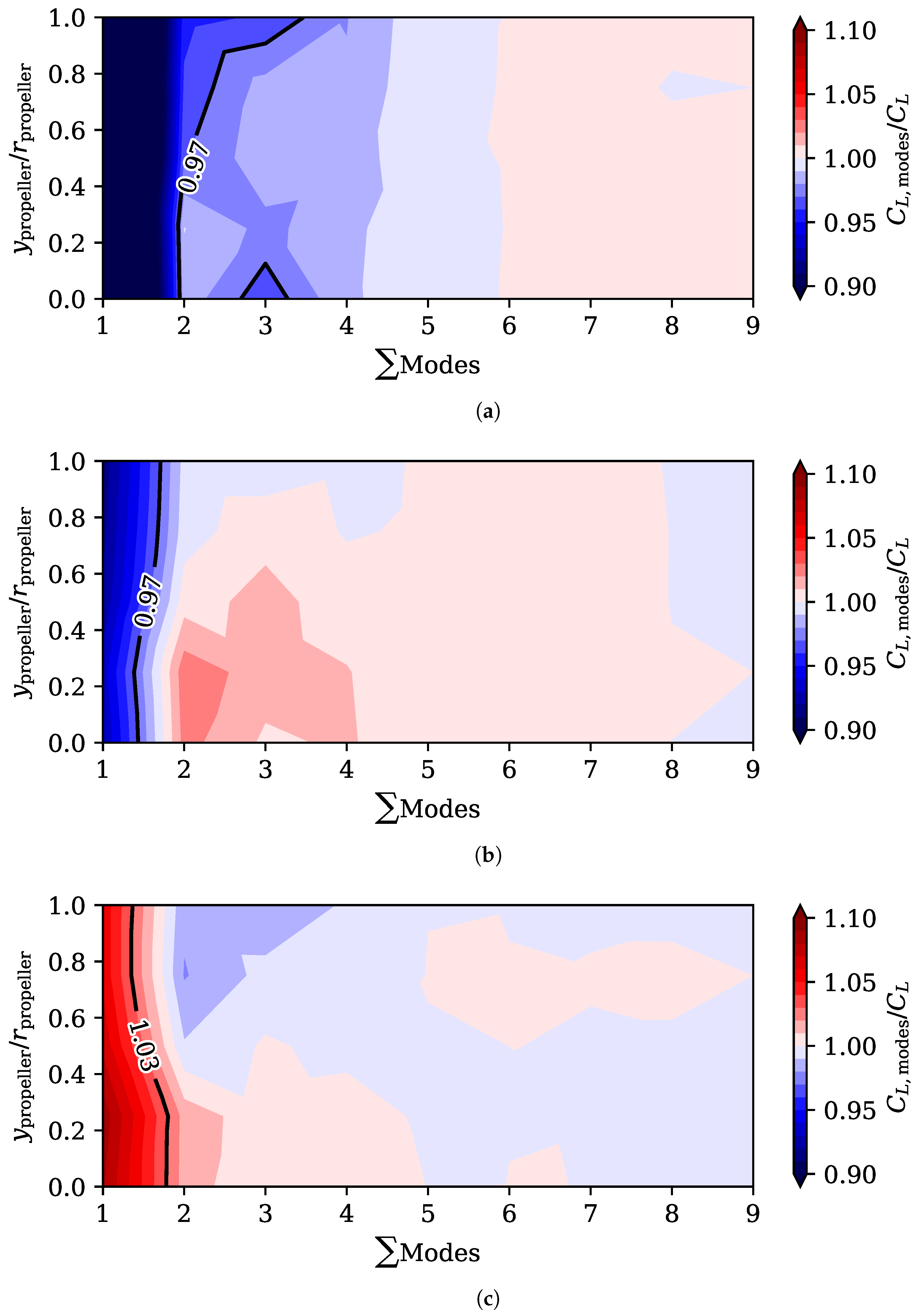
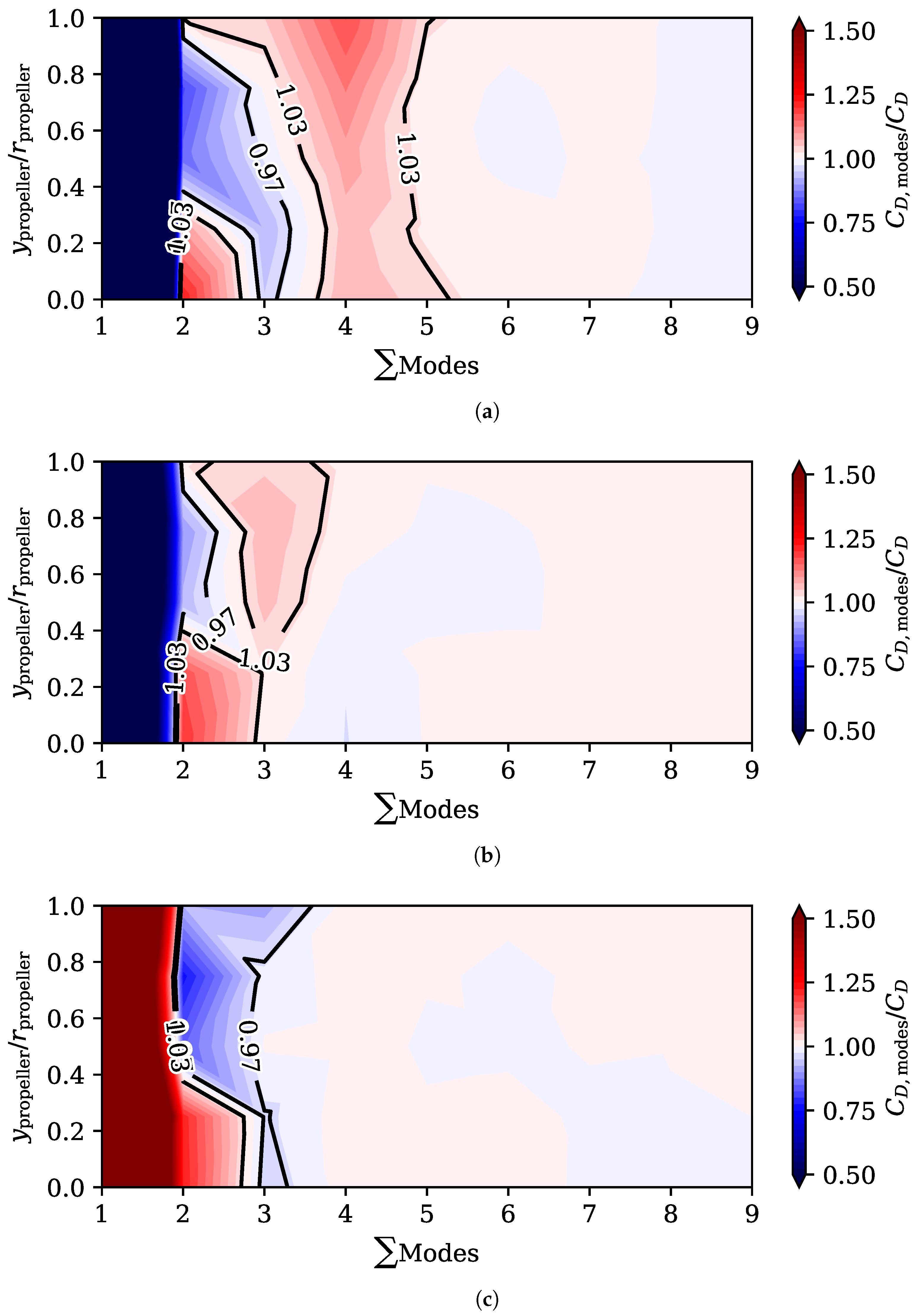
4.3. Lift and Drag Coefficient Analysis and Reconstruction
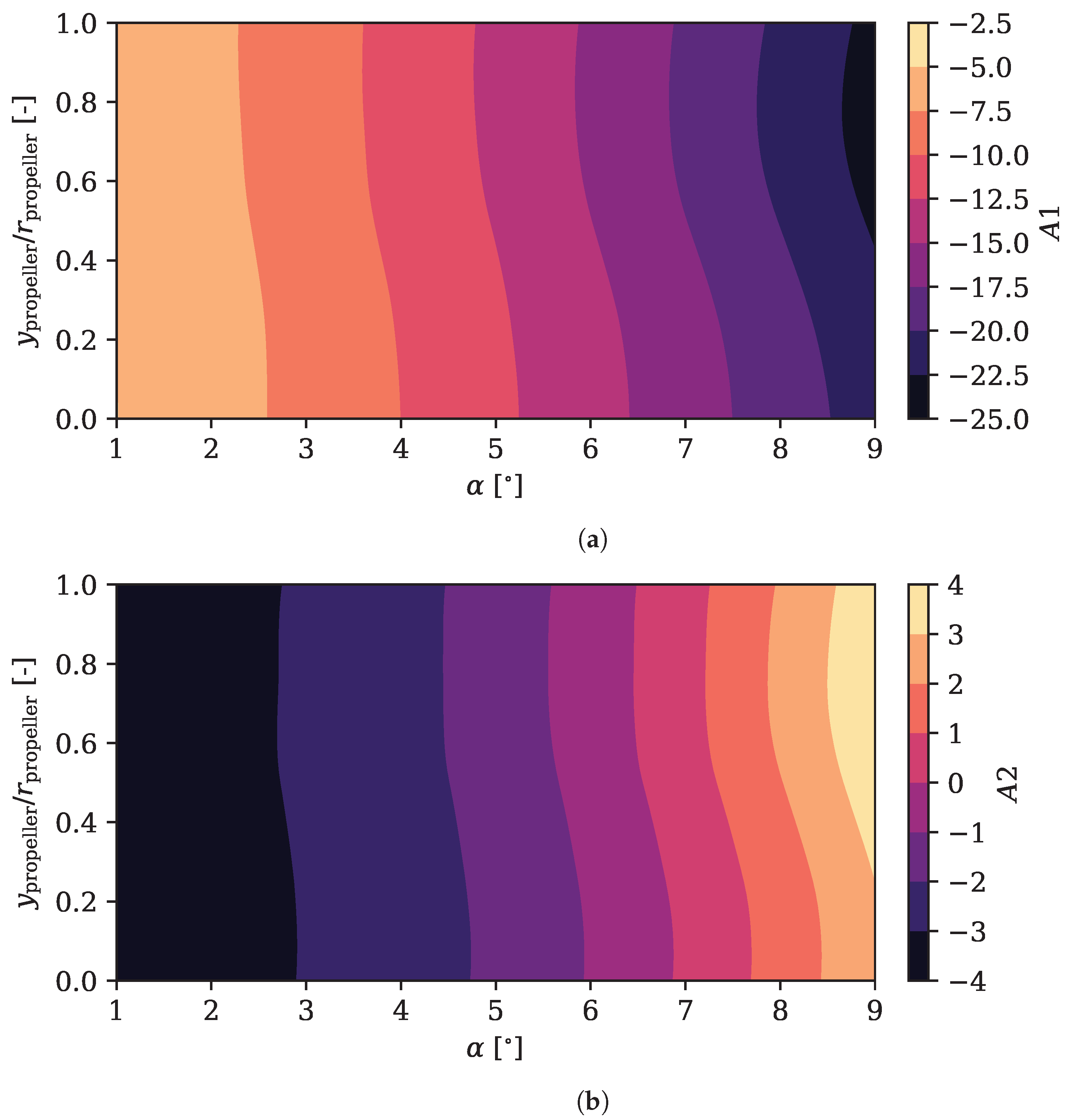
It is helpful to know how the coefficients of lift and drag behave as a function of the angle of attack and the position of the propeller. In Figure 19 and Figure 20, these two coefficients are represented as a function of the relative height of the actuator disc and the angle of attack of the aircraft for a Reynolds number of 5 × 10⁵.
Both C L and C D vary more with the angle of attack than with the propeller height over the trailing edge. Although both increase in magnitude with the angle of attack for a given position, they have opposite trends when the position is varied for a given angle of attack.
For a given angle of attack, as the propeller rises, the lift over the wing is greater while the drag is minimised. That is why the aerodynamic efficiency is maximised in the highest positions for any angle of attack, as shown in [25].
The pressure and friction coefficients have been integrated to obtain the lift and drag coefficients, where this operation has been carried out taking into account a different number of modes. The fractions of the lift coefficient and drag coefficient obtained doing the reconstruction with different number of modes, C L , modes / C L and C D , modes / C D , have been computed and they are shown in Figure 21 and Figure 22. The error results are shown depending on the number of modes used and the position of the propeller for a fixed angle of attack.
It is possible to observe in Figure 21 that the relative error when using two modes is less than 3% in the case of C L for many configurations. The error in this variable varies little with the position of the propeller, but it does for the angle of attack, where more modes are necessary to reduce the error at a low angle. At high angles of attack, using just 2 modes results in an overestimated C L , while at low angles of attack, the opposite occurs. As a general rule, at least five modes reduce the error by around 1%.
Figure 22 shows that the drag coefficient needs more modes than the lift coefficient to be reconstructed with low error. If a single mode is used, the error exceeds 50% at any angle of attack. When using 2 or 3 modes, the error remains at 3% and varies from overestimated at low propeller positions to underestimated at higher positions. As in the case of the C L , more modes are necessary at a lower angle of attack to maintain a C D relative error under 3%. At least 6 modes are required to represent any angle of attack correctly.

4.4. Interpolation of C p and C f with a Surrogate Model

The POD results are not only used to analyse the pressure and friction coefficients over the wing. As in other applications, they are also used to reduce the number of high fidelity simulations that it takes to fit a surrogate model. Once the modes for all propeller positions and angle of attack have been calculated, it is possible to interpolate and reconstruct the pressure and friction coefficients for any not-simulated intermediate cases, as shown in Figure 23 and Figure 24.
In Figure 23, the configuration coefficients of the POD are interpolated and the pressure coefficient is computed using the interpolated values and the modes of the decomposition. At 3 °, Reynolds of 5 × 10⁵, the positions of 30% and 65% are perfectly reconstructed, except for the C p closest to the propeller. For practical purposes, the contribution of the pressure distribution over the lift, drag and pitching moment coefficients over the wing are reconstructed with a very small error, but also the stresses over the the skin can be computed with high accuracy.
However, in Figure 24, where an angle of attack not used to fit the interpolator, an adequate reconstruction of the appearance of the recirculation bubble is not obtained, although the rest of the C p is correctly described. The stresses over the wing skin can still be computed with high accuracy with this interpolation.
In the same way, it is possible to represent the C f in Figure 25 and Figure 26.
In Figure 25, it can be seen that, for 3°, as it happened with the C p , the reconstruction of C f is perfect. In comparison, for 5.5 ° and in Figure 26, the reconstructed recirculation bubble is delayed with respect to that of the CFD simulations. The rest of the C f distribution is represented correctly.
The use of POD to reconstruct aerodynamic coefficients with low error interpolating a surrogate model is useful both in the pre-design and while optimising the wings of light UAVs. Light UAVs may be built using materials with very low stiffness, so a precise value of the pressure distribution over the wing is needed to optimise its structure without incurring in non-acceptable deformations of its shape.

5. Conclusions

After computing the pressure and friction coefficients over a wing section for different propeller positions and angles of attack, a modal decomposition using POD was performed. Looking at the data, more than 90% of the TKE is explained by the first mode of both the pressure and skin friction coefficients, for both the suction side and the pressure side of the airfoil. This means that, although some details are only described by taking into account higher-order modes, the main behaviour can be analysed by just looking at the first mode. From that, the main parameter affecting the distributions is the angle of attack, although the effect of the propeller position is not negligible.
For the pressure coefficient, rising the position of the propeller increases both the suction over the extrados and the overpressure over the intrados. The effect is similar to increasing the angle of attack, and explains an increment of lift between 10% to 20%. When the position is too high, with the shaft separated from the trailing edge a distance equal to the propeller radius, the trend is inverted and the extra lift starts to decrease. This is consistent with a decrease of the boundary layer ingestion effects.
But not only extra lift is produced: the suction peak is also moved towards the leading edge, decreasing the form drag due to the pressure distribution and creating some leading edge thrust. At the pressure side and higher modes, the trend due to the propeller position is not so obvious.
The nonlinear effects due to the propeller position are more obvious when looking at the skin friction coefficient. The maximum effects are seen for a position of around 70% for the first mode, which carries most of the information to reconstruct the coefficient distribution. For higher modes, no clear trend is found.
In order to reconstruct the LSB in the pressure coefficient over the airfoil, several higher modes are needed. For the friction coefficient, the case is more extreme, and up to ten modes are needed to fully catch the boundary layer transition due to the separation bubble.
By integrating the coefficients of pressure and friction, it is possible to obtain the coefficient of lift and drag for any combination of angle of attack and propeller position. Using at least two modes, it is possible to represent these coefficients below 3% of relative error in many cases, being necessary at least 6 modes for the error to fall below 1%.
The results of the modal decomposition can be used to fit surrogate models for optimisations for which the pressure or friction coefficient distribution is critical, such as when designing low-stiffness wing structures in small UAVs. In those cases, the pressure distribution has to be taken into account to get the exact load distribution over the skin, which may produce prohibitive deformations in some cases. Although some details are not accurately reconstructed in some configurations using this method, such as the exact shape of the transitional bubble, most of the coefficient distribution is obtained with negligible errors.

Author Contributions

Conceptualization, L.M.G.-C., P.V.; Data curation, P.V.; Formal analysis, P.V.; Funding acquisition, J.R.S., L.M.G.-C.; Investigation, P.V.; Methodology, L.M.G.-C., P.V.; Project administration, L.M.G.-C.; Resources, J.R.S.; Software, L.M.G.-C. and P.V.; Supervision, L.M.G.-C.; Validation, L.M.G.-C. and P.V.; Visualization, L.M.G.-C. and P.V.; Writing—original draft, P.V.; Writing—review and editing, J.R.S., L.M.G.-C., P.B. and P.V. All authors have read and agreed to the published version of the manuscript.

Funding

This work was partially funded by the Conselleria d’Innovació, Universitats, Ciència i Societat Digital of the Generalitat Valenciana through grant with expedient number GV/2021/069 of the program for “Grupos de Investigación Emergentes GV/2021”. This work is part of the project PID2020-119468RA-I00 funded by MCIN/AEI/10.13039/501100011033. This work is also part of the project EQC2019-006272-P funded by MCIN/AEI/10.13039/501100011033 and by “ERDF A way of making Europe”.

Institutional Review Board Statement

Not applicable.

Informed Consent Statement

Not applicable.

Data Availability Statement

The data presented in this study are available on request from the corresponding author.

Acknowledgments

The authors would like to thank L. Ricarte for his contribution to the work during the completion of his master’s thesis.

Conflicts of Interest

The authors declare no conflict of interest. The funders had no role in the design of the study; in the collection, analyses, or interpretation of data; in the writing of the manuscript, or in the decision to publish the results.

Abbreviations

The following abbreviations are used in this manuscript:
Abbreviations
BCGBoston Consulting Group
BLIBoundary layer ingestion
BEMTBlade Element Model Theory
CFDComputational fluid dynamics
DEPDistributed electrical propulsion
ERAEnvironmentally Responsible Aviation
HEHybrid electric
ITDSInformation Technology Development Solutions
LSBLaminar separation bubble
NASANational Aeronautics and Space Administration
PODProper Orthogonal Decomposition
RANSReynols-averaged Navier-Stokes
UAVUnmanned aerial vehicle
Roman letters
A Configuration coefficients matrix
a i Configuration coefficient of mode i
🜇Aspect ratio
bWingspan
cChord
C Covariance matrix
C L Lift coefficient
C D Drag coefficient
C D , 0 , extra Parasitic drag coefficient of the aircraft without the wing
C D , 0 , wing Parasitic drag coefficient of the wing
C p Pressure coefficient
C f Friction coefficient
DDrag
eOswald efficiency factor
hRelative height of the propeller shaft
r propeller Propeller radius
R e Reynolds
SWing surface
TThrust
TKE Total fluctuating kinetic energy
U Dataset matrix
U Air speed
xPosition across the chord
y propeller Position of the propeller shaft above the trailing edge
Greek letters
α Angle of attack
ΛEigenvalues matrix
λ Eigenvalue
ΦEigenvector matrix
ϕ Eigenvector
ρ Density

References

  1. Nickol, C.L.; Haller, W.J. Assessment of the performance potential of advanced subsonic transport concepts for NASA’s environmentally responsible aviation project. In Proceedings of the 54th AIAA Aerospace Sciences Meeting, San Diego, CA, USA, 4–8 January 2016; pp. 1–21. [Google Scholar] [CrossRef] [Green Version]
  2. Amoukteh, A.; Janda, J.; Vicent, J. Drones Go to work. Harv. Bus. Rev. 2017, 77–94. [Google Scholar]
  3. Kim, H.D.; Perry, A.T.; Ansell, P.J. A Review of Distributed Electric Propulsion Concepts for Air Vehicle Technology. In Proceedings of the AIAA/IEEE Electric Aircraft Technologies Symposium, Cincinnati, OH, USA, 9–11 July 2018; pp. 1–21. [Google Scholar] [CrossRef] [Green Version]
  4. Ko, Y.Y.A. The Multidisciplinary Design Optimization of a Distributed Propulsion Blended-Wing-Body Aircraft. Ph.D. Thesis, Virginia Tech, Blacksburg, Virginia, 2003. [Google Scholar]
  5. Moore, K.R.; Ning, A. Distributed electric propulsion effects on traditional aircraft through multidisciplinary optimization. In Proceedings of the AIAA/ASCE/AHS/ASC Structures, Structural Dynamics, and Materials Conference, Kissimmee, FL, USA, 8–12 January 2018. [Google Scholar] [CrossRef] [Green Version]
  6. Kirner, R.; Raffaelli, L.; Rolt, A.; Laskaridis, P.; Doulgeris, G.; Singh, R. An assessment of distributed propulsion: Part B—Advanced propulsion system architectures for blended wing body aircraft configurations. Aerosp. Sci. Technol. 2016, 50, 212–219. [Google Scholar] [CrossRef]
  7. Stoll, A.M.; Bevirt, J.; Moore, M.D.; Fredericks, W.J.; Borer, N.K. Drag Reduction Through Distributed Electric Propulsion. In Proceedings of the 14th AIAA Aviation Technology, Integration, and Operations Conference, Atlanta, GA, USA, 16–20 June 2014; pp. 1–10. [Google Scholar] [CrossRef] [Green Version]
  8. Stoll, A.M. Comparison of CFD and experimental results of the leap tech distributed electric propulsion blown wing. In Proceedings of the 15th AIAA Aviation Technology, Integration, and Operations Conference, Dallas, TX, USA, 22–26 June 2015; pp. 22–26. [Google Scholar] [CrossRef] [Green Version]
  9. Amoozgar, M.; Friswell, M.I.; Fazelzadeh, S.A.; Khodaparast, H.H.; Mazidi, A.; Cooper, J.E. Aeroelastic stability analysis of electric aircraft wings with distributed electric propulsors. Aerospace 2021, 8, 100. [Google Scholar] [CrossRef]
  10. Ausserer, J.K.; Harmon, F.G. Integration, validation, and testing of a hybrid-electric propulsion system for a small remotely-piloted aircraft. In Proceedings of the 10th Annual International Energy Conversion Engineering Conference, Atlanta, GA, USA, 30 July–1 August 2012; pp. 1–11. [Google Scholar] [CrossRef]
  11. Kim, C.; Namgoong, E.; Lee, S.; Kim, T.; Kim, H. Fuel Economy Optimization for Parallel Hybrid Vehicles with CVT; SAE Technical Paper 1999-01-1148; SAE International: Warrendale, PA, USA, 1999. [Google Scholar] [CrossRef]
  12. Budziszewski, N.; Friedrichs, J. Modelling of a boundary layer ingesting propulsor. Energies 2018, 11, 708. [Google Scholar] [CrossRef] [Green Version]
  13. Teperin, L. Investigation on Boundary Layer Ingestion Propulsion for UAVs. In Proceedings of the International Micro Air Vehicle Conference and Flight Competition (IMAV), Toulouse, France, 18–21 September 2017; pp. 293–300. [Google Scholar]
  14. Elsalamony, M.; Teperin, L. 2D Numerical Investigation of Boundary Layer Ingestion Propulsor on Airfoil. In Proceedings of the 7th European Conference for Aeronautics and Space Sciences (EUCASS), Milan, Italy, 3–6 July 2017; pp. 1–11. [Google Scholar] [CrossRef]
  15. Hall, D.K.; Huang, A.C.; Uranga, A.; Greitzer, E.M.; Drela, M.; Sato, S. Boundary layer ingestion propulsion benefit for transport aircraft. J. Propuls. Power 2017, 33, 1118–1129. [Google Scholar] [CrossRef]
  16. Broatch, A.; García-Tíscar, J.; Roig, F.; Sharma, S. Dynamic mode decomposition of the acoustic field in radial compressors. Aerosp. Sci. Technol. 2019, 90, 388–400. [Google Scholar] [CrossRef]
  17. Torregrosa, A.J.; Broatch, A.; García-Tíscar, J.; Gomez-Soriano, J. Modal decomposition of the unsteady flow field in compression-ignited combustion chambers. Combust. Flame 2018, 188, 469–482. [Google Scholar] [CrossRef]
  18. Zhu, Z.; Midlam-Mohler, S.; Canova, M. Development of physics-based three-way catalytic converter model for real-time distributed temperature prediction using proper orthogonal decomposition and collocation. Int. J. Engine Res. 2021, 22, 873–889. [Google Scholar] [CrossRef]
  19. Rulli, F.; Fontanesi, S.; D’Adamo, A.; Berni, F. A critical review of flow field analysis methods involving proper orthogonal decomposition and quadruple proper orthogonal decomposition for internal combustion engines. Int. J. Engine Res. 2021, 22, 222–242. [Google Scholar] [CrossRef] [Green Version]
  20. Shen, L.; Teh, K.Y.; Ge, P.; Zhao, F.; Hung, D.L. Temporal evolution analysis of in-cylinder flow by means of proper orthogonal decomposition. Int. J. Engine Res. 2021, 22, 1714–1730. [Google Scholar] [CrossRef]
  21. Malouin, B.; Trépanier, J.Y.; Gariépy, M. Interpolation of transonic flows using a proper orthogonal decomposition method. Int. J. Aerosp. Eng. 2013, 2013. [Google Scholar] [CrossRef]
  22. Mifsud, M.; Zimmermann, R.; Görtz, S. Speeding-up the computation of high-lift aerodynamics using a residual-based reduced-order model. CEAS Aeronaut. J. 2015, 6, 3–16. [Google Scholar] [CrossRef]
  23. Mifsud, M.J.; MacManus, D.G.; Shaw, S.T. A variable-fidelity aerodynamic model using proper orthogonal decomposition. Int. J. Numer. Methods Fluids 2016, 82, 646–663. [Google Scholar] [CrossRef] [Green Version]
  24. Tiseira, A.O.; García-Cuevas, L.M.; Quintero, P.; Varela, P. Series-hybridisation, distributed electric propulsion and boundary layer ingestion in long-endurance, small remotely piloted aircraft: Fuel consumption improvements. Aerosp. Sci. Technol. 2022, 120. [Google Scholar] [CrossRef]
  25. Serrano, J.R.; Tiseira, A.O.; García-Cuevas, L.M.; Varela, P. Computational Study of the Propeller Position Effects in Wing-Mounted, Distributed Electric Propulsion with Boundary Layer Ingestion in a 25 kg Remotely Piloted Aircraft. Drones 2021, 5, 56. [Google Scholar] [CrossRef]
  26. UAV Factory USA LLC. Penguin C UAS. Available online: https://www.uavfactory.com (accessed on 12 January 2012).
  27. AERTEC Solutions. RPAS TARSIS 25. Available online: https://aertecsolutions.com/rpas/rpas-sistema-aereos-tripulados-remotamente/rpas-tarsis25/ (accessed on 12 January 2012).
  28. Lyon, C.A.; Broeren, A.P.; Giguere, P.; Gopalarathnam, A.; Selig, M.S. Summary of Low-Speed Airfoil Data—Volume 3; SoarTech Publications: Virginia Beach, VA, USA, 1997; p. 315. [Google Scholar]
  29. Selig, M.S.; Donovan, J.F.; Fraser, D.B. Airfoils at Low Speeds; H.A. Stokey: Virginia Beach, VA, USA, 1989; pp. 1–408. [Google Scholar]
  30. Selig, M.S. Low Reynolds Number Airfoil Design Lecture Notes—Various Approaches to Airfoil Design. Available online: https://m-selig.ae.illinois.edu/pubs/Selig-2003-VKI-LRN-Airfoil-Design-Lecture-Series.pdf (accessed on 12 January 2012).
  31. Sutton, D.M. Experimental Characterization of the Effects of Freestream Turbulence Intensity on the SD7003 Airfoil at Low Reynolds Numbers. Master’s Thesis, Univeristy of Toronto, Toronto, ON, Canada, 2015. [Google Scholar]
  32. Ananda, G.K.; Sukumar, P.P.; Selig, M.S. Measured aerodynamic characteristics of wings at low Reynolds numbers. Aerosp. Sci. Technol. 2015, 42, 392–406. [Google Scholar] [CrossRef]
  33. Stajuda, M.; Obidowski, D.; Karczewski, M.; Józwik, K. Modified virtual blade method for propeller modelling. Mech. Mech. Eng. 2018, 22, 603–617. [Google Scholar] [CrossRef]
  34. Harmon, F.G.; Frank, A.A.; Chattot, J.J. Conceptual design and simulation of a small hybrid-electric unmanned aerial vehicle. J. Aircr. 2006, 43, 1490–1498. [Google Scholar] [CrossRef]
  35. Niţă, M.; Scholz, D. Estimating the Oswald Factor from Basic Aircraft Geometrical Parameters. In Deutscher Luft- und Raumfahrtkongress; DGLR: Berlin, Germany, 2012. [Google Scholar]
  36. Hoerner, S. Fluid-Dynamic Drag; Hoerner Fluid Dynamics: Bakersfield, CA, USA, 1965; pp. 7-2–7-9. [Google Scholar]
  37. XFLR5. Available online: https://www.xflr5.tech/xflr5.htm (accessed on 12 January 2012).
  38. Drela, M. XFOIL Subsonic Airfoil Development System. Available online: https://web.mit.edu/drela/Public/web/xfoil/ (accessed on 12 January 2012).
Figure 1. Simulated aircraft, as shown in [24]. This sketch is for a configuration of 12 propellers.
Drones 06 00038 g001
Figure 2. Side view sketch of the computational grid used for the current calculations.
Drones 06 00038 g002
Figure 3. Airfoil side-view with principal heights (not to scale).
Drones 06 00038 g003
Figure 4. Maximum and minimum propeller heights above the trailing edge. (a) Section of wing simulated with a virtual disc for modelling the propeller. (b) 0% position. (c) 100% position.
Drones 06 00038 g004
Figure 5. Front section of the analysed airfoil section, marked in blue.
Drones 06 00038 g005
Figure 6. Pressure coefficient distribution at two angles of attack for a Reynolds number of 5 × 10⁵ and a propeller position of 75%.
Drones 06 00038 g006
Figure 7. TKE of the different C p modes for both the suction side (in blue) and pressure side (in red).
Drones 06 00038 g007
Figure 8. First four modes of the pressure coefficient of the suction side.
Drones 06 00038 g008
Figure 9. First four modes of the pressure coefficient of the pressure side.
Drones 06 00038 g009
Figure 10. Pressure coefficient over the airfoil for an angle of attack of 3°, a propeller position of 50%. The results for the reconstruction with the first 3 and 9 eigenvectors are also included.
Drones 06 00038 g010
Figure 11. Configuration coefficients for the first two modes of the pressure coefficient over the suction side of the airfoil, as a function of the angle of attack and the relative propeller position. (a) Configuration coefficient A 1 of the first mode of C p over the suction side. (b) Configuration coefficient A 2 of the second mode of C p over the suction side.
Drones 06 00038 g011
Figure 12. Contribution of the two first modes in the case of maximum relative height of the propeller over the trailing edge and maximum angle of attack simulated.
Drones 06 00038 g012
Figure 13. Configuration coefficients for the first three modes of the pressure coefficient over the pressure side of the airfoil, as a function of the angle of attack and the relative propeller position. (a) Configuration coefficient A 1 of the first mode of the pressure coefficient over the pressure side. (b) Configuration coefficient A 2 of the second mode of the pressure coefficient over the pressure side. (c) Configuration coefficient A 3 of the third mode of the pressure coefficient over the pressure side.
Drones 06 00038 g013
Figure 14. Friction coefficient over the airfoil with the propeller in 50% position.
Drones 06 00038 g014
Figure 15. TKE of the friction coefficient.
Drones 06 00038 g015
Figure 16. Friction coefficient reconstruction over the airfoil, for an angle of attack of 3° and a propeller relative height of 50%. (a) Friction coefficient reconstruction over the suction side of the airfoil. (b) Friction coefficient reconstruction over the pressure side of the airfoil.
Drones 06 00038 g016
Figure 17. Configuration coefficients for the first two modes of the friction coefficient over the suction side of the airfoil, as a function of the angle of attack and the relative propeller position. (a) Configuration coefficient A 1 of the first mode of the friction coefficient over the suction side. (b) Configuration coefficient A 2 of the second mode of the friction coefficient over the suction side.
Drones 06 00038 g017
Figure 18. Configuration coefficients for the first two modes of the friction coefficient over the pressure side of the airfoil, as a function of the angle of attack and the relative propeller position. (a) Configuration coefficient A 1 of the first mode of the friction coefficient over the pressure side. (b) Configuration coefficient A 2 of the second mode of the friction coefficient over the pressure side.
Drones 06 00038 g018
Figure 19. Lift coefficient for each propeller position above the trailing edge and angle of attack.
Drones 06 00038 g019
Figure 20. Drag coefficient for each propeller position above the trailing edge and angle of attack.
Drones 06 00038 g020
Figure 21. Fraction of lift coefficient computed using from 1 to 9 modes, using both the pressure coefficient and friction coefficient distributions. (a) Lift coefficient computed using from 1 to 9 modes for an angle of attack of 1°. (b) Fraction of lift coefficient computed using from 1 to 9 modes for an angle of attack of 5°. (c) Fraction of lift coefficient computed using from 1 to 9 modes for an angle of attack of 9°.
Drones 06 00038 g021
Figure 22. Fraction of drag coefficient computed using from 1 to 9 modes, using both the pressure coefficient and friction coefficient distributions. (a) Fraction of drag coefficient computed using from 1 to 9 modes for an angle of attack of 1°. (b) Fraction of drag coefficient computed using from 1 to 9 modes for an angle of attack of 5°. (c) Fraction of drag coefficient computed using from 1 to 9 modes for an angle of attack of 9°.
Drones 06 00038 g022
Figure 23. Pressure coefficient reconstructed in a propeller position not used to fit the surrogate model, compared with data from a CFD simulation. (a) Pressure coefficient reconstructed an angle of attack of 3° and a propeller position of 30%. (b) Pressure coefficient reconstructed for an angle of attack of 3° and a propeller position of 65%.
Drones 06 00038 g023
Figure 24. Pressure coefficient reconstructed in a propeller position and angle of attack not used to fit the surrogate model, compared with data from a CFD simulation. (a) Pressure coefficient reconstructed for an angle of attack of 5.5 ° and a propeller position of 50%. (b) Pressure coefficient reconstructed for an angle of attack of 5.5 ° and a propeller position of 65%.
Drones 06 00038 g024
Figure 25. Friction coefficient reconstructed in a propeller position not used to produce the surrogate model, compared with data from a CFD simulation. (a) Friction coefficient reconstructed an angle of attack of 3° and a propeller position of 30%. (b) Friction coefficient reconstructed for an angle of attack of 3° and a propeller position of 65%.
Drones 06 00038 g025
Figure 26. Friction coefficient reconstructed in a propeller position and angle of attack not used to fit the surrogate model, compared with data from a CFD simulation. (a) Friction coefficient reconstructed for an angle of attack of 5.5 ° and a propeller position of 50%. (b) Friction coefficient reconstructed for an angle of attack of 5.5 ° and a propeller position of 65%.
Drones 06 00038 g026
Table 1. Aircraft data.
Design Parameters
Aspect ratio10
Wing area 0.4   m 2
Wingspan m
Wing chord 0.2   m
Maximum takeoff mass25  k g
Wing airfoilSD7003
Propeller radius40  m m
Number of propellers13
Aerodynamic Parameters
C D , 0 , extra (fuselage, empennage, others)0.011
Oswald efficiency factor (e)0.8
Publisher’s Note: MDPI stays neutral with regard to jurisdictional claims in published maps and institutional affiliations.

