
Design and Implementation of a UUV Tracking Algorithm for a USV


Maritime Technology Research Institute, Agency for Defense Development, Changwon 51678, Korea
*
Author to whom correspondence should be addressed.
Drones 2022, 6(3), 66; https://0-doi-org.brum.beds.ac.uk/10.3390/drones6030066
Submission received: 11 February 2022
/
Revised: 28 February 2022
/
Accepted: 1 March 2022
/
Published: 2 March 2022
(This article belongs to the Topic Autonomy for Enabling the Next Generation of UAVs)
Abstract
:In a departure from the past, unmanned underwater vehicles (UUVs) and unmanned surface vehicles (USVs) are increasingly needed for complementary cooperation in military, scientific, and commercial applications, because this is more efficient than standalone operations. Information sharing through acoustic underwater communication is vital for complementary cooperation between USVs and UUVs. Normally, since USVs have advantages in terms of wide operational boundaries compared to UUVs, they are efficient for tracking UUVs. In this paper, we suggest a UUV tracking algorithm for a USV. The tracking algorithm’s development consists of three main software models: an estimation based on an extended Kalman filter (EKF) with a navigation smoothing method, guidance based on multimode guidance, and re-searching based on a pattern. In addition, the algorithm provides a procedure for tracking UUVs in complex acoustic underwater communication environments. The tracking algorithm was tested in a simulated environment to check the performance of each method, and implemented with a USV system to verify its validity and stability in sea trials. The UUV tracking algorithm of the USV shows stable and efficient performance.
1. Introduction
Until now, the operating concepts of unmanned surface vehicles (USVs) and unmanned underwater vehicles (UUVs) have been individually researched by connecting them to manned systems through a network to perform missions. In other words, USVs and UUVs acquire controlled and measured information over remote communication with each control center, and perform missions such as surface or underwater surveillance [1,2]. However, complementary cooperation between USVs and UUVs has recently been emphasized due to extensions of their range of operation [3]. In this complementary cooperation, the USV needs high performance (e.g., duration, velocity, payload, and navigation accuracy) compared to the UUV [4,5].
Previous methods of tracking UUVs have been proposed [6,7,8,9,10]. For example, Petter Norgren showed a tracking algorithm based on an estimated UUV position with acoustic modem telemetry and a mission plan [7]. José Melo’s research presented an estimation of a UUV’s position using two beacons over an acoustic underwater communication and a continuous–discrete Kalman filter for the UUV motion [10]. However, these studies are not sufficient for a complementary cooperation mission between a USV and UUV based on acoustic underwater communication. In an underwater environment, sound waves have been used for acoustic underwater communication. The sound waves have a low-frequency bandwidth and a sound speed. Moreover, the sound waves cause a delay, which spreads due to multipath reflections and frequency shifts as a result of the Doppler effect [11,12,13]. These limitations induce a loss of acoustic underwater communication, and cause long transmission times. In these situations, USVs need a tracking algorithm to follow UUVs stably.
This paper proposes a UUV tracking algorithm for a USV. This algorithm consists of three main software models that estimate the UUV states based on an extended Kalman filter (EKF) model with a navigation smoothing method, follow the UUV based on multimode guidance, and re-search for the UUV using a specific pattern. The control input of the EKF is modified by applying the navigation smoothing method in the acoustic underwater communication environment. The multimode guidance has two guidance modes to follow the UUV according to the distance between the UUV and the USV. In addition, the multimode guidance has a control function to maintain an optimal distance for acoustic underwater communication. The re-search model is designed to quickly find the UUV in the event of a loss of acoustic underwater communication.
Each of the three main software models of the UUV tracking algorithm was studied in a virtual simulation environment to reduce time and cost aspects. After finishing the simulation tests, the UUV tracking algorithm was applied to a USV and tested to verify its performance in a sea trial.
2. Algorithm Architecture
The application of this study was carried out in a USV called a U-Tracer, which is designed to chase underwater targets using sound navigation and ranging (SONAR); it was developed by the Agency for Defense Development (ADD), and is shown in Figure 1.
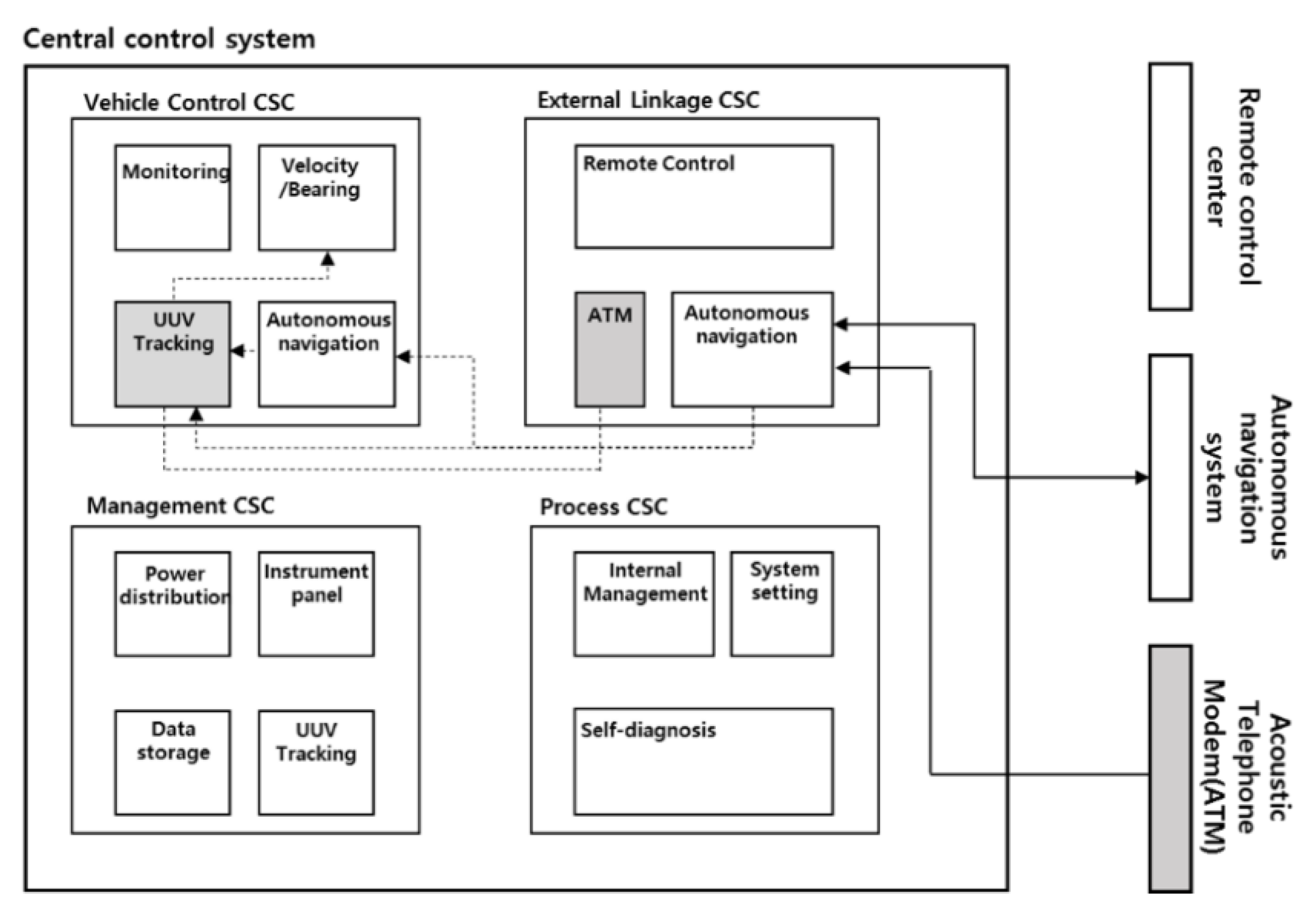
The UUV tracking algorithm, including the estimation, guidance, and re-search model, was added to a vehicle control computer software component (CSC) of a central control system that acts as the brain of the USV. In addition, for the acoustic underwater communication between the USV and UUV, an acoustic telephone modem (ATM) was installed on a strut instead of the SONAR. The ATM model was a Teledyne Benthos-916 with a communication distance of 4 km, a medium frequency range of 16–21 kHz, and a housing material depth of 500 m. Figure 2 shows a data flowchart related to the UUV tracking algorithm. The essential data for processing the UUV tracking algorithm are two pieces of navigation information: one is the USV navigation information received from the USV autonomous navigation system; the other is the UUV navigation information received from the UUV through the ATM. The tracking algorithm determines the USV command information (i.e., velocity and heading) in the next step.
Figure 3 shows the UUV tracking algorithm’s procedure. When receiving the start message from the remote control center, the UUV tracking algorithm starts operating. First, the algorithm checks for abnormalities in its reception of the UUV navigation information, and then estimates the UUV states (i.e., location , yaw [], and velocity []). If there are abnormalities, the algorithm counts the number of successive failures ( in the acoustic underwater communication. The guidance model sets the guidance mode and calculates command information if is lower than a certain value () set by the user. When , the algorithm goes to the re-search model to calculate the command information. Finally, the algorithm updates the command information of the USV in the next step. This procedure is repeated until it is terminated by the remote control center of the USV.
3. UUV Tracking Models and Simulation Results
3.1. Estimation Model
Due to the environmental characteristics of acoustic underwater communication, such as unstable connection and long communication time, it is difficult for the USV to estimate the UUV’s states (i.e., position, orientation, and velocity). This study describes a system model of the EKF based on an estimation smoothing method to overcome the lack of information caused by intermittent measurements of the UUV states [14,15,16,17,18,19,20]. The state vector and system model indicating the UUV states can be expressed as shown in Equations (1) and (2):
where represents the state variables (i.e., location , yaw ], and velocity ]) in step k, the nonlinear state transition function () represents how the system changes over time (), and is the system noise entering the system, which affects state variables.
The yaw rate () and velcocity rate () of the control input based on the navigation smoothing method are calculated using , which is the yaw rate and velocity rate in step, and , which is the average yaw rate and velocity rate over the previous instances. Here, is a specific number input by a user. Equation (3) exhibits the summarized yaw rate and velocity rate. Equation (4) shows the measurement model.
where represents the measurement values (i.e., location [, ], yaw [, and velocity ]) from the UUV through the acoustic underwater communication, denotes a nonlinear state transition function presenting the relationship between the measurement values and states variables, and is the measurement noise.
To test the estimation model, a Monte Carlo simulation was performed with the proposed model () compared to the constant EKF model. In the simulated scenario, the UUV maneuvers at a velocity of 5 knots on an ellipsoidal path with curves and straight lines, as shown in Figure 4. The execution cycle time of the estimation model is every second until the UUV goes around the path. It is assumed that the USV receives the UUV information () through acoustic underwater communication every 5 s. Table 1 defines random error variables.
The average of the root-mean-square error (RMSE) was calculated to evaluate both methods. The iteration number of the Monte Carlo simulation was 1000 times. Table 2 shows the results of the average of RMSE for the distance, yaw, and velocity. The proposed model-designed input control model is better than the constant EKF model. In particular, the distance and yaw of the proposed EKF are close to the real UUV states. The proposed EKF-designed input control model helps to estimate the UUV states, and ensures that the USV can track the UUV stably.
3.2. Guidance Model
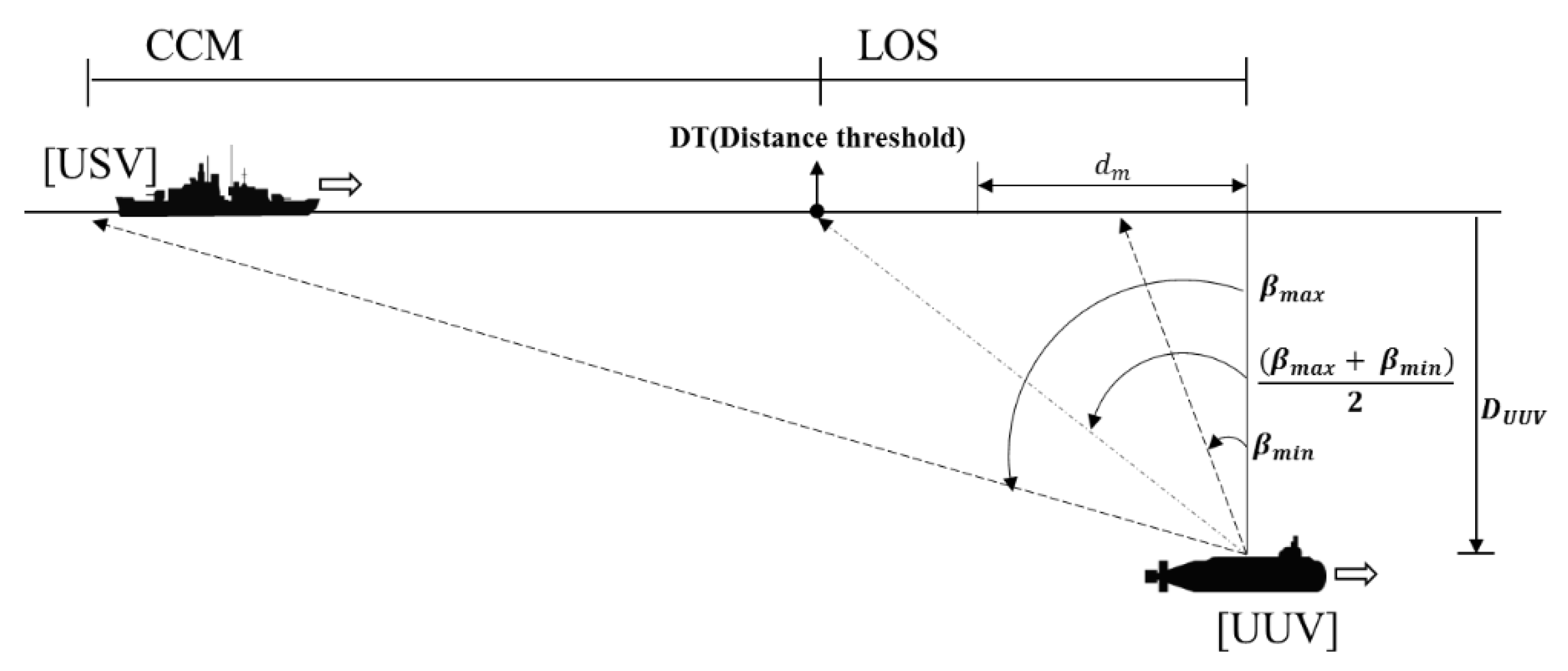
For the USV to cooperate with the UUV, it needs to follow the UUV quickly and stably. In this study, the multimode guidance model for following the UUV consists of two guidance methods: One form of multimode guidance is line-of-sight (LOS); this is a classical and simple technique for guiding a stationary target [21,22,23,24]. This technique of approaching the rear of the UUV is stable, since the velocity vector of the USV is always adjusted to face the UUV. However, this technique has difficulty approaching a UUV quickly when that UUV is performing complicated maneuvers or is far away from the USV [25]. Therefore, another guidance method called the collision course method (CCM) is used to solve these problems. The CCM is a general missile guidance technique [26,27] that calculates the angle of impact by reflecting a UUV’s velocity and course, and allows the USV to quickly approach the UUV. In consideration of the two methods’ strengths and weaknesses, multimode guidance selects one method depending on the separation distance between the USV and UUV. Equation (5) displays a simplified equation of the multimode guidance:
where DT is the distance threshold for switching from the CCM to LOS, and is determined according to the minimum ( and maximum operation angles ( of the ATM and the operation depth () of the UUV; is the minimum separation distance between the USV and UUV, and is the safe distance. Furthermore, denotes the separation distance between the USV and UUV, is the angle of the command heading for the USV in the next step, is the angle of the UUV from the USV, is the course of the UUV, and () are the velocities of the UUV and USV, respectively. Finally, k is the gain coefficient, and () are the positions of the UUV and USV, respectively. Figure 5 explicates the multimode guidance concept.
To evaluate the performance of the multimode guidance model, a simulation was performed with the following time (FT) and following stability (FS) as sub-measures of effectiveness (sub-MOE). The MOE is defined as the sum of two weighted sub-MOEs. The weight of each sub-MOE is assigned as shown in Table 3.
Equation (6) shows the summarized MOE (G.MOE) of the guidance model:
where n is the total number of simulations, and the following stability has a high score when the USV is located close to the rear of the USV.
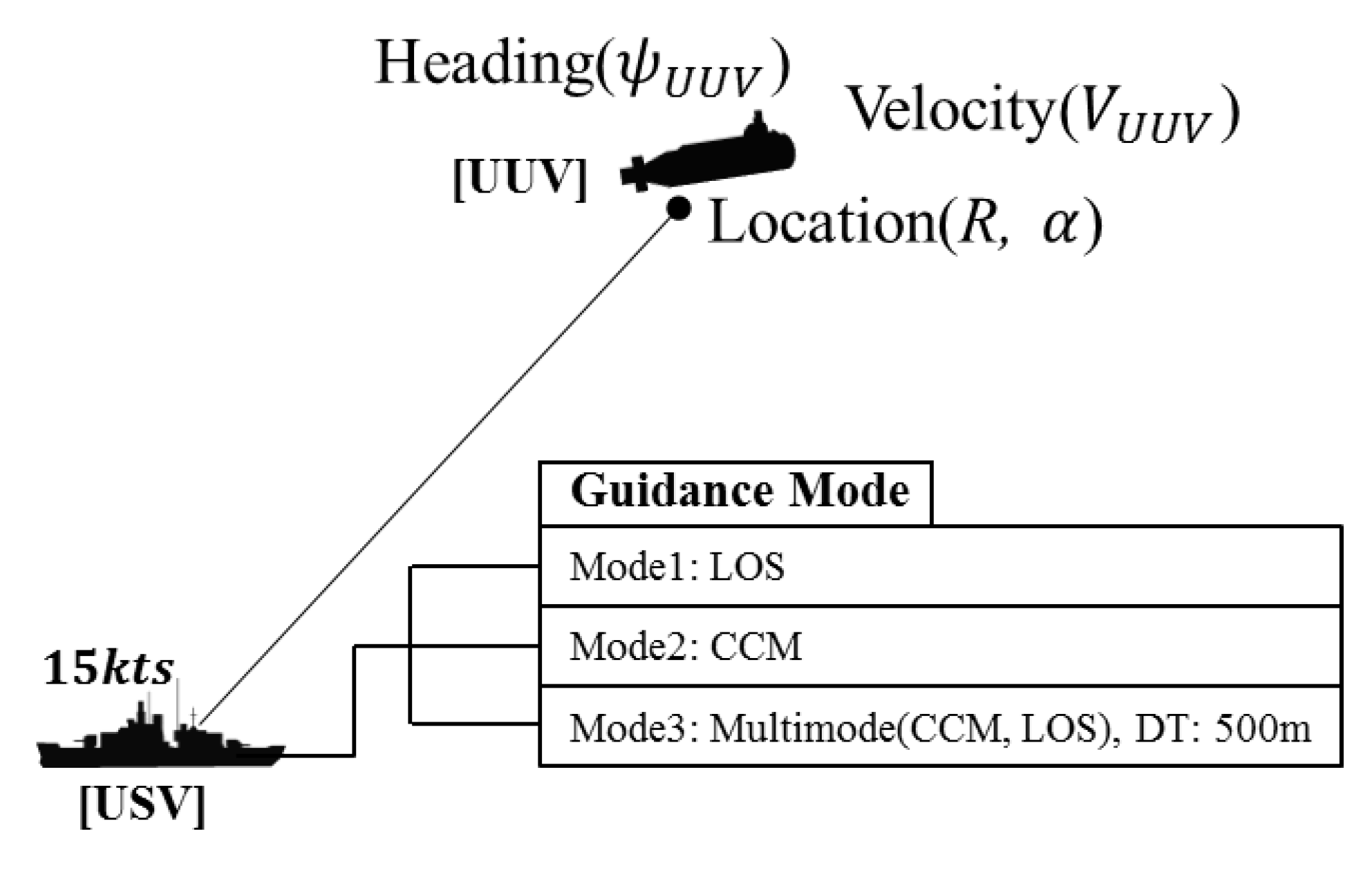
Figure 6 presents the simulation scenario. The simulation assumption is that the USV, traveling at 15 knots, follows the UUV after connecting via acoustic underwater communication. The UUV maneuvers in a straight line using the initial setting values of a heading angle and velocity, and the simulation end time is 3000 s. Table 4 defines the random error variables in the guidance simulation.
Figure 7 shows the results of the Monte Carlo simulations (10,000 times) for the three guidance modes. The CCM guidance mode requires less following time compared to others; this means that the USV can quickly approach the UUV. In the case of the following stability, the LOS guidance attains high scores, enabling the USV to follow the rear of the UUV stably. Considering the two important sub-MOEs comprehensively, the multimode guidance presents the most efficient result. By selecting the multimode guidance mode according to the separation distance between the USV and UUV, the USV reduces the approach time and maintains a stable position.
3.3. Re-Search Model
The USV needs to perform a re-search when it loses acoustic underwater communication with the UUV due to an unexpected situation. Appropriate re-search models have been widely studied [28,29,30,31]. Among them, Jeon’s research examines the effectiveness of various re-search patterns by analyzing the re-search success rate for various target speeds; the spiral and sector patterns are appropriate when the target velocity is under 10 knots [30]. The re-search time is an important sub-MOE for evaluating both of these re-search patterns. To select an efficient re-search pattern, we performed an effectiveness analysis with two sub-MOEs (re-search time and rate of re-search success), based on a simulation. The MOE is defined as the sum of two weighted sub-MOEs. Table 5 shows how the weight of each sub-MOE is assigned, and Equation (7) shows the summarized re-search MOE (R.MOE).
where n is the total number of simulations, RT is the re-search time (s), RR is the re-search success rate (%), and (, ) are the weights for RT and RR, respectively.
Figure 8 presents the simulation scenario. The simulation assumption is that the USV with 15 knots behind the UUV performs the re-search (i.e., sector or spiral pattern) after losing acoustic underwater communication. Table 6 defines the random error variables of the re-search simulation, and the simulation end time is 600 s. The condition of the re-search success is the distance (<500 m) between the USV and UUV.
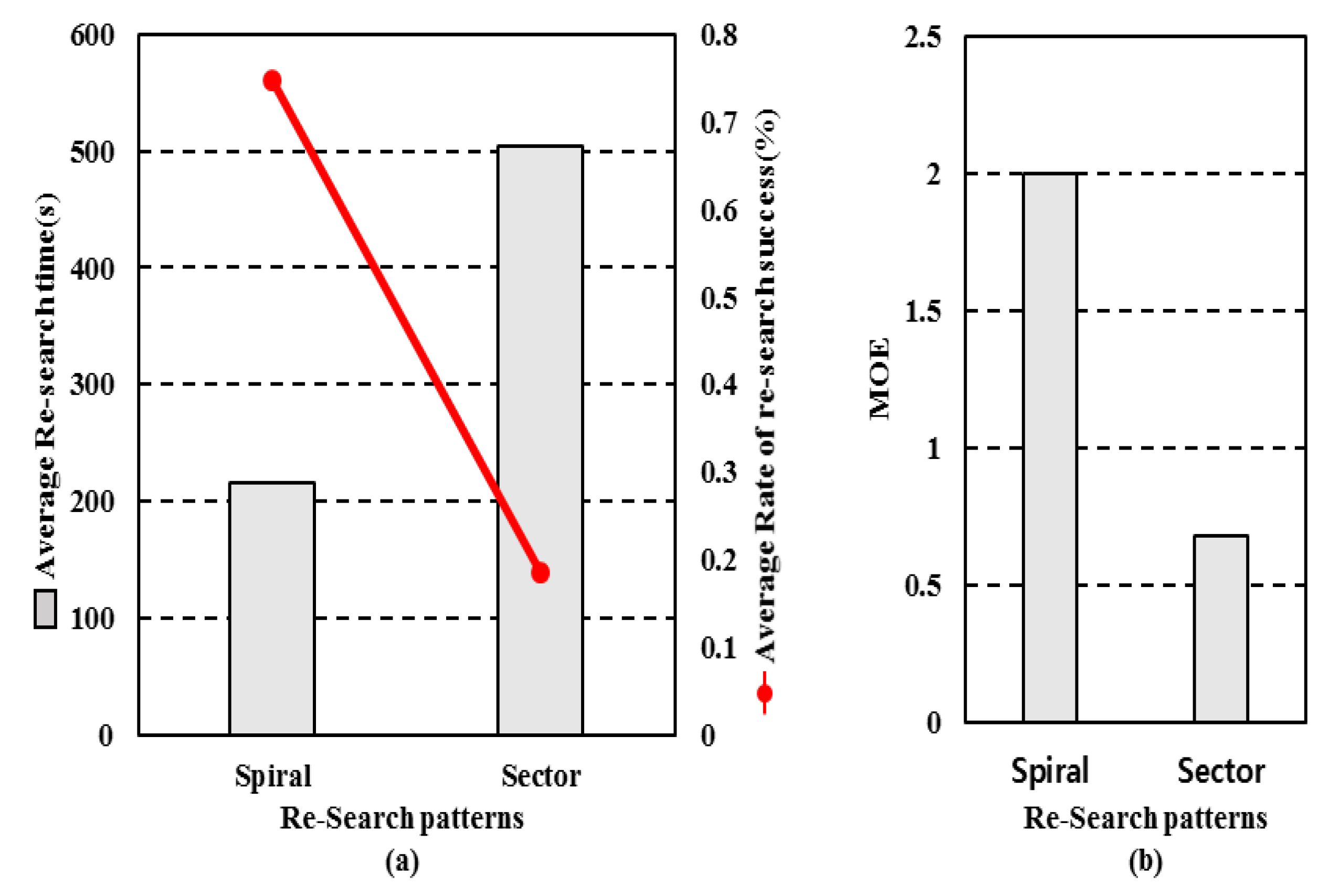
Figure 9 shows the results of the Monte Carlo simulations (1000 times) for the spiral and sector patterns. The spiral pattern has a higher average rate of re-search success than the sector pattern. In the case of the re-search time, the spiral pattern takes less time than the sector pattern on average. To measure the effectiveness by comprehensively calculating the two factors, the spiral pattern is ~1.96 times better than the sector pattern, because the spiral can re-search all orientations quicker than the sector pattern, with many straight re-search sections. As a result of these findings, the spiral pattern was applied with the re-search model.
4. Implementation and Results
A test of the tracking algorithm’s performance was carried out at sea in May 2020. The tracking algorithm was loaded into the vehicle control CSC of the U-Tracer USV. Since the UUV has not yet been developed, a virtual UUV was simulated and prepared to transmit the information about the virtual UUV states via radio communication from the USV control center to the USV. The purpose of this test was to validate the USV’s tracking stability. The conditions of the sea test were as shown in Table 7.
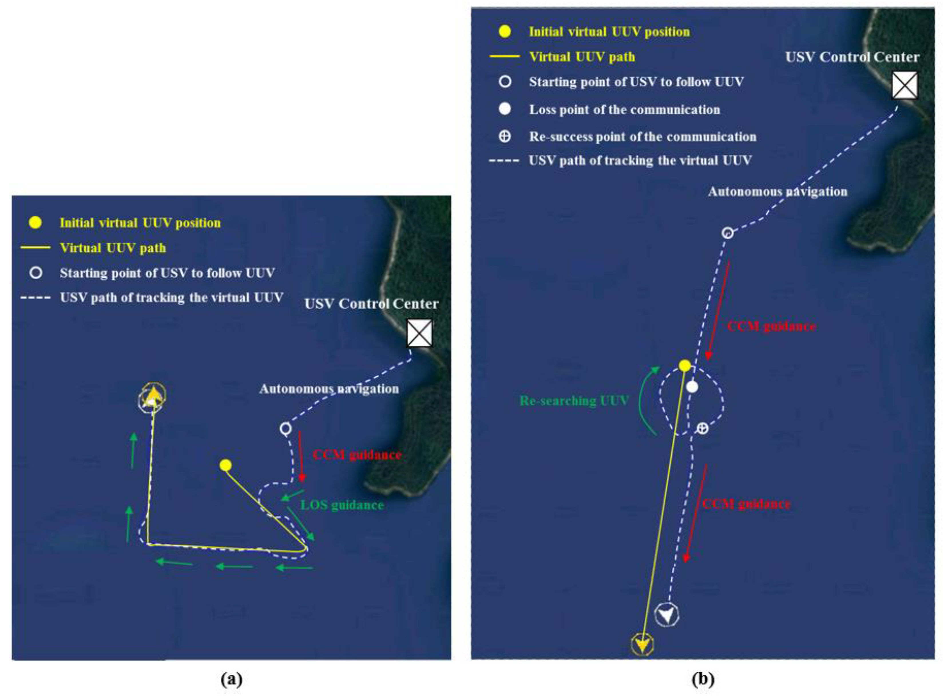
Figure 10a,b show the USV operation screens at the remote control center on land in case of Scenarios 1 and 2, respectively. In Scenario 1, the USV, at a velocity of 5 knots, was under autonomous navigation 350 m away from the virtual UUV, which operated at 4 knots and maneuvered in the shape of a triangle. After changing the autonomous navigation mode to the UUV tracking mode, the USV followed the virtual UUV to use the tracking algorithm. The guidance mode switched from CCM mode to LOS mode within the distance threshold of ~350 m. This result shows that the USV quickly approached the virtual UUV in CCM mode and stably followed the rear of the virtual UUV in LOS mode. In Scenario 2, the USV, at a velocity of 5 knots, was under autonomous navigation 350 m away from the virtual UUV, which operated at 4 knots and maneuvered in the shape of a straight line. The USV approached the virtual UUV in CCM mode until a communication breakdown. When , the USV performed the re-search in the spiral pattern to find the virtual UUV. After reconnecting the communication, the USV followed the virtual UUV in CCM mode. This result shows that the USV can perform the re-search in unexpected situations. In addition, in spite of periodically receiving virtual UUV states approximately every 5 s, the USV stably followed the rear of the virtual UUV while maintaining a desirable distance.
5. Conclusions and Future Work
The UUV tracking algorithm for the USV was designed and implemented for the acoustic underwater communication environment, which has unstable and long communication times for complementary cooperation between the USV and the UUV. The UUV tracking algorithm consists of the estimation model designed by the EKF with the smoothing method for estimating UUV states, the multimode guidance model for following the UUV, and the re-search model with the spiral pattern for re-searching the UUV when disconnected from acoustic communication for a certain amount of time. To verify the stability and validity of the proposed tracking algorithm, the performance of each model was tested based on the simulation environment. In the estimation model, the proposed EKF-designed input control model helps to estimate the UUV states, and ensures that the USV can track the UUV stably. In the multimode guidance model, the USV reduces the approach time and maintains a stable position according to the separation distance between the USV and UUV. In the re-search model, the spiral pattern is more efficient than the sector pattern because the spiral can re-search all orientations quickly. In addition, the algorithm was loaded onto the USV (U-Tracer) and tested using a virtual UUV on the sea. The USV followed and re-searched the virtual UUV while maintaining the proper distance and velocity, in spite of periodically receiving virtual UUV states approximately every 5 s and disconnecting the communication.
The global market for complementary cooperation between the USV and the UUV is expected to grow in the near future. Future work should explore how the USV cooperates with a developed UUV using the designed tracking algorithm on the sea. Furthermore, this study could contribute to investigations of the ocean floor, searching for sunken ships and aircraft, and monitoring marine life in the private sector.
Author Contributions
Conceptualization, J.-G.K.; methodology, J.-G.K. and T.K.; software, J.-G.K.; validation, J.-G.K., T.K., H.-D.K. and J.-S.P.; formal analysis, L.K. and H.-D.K.; investigation, L.K.; writing—original draft preparation, J.-G.K. and T.K.; writing—review and editing, J.-G.K., T.K. and L.K.; visualization, H.-D.K. and J.-S.P. All authors have read and agreed to the published version of the manuscript.
Funding
This research received funding for the project called “development of an autonomous control technology for an unmanned underwater vehicle based on surface and underwater cooperation” via grant 912614501.
Institutional Review Board Statement
Not applicable.
Informed Consent Statement
Not applicable.
Data Availability Statement
Not applicable.
Acknowledgments
The authors gratefully acknowledge the support of the Agency for Defense Development (ADD), the Republic of Korea. In addition, thanks are due to the editors and reviewers for contributing to the final form of this research.
Conflicts of Interest
The authors declare no conflict of interest.
References
- Sinisterra, A.; Dhanak, M.; Kouvaras, N. A USV Platform for Surface Autonomy. In Proceedings of the OCEANS 2017-Anchorage (IEEE), Anchorage, AK, USA, 18–21 September 2017; pp. 1–8. [Google Scholar]
- Allard, Y.; Shahbazian, E. Unmanned Underwater Vehicle (UUV) Information Study; OODA Technology Inc.: Montreal, QC, Canada, 2014. [Google Scholar]
- Savkin, A.V.; Verma, S.C.; Anstee, S. Optimal navigation of an unmanned surface vehicle and an autonomous underwater vehicle collaborating for reliable acoustic communication with collision avoidance. Drones 2022, 6, 27. [Google Scholar] [CrossRef]
- Martinez, J.L.; Brescia, A.; Mullen, L.; Mulligan, A.; Alley, D.; Lautrup, R.; Platt, D. NIX USV platform for precision track and trail of UUV platforms. Ocean Sens. Monit. XII 2020, 11420, 114200O. [Google Scholar]
- Cen, Y.; Liu, M.; Li, D.; Meng, K.; Xu, H. Double-scale adaptive transmission in time-varying channel for underwater acoustic sensor networks. Sensors 2021, 21, 2252. [Google Scholar] [CrossRef] [PubMed]
- Daxiong, J.; Rong, Z.; Ruiwen, Y.; Hongyu, Z.; Yang, L. A tracking control method of ASV following AUV. In Proceedings of the OCEANS 2014-San Diego (IEEE), San Diego, CA, USA, 23–27 September 2013; pp. 1–8. [Google Scholar]
- Norgren, P.; Ludvigsen, M.; Ingebretsen, T.; Hovstein, V.E. Tracking and remote monitoring of an autonomous underwater vehicle using an unmanned surface vehicle in the Trondheim fjord. In Proceedings of the OCEANS 2015-MTS/IEEE Washington (IEEE), Washington, DC, USA, 19–22 October 2015; pp. 1–6. [Google Scholar]
- Phillips, A.B.; Salavasidis, G.; Kingsland, M.; Harris, C.; Pebody, M.; Templeton, D.R.R.; McPhail, S.; Prampart, T.; Wood, T.; Taylor, R.; et al. Autonomous surface/subsurface survey system field trials. In Proceedings of the 2018 IEEE/OES Autonomous Underwater Vehicle Workshop (AUV), Porto, Portugal, 6–9 November 2018; pp. 1–6. [Google Scholar]
- Bibuli, M.; Parodi, O.; Lapierre, L.; Bruzzone, G.; Caccia, M. Vehicle-following guidance for unmanned marine vehicles. In Proceedings of the 8th IFAC International Conference Maneuvering and Control of Marine Craft, Boston, MA, USA, 6–8 July 2009; pp. 103–108. [Google Scholar]
- Melo, J.; Matos, A. Guidance and control of an ASV in AUV tracking operation. In Proceedings of the OCEANS 2008 (IEEE), Quebec City, QC, Canada, 15–18 September 2008; pp. 1–7. [Google Scholar]
- Yang, T.C. Properties of underwater acoustic communication channels in shallow water. J. Acoust. Soc. Am. 2012, 131, 129–145. [Google Scholar] [CrossRef] [PubMed]
- Kilfoyle, D.B.; Baggeroer, A.B. The state of the art in underwater acoustic telemetry. IEEE J. Ocean. Eng. 2000, 25, 4–27. [Google Scholar] [CrossRef]
- Sameer Babu, T.P.; David Koilpillai, R.; Muralikrishna, P. Underwater acoustic communications: Design considerations at the physical layer based on field trials. In Proceedings of the 2012 National Conference on Communications (NCC), Kharagpur, India, 3–5 February 2012; pp. 1–5. [Google Scholar]
- Elling, L. Performance Analysis of Interacting Multiple Model—Extended Kalman Filters at High Update Rates. Bachelor Thesis, Faculty of Military Sciences Netherlands Defense Academy, Den Helder, The Netherlands, 2016. [Google Scholar]
- Fujii, K. Extended Kalman Filter, The Technical Writer’s Research Paper. The ACFA-Sim-J Group. 2013, pp. 1–56. Available online: https://www-jlc.kek.jp/subg/offl/kaltest/src/KalTest/doc/ReferenceManual.pdf (accessed on 20 February 2022).
- Ribeiro, M.I. Kalman and extended Kalman filters: Concept, derivation and properties. Inst. Syst. Robot. 2004, 43, 46. [Google Scholar]
- Shishan, Y.; Marcus, B. Extended Kalman filter for extended object tracking. In Proceedings of the 2017 IEEE International Conference on Acoustics, Speech and Signal Processing (ICASSP), New Orleans, LA, USA, 5–9 March 2017; pp. 4386–4390. [Google Scholar]
- Psiaki, M.L. Backward-smoothing extended Kalman filter. J. Guid. Control Dyn. 2005, 28, 885–894. [Google Scholar] [CrossRef]
- Laviola, J.J. Double exponential smoothing: An alternative to Kalman filter-based predictive tracking. In Proceedings of the Workshop on Virtual Environments 2003; pp. 199–206. Available online: https://www.presentica.com/doc/11884235/double-exponential-smoothing-an-alternative-to-kalman-filter-based (accessed on 20 February 2022).
- Gadsden, S.A.; Habibi, S.; Kirubarajan, T. Kalman and smooth variable structure filters for robust estimation. IEEE Trans. Aerosp. Electron. Syst. 2014, 50, 1038–1050. [Google Scholar] [CrossRef]
- Fossen, T.I. Guidance and Control of Ocean Vehicles; University of Trondheim, Trondheim, Norway; John Wiley & Sons: Chichester, UK, 1999; ISBN 0471941131. [Google Scholar]
- Bakaric, V.; Vukic, Z.; Antonic, R. Improved line-of-sight guidance for cruising underwater vehicles. IFAC Proc. Vol. 2004, 37, 447–452. [Google Scholar] [CrossRef]
- Tahk, M.-J.; Park, C.-S.; Ryoo, C.-K. Line-of-sight guidance laws for formation flight. J. Guid. Control Dyn. 2005, 28, 708–716. [Google Scholar] [CrossRef]
- Liu, S.; Yan, B.; Zhang, X.; Liu, W.; Yan, J. Fractional-order sliding mode guidance law for intercepting hypersonic vehicles. Aerospace 2022, 9, 53. [Google Scholar] [CrossRef]
- Lekkas, A.M.; Fossen, T.I. Line-of-sight guidance for path following of marine vehicles. Adv. Mar. Robot. 2013, 63–92. [Google Scholar]
- Jung, Y.-S. Homing Guidance Laws Based on Speed Control for Anti-Ballistic Missiles. Ph.D. Thesis, Korea Advanced Institute of Science and Technology, Daejeon, Korea, 2019. [Google Scholar]
- Gazit, R. Guidance to collision of a variable-speed missile. In Proceedings of the First IEEE Regional Conference on Aerospace Control Systems, Westlake Village, CA, USA, 25–27 May 1993; pp. 734–737. [Google Scholar]
- Rafferty, K.J. A Comparison Study of Search Heuristics for an Autonomous Multi-Vehicle Air-Sea Rescue System. Ph.D. Thesis, University of Glasgow, Glasgow, Scotland, 2014. [Google Scholar]
- Ferri, G.; Djapic, V. Adaptive mission planning for cooperative autonomous maritime vehicles. In Proceedings of the 2013 IEEE International Conference on Robotics and Automation (ICRA), Karlsruhe, Germany, 6–10 May 2013; pp. 5586–5592. [Google Scholar]
- Jeon, M.-J.; Yoon, H.-K.; Kang, J.-G. An effectiveness analysis for UUV route re-search pattern of USV based on the simulation. In Proceedings of the 2019 Fall Conference on Korean Marine Robot Technology Society, Gyeongsang, Korea, 18–20 September 2019; pp. 73–77. [Google Scholar]
- Krzysztof, S.K. Automatic control of ship motion conducting search in open waters. Pol. Marit. Res. 2020, 27, 157–169. [Google Scholar]
Figure 1.
USV (U-Tracer).

Figure 2.
The data flowchart related to the UUV tracking algorithm.

Figure 3.
The diagram of the UUV tracking algorithm.

Figure 4.
The simulation scenario of the estimation simulation.

Figure 5.
The multimode guidance concept.

Figure 6.
The simulation scenario of the guidance modes.

Figure 7.
The results of the guidance modes: (a) the averages of the following times and stability scores; (b) the MOE of the guidance modes.
Figure 7.
The results of the guidance modes: (a) the averages of the following times and stability scores; (b) the MOE of the guidance modes.

Figure 8.
The simulation scenario of the re-search patterns.

Figure 9.
The results of the re-search patterns: (a) the average rate of re-search success and average re-search time; (b) the MOE of the re-search patterns.
Figure 9.
The results of the re-search patterns: (a) the average rate of re-search success and average re-search time; (b) the MOE of the re-search patterns.

Figure 10.
The operation screens of the remote control center: (a) tracking the UUV of the USV (S1); (b) re-searching for the UUV by the USV (S2).
Figure 10.
The operation screens of the remote control center: (a) tracking the UUV of the USV (S1); (b) re-searching for the UUV by the USV (S2).


Table 1.
The random error variables of the estimation simulation.
| Variable | Probability Distribution | Unit | |
|---|---|---|---|
| UUV | X (m) | Meter | |
| Y (m) | Degree | ||
| ) | Radian | ||
| ) | Knots | ||
| USV | ATM success rate | - | |
Table 2.
The results of the average of RMSE.
| Method | Distance (m) | V (m/s) | |
|---|---|---|---|
| 11.0658 | 0.9510 | 0.1543 | |
| 7.3921 | 0.5930 | 0.1456 |
Table 3.
The weights of sub-MOEs in the guidance simulation.
| Sub-MOE | Weight (W) |
|---|---|
| FT = Following time | = 1 |
| FS = Following stability | = 1 |
Table 4.
The random error variables of the guidance simulation.
| Variable | Probability Distribution | Unit | ||
|---|---|---|---|---|
| UUV | Initial location | Range (R) | Meter | |
| (α) | Degree | |||
| ) | Degree | |||
| ) | Knots | |||
Table 5.
The weights of sub-MOEs in the re-search simulation.
| Sub-MOE | Weight (W) |
|---|---|
| RT = Re-search time | = 1 |
| RR = Re-search success rate | = 1 |
Table 6.
The random error variables of the re-search simulation.
| Variable | Probability Distribution | Unit | ||
|---|---|---|---|---|
| UUV | Initial location | Range (R) | Meter | |
| (α) | Degree | |||
| ) | Degree | |||
| ) | Knots | |||
Table 7.
The conditions of the sea test.
| Parameter | Contents | Value |
|---|---|---|
| Scenario | S1 | Estimation/guidance |
| S2 | Estimation/guidance/re-search | |
| Communication (USV—virtual UUV) | Cycle | 5 s |
| 20 counts | ||
| USV | Initial mode | Autonomous navigation |
| Initial velocity | 5 knots | |
| Execution cycle of algorithm | 1 s | |
| Virtual UUV | Initial velocity | 4 knots |
| Maneuvering path | Triangle (S1) | |
| Straight (S2) |
Publisher’s Note: MDPI stays neutral with regard to jurisdictional claims in published maps and institutional affiliations. |
© 2022 by the authors. Licensee MDPI, Basel, Switzerland. This article is an open access article distributed under the terms and conditions of the Creative Commons Attribution (CC BY) license (https://creativecommons.org/licenses/by/4.0/).
Share and Cite
MDPI and ACS Style
Kang, J.-G.; Kim, T.; Kwon, L.; Kim, H.-D.; Park, J.-S. Design and Implementation of a UUV Tracking Algorithm for a USV. Drones 2022, 6, 66. https://0-doi-org.brum.beds.ac.uk/10.3390/drones6030066
AMA Style
Kang J-G, Kim T, Kwon L, Kim H-D, Park J-S. Design and Implementation of a UUV Tracking Algorithm for a USV. Drones. 2022; 6(3):66. https://0-doi-org.brum.beds.ac.uk/10.3390/drones6030066
Chicago/Turabian StyleKang, Jong-Gu, Taeyun Kim, Laeun Kwon, Hyeong-Dong Kim, and Jong-Sang Park. 2022. "Design and Implementation of a UUV Tracking Algorithm for a USV" Drones 6, no. 3: 66. https://0-doi-org.brum.beds.ac.uk/10.3390/drones6030066