Deep Learning-Based Energy Optimization for Edge Device in UAV-Aided Communications

Abstract

Edge devices (EDs) carry limited energy, but 6th generation mobile networks (6G) communication will consume more energy. The unmanned aerial vehicle (UAV)-aided wireless communication network can provide communication links to EDs without a signal. However, with the time-lag system, the EDs cannot dynamically adjust the emission energy because the dynamic UAV coordinates cannot be accurately acquired. In addition, the fixed emission energy makes the EDs have poor endurance. To address this challenge, in this paper, we propose a deep learning-based energy optimization algorithm (DEO) to dynamically adjust the emission energy of the ED so that the received energy of the mobile relay UAV is, as much as possible, equal to the sensitivity of the receiver. Specifically, the edge server provides the computing platform and uses deep learning (DL) to predict the location information of the relay UAV in dynamic scenarios. Then, the ED emission energy is adjusted according to the predicted position. It enables the ED to communicate reliably with the mobile relay UAV at minimum energy. We analyze the performance of a variety of predictive networks under different time-delay systems through experiments. The results show that the Weighted Mean Absolute Percentage Error (WMAPE) of this algorithm is 0.54%, 0.80% and 1.15% under the effect of a communication delay of 0.4 s, 0.6 s and 0.8 s, respectively.

1. Introduction

In the 6G communication environment, the number of wirelessly connected terminals is increasing dramatically [1,2]. They carry out tasks such as data sensing [3], data sending and receiving [4]. A large amount of data needs to be transmitted over wireless networks [5,6]. Among them, a variety of big data such as video [7] and point clouds [8] can make local wireless communication clogged. Mobile edge computing (MEC) can alleviate this problem [9]. MEC places computation and storage resources at the edge of the mobile network [10], reducing transmission latency and enabling fast decision making at the endpoint. At the same time, MEC enables big data generated by devices at the edge to be processed at the terminal, reducing the amount of data uploaded to the cloud [11]. However, due to the limited 6G coverage, some EDs are isolated due to communication interruptions and signal blocking [12] and are unable to interact with the cloud for data. To address this challenge, UAVs will take on some of the relay tasks in 6G communication to connect ground communication nodes [13].

UAVs are widely used in civilian applications [14] because of their low cost and high reliability. For example, they can perform high-altitude delivery [15], remote sensing mapping [16], pesticide spraying [17], high-altitude rescue [18], disaster emergency rescue [19] and so on. As an aerial actuator, various devices can be quickly installed on UAVs [20,21], such as various types of sensing devices, small servers, small base stations and so on. Because there is less obstruction in the air, line-of-sight (LOS) [22] communication can be established quickly, so UAVs can carry base stations to provide services at the edge of the communication and expand the communication area.

In this paper, we envisage an MEC system with a UAV as a relay. The system consists of an ED, a UAV and an access point. The ED is moving in the no-signal area, collecting and computing the forepart-generated data and generating the data that need to be transmitted back to the cloud. The UAV carries a small base station at a high altitude and establishes a temporary communication link to receive the data sent by the ED, and according to the mission, the UAV will move in the air. The access point is in the signal area and makes a wired or wireless connection to the cloud to receive the information forwarded through the UAV. In the 6G environment, the UAV will probably no longer have only a single function during the overhead operation [23], that is, the UAV will be given other aerial tasks during the communication relay tasks. In such a moment, the UAV will not only keep hovering in the air during the work process but will also more often make irregular movements depending on the work needs. To ensure smooth communication, the EDs need to maintain real-time signal coverage and keep in touch with the UAV. However, in order to work outdoors for a long time, EDs have strict requirements on the power consumption of the product. With fixed emission energy for a long time, the ED will lead to the poor endurance of edge computing devices without an external power supply. Moreover, although the communication coding technology has matured [24,25,26], the high frequency of 6G communication [27] leads to a significant increase in transmit energy at the ground edge. In order to ensure that the EDs work for a long time in the field, adaptive control of the emission energy of the ED is required [28] to achieve the effect of reducing the overall energy consumption. However, the issue of the emission energy of the ED is less mentioned in related papers. M. Alzenad et al. [29] investigated an energy-efficient three-dimensional (3D) layout of UAV-base stations that succeeds in maximizing the number of covered users with minimum transmit energy. Mingzhe Chen et al. [30] proposed a new algorithm in a machine learning framework for echo state networks to find optimal locations for UAV communication to minimize the transmit energy used by UAVs. Zhaohui Yang et al. [31] achieved a total energy minimization problem by jointly optimizing user association, energy control, computational capacity allocation and location planning. Shuhang Zhang et al. [32] optimized the trajectory of the UAV, the transmit energy of the UAV and the mobile device by minimizing the outage probability of the relay network, and a closed-form low-complexity solution with joint trajectory design and energy control is proposed to solve this non-convex problem. The above studies mainly target the transmit energy sent from the UAV to the access point without considering the configuration of the transmit energy of the EDs. Mushu Li et al. [33] maximize the UAV energy efficiency by jointly optimizing the UAV trajectory, user emission energy and computational load distribution. Fuhui Zhou et al. [34] proposed two alternative algorithms by jointly optimizing the CPU frequency, user unloading times, user emission energy and UAV trajectory to maximize user weighting and computational rate. Although they take into account the user emission energy allocation, they optimize it jointly with communication and computational resources, the UAV trajectory and the choice of unloading method, while our proposed model is for a UAV in the air with irregular motion and an uncontrolled UAV trajectory.

The UAV will inform the ED of its real-time location through wireless signals. Although joint scheduling of ultra-reliable and low-latency communications and enhanced mobile broadband traffic in 6G wireless networks [35] makes the communication latency further reduced, it still does not allow for real-time communication [36]. The communication delay and the computation delay are incurred during data delivery in the MEC wireless networks with UAVs as relays. More specifically, a communication delay includes a wait delay (WD) and a transmission delay (TD), while a computation delay includes a queuing delay (QD) and a processing delay (PD) [37]. These delays can lead to the degradation of the transmission quality. In order to solve this problem, in the work of [38], a strategy of non-orthogonal multiple access-assisted MEC was proposed to achieve the effect of avoiding a severe delay and reducing energy consumption. In the work of [39], a two-level alternating algorithm framework based on Lagrangian dual decomposition is proposed to achieve a near-optimal delay performance with a large energy consumption reduction. In the work of [40], the concept of the 3D cellular network is proposed. By using kernel density estimation, cross-validation and optimal transport theory, the latency-minimal 3D cell association for UAV-user equipment is derived to reduce the delay of serving UAV users. In the work of [41], a novel penalty dual decomposition-based algorithm was proposed to minimize the sum of the maximum delay among all the users in each time slot by jointly optimizing the UAV trajectory, the ratio of offloading tasks and the user scheduling. The communication delay mentioned in the above studies is limited to the delay when the UAV task loading and unloading processes conflict. Today’s research rarely considers the impact of a communication delay on UAV mobile communication when the UAV acts as a relay. Therefore, the UAV position information obtained by the ground transmitter side will be lagging if the UAV performs an irregular motion while performing relay communication. That is, the ground transmitter side cannot obtain the correct communication distance with the relay communication UAV. As a result, the adaptive ground transmitter side will not be able to adjust the transmitting state correctly. The UAV flight trajectory can be well predicted using motion prediction models [42]. However, the method is difficult to predict for long-time motion models. Studies have indicated that DL can predict the flight trajectory of UAVs better than traditional algorithms [27,43]. The trajectory of the UAV can be predicted using artificial intelligence, which allows the ground-side transmitting antenna to be aligned with the UAV faster [44,45]. However, the study only considers the flight of the UAV in 2D and does not discuss the magnitude of the time delay in categories. Therefore, UAV emergency relay communication faces the following challenges: (1) how to eliminate the impact of the time lag on the acquisition of the location information of UAVs and (2) how to reduce the transmit power of edge nodes and improve the range of EDs. In response to the above challenges, we propose a deep learning-based energy optimization algorithm. MEC is used to optimize the communication resources of EDs in the UAV relay network. The algorithm uses geometry to theoretically derive 3D UAV relay communication losses and predicts UAV motion trajectories through a DL network. An adaptive adjustment of the ED emission signals with a known network communication delay improves the communication quality and minimizes the energy consumption. The main contributions of this paper are as follows:

(1)

Considering the power consumption problem of EDs transmission, we formulate an adaptive adjustment algorithm, which establishes a full-duplex relay network using UAVs and makes UAVs talk with EDs in real-time to understand the position relationship between EDs and relay UAVs and adjust the emission energy of EDs.

(2)

Considering that a communication delay will lead to an information transfer lag, we discuss the impact of a time delay on communication performance and find that an incorrect distance calculation is the main factor affecting the success of signal transmission. We propose a deep learning-based energy optimization algorithm, which can optimize the transmitter energy allocation under a certain response delay threshold.

(3)

Considering the impact of different system delays on communication systems, we test the performance of a variety of DL prediction algorithms in different time-delay systems. At the same time, the proposed adaptive energy optimization algorithm is tested and discussed by simulation experiments.

The rest of this paper is organized as follows. Section 2 presents the communication model of a UAV-aided wireless network system. Section 3 derives the factors that affect the transmitter energy allocation under a single communication link. A DEO is given considering the effect of a communication response delay. In Section 4, we discuss the results of various DL algorithms under different time-lag systems through simulations to evaluate the performance of the algorithm. In Section 5, we conclude the full paper.

2. UAV-Aided Wireless Network System Model

We consider an ED operating in a signal-free area, working on data acquisition, edge computing and transmitting the necessary information to the cloud in real-time. The device does not have any physical connection to other devices. Considering the transmission of information in signal-less areas, we envision a UAV-aided wireless network in which the UAV carries a base station to the signal-less area, establishes a temporary communication link to cover the signal-less area and connects to an access point in the signal-bearing area for signal relay transmission. In this section, we first introduce the UAV-aided wireless network model and then make a formal description of the model.

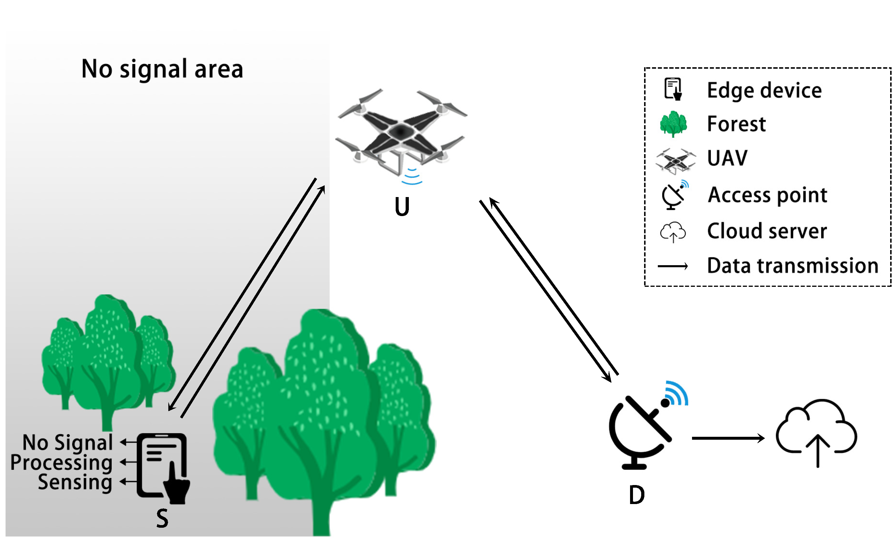
In this paper, we consider a UAV-assisted relay architecture with a two-hop full-duplex transmission scenario in a 3D environment, as shown in Figure 1. The relay system adopts the amplify-and-forward (AF) strategy, which only amplifies the energy of the signal without demodulation and modulation. The system consists of three nodes: ED S and access point D are two ground transceivers, and the overhead base station U is a UAV. In this case, D is fixed in the signal coverage area and can interact with the cloud. S is in the no-signal coverage area due to operational needs. S and D cannot communicate properly due to severe path loss or physical barriers between S and D. U performs irregular movements in the air carrying a mobile base station as a mobile relay to assist in information exchange. We assume that the ED S, the access point D and the overhead base station U are equipped with a transmitter and a receiver, and with two antennas, one for receiving information and one for transmitting it [46]. According to the Cartesian coordinate system, the coordinates of S $U_S$ and D $U_D$ are $\left(x_s,y_s,h_s\right)$$\left(x_d,y_d,h_d\right)$, respectively, and the UAV U performs irregular flight in the no-signal area between the ground transceiver S and D. The instantaneous position $U_t\left(t\right)$ of the UAV U can be expressed as $\left(x\left(t\right),y\left(t\right),h\left(t\right)\right)$. Because the UAV flies at high altitudes with less communication obstruction, the communication is considered as LOS communication in this paper.

Assuming that the emission energy of node S is $P_S$, the upload signal received by the UAV contains both transmission and interference signals. Thus, the signal $Y_{SU}\left(t\right)$ received by the UAV at the predicted node is

$$Y_{SU}\left(t\right)=\sqrt{P_S}{L}_{SU}\left(t\right)X_S\left(t\right)+{\delta }_U\left(t\right)$$

(1)

where $X_S\left(t\right)$ is the instantaneous transmit signal of node S, $L_{SU}\left(t\right)$ is the instantaneous path loss [47] coefficient between S and U, ${\delta }_U\left(t\right)$ is the transmission system noise during the relay transmission from S to U. Its signal-to-noise ratio is ${\gamma }_{SU}=\frac{P_S{\left|L_{SU}\left(t\right)\right|}^2}{{{\delta }_U\left(t\right)}^2}$.

The system uses an AF strategy, so the download energy transmitted by the UAV is the amplified upload signal energy. Then, the download energy $P_{\tau }$ of UAV can be expressed as

$$P_{\tau }=\beta \left(\tau \right)E\left\{{\left|Y_{SU}\left(t\right)\right|}^2\right\}$$

(2)

where $\beta \left(\tau \right)$ is the signal forwarding gain, $\left|Y_{SU}\left(t\right)\right|$ is the amplitude of the signal $Y_{S{U}_a}\left(t\right)$ and $E\left\{·\right\}$ is the expectation of ${\left|Y_{S{U}_a}\left(t\right)\right|}^2$. Therefore, the download signal of the UAV is

$$X_{UD}\left(\tau \right)=\sqrt{\beta \left(\tau \right)}{Y}_{SU}\left(t\right)$$

(3)

The upload signal received by node D is

$$Y_D\left(t\right)=L_{UD}\left(t\right)\sqrt{\beta \left(\tau \right)}{Y}_{SU}\left(t\right)+{\delta }_D\left(t\right)$$

(4)

where $L_{UD}\left(t\right)$ is the instantaneous path loss coefficient between S and U, ${\delta }_D\left(t\right)$ is the transmission system noise in the relay transmission from U to D. Its signal-to-noise ratio is ${\gamma }_{UD}=\frac{P_{\tau }{\left|L_{UD}\left(t\right)\right|}^2}{{{\delta }_D\left(t\right)}^2}$. Then, ${\gamma }_{SD}$ can be expressed as

$$\begin{array}{cc}\hfill {\gamma }_{SD}& =\frac{P_S{\left|L_{SU}\left(t\right)\right|}^2{\beta \left(\tau \right)}^2{\left|L_{UD}\left(t\right)\right|}^2}{{\beta \left(\tau \right)}^2{\left|L_{UD}\left(t\right)\right|}^2{\left|{\delta }_U\left(t\right)\right|}^2+{\left|{\delta }_D\left(t\right)\right|}^2}\hfill \\ \hfill & =\frac{{\gamma }_{SU}{\gamma }_{UD}}{{\gamma }_{SU}+{\gamma }_{UD}+1}\hfill \end{array}$$

(5)

3. Problem Analysis and Optimization

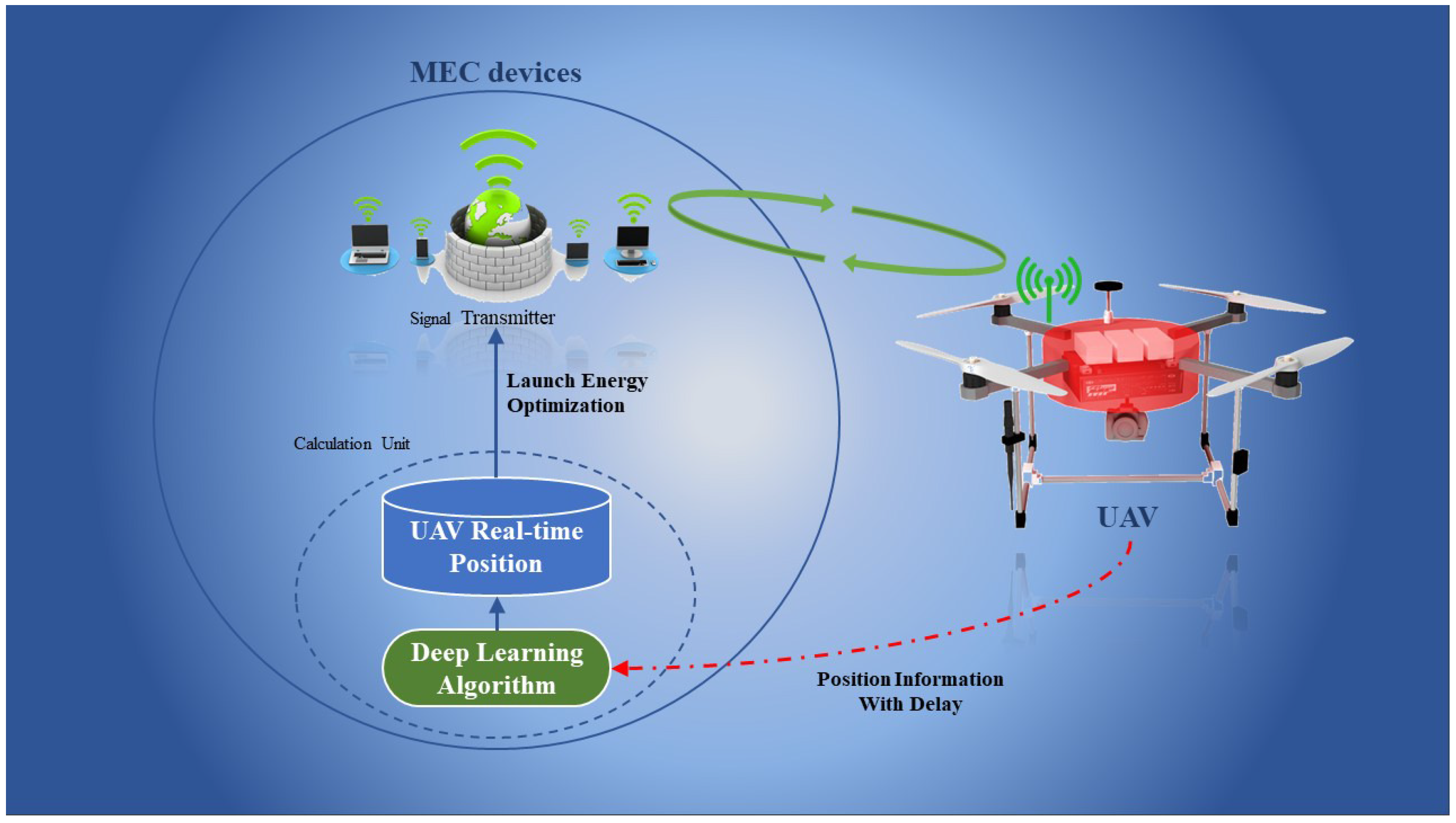
We take into account that EDs need to operate in the field and are required to work for as long as possible without compensating energy. Therefore, a lower energy loss enables EDs to have a longer operating time. The fixed emission energy for data transmission often makes the received signal energy far exceed the receiver sensitivity, resulting in ineffective energy loss. To address this challenge, in what follows, we propose a deep learning-based energy optimization algorithm. The specific implementation framework of the algorithm is shown in Figure 2. First, we formulate the problem to obtain the environmental variables that affect the emission energy under limited conditions. Then, we develop a prediction model using a DL algorithm to address the uncertainty of the environmental variables due to the transmission time delay.

3.1. Problem Formulation

In order to minimize the emission energy of the ED, the emission energy needs to be adaptively adjusted according to the distance between the transmitting end and the receiving end to meet the purpose of transmission and energy saving at the same time. Because the ED end, the UAV end and the ground receiving end are equipped with full-duplex communication devices, the process of communication relay can be regarded as two wireless communication processes. In the single communication process, the system satisfies the free-space propagation model, and the emission energy is expressed as

$$P_S={\left(4\pi \right)}^2{d}^2{P}_{R}L/G_T{G}_R{\lambda }^2$$

(6)

where $G_T$ is the transmit antenna gain, $G_R$ is the receive antenna gain, $\lambda$ is the wavelength and d is the distance between the transmitter and the receiver. L is the system loss factor, which is a constant coefficient dependent on the antenna characteristics and the average channel loss, independent of the transmission. $P_R$ is the received energy, and the value of $P_S$ will be minimum when the value of $P_R$ is equal to the receiver sensitivity $P_{Rmin}$. $P_{Rmin}$ can be expressed as

$$P_{Rmin}=kB\left[T_a+T_e\right]SN{R}_{omin}$$

(7)

where k is Boltzmann constant, B is the system equivalent noise bandwidth, $T_a$ is the antenna noise temperature, $SN{R}_{omin}$ is the demodulator required minimum signal-to-noise ratio. $T_e$ is the equivalent noise temperature, can be expressed as

$$T_e=\left(F_T-1\right)T_0$$

(8)

where $F_T$ is the total equivalent noise figure and $T_0$ is the thermodynamic temperature. Assume that $F_T$ is only related to the gain and noise figure of each monopole of the receiver, then $F_T$ can be expressed as

$$F_T=1+{\displaystyle \sum _{i=1}^n}\frac{(F_i-1)}{{\displaystyle \prod _{j=0}^{i=1}}{G}_j}$$

(9)

In the above formula, $F_i$ is the level i noise figure, $G_j$ is the level i gain, where $G_0$ is 1. It follows that the receiver sensitivity does not change with the environment and $P_{Rmin}$ is a constant. Therefore, the minimum transmit energy $P_{Smin}\left(t\right)$ varies with time t and can be expressed as

$$P_{Smin}\left(t\right)={\left(4\pi \right)}^2{d\left(t\right)}^2{P}_{Rmin}L/G_T{G}_R{\lambda \left(t\right)}^2$$

(10)

From this, we can see that the minimum emission energy is only related to the transmitter transmitting signal wavelength $\lambda \left(t\right)$ and the distance $d\left(t\right)$ between the transmitter and the receiver. Where $\lambda \left(t\right)=u/f\left(t\right)$, u is the speed of light and $f\left(t\right)$ is the real-time emission frequency. To perform adaptive adjustment of the emission energy, the ED receives real-time position information $U_t\left(t\right)$ of the relay UAV through the RF-wireless device and calculates the relative distance $d_{S{U}_t}\left(t\right)$ between the transmitter of the ED and the receiver of the UAV based on its position information $U_s\left(t\right)$. Finally, based on the real-time transmitter frequency ${\lambda }_{SU}\left(t\right)$ and the known spatial noise, receiver sensitivity, transmit antenna gain, receive antenna gain and system loss factor, the required minimum transmitting energy $P_{Smin}\left(t\right)$ is calculated.

3.2. Adaptive Energy Regulation of EDs

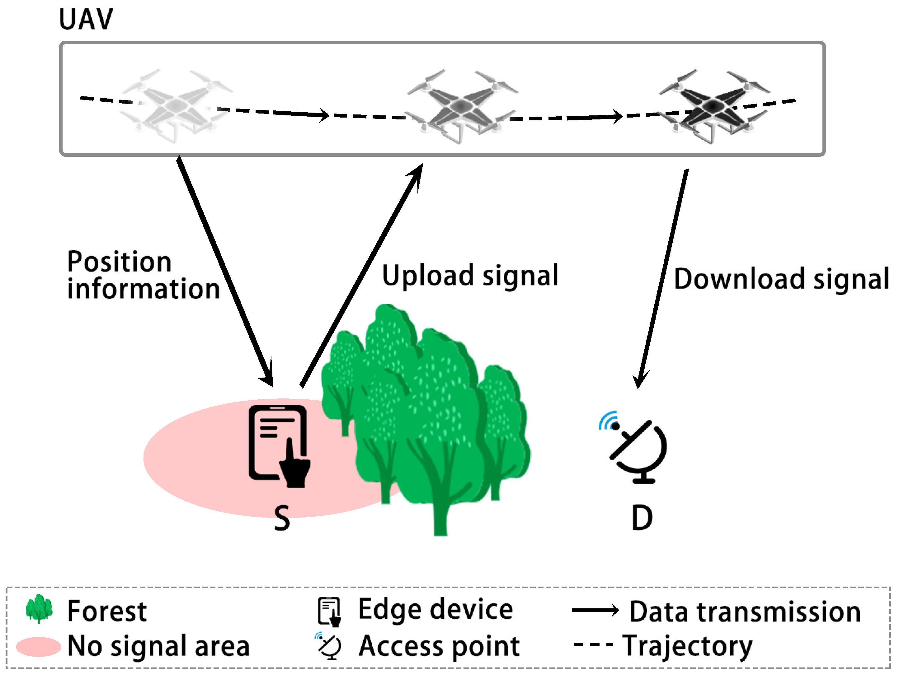
The ED can obtain ${\lambda }_{SU}\left(t\right)$ information in real-time during the process of signal transmission and obtain real-time location information $U_t\left(t\right)$ of the UAV through the wireless device. However, it can be seen from Figure 3 that the real-time position information of the UAV obtained by the ED is lagging due to the communication delay. That is, the relay UAV is not at the coordinates at the time of informing S when loading the information from the edge end. This leads to an incorrect relative distance obtained by the calculation at the ED side, making the emission energy acquisition incorrect. In the system, the equipment carried by S and U is fixed, and the transmitting and receiving antennas are fixed. Therefore, under the condition that the receiver sensitivity is certain and the wavelength is certain, the emission energy is related to the transmission distance of the system. The UAV can obtain real-time spatial position information through global navigation satellite system (GNSS) equipment during the overhead operation. The real-time position distance $d_{S{U}_t}\left(t\right)$ between the UAV and the ED can be expressed as

$$d_{S{U}_t}\left(t\right)=\sqrt{{(x\left(t\right)-x_s)}^2+{(y\left(t\right)-y_s)}^2+{(h\left(t\right)-h_s)}^2}$$

(11)

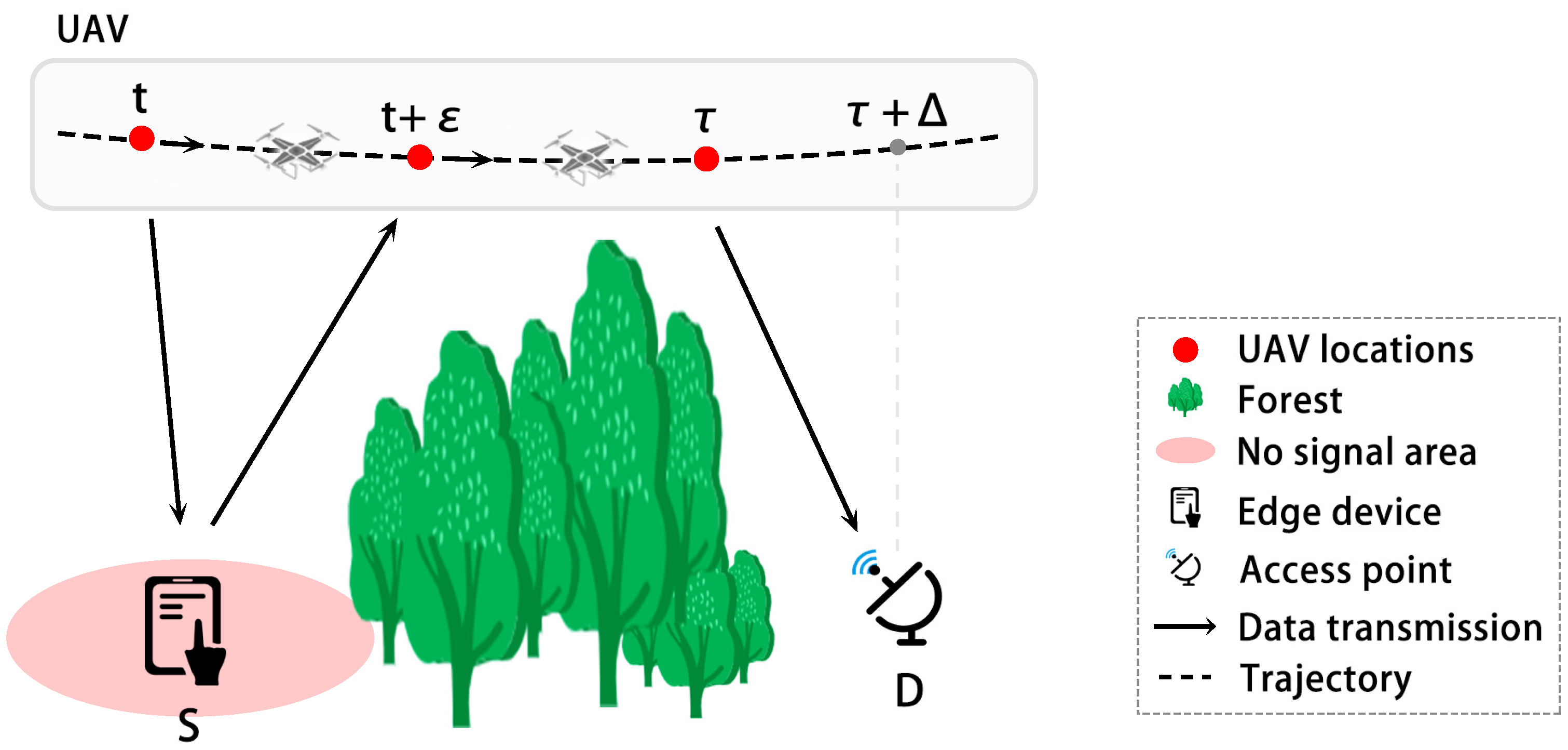
In the communication system, because the UAV performs irregular random motion, the ED obtains the position information of the UAV by transmitting the instantaneous position information of the UAV to the ED through wireless from the UAV side. After the MEC performs the calculation, the ED adjusts the emission energy to send the required relay information to the relay UAV. In this process, communication delay and computation delay are generated, so the UAV position information acquired by the ED is lagged. This can lead to errors in the transmit energy obtained by the computation. In a 6G environment, the communication channel will have a larger bandwidth and lower latency; thus, WD, TD and QD will be negligible compared to PD [36]. As shown in Figure 4, the UAV at t moment sends its position information to S and receives the upload signal in time $t+\epsilon$. After amplification, the UAV sends the download signal to D at $\tau$ time. The time for D to receive the download signal is $\tau +\Delta$. In general, the transmission distance does not vary much, and the PD can be considered as a constant. Therefore, we set the time delay to $\epsilon$, then the actual communication distance between the ED and the UAV when the relay UAVs load data transmitted by the ED can be expressed as

$$d_{SUa}\left(t\right)=\sqrt{{(x(t+\epsilon )-x_s)}^2+{(y(t+\epsilon )-y_s)}^2+{(h(t+\epsilon )-h_s)}^2}$$

(12)

During flight operations, the UAV moves in the air, generally $d_{S{U}_a}\left(t\right)\ne d_{S{U}_t}\left(t\right)$ due to the existence of communication time delay. In order to obtain the correct emission energy of the ED, it is necessary to obtain more accurate real-time position information of the UAV. Specifically, we need to predict the real position of the UAV when the information is loaded based on the historical position information after obtaining the historical real motion trajectory of the UAV. We will predict the actual location information of the UAV through DL and then change the ED emission energy based on the geometric information.

3.2.1. DL

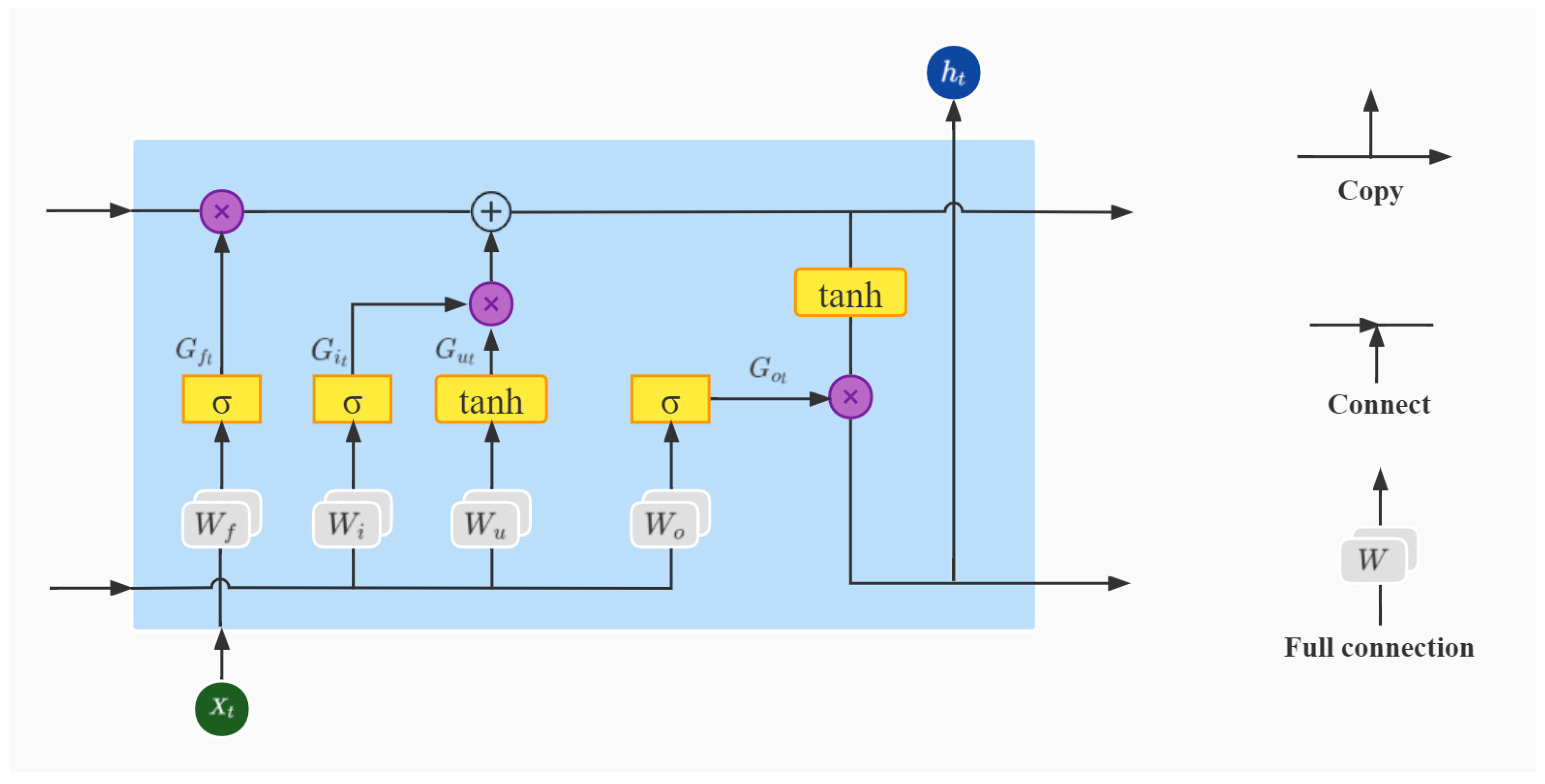
DL can mimic the mechanisms of the human brain to interpret data. In this paper, long short-term memory (LSTM) and its related algorithms are used to predict the trajectory of the UAV. LSTM is a specific type of recurrent neural network (RNN). LSTM differs from RNN in that LSTM can solve gradient exploding problems and learn from long-term dependent information. As shown in Figure 5, an LSTM cell consists of four components: forget gate, input gate, output gate and cell state. The cell of LSTM can be represented by the mathematical formula

$$\left\{\begin{array}{c}{G}_{f_t}=\sigma \left[W_f(h_{t-1},X_t)+b_f\right]\hfill \\ G_{i_t}=\sigma \left[W_i(h_{t-1},X_t)+b_i\right]\hfill \\ G_{\widetilde{c_t}}=\tanh \left[W_{\tilde{c}}(h_{t-1},X_t)+b_{\tilde{c}}\right]\hfill \\ G_{o_t}=\sigma \left[W_o(h_{t-1},X_t)+b_o\right]\hfill \\ C_t=G_{f_t}⨀C_{t-1}+G_{i_t}⨀G_{\widetilde{c_t}}\hfill \\ h_t=G_{o_t}⨀\tanh \left(C_t\right)\hfill \end{array}\right.$$

(13)

where $G_{f_t}$ denotes the forget gate, whose value is restricted between $(0,1)$ by the sigmoid activation function. $W_f$ and $b_f$ denote the weights and biases of the forget gate neurons, respectively. $G_{i_t}$ denotes the input gate, whose value is restricted between $(0,1)$ by the sigmoid activation function, and $W_i$ and $b_i$ denote the weights and biases of the input gate neurons, respectively. $G_{\widetilde{c_t}}$ denotes the candidate cell state, whose value is restricted between $(-1,1)$ by the hyperbolic tangent activation function, and $W_{\tilde{c}}$ and $b_{\tilde{c}}$ denote the weights and biases of the candidate cell state neurons, respectively.

$G_{o_t}$ denotes the output gate, whose value is restricted between $(0,1)$ by the sigmoid activation function, and $W_o$ and $b_o$ denote the weights and biases of the output gate neurons, respectively. $C_t$ denotes the cell state, and ⨀ denotes the product of elements. $h_t$ is the hidden layer state. $X_t$ denotes the input of the neural network at the current moment, and $h_{t-1}$ denotes the state of the hidden layer at the previous moment.

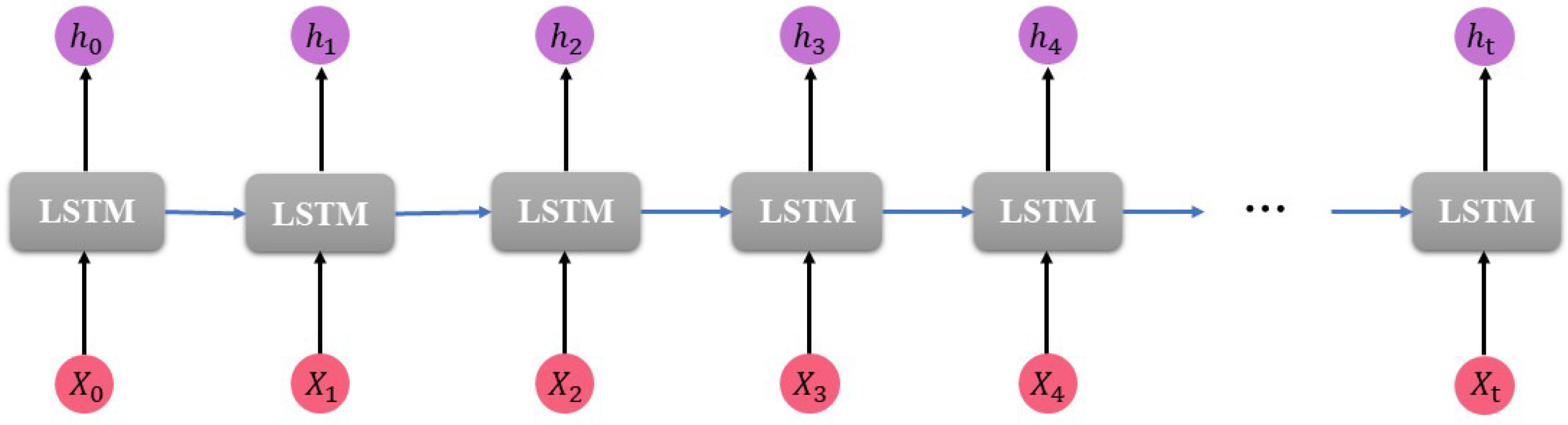
As Figure 6 shows, the LSTM uses cell states $C_t$ and hidden states $h_t$ to obtain information from the history $x_1,\dots ,x_{t-1}$ and the current input $x_t$, and the final hidden state is completely dependent on the previous historical input information. However, in many cases, the current state is not only related to historical information but also future information and can reflect some information about the current state. Bidirectional long short-term memory (Bi-LSTM) solves this problem.

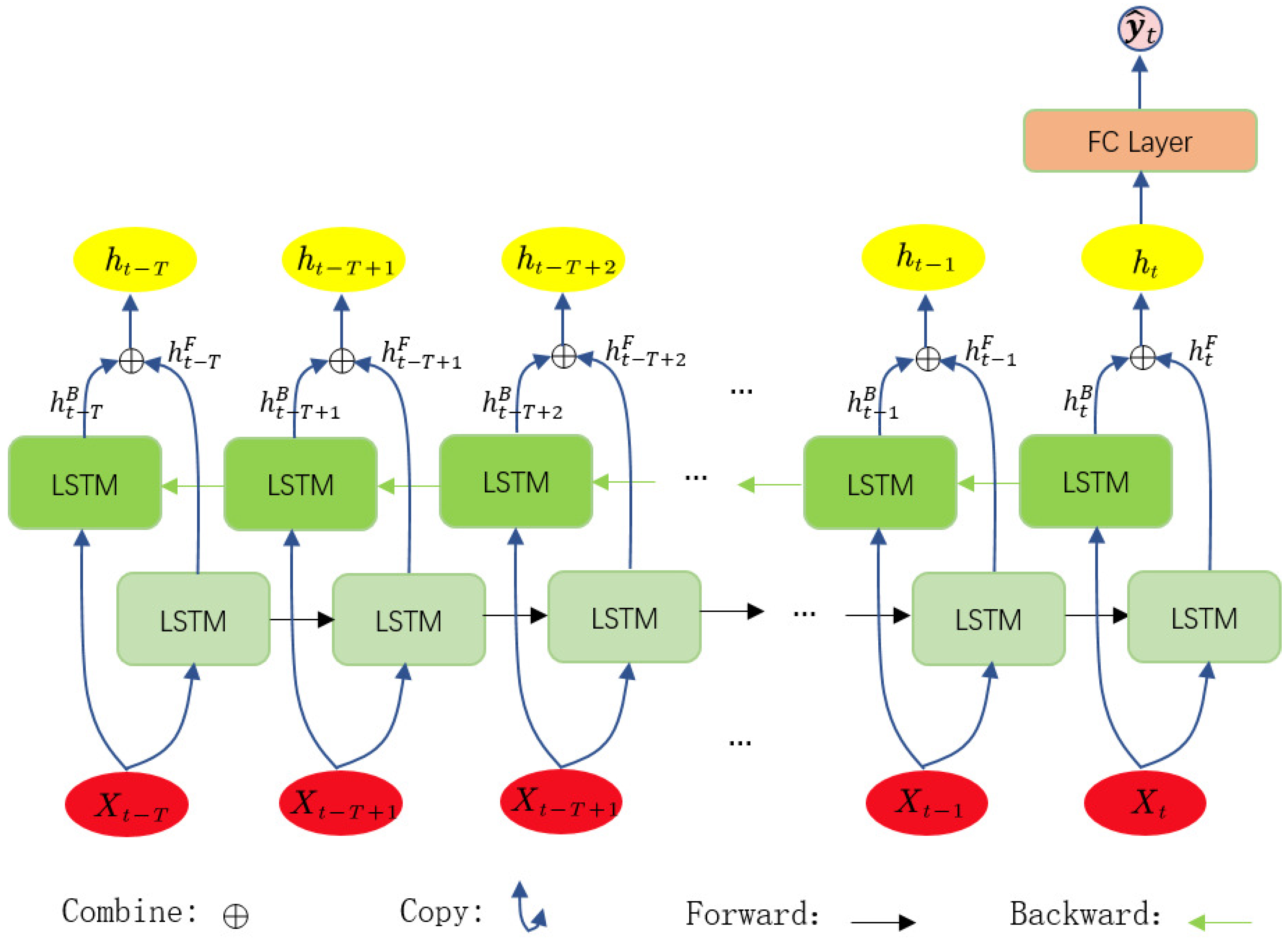
Bi-LSTM can merge the future information $x_{t+1},\dots ,x_T$ near the current input information for model building in order to obtain the current output. As Figure 7 shows, Bi-LSTM can achieve this function by using two separate hidden layers to process the forward data and backward data and then merging them into the same output layer.

In Figure 7, the black arrow points to the forward LSTM branch and the green arrow points to the backward LSTM branch. The data are input into two independent branches, respectively, and the two independent outputs are finally combined into one output. The Bi-LSTM calculates the forward hidden state $h_t^F$, the backward hidden state $h_t^B$ and the final output $h_t$ by Equations (14)–(16).

$$\left\{\begin{array}{c}{G}_{f_t}^F=\sigma \left[W_f^F(h_{t-1}^F,X_t)+b_f^F\right]\hfill \\ G_{i_t}^F=\sigma \left[W_i^F(h_{t-1}^F,X_t)+b_i^F\right]\hfill \\ G_{\widetilde{c_t}}^F=\tanh \left[W_{\tilde{c}}^F(h_{t-1}^F,X_t)+b_{\tilde{c}}^F\right]\hfill \\ G_{o_t}^F=\sigma \left[W_o^F(h_{t-1}^F,X_t)+b_o^F\right]\hfill \\ C_t^F=G_{f_t}^F⨀C_{t-1}^F+G_{i_t}^F⨀G_{\widetilde{c_t}}^F\hfill \\ h_t^F=G_{o_t}^F⨀\tanh \left(C_t^F\right)\hfill \end{array}\right.$$

(14)

$$\left\{\begin{array}{c}{G}_{f_t}^B=\sigma \left[W_f^B(h_{t+1}^B,X_t)+b_f^B\right]\hfill \\ G_{i_t}^B=\sigma \left[W_i^B(h_{t+1}^B,X_t)+b_i^B\right]\hfill \\ G_{\widetilde{c_t}}^B=\tanh \left[W_{\tilde{c}}^B(h_{t+1},X_t)+b_{\tilde{c}}^B\right]\hfill \\ G_{o_t}^B=\sigma \left[W_o^B(h_{t+1}^B,X_t)+b_o^B\right]\hfill \\ C_t^B=G_{f_t}^B⨀C_{t+1}^B+G_{i_t}^B⨀G_{\widetilde{c_t}}^B\hfill \\ h_t^B=G_{o_t}^B⨀\tanh \left(C_t^B\right)\hfill \end{array}\right.$$

(15)

$$h_t=W^F{h}_t^F+W^B{h}_t^B+b_h$$

(16)

Equation (14) is the mathematical expression for the forward branch in the Bi-LSTM model, where the parameters are consistent with the traditional LSTM. Equation (15) is the mathematical expression of the backward branch. The only difference with Equation (14) is that the hidden state which calculates the value of each gate together with the current input $X_t$ is not obtained based on the historical input information $h_{t-1}$ but on the future input information $h_{t+1}$.

Taking the UAV path time-series data $X_T$ with length T as the input of this network, the features extracted through the first layer of bidirectional LSTM network are passed to the next layer of overlay network as the input, loop until the last hidden layer of LSTM of the last layer is used as the input to the fully connected network. The fully connected network predicts and outputs the future position value ${\widehat{y}}_t$ of UAV with one time step, which can be expressed as

$${\widehat{y}}_t=w{h}_T^L$$

(17)

where w is an $n\times m$ matrix, n is the dimensionality of the output features and m is the dimensionality of the hidden layer states. In this way, we can predict the UAV coordinates $U_p$ after the time $\epsilon$ by Bi-LSTM is $(x_p\left(t\right),y_p\left(t\right),h_p\left(t\right))$.

3.2.2. The DEO

We use the position $U_p\left(t\right)$ predicted by DL as the UAV position input system to obtain the UAV and transmitter position relationship.

$$d_{S{U}_p}\left(t\right)=\sqrt{{(x_p\left(t\right)-x_s)}^2+{(y_p\left(t\right)-y_s)}^2+{(h_p\left(t\right)-h_s)}^2}$$

(18)

Then, predict real-time minimum emission energy of the transmitter can be expressed as

$$P_{Smin}\left(t\right)={\left(4\pi \right)}^2{d_{S{U}_p}\left(t\right)}^2{P}_{Rmin}L/G_T{G}_R{\lambda \left(t\right)}^2$$

(19)

The details of this algorithm are summarized in Algorithm 1. To obtain a more approximate adaptive emission energy of the transmitter, we need the following steps: Steps 1–2 select the DL model adapted to the system for the system delay $\epsilon$, train the UAV’s historical flight path and output the UAV’s flight path prediction model based on DL. Steps 4–5 input the real-time UAV position information $U_t\left(t\right)$ received by the transmitter to the prediction model and obtain the predicted position information $U_p\left(t\right)$ of the UAV after the moment $\epsilon$. Steps 6–7 calculate the optimized emission energy $P_{Smin}\left(t\right)$ based on the receiver sensitivity $P_{Rmin}$, spatial noise ${\delta }_R$, transmitter antenna gain $G_T$ and receiver antenna gain $G_R$.

Algorithm 1 The DEO

Require: $U_s$, $U_t\left(t\right)$, $P_{Rmin}$, $\epsilon$, ${\delta }_R$, $G_T$, $G_R$, $t_{max}$; Ensure: $P_{Smin}\left(t\right)$; 1: choose the DL model based on time delay $\epsilon$; 2: train the DL model; 3: while $t<t_{max}$ do 4:    put $U_t\left(t\right)$ into the DL model; 5:    obtain $U_p\left(t\right)$; 6:    calculate $d_{SUp}\left(t\right)$; 7:    calculate $P_{Smin}\left(t\right)$; 8: end while 9: return $P_{Smin}\left(t\right)$;

4. Experiments and Results

In this section, we test the DEO. First, we compare the predicted effect of several DL methods. Then, we test the performance of the algorithm under the effect of different time delays. Finally, we test the practicality of the algorithm in a motion environment.

The parameters of the UAV we use are shown in

Table 1. Parameters of the UAV.

Hardware	Parameter
Flight Controller	Pixhawk
GPS	10 Hz
Maximum speed	1 m/s

. We collect flight data at Fuzhou University, which consists of 12 training sets with a total length of 19,886 points; 4 verification sets, with a total length of 5487 points; and 4 test sets, each with 800 points in length. We use airborne sensors to collect the actual flight data, including the longitude, latitude and altitude of the UAV. We use the Haversine formula [48] to change the coordinates of the UAV from the geographic coordinate system to the Cartesian coordinate system. After removing outliers and averaging and normalizing the data, it is then divided into a training set, a validation set and a test set according to the 3:2:2 division principle. After starting from the starting point, the UAV approaches the end at a variable speed, and it undergoes an altitude change, attitude change and flight angle change on the way, as shown in Figure 8.

In this algorithm, the UAV uses only simpler airborne sensors, such as a GNSS. For these reasons, the following characteristics are defined for the relay UAV:

• Global longitude, which is used to account for the movement of the UAV in the longitude direction.
• Global latitude, which is used to account for the movement of the UAV in the latitude direction.
• Height above ground, the height above ground relative to the altitude of the starting UAV, which is used to account for the movement of the UAV in the direction perpendicular to the ground.

The data from the above three dimensions are transformed into a data set with 3D characteristics in the Cartesian coordinate system. In the experiment, we normalize the data to ensure that the features in each dimension make the same contribution to the results. The processing method is shown below

$${\widehat{x}}_i=\frac{x_i-min}{max-min}$$

(20)

where $x_i$ denotes the ith element in a set of data, $min$ denotes the minimum value in the set, $max$ denotes the maximum value in the set and ${\widehat{x}}_i$ denotes the value of the corresponding element after normalization.

In this paper, we use a PC as the simulation platform. The platform has a CPU of Xeon E5 and a GPU of RTX 3080TI. We implement the design of various LSTM network models required for the experiments on the Keras framework [49]. The output of the model is a regression of the latitude and longitude and altitude of the UAV position, i.e., a prediction of the future position of the UAV at the next moment. Use MEAN, RMSE and WMAPE as the evaluation index of the model:

$$MEAN=\frac{1}{n}\sum _{i=1}^n(y_t-{\widehat{y}}_t)$$

(21)

$$RMSE=\sqrt{\frac{1}{n}\sum _{i=1}^n{(y_t-{\widehat{y}}_t)}^2}$$

(22)

$$WMAPE=\frac{{\sum }_{i=1}^n|y_t-{\widehat{y}}_t|}{{\sum }_{i=1}^n{y}_t}$$

(23)

where $y_t$ denotes the true value, which corresponds to the label value of the training data in this paper, ${\widehat{y}}_t$ denotes the model prediction value, which corresponds to the predicted value given by the model. The network is weight trained by using the mean square error as the loss function, and the smaller the mean square error is, the closer the predicted value of the model is to the true value. In addition, to save training expenses, this paper uses supervised learning for training and uses the Adam optimizer [50] as an optimizer for training the model weights so that the model can converge quickly and accurately.

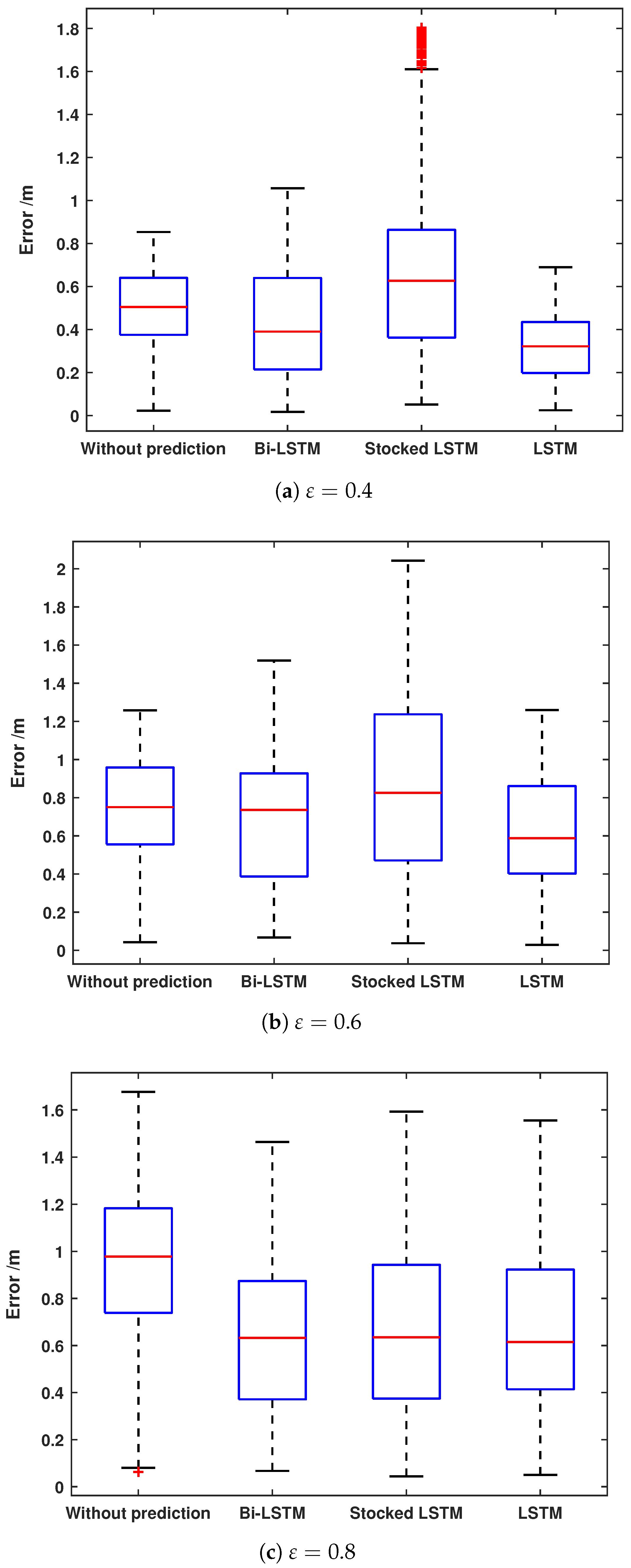
We test the performance of different algorithms under different time delays. The performance results of the no-prediction algorithm, LSTM algorithm, Stacked LSTM algorithm and Bi-LSTM are shown in

Table 2. Performance comparison of path prediction algorithms under different time delays.

		Path 1		Path 2		Path 3		Path 4
Time Delay	Algorithm	MEAN	RMSE	MEAN	RMSE	MEAN	RMSE	MEAN	RMSE
$\epsilon =0.4$	no-prediction	0.4819	0.3019	0.4970	0.3103	0.5105	0.3197	0.5263	0.3284
	LSTM	0.3266	0.2624	0.3132	0.2602	0.3228	0.2713	0.3406	0.2883
	Stacked LSTM	0.6932	0.5103	0.5646	0.4232	0.6148	0.4420	0.7904	0.5988
	Bi-LSTM	0.4407	0.3454	0.4382	0.3239	0.4492	0.3521	0.4185	0.3198
$\epsilon =0.6$	no-prediction	0.7218	0.4513	0.7424	0.4631	0.7637	0.4773	0.7868	0.4899
	LSTM	0.6214	0.5778	0.5693	0.5594	0.5996	0.5780	0.6515	0.6364
	Stacked LSTM	0.8860	0.7675	0.8241	0.7429	0.9067	0.7868	0.8149	0.7396
	Bi-LSTM	0.7003	0.6340	0.6629	0.6232	0.6813	0.6317	0.7600	0.7028
$\epsilon =0.8$	no-prediction	0.9606	0.5993	0.9851	0.6139	1.0143	0.6329	1.0447	0.6490
	LSTM	0.6976	0.6772	0.6630	0.6864	0.6930	0.6887	0.7164	0.7347
	Stacked LSTM	0.6451	0.5656	0.7002	0.5747	0.6992	0.6339	0.7362	0.5658
	Bi-LSTM	0.6282	0.5674	0.5549	0.5512	0.6156	0.5743	0.6243	0.6257

. From the results, it can be seen that the LSTM and Bi-LSTM algorithms achieve a positive effect in the system when the delay $\epsilon >0.4$ s. Their error box diagrams of predicted and true values are shown in Figure 9, and the data are shown in

Table 3. Algorithm error box graph of path 1.

Time Delay	Algorithm	Median	Upper Quarterback	Lower Quarterback
$\epsilon =0.4$	no-prediction	0.50484	0.64050	0.37535
	LSTM	0.32191	0.43489	0.19843
	Stacked LSTM	0.62651	0.86377	0.36274
	Bi-LSTM	0.39045	0.63977	0.21414
$\epsilon =0.6$	no-prediction	0.75086	0.95843	0.55587
	LSTM	0.58762	0.86116	0.40217
	Stacked LSTM	0.82599	1.23710	0.47102
	Bi-LSTM	0.73654	0.92789	0.38704
$\epsilon =0.8$	no-prediction	0.97781	1.18270	0.73878
	LSTM	0.61504	0.99237	0.41395
	Stacked LSTM	0.63471	0.94299	0.37450
	Bi-LSTM	0.63198	087407	0.37119

. In the time of positive effect, LSTM has a better performance when the delay is small. As the delay increases, Bi-LSTM will perform better.

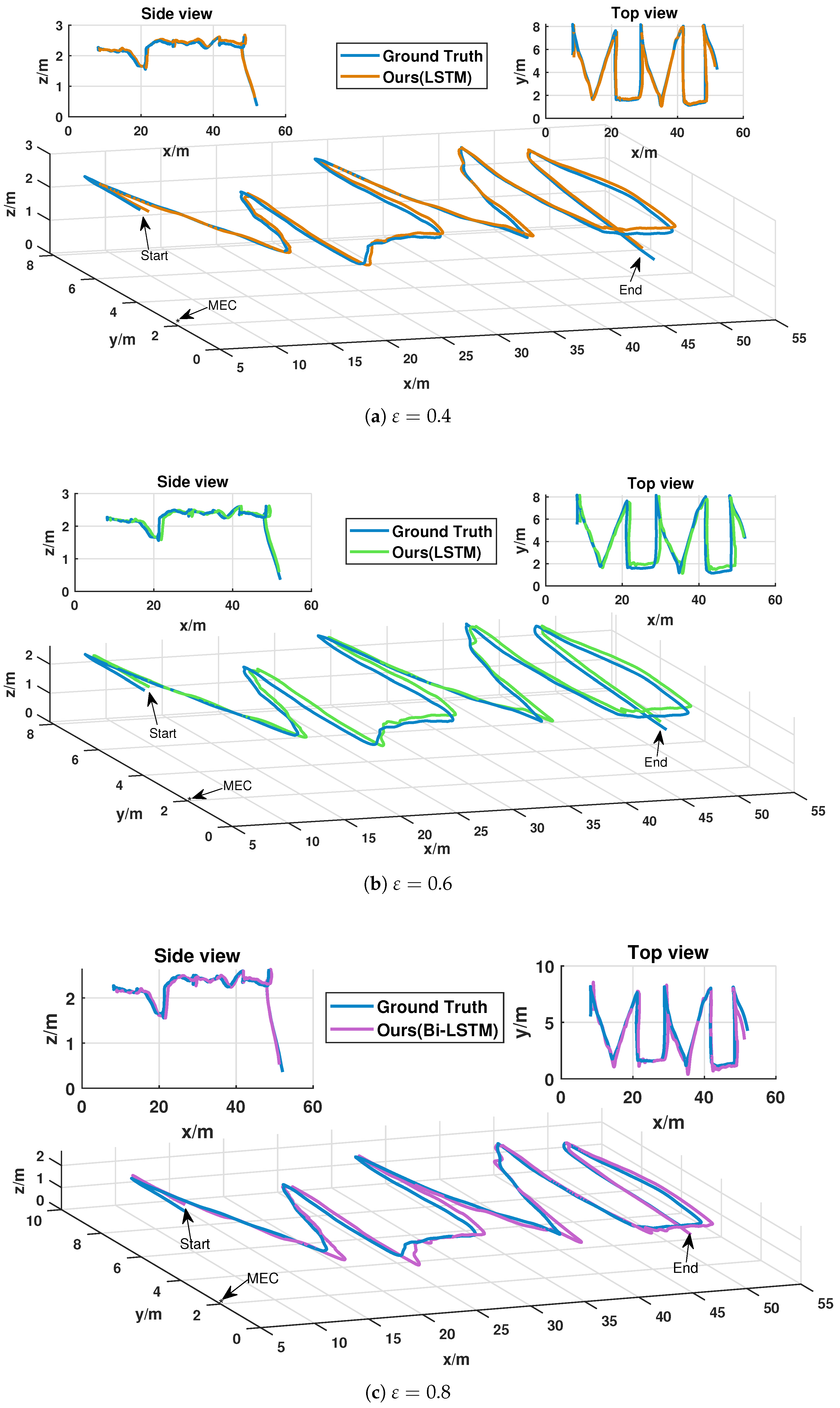
We test the adaptive energy optimization algorithm in simulation. In this case, the data of the UAV are the data from the collection predictions mentioned in this section. The parameters used in the simulation are shown in

Table 4. Simulation parameters.

$f\left(t\right)$	1000 MHz
${\delta }_R$	10 dBm
$G_T$	0
$G_R$	0
Path loss between UAV and ED	$32.45+20\log \left(f\left(t\right)\right)+20\log \left(d_{SUp}\left(t\right)\right)$ [47]
$P_{Rmin}$	−110 dBm
$U_S$	(0,2,0)
The path of the experiment	Path 1

. The DL method we use is selected according to different time delays, as shown in Table 2. The simulation results are shown in Figure 10, Figure 11, Figure 12 and Figure 13.

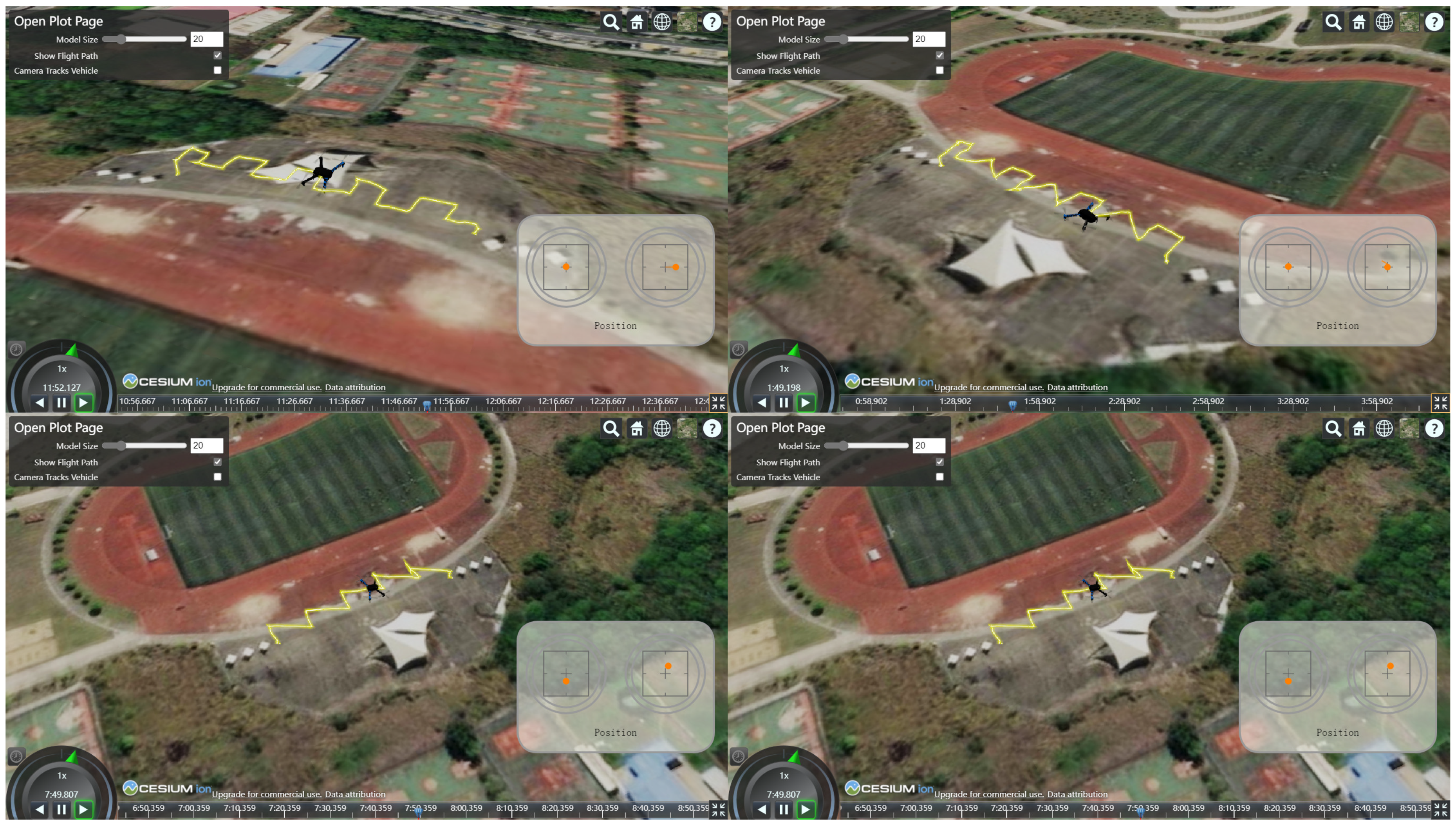
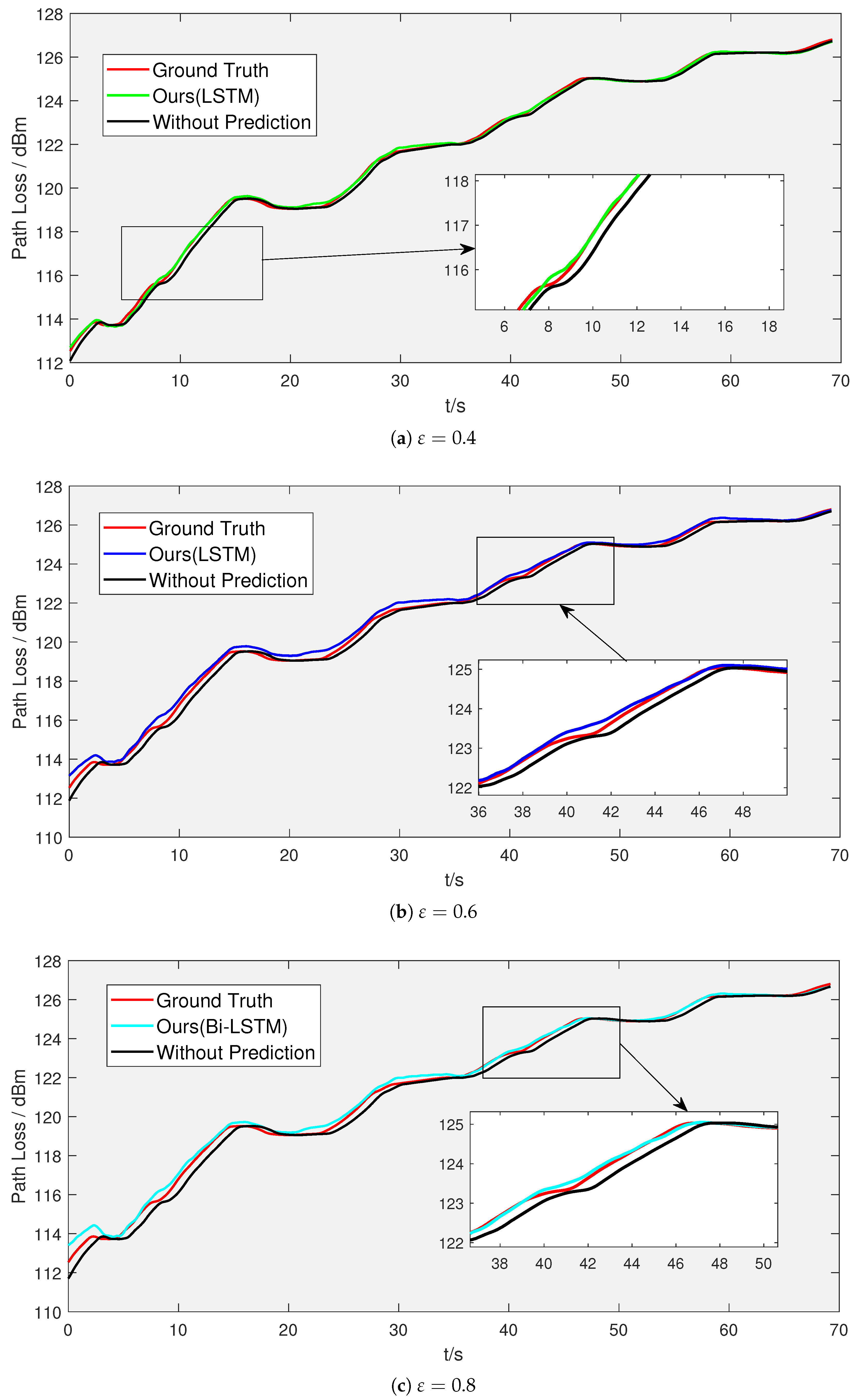
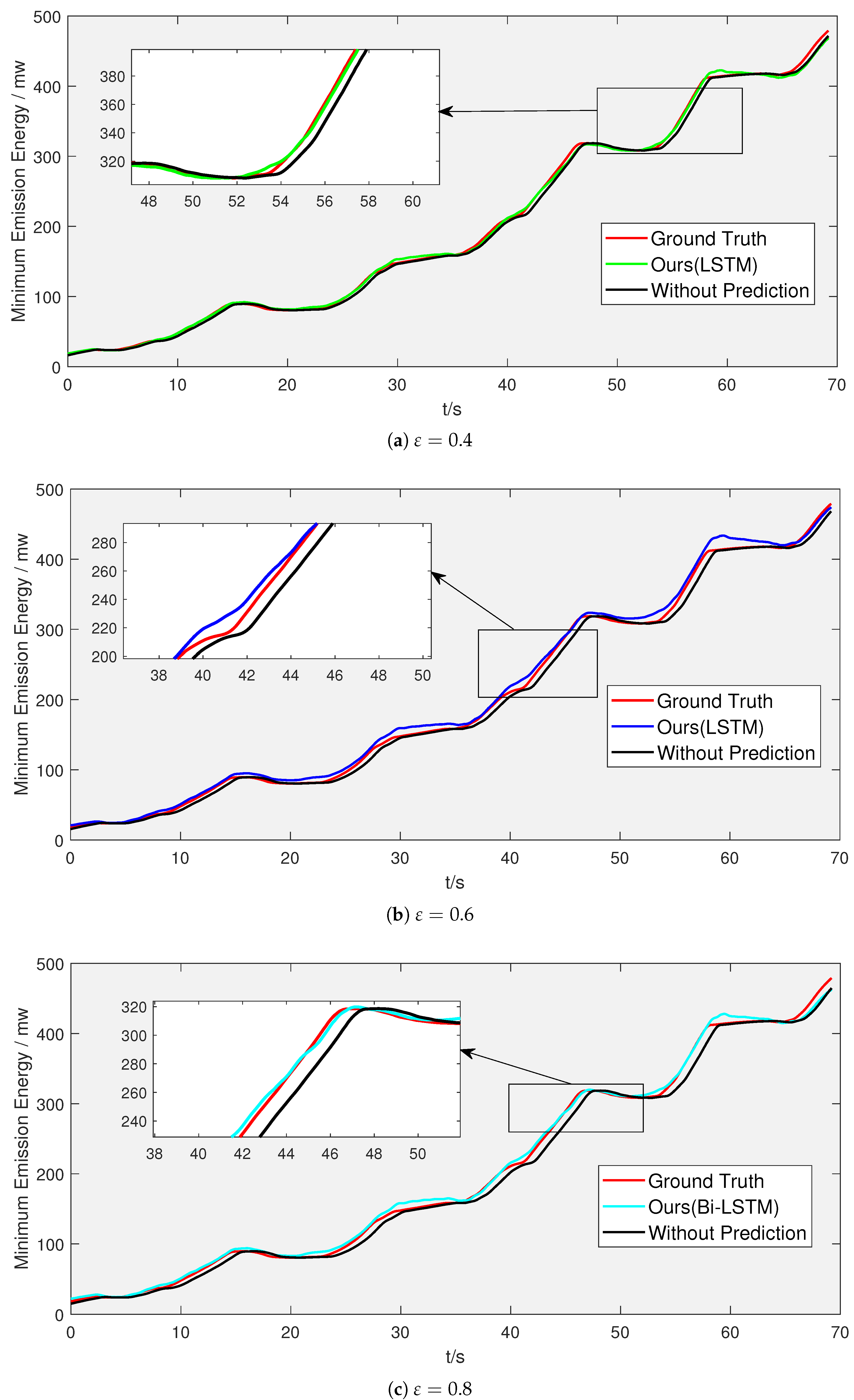
Figure 10 shows the location of the ED and the real trajectory of the UAV flight. Figure 10a–c show the performance of algorithms for the UAV’s flight path prediction under the effect of the time delay of $\epsilon =0.4$, $\epsilon =0.6$ and $\epsilon =0.8$, respectively. Obviously, it can be seen that the algorithm we use is closer to the ground truth and can better describe the actual UAV flight trajectory. It can be seen in Figure 11 and Figure 12 that without the prediction algorithm, the larger the time delay, the larger the error in the calculated path loss and the minimum required emission power, and the system performance crashes as the time delay increases. In contrast, the predictive algorithm can maintain the robustness of the system. Compared with the non-predictive algorithm, our energy optimization method is closer to the true value. Figure 13 shows the minimum received power of the receiver under the action of our algorithm for different time delays.

Table 5. Comparison of $P_S$ performance obtained by calculating at different time delays.

		Path 1			Path 2
Time Delay	Algorithm	MEAN	RMSE	WMAPE	MEAN	RMSE	WMAPE
$\epsilon =0.4$	Prevost et al. [42]	0.1169	0.1803	0.55%	0.1192	0.1895	0.60%
	Shu et al. [45]	0.2634	0.3851	1.24%	0.3302	0.4857	1.64%
	Ours	0.0890	0.1074	0.42%	0.1084	0.1400	0.54%
$\epsilon =0.6$	Prevost et al. [42]	0.1722	0.2644	0.81%	0.1460	0.2259	0.67%
	Shu et al. [45]	0.2521	0.3025	1.19%	0.2267	0.2752	1.04%
	Ours	0.1687	0.2011	0.80%	0.1382	0.1748	0.64%
$\epsilon =0.8$	Prevost et al. [42]	0.2341	0.3589	1.10%	0.2229	0.3535	1.09%
	Shu et al. [45]	0.2167	0.2590	1.02%	0.2447	0.3466	1.20%
	Ours	0.1944	0.2564	0.92%	0.1943	0.3010	0.95%
		Path 3			Path 4
Time Delay	Algorithm	MEAN	RMSE	WMAPE	MEAN	RMSE	WMAPE
$\epsilon =0.4$	Prevost et al. [42]	0.1257	0.1868	0.65%	0.1258	0.1844	0.65%
	Shu et al. [45]	0.3036	0.4460	1.56%	0.3195	0.5157	1.63%
	Ours	0.0993	0.1385	0.52%	0.1049	0.1517	0.54%
$\epsilon =0.6$	Prevost et al. [42]	0.1587	0.2455	0.74%	0.1683	0.2593	0.78%
	Shu et al. [45]	0.2462	0.2865	1.14%	0.2033	0.2485	0.95%
	Ours	0.1430	0.1801	0.66%	0.1614	0.2102	0.75%
$\epsilon =0.8$	Prevost et al. [42]	0.2613	0.3861	1.37%	0.2500	0.3651	1.29%
	Shu et al. [45]	0.2978	0.4502	1.56%	0.2891	0.4494	1.49%
	Ours	0.2053	0.3095	1.08%	0.2231	0.3343	1.15%

shows the algorithm’s performance predictions for $P_S$ under different time-lag systems, and it can be seen that our algorithm outperforms the other algorithms, with better results under the influence of systems with delays greater than 0.4 s. The WMAPE is 0.54%, 0.80% and 1.15% for time delays of 0.4 s, 0.6 s and 0.8 s, respectively. Without the intervention of the prediction algorithm, with the increase in time delay, the difference between the energy obtained by the receiver and the true value is larger, and it cannot be adjusted adaptively. Meanwhile, with the involvement of the prediction algorithm, the energy obtained by the receiver is close to the receiver sensitivity. We can see that the DEO can better optimize the energy output at the transmitter under the condition of guaranteed communication.

5. Conclusions

EDs carry limited energy, and 6G requires a higher transmit energy consumption. In this paper, we study the problem of the emission energy of EDs during UAV relaying. We propose a DEO to adjust the optimal emission power of EDs. Specifically, we use the DL algorithm to predict the path using the historical trajectory characteristics of relay UAVs. Based on the predicted position, the minimum ground emission power that satisfies the receiver sensitivity at the moment the UAV receives the signal under the action of the time-lag system is calculated and obtained to achieve reliable communication between the ED and the relay UAV with the lowest emission energy. We test a variety of DL algorithms in different time-delay systems. The simulation results show that the proposed algorithm can work for time-lag systems with time delays greater than 0.4 s. The WMAPE is 0.54%, 0.80% and 1.15% under the effect of 0.4 s, 0.6 s and 0.8 s time-lag systems, respectively.

However, the method can have some limitations in the face of increasingly complex communication conditions. Therefore, there are still some potential problems that need to be further investigated. We list below some potential research directions in this area.

• The complex environment can interfere with the establishment of communication links. In this paper, we mainly consider UAV communication in an LOS environment. Although the air environment will make the communication environment more friendly, during the mission, UAV communication may be interfered with by many aspects, i.e., multipath effect, occlusion, etc. In this case, the free-space propagation model is not as suitable as the computational model. Therefore, the study of the implemented communication links in complex environments is needed.
• The optimization of computational power in practical fields. Small mobile devices have weak edge computing power and high energy consumption, which makes it difficult to support low-power and long-time work in the field. In short-range UAV emergency communication, the energy used by artificial intelligence to make predictions may be greater than the energy used during communication. Thus, the low-energy algorithm with the precise result is still a challenging task in UAV communications.

References

- Sodhro, A.H.; Pirbhulal, S.; Luo, Z.; Muhammad, K.; Zahid, N.Z. Toward 6G architecture for energy-efficient communication in IoT-enabled smart automation systems. IEEE Internet Things J. 2020, 8, 5141–5148. [Google Scholar] [CrossRef]
- Almalki, F.A.; Soufiene, B.O.; Alsamhi, S.H.; Sakli, H. A low-cost platform for environmental smart farming monitoring system based on IoT and UAVs. Sustainability 2021, 13, 5908. [Google Scholar] [CrossRef]
- Qi, W.; Li, Q.; Song, Q.; Guo, L.; Jamalipour, A. Extensive edge intelligence for future vehicular networks in 6G. IEEE Wirel. Commun. 2021, 28, 128–135. [Google Scholar] [CrossRef]
- Yang, P.; Xiao, Y.; Xiao, M.; Li, S. 6G wireless communications: Vision and potential techniques. IEEE Netw. 2019, 33, 70–75. [Google Scholar] [CrossRef]
- Alsamhi, S.H.; Ma, O.; Ansari, M.S. Artificial intelligence-based techniques for emerging robotics communication: A survey and future perspectives. arXiv 2018, arXiv:1804.09671. [Google Scholar]
- Alsamhi, S.H.; Almalki, F.; Ma, O.; Ansari, M.S.; Lee, B. Predictive estimation of optimal signal strength from drones over IoT frameworks in smart cities. IEEE Trans. Mob. Comput. 2021. [Google Scholar] [CrossRef]
- Zhang, Z.; Xiao, Y.; Ma, Z.; Xiao, M.; Ding, Z.; Lei, X.; Karagiannidis, G.K.; Fan, P. 6G wireless networks: Vision, requirements, architecture, and key technologies. IEEE Veh. Technol. Mag. 2019, 14, 28–41. [Google Scholar] [CrossRef]
- Gao, Y.; Liu, X.; Li, J.; Fang, Z.; Jiang, X.; Huq, K.M.S. LFT-Net: Local Feature Transformer Network for Point Clouds Analysis. IEEE Trans. Intell. Transp. Syst. 2022. [Google Scholar] [CrossRef]
- Yang, H.; Alphones, A.; Xiong, Z.; Niyato, D.; Zhao, J.; Wu, K. Artificial-intelligence-enabled intelligent 6G networks. IEEE Netw. 2020, 34, 272–280. [Google Scholar] [CrossRef]
- Yu, Z.; Gong, Y.; Gong, S.; Guo, Y. Joint task offloading and resource allocation in UAV-enabled mobile edge computing. IEEE Internet Things J. 2020, 7, 3147–3159. [Google Scholar] [CrossRef]
- Huang, M.; Liu, W.; Wang, T.; Liu, A.; Zhang, S. A cloud–MEC collaborative task offloading scheme with service orchestration. IEEE Internet Things J. 2019, 7, 5792–5805. [Google Scholar] [CrossRef]
- Zhang, L.; Ansari, N. Optimizing the operation cost for UAV-aided mobile edge computing. IEEE Trans. Veh. Technol. 2021, 70, 6085–6093. [Google Scholar] [CrossRef]
- Gupta, A.; Sundhan, S.; Gupta, S.K.; Alsamhi, S.H.; Rashid, M. Collaboration of UAV and HetNet for better QoS: A comparative study. Int. J. Veh. Inf. Commun. Syst. 2020, 5, 309–333. [Google Scholar] [CrossRef]
- Chen, C.; Chen, S.; Hu, G.; Chen, B.; Chen, P.; Su, K. An auto-landing strategy based on pan-tilt based visual servoing for unmanned aerial vehicle in GNSS-denied environments. Aerosp. Sci. Technol. 2021, 116, 106891. [Google Scholar] [CrossRef]
- Song, B.D.; Park, K.; Kim, J. Persistent UAV delivery logistics: MILP formulation and efficient heuristic. Comput. Ind. Eng. 2018, 120, 418–428. [Google Scholar] [CrossRef]
- Feng, Q.; Liu, J.; Gong, J. UAV remote sensing for urban vegetation mapping using random forest and texture analysis. Remote Sens. 2015, 7, 1074–1094. [Google Scholar] [CrossRef] [Green Version]
- Faiçal, B.S.; Freitas, H.; Gomes, P.H.; Mano, L.Y.; Pessin, G.; de Carvalho, A.C.; Krishnamachari, B.; Ueyama, J. An adaptive approach for UAV-based pesticide spraying in dynamic environments. Comput. Electron. Agric. 2017, 138, 210–223. [Google Scholar] [CrossRef]
- McRae, J.N.; Gay, C.J.; Nielsen, B.M.; Hunt, A.P. Using an unmanned aircraft system (drone) to conduct a complex high altitude search and rescue operation: A case study. Wilderness Environ. Med. 2019, 30, 287–290. [Google Scholar] [CrossRef] [Green Version]
- Saif, A.; Dimyati, K.B.; Noordin, K.A.B.; Shah, N.S.M.; Alsamhi, S.H.; Abdullah, Q.; Farah, N. Distributed clustering for user devices under unmanned aerial vehicle coverage area during disaster recovery. arXiv 2021, arXiv:2103.07931. [Google Scholar]
- Zhang, S.; Zhang, H.; Song, L. Beyond D2D: Full dimension UAV-to-everything communications in 6G. IEEE Trans. Veh. Technol. 2020, 69, 6592–6602. [Google Scholar] [CrossRef] [Green Version]
- Alsamhi, S.H.; Almalki, F.A.; AL-Dois, H.; Shvetsov, A.V.; Ansari, M.S.; Hawbani, A.; Gupta, S.K.; Lee, B. Multi-Drone Edge Intelligence and SAR Smart Wearable Devices for Emergency Communication. Wirel. Commun. Mob. Comput. 2021, 2021. [Google Scholar] [CrossRef]
- You, C.; Zhang, R. Hybrid offline-online design for UAV-enabled data harvesting in probabilistic LoS channels. IEEE Trans. Wirel. Commun. 2020, 19, 3753–3768. [Google Scholar] [CrossRef] [Green Version]
- Alsamhi, S.H.; Almalki, F.A.; Afghah, F.; Hawbani, A.; Shvetsov, A.V.; Lee, B.; Song, H. Drones’ Edge Intelligence over Smart Environments in B5G: Blockchain and Federated Learning Synergy. IEEE Trans. Green Commun. Netw. 2021, 6, 295–312. [Google Scholar] [CrossRef]
- Chen, P.; Xie, Z.; Fang, Y.; Chen, Z.; Mumtaz, S.; Rodrigues, J.J. Physical-Layer Network Coding: An Efficient Technique for Wireless Communications. IEEE Netw. 2020, 34, 270–276. [Google Scholar] [CrossRef] [Green Version]
- Fang, Y.; Bu, Y.; Chen, P.; Lau, F.C.M.; Otaibi, S.A. Irregular-Mapped Protograph LDPC-Coded Modulation: A Bandwidth-Efficient Solution for 6G-Enabled Mobile Networks. IEEE Trans. Intell. Transp. Syst. 2021. [Google Scholar] [CrossRef]
- Dai, L.; Fang, Y.; Yang, Z.; Chen, P.; Li, Y. Protograph LDPC-Coded BICM-ID With Irregular CSK Mapping in Visible Light Communication Systems. IEEE Trans. Veh. Technol. 2021, 70, 11033–11038. [Google Scholar] [CrossRef]
- Dang, S.; Amin, O.; Shihada, B.; Alouini, M.S. What should 6G be? Nat. Electron. 2020, 3, 20–29. [Google Scholar] [CrossRef] [Green Version]
- Fan, L.; Yan, W.; Chen, X.; Chen, Z.; Shi, Q. An energy efficient design for UAV communication with mobile edge computing. China Commun. 2019, 16, 26–36. [Google Scholar]
- Alzenad, M.; El-Keyi, A.; Lagum, F.; Yanikomeroglu, H. 3-D placement of an unmanned aerial vehicle base station (UAV-BS) for energy-efficient maximal coverage. IEEE Wirel. Commun. Lett. 2017, 6, 434–437. [Google Scholar] [CrossRef] [Green Version]
- Chen, M.; Mozaffari, M.; Saad, W.; Yin, C.; Debbah, M.; Hong, C.S. Caching in the sky: Proactive deployment of cache-enabled unmanned aerial vehicles for optimized quality-of-experience. IEEE J. Sel. Areas Commun. 2017, 35, 1046–1061. [Google Scholar] [CrossRef]
- Yang, Z.; Pan, C.; Wang, K.; Shikh-Bahaei, M. Energy efficient resource allocation in UAV-enabled mobile edge computing networks. IEEE Trans. Wirel. Commun. 2019, 18, 4576–4589. [Google Scholar] [CrossRef]
- Zhang, S.; Zhang, H.; He, Q.; Bian, K.; Song, L. Joint trajectory and power optimization for UAV relay networks. IEEE Commun. Lett. 2017, 22, 161–164. [Google Scholar] [CrossRef]
- Li, M.; Cheng, N.; Gao, J.; Wang, Y.; Zhao, L.; Shen, X. Energy-efficient UAV-assisted mobile edge computing: Resource allocation and trajectory optimization. IEEE Trans. Veh. Technol. 2020, 69, 3424–3438. [Google Scholar] [CrossRef]
- Zhou, F.; Wu, Y.; Hu, R.Q.; Qian, Y. Computation rate maximization in UAV-enabled wireless-powered mobile-edge computing systems. IEEE J. Sel. Areas Commun. 2018, 36, 1927–1941. [Google Scholar] [CrossRef] [Green Version]
- Anand, A.; De Veciana, G.; Shakkottai, S. Joint scheduling of URLLC and eMBB traffic in 5G wireless networks. IEEE/ACM Trans. Netw. 2020, 28, 477–490. [Google Scholar] [CrossRef] [Green Version]
- Zhang, Q.; Chen, J.; Ji, L.; Feng, Z.; Han, Z.; Chen, Z. Response delay optimization in mobile edge computing enabled UAV swarm. IEEE Trans. Veh. Technol. 2020, 69, 3280–3295. [Google Scholar] [CrossRef]
- Ning, Z.; Huang, J.; Wang, X. Vehicular fog computing: Enabling real-time traffic management for smart cities. IEEE Wirel. Commun. 2019, 26, 87–93. [Google Scholar] [CrossRef]
- Ding, Z.; Xu, J.; Dobre, O.A.; Poor, H.V. Joint power and time allocation for NOMA–MEC offloading. IEEE Trans. Veh. Technol. 2019, 68, 6207–6211. [Google Scholar] [CrossRef] [Green Version]
- Kuang, Z.; Li, L.; Gao, J.; Zhao, L.; Liu, A. Partial offloading scheduling and power allocation for mobile edge computing systems. IEEE Internet Things J. 2019, 6, 6774–6785. [Google Scholar] [CrossRef]
- Mozaffari, M.; Kasgari, A.T.Z.; Saad, W.; Bennis, M.; Debbah, M. Beyond 5G with UAVs: Foundations of a 3D wireless cellular network. IEEE Trans. Wirel. Commun. 2018, 18, 357–372. [Google Scholar] [CrossRef] [Green Version]
- Hu, Q.; Cai, Y.; Yu, G.; Qin, Z.; Zhao, M.; Li, G.Y. Joint offloading and trajectory design for UAV-enabled mobile edge computing systems. IEEE Internet Things J. 2018, 6, 1879–1892. [Google Scholar] [CrossRef]
- Prevost, C.G.; Desbiens, A.; Gagnon, E. Extended Kalman filter for state estimation and trajectory prediction of a moving object detected by an unmanned aerial vehicle. In Proceedings of the 2007 American Control Conference, New York, NY, USA, 9–13 July 2007; pp. 1805–1810. [Google Scholar]
- Chen, L.; Chen, P.; Lin, Z. Artificial Intelligence in Education: A Review. IEEE Access 2020, 8, 75264–75278. [Google Scholar] [CrossRef]
- Liu, C.; Yuan, W.; Wei, Z.; Liu, X.; Ng, D.W.K. Location-aware predictive beamforming for UAV communications: A deep learning approach. IEEE Wirel. Commun. Lett. 2020, 10, 668–672. [Google Scholar] [CrossRef]
- Shu, P.; Chen, C.; Chen, B.; Su, K.; Chen, S.; Liu, H.; Huang, F. Trajectory prediction of UAV Based on LSTM. In Proceedings of the 2021 2nd International Conference on Big Data & Artificial Intelligence & Software Engineering (ICBASE), Zhuhai, China, 24–26 September 2021; pp. 448–451. [Google Scholar]
- Alsamhi, S.H.; Rajput, N.S. HAP antenna radiation pattern for providing coverage and service characteristics. In Proceedings of the 2014 International Conference on Advances in Computing, Communications and Informatics (ICACCI), Delhi, India, 24–27 September 2014; pp. 1434–1439. [Google Scholar]
- Friis, H.T. A note on a simple transmission formula. Proc. IRE 1946, 34, 254–256. [Google Scholar] [CrossRef]
- Korn, G.A.; Korn, T.M. Appendix B: B9. Plane and spherical trigonometry: Formulas expressed in terms of the haversine function. In Mathematical Handbook for Scientists and Engineers: Definitions, Theorems, and Formulas for Reference and Review, 3rd ed.; Dover Publications: Mineola, NY, USA, 2000; pp. 892–893. [Google Scholar]
- Ketkar, N. Introduction to keras. In Deep Learning with Python; Apress: Berkeley, CA, USA, 2017; pp. 97–111. [Google Scholar]
- Kingma, D.P.; Ba, J. Adam: A method for stochastic optimization. arXiv 2014, arXiv:1412.6980. [Google Scholar]
Figure 1.
UAV-aided wireless network system.
Figure 2.
Implementation framework of DEO.
Figure 3.
UAV locations in different times.
Figure 4.
UAV working time chart.
Figure 5.
Unit structure of LSTM.
Figure 6.
Expansion diagram of LSTM.
Figure 7.
Expansion diagram of Bi-LSTM.
Figure 8.
Path 3D diagrams for testing the data set.
Figure 9.
Error box diagram of path 1.
Figure 10.
Performance of DEO path prediction under different time delays.
Figure 11.
Path loss using DEO under different time delays.
Figure 12.
Adaptive emission power using DEO under different time delays.
Figure 13.
Energy received by the UAV using DEO under different time delays.