A Hybrid Model and Data-Driven Vision-Based Framework for the Detection, Tracking and Surveillance of Dynamic Coastlines Using a Multirotor UAV

Abstract

A hybrid model-based and data-driven framework is proposed in this paper for autonomous coastline surveillance using an unmanned aerial vehicle. The proposed approach comprises three individual neural network-assisted modules that work together to estimate the state of the target (i.e., shoreline) to contribute to its identification and tracking. The shoreline is first detected through image segmentation using a Convolutional Neural Network. The part of the segmented image that includes the detected shoreline is then fed into a CNN real-time optical flow estimator. The position of pixels belonging to the detected shoreline, as well as the initial approximation of the shoreline motion, are incorporated into a neural network-aided Extended Kalman Filter that learns from data and can provide on-line motion estimation of the shoreline (i.e., position and velocity in the presence of waves) using the system and measurement models with partial knowledge. Finally, the estimated feedback is provided to a Partitioned Visual Servo tracking controller for autonomous multirotor navigation along the coast, ensuring that the latter will always remain inside the onboard camera field of view. A series of outdoor comparative studies using an octocopter flying along the shoreline in various weather and beach settings demonstrate the effectiveness of the suggested architecture.

1. Introduction

1.1. Related Literature

The practical applications of Unmanned Aerial Vehicles (UAVs) have now acquired a wide range from classic photography to surveillance of buildings, areas, or even coastlines. Multirotors have the flexibility to regulate velocity during the flight, maintain their position, recognize and follow targets and dynamically change course if necessary, in both indoor and outdoor settings. Their mechanical simplicity and low cost make them a favored option when speed and precision are critical. In addition, recent advances in navigation and perception sensors have significantly boosted their flying endurance and payload capacity, making them viable platforms for missions such as area coverage and surveillance.

Practicing coastal engineers, managers, and academics now have access to off-the-shelf survey-grade UAV equipment, data processing, and analysis tools. Border surveillance and search and rescue missions are just a few of the many uses of a UAV for coastal surveillance [1,2]. In many of these situations, flying at high altitudes and following a simple GPS-aided track may be sufficient for roughly guiding the vehicle down the shoreline and capturing an image or video data for additional processing. On the other hand, some surveillance applications necessitate a higher level of image detail, resulting in lower altitude flights and precise navigation above the coastline. This performance dictates the incorporation of vision data efficiently (e.g., features, contours, etc.) in the motion control loop, resulting in a variety of task-specific visual servoing schemes.

Litter identification and localization are classic examples of such cases. The concentration of significant volumes of rubbish along coasts is expected, especially during the summer tourist season [3,4,5]. Low altitude UAV flights may offer useful visual information during a litter detection operation regarding the location and classification of the garbage along the shoreline [6]. Human detection in search and rescue missions along the sea, lake, or river shorelines, coastline erosion assessment, particularly in rocky water environments, and water sampling missions in case of environmental disasters. In these cases, the first responder’s access is hazardous or impossible and are all examples that require detailed visual information and UAV servoing at low altitudes (e.g., water sampling in contaminated marine areas).

The basic vision-aided control approaches that appear in the literature are Image-based (IBVS), Position-based (PBVS), 2-$1/2$-D, and Direct visual servoing [7,8,9,10,11]. An error signal is measured on the image plane and routed directly to velocity commands in IBVS control. PBVS systems, on the other hand, utilise retrieved features to generate a (partial) 3-D reconstruction of the environment, [7,8]. The error is calculated in the image plane and is then employed by the control system. Because of the inadequacies of PBVS systems, IBVS techniques have grown in popularity. Any mistakes in the vision system’s calibration will result in faults in the 3-D reconstruction, which will lead to errors during task execution. Furthermore, because the PBVS control law is specified in the 3-D workspace, there is no mechanism for directly regulating the image. As a result, items of interest (including features used by the visual servo system) may escape the camera’s FoV [9].

According to those mentioned above, the use of image-based control in UAV stabilization and tracking control has proven to be highly useful in various applications [12]. In stabilization processes, IBVS has been employed in multiple ways offering different solutions and successful results. Examples are schemes such as decoupling the translational and rotational mathematical equations of a robot’s motion [13,14] and implementation of control schemes using stereo vision camera systems [15]. In addition, studies combining IBVS with LQ-servo methodologies [16], as well as the formulation of adaptive IBVS schemes [17] for the flight of a UAV, are also presented in the literature. IBVS has also been extended to the field of study where it is combined with reinforcement learning methods [18,19].

Regarding target tracking during UAV flights executing IBVS control, various approaches have been presented in the literature. Indicatively there are studies such as, vertical take-off and landing of a UAV while compensating the ground effect through an adaptive sliding mode controller [20], tracking of a moving ground vehicle which executes a predetermined performance control concept while adhering to FoV constraints [21], a discrete-time non-linear model predictive controller (MPC) that solves a computationally intensive restricted optimization problem online to successfully land a quadrotor on a moving and sloped platform [22], use of a linear observer estimating the velocity of the visual features [23], design of an IBVS control method which takes into account the image dynamics uncertainties linked to depth information and target motion, as well as the uncertainty of the robot dynamics [24] and design and deployment of a complete vision-based target tracking and following system with a Deep Neural Network as the scheme’s backbone [25,26]. In the systems mentioned above that consider image-based control for target tracking, the target’s motion is specified by either a low or constant velocity profile.

Visual servo control applications for UAVs in activities linked to surveillance of coastlines or places with similar geomorphological characteristics are particularly limited in the existing literature. The authors of [27] presented the steering of a tiny fixed-wing aircraft throughout the limits of diverse terrains or regions of interest controlled by an autonomous vision-based system. Furthermore, [28] recommended generating a tangent on a recognized shoreline trajectory while integrating image processing directly with the controller. Finally, in [29] a guiding algorithm based on recognizing and extracting geographical tracks from real-time aerial photos, such as rivers, coasts, and highways, was implemented.

It should be noted, however, that IBVS also have significant drawbacks. The control law for an IBVS system entails mapping the image space velocities to robot workspace velocities, a procedure encoded through the image Jacobian. Control issues arise regarding singularities or poor conditioning of the Jacobian, which occur as a relative position and motion of the camera and under-view item function. Furthermore, because the control is executed concerning the image, there is no direct control over the system’s cartesian velocities. Inductively, successful trajectories in the image plane can be transformed into bizarre (and maybe dangerous) trajectories for the vehicle in the Cartesian space [10].

Decoupling translational and rotational degrees of freedom is a regular occurrence in visual servoing tasks in underactuated systems (i.e., UAVs). To overcome the issues with the popular IBVS method, the Partitioned Visual Servo (PVS) control strategy [30] was proposed, is based on decoupled techniques, and has comparable decoupling properties but only uses image plane features. The central concept is to decouple the z axis motion from the other degrees of freedom and create separate controllers for this Degree of Freedom (DoF). Nevertheless, even with the most modern methods of visual servoing for target tracking, there is still the problem of online estimation of target motion, which is not addressed in any of the studies as mentioned above [8].

Estimating the hidden state of a dynamical system from noisy observations in real-time is one of the most fundamental tasks in signal processing and control, having localization, tracking, and navigation applications. The Kalman Filter (KF) soon became the workhorse of state estimation in discrete-time systems that state-space models well describe, thanks to its low-complexity implementation and solid theoretical background [31], while the original KF assumed linear state-space models, many problems encountered in practice are driven by non-linear dynamical equations. As a result, non-linear variations of the original KF, such as the Extended Kalman filter (EKF), were developed soon after its publication, where analytical system and measurement models are considered during filter design [32].

Deep neural networks have seen much success in real-world applications in recent years. It has been proven that these data-driven parametric models may capture the properties of complex processes without the need for explicit (e.g., state-space) models [33,34,35,36,37]. Dosovitskiy et al. presented end-to-end optical flow estimates with convolutional networks in [38]. The flow field output of this model, named FlowNet, takes two images as input. Convolutional networks frequently yield noisy or fuzzy outputs when trained for per-pixel prediction tasks. Network predictions can be subjected to out-of-the-box optimization as a post-processing step as a workaround. For motion segmentation, the original FlowNet was ineffective. FlowNet2 [39], on the other hand, is equally accurate as other state-of-the-art approaches while being orders of magnitude faster. This particular CNN is trained in many different datasets, so it can efficiently deal with optical flow estimation in a case such as a coastline. However, it is evident that data-driven approaches like the one above, even for primary sequences, necessitate many trainable parameters and large data sets and so lack the interpretability of model-based methods.

The shortcomings and advantages of model-based Extended Kalman filtering and data-driven state estimation motivate the employment of a hybrid technique that takes advantage of the best of both worlds: the standard EKF’s soundness and low complexity, as well as DNNs’ model-agnostic nature. As a result, in this work, we exploited a framework called KalmanNet [40] that proposes a hybrid MB/DD online recursive filter. The noise statistics are considered unknown in KalmanNet, and the underlying state-space model is either known or approximated from a physical system dynamics model. The Kalman Gain (KG) computations in the EKF are a significant component encapsulating the dependence on noise statistics and domain knowledge. They are replaced with a simple Recurrent Neural Network (RNN) integrated into the EKF architecture. The resulting system learns to perform Kalman filtering in a supervised manner using labeled data.

1.2. Contributions

In this work, we propose a hybrid MB/DD vision-based framework for the efficient detection and tracking of coastlines in dynamic motion induced by waves, using an autonomous octocopter. The major contributions of this work can be summarized as follows:

• Implementation and training of a CNN for detecting shoreline features from raw camera images.
• Deployment of a CNN for the optical flow estimation of the detected coastline.
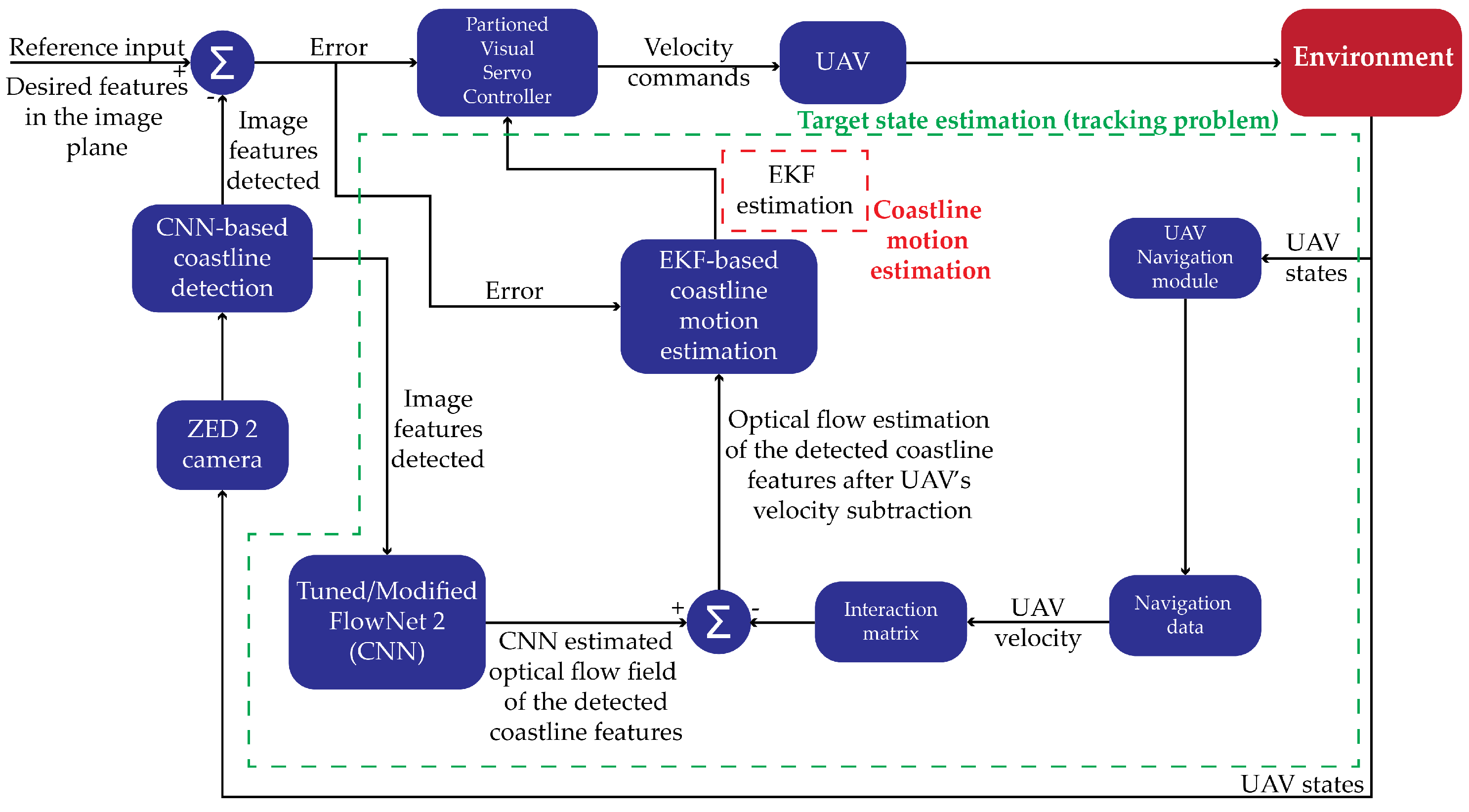
• Formulation of an EKF based on an approximate wave motion model, which provides an online estimate of the coastline motion in the image plane.
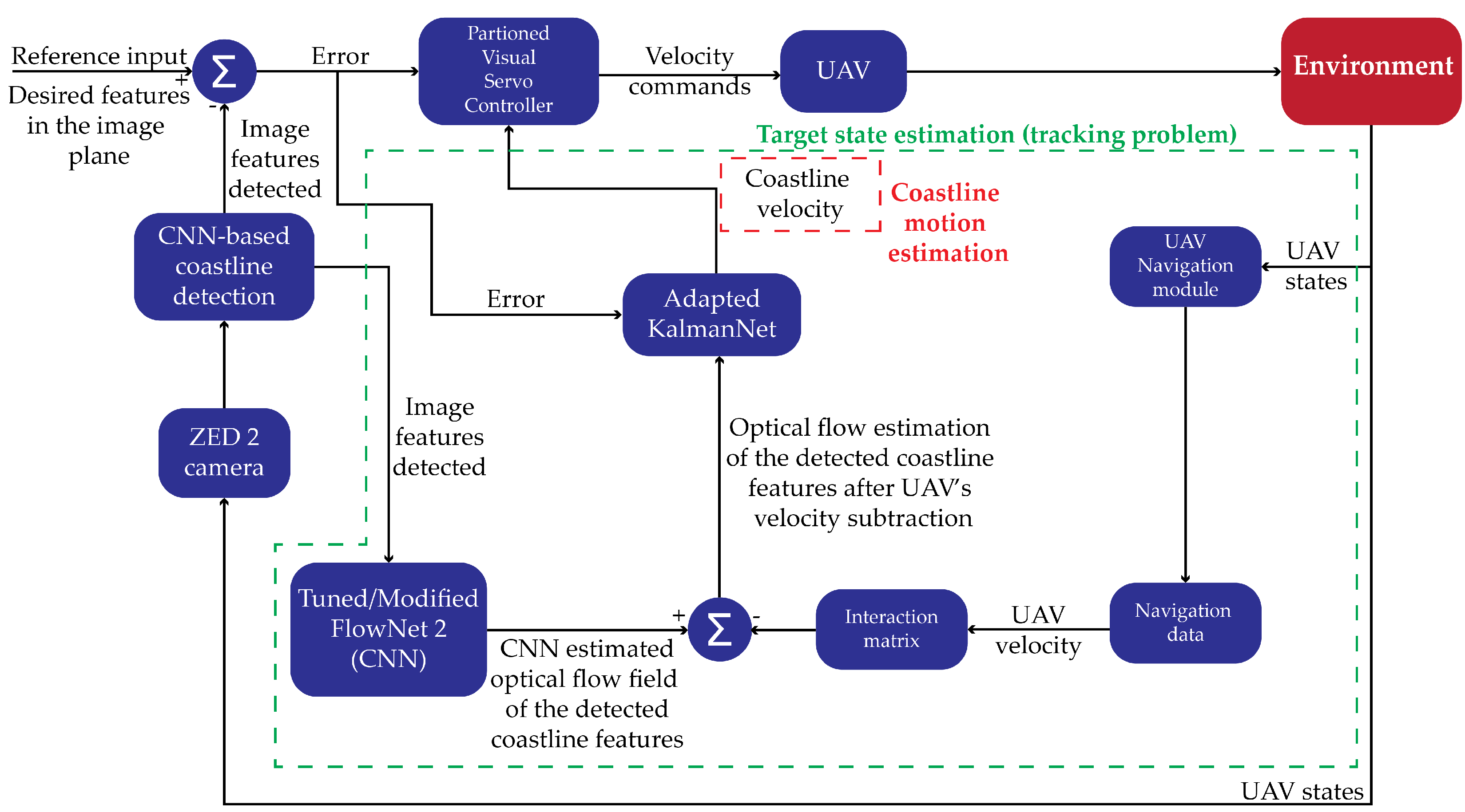
• Formulation of a Neural-Network aided EKF that learns from data. This module combines the EKF implementation (model-based method) and the CNN-based (data-driven method) optical flow estimation to estimate the shoreline motion in the image plane online directly.
• Development of a robust PVS control strategy for the autonomous navigation of an octocopter along a wavy shoreline, incorporating as feedback the output of (4) while ensuring the latter is always retained inside the camera field of view.

1.3. Outline

The remainder of the paper is laid out as follows: Section 2 gives some background on the UAV motion model and low-level control. A description of the problem is presented in Section 3. The methodology applied to synthesize the proposed framework is detailed in Section 4. Section 5 proves the framework’s efficacy through a series of comparative experimental cases. Finally, Section 6 presents the conclusions of this study.

2. Preliminaries

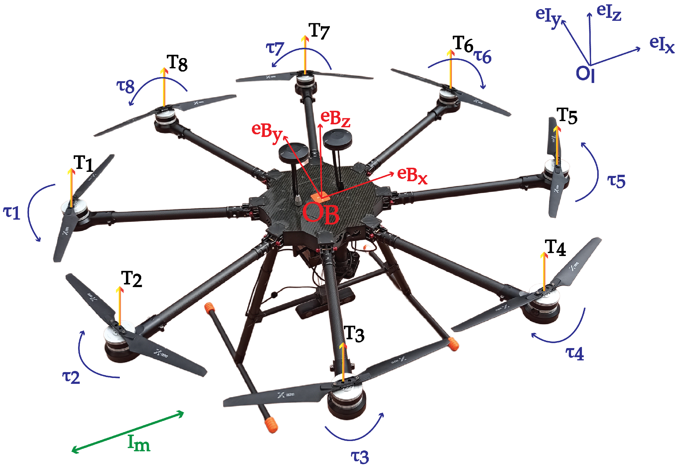
2.1. Multirotor Equations of Motion

The vehicle, depicted in Figure 1, used in this study is a custom-made octocopter comprised of eight fixed-pitch propellers and individual rotors attached to a rigid cross frame. Each rotor produces a thrust that causes roll, pitch, yaw, and overall thrust. The vehicle is controlled via the differential regulation of the thrust. As a result, the thrust and torque applied by each individual motor-propeller set determine the system dynamics [41,42].

A body-fixed frame $\mathbf{B}=\{e_{B_x},e_{B_y},e_{B_z}\}$ is attached to the vehicle’s center of gravity $O_B$, and an inertial frame $\mathbf{I}=\{e_{I_x},e_{I_y},e_{I_z}\}$ is placed at a fixed position $O_I$. The dynamic model of a multirotor can be provided from the general Newton–Euler motion equations of a 6-DoF rigid body subject to external forces and torques, according to [41]:

$$\begin{array}{c}\hfill {}^I{\dot{\mathbf{p}}}_B={}^I{\mathbf{v}}_B\end{array}$$

(1)

$$\begin{array}{c}\hfill m_i{}^I{\dot{\mathbf{v}}\mathbf{s}.}_B={}^I{\mathbf{R}}_B{\mathbf{f}}_B\end{array}$$

(2)

$$\begin{array}{c}\hfill {\mathbf{J}}_B{\dot{\omega }}_B={\mathbf{\tau }}_B\end{array}$$

(3)

where ${}^I{\mathbf{p}}_B={\left[\begin{array}{ccc}{}^I{x}_B& {}^I{y}_B& {}^I{z}_B\end{array}\right]}^T$, the position vector and ${}^I{\mathbf{v}}_B={\left[\begin{array}{ccc}{}^I{v}_{x_B}& {}^I{v}_{y_B}& {}^I{v}_{z_B}\end{array}\right]}^T$ the linear velocity vector of the vehicle wrt the inertial frame $\mathbf{I}$. The angular velocity expressed in $\mathbf{B}$ is given by ${\omega }_B={\left[\begin{array}{ccc}{p}_B& q_B& r_B\end{array}\right]}^T$. The rotation matrix from frame $\mathbf{B}$ to $\mathbf{I}$ is denoted as ${}^I{\mathbf{R}}_B$, ${\mathbf{J}}_{{}_B}$ is the inertia matrix expressed in $\mathbf{B}$ and m is the mass. The definition of the generalized forces and torques applied on the multirotor is presented as follows:

$$\begin{array}{c}\hfill {\mathbf{f}}_B={\mathbf{f}}_M+{\mathbf{f}}_d+{\mathbf{f}}_g\end{array}$$

(4)

$$\begin{array}{c}\hfill {\mathbf{\tau }}_B={\mathbf{\tau }}_M+{\mathbf{\tau }}_d\end{array}$$

(5)

where ${\mathbf{f}}_d$ denotes the drag forces, ${\mathbf{\tau }}_d$ the drag moments, ${\mathbf{f}}_g$ is the gravity vector, ${\mathbf{f}}_M$ and ${\mathbf{\tau }}_M$ are the motor thrust and torque vectors, respectively. More details can be found in [41,42].

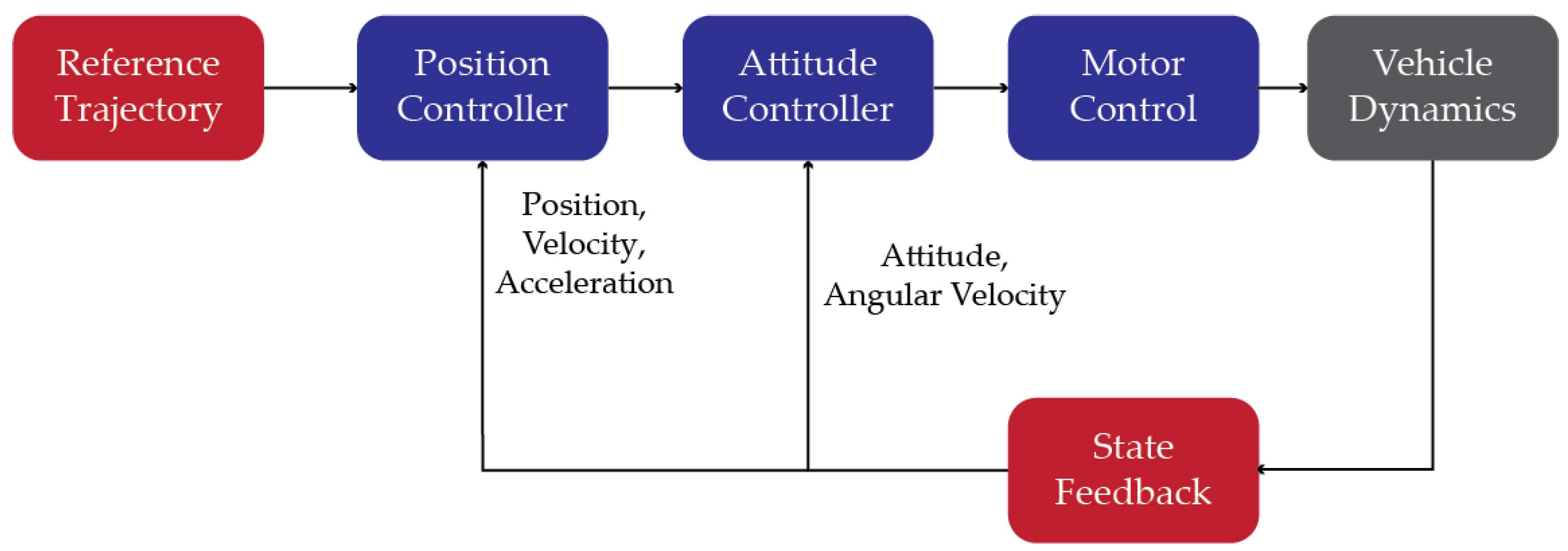
2.2. Multirotor Low-Level Control

The octocopter vehicle used in this study utilizes a Pixhawk Cube Orange [43] featuring the ArduPilot firmware [44]. The complete functionality of the low-level control architecture is implemented as a collection of cascaded P/PID controllers that handle the vehicle’s low-level control via the inner and outer loop architecture as follows:

• an inner loop executing attitude control while using as input references roll, pitch, yaw, and throttle values,
• an outer loop executing translational motion control while using as input references the desired position or velocity values.

This architecture provides for separate control of each axis for minor deviations from the hovering condition. The low-level controller’s outer-loop accepts reference linear velocities and yaw rate in the body-fixed frame $\mathbf{B}$. The commanded torques and vertical thrust are the low-level controller’s outputs, which are finally translated to motor voltages.

Remark 1.

The PVS controller in the proposed method calculates velocities in the camera frame $\mathbf{C}$, which are then converted into the vehicle body frame $\mathbf{B}$ and used as a reference in the low-level controller’s outer loop. An overview of the control architecture is shown in Figure 2.

3. Problem Statement

According to the introductory presentation of the proposed method we begin our study by defining the problem being addressed. We use an octorotor equipped with a downward-looking camera to investigate the PVS tracking problem as part of autonomous coastline monitoring in the presence of coastal waves (Figure 3). The downward-looking camera (Figure 4) is first given a central projection perspective model, which is a common assumption in visual servoing tasks [9]. The camera’s frame is designated by the letter $\mathbf{C}$ with the axes ${[X_c,Y_c,Z_c]}^T$ linked to the center $O_C$. The image frame’s ${\mathbf{I}}_{im}$ coordinates ${[u,v]}^T$ are measured in pixel units and $O_{I_{im}}$ is the picture’s upper-left corner. Using the camera geometrical model, a set of n fixed 3-D points with coordinates ${\mathbf{P}}_{\mathbf{i}}={[X_i,Y_i,Z_i]}^T$, $i=1,\dots ,n$ expressed in the camera frame are projected to the normalized image plane as 2-D points with coordinates ${\mathbf{s}}_{\mathbf{i}}={[x_i,y_i]}^T$, $i=1,\dots ,n$, as follows [9]:

$${\mathbf{s}}_{\mathbf{i}}={\left[\begin{array}{cc}{x}_i& y_i\end{array}\right]}^T={\left[\begin{array}{cc}\frac{u_i-c_u}{{\alpha }_x}& \frac{v_i-c_v}{{\alpha }_y}\end{array}\right]}^T$$

(6)

where $u_i,v_i$ are the pixel coordinates of the i-th feature, $c_u,c_v$ are the pixel coordinates of the primary point, and ${\alpha }_x,{\alpha }_y$ are the pixel focal length for each image axis. If we examine a moving target (i.e., coastline waves), the differential equation that describes the flow of features belonging to the coastline:

$$\begin{array}{c}\hfill \dot{\mathbf{s}}=\mathbf{L}(\mathbf{Z},\mathbf{s}){\mathbf{v}}_c+\frac{\partial \mathbf{s}}{\partial \mathbf{t}}=\\ \hfill {\mathbf{L}}_{xy}\left(\mathbf{Z},\mathbf{s}\right){\mathbf{v}}_{xy}+{\mathbf{L}}_z\left(\mathbf{Z},\mathbf{s}\right){\mathbf{v}}_z+\frac{\partial \mathbf{s}}{\partial \mathbf{t}}\end{array}$$

(7)

where $\mathbf{s}={\left[{\mathbf{s}}_{\mathbf{1}}^{\mathbf{T}},\cdots ,{\mathbf{s}}_{\mathbf{n}}^{\mathbf{T}}\right]}^T\in {\Re }^{2n}$ is the overall image feature vector, $\mathbf{L}\left(\mathbf{Z},\mathbf{s}\right)=[{\mathbf{L}}_1^T\left(Z_1,{\mathbf{s}}_{\mathbf{1}}\right),$ $\cdots ,{\mathbf{L}}_n^T\left(Z_n,{\mathbf{s}}_{\mathbf{n}}\right){]}^T\in {\Re }^{2n\times 6}$ is the overall interaction matrix, ${\mathbf{L}}_{xy}\left(\mathbf{Z},\mathbf{s}\right)$ includes the first, second, fourth and fifth columns and ${\mathbf{L}}_z\left(\mathbf{Z},\mathbf{s}\right)$ includes the third and sixth columns of ${\mathbf{L}}_s\left(\mathbf{Z},\mathbf{s}\right)$, respectively, [7]:

$${\mathbf{L}}_i\left(Z_i,{\mathbf{s}}_{\mathbf{i}}\right)=\left[\begin{array}{cccccc}-\frac{1}{Z_i}& 0& \frac{x_i}{Z_i}& x_i{y}_i& -(1+x_i^2)& y_i\\ 0& -\frac{1}{Z_i}& \frac{y_i}{Z_i}& (1+y_i^2)& x_i{y}_i& -x_i\end{array}\right]$$

(8)

$${\mathbf{L}}_{xy}\left(Z_i,{\mathbf{s}}_{\mathbf{i}}\right)=\left[\begin{array}{cccc}-\frac{1}{Z_i}& 0& x_i{y}_i& -(1+x_i^2)\\ 0& -\frac{1}{Z_i}& (1+y_i^2)& x_i{y}_i\end{array}\right]and{\mathbf{L}}_z\left(Z_i,{\mathbf{s}}_{\mathbf{i}}\right)=\left[\begin{array}{cc}\frac{x_i}{Z_i}& y_i\\ \frac{y_i}{Z_i}& -x_i\end{array}\right]$$

(9)

where $\mathbf{Z}={\left[Z_1,\dots ,Z_n\right]}^T$ the respective depth measurement for each future and and $\frac{\partial \mathbf{s}}{\partial \mathbf{t}}={\left[\frac{\partial {\mathbf{s}}_{\mathbf{1}}}{\partial \mathbf{t}},\dots \frac{\partial {\mathbf{s}}_{\mathbf{n}}}{\partial \mathbf{t}}\right]}^T$ is the overall flow vector caused by the motion of individual features which in our case is caused by the waves. ${\mathbf{v}}_{\mathbf{c}}\triangleq {\left[{\mathbf{V}}^T,{\mathsf{\Omega }}^T\right]}^T={\left[v_x,v_y,v_z,{\mathsf{\Omega }}_x,{\omega }_y,{\omega }_z\right]}^T$ represents the linear $\mathbf{V}$ and angular $\mathrm{\Omega }$ velocities of the camera. Similarly ${\mathbf{v}}_{xy}=\left[v_x,v_y,{\omega }_x,{\omega }_y\right]$ and ${\mathbf{v}}_z=\left[v_z,{\omega }_z\right]$.

Figure 3. Multirotor UAV executing coastline (i.e., target) detection and tracking. The classification result of the CNN-based detection is the output of the trained CNN for coastline detection according to the camera image stream. CNN-based shoreline detection window depicts real-time the output highlighted in red. CNN-based optical flow estimation windows depict, in purple color, the visualized optical flow estimation of the detected coastline based on the segmented/classified image. The UAV navigates along the coastline through a PVS control strategy to detect the target and estimate its motion.

Figure 3. Multirotor UAV executing coastline (i.e., target) detection and tracking. The classification result of the CNN-based detection is the output of the trained CNN for coastline detection according to the camera image stream. CNN-based shoreline detection window depicts real-time the output highlighted in red. CNN-based optical flow estimation windows depict, in purple color, the visualized optical flow estimation of the detected coastline based on the segmented/classified image. The UAV navigates along the coastline through a PVS control strategy to detect the target and estimate its motion.

Figure 4. Geometric representation of a downward-looking camera.

Figure 4. Geometric representation of a downward-looking camera.

In order to successfully control a vehicle executing visual feedback while surveying a coastline, the following steps have to be executed:

• Detection of the features belonging to the coastline through a CNN-based online estimator.
• Estimation of the features flow $\frac{\partial {\mathbf{s}}_{\mathbf{i}}}{\partial \mathbf{t}}$ because of the motion of the coastline induced by the waves, through the hybrid model-based (MB)/data-driven (DD) proposed real-time estimator.
• Development of a feature trajectory planning term ${\mathbf{s}}_{\mathbf{d}}\left(\mathbf{t}\right)$ in the field of the image that is integrated in the overall control scheme and is responsible for the movement of the vehicle along the shoreline.
• Formulation of a PVS tracking controller with the aim of converging the error close to zero, while $t\to \infty$, despite the camera calibration and depth measurement errors (i.e., the focal lengths ${\alpha }_x,{\alpha }_y$ and the features depth $Z_i$, $i=1,\dots ,n$ are not precisely estimated).

Figure 5 depicts the implemented architecture to achieve the aforementioned steps. The position of features ${\mathbf{s}}_{\mathbf{i}}$ that describe the shoreline are detected using a Convolutional Neural Network (CNN) for image segmentation. The actual multirotor velocity, which is available through the vehicle navigation and autopilot system, is subtracted from the result of a CNN-based optical flow real-time estimator in the image plane to get a coarse approximation of these features individual velocity $\frac{\partial {\mathbf{s}}_{\mathbf{i}}}{\partial \mathbf{t}}$. The feature’s position measurement and velocity approximation are then fed to a neural network aided real-time state estimator that learns from data to carry out Extended Kalman Filtering, which performs an improved online estimation of the position and velocity flow $\widehat{\mathbf{s}},\widehat{\frac{\partial \mathbf{s}}{\partial \mathbf{t}}}$. Finally, the estimated errors $\widehat{\mathbf{e}},\widehat{\frac{\partial \mathbf{e}}{\partial \mathbf{t}}}$ are incorporated as feedback into the PVS planning and tracking control scheme to achieve the octorotor’s autonomous vision-based navigation along the shoreline.

4. Materials and Methods

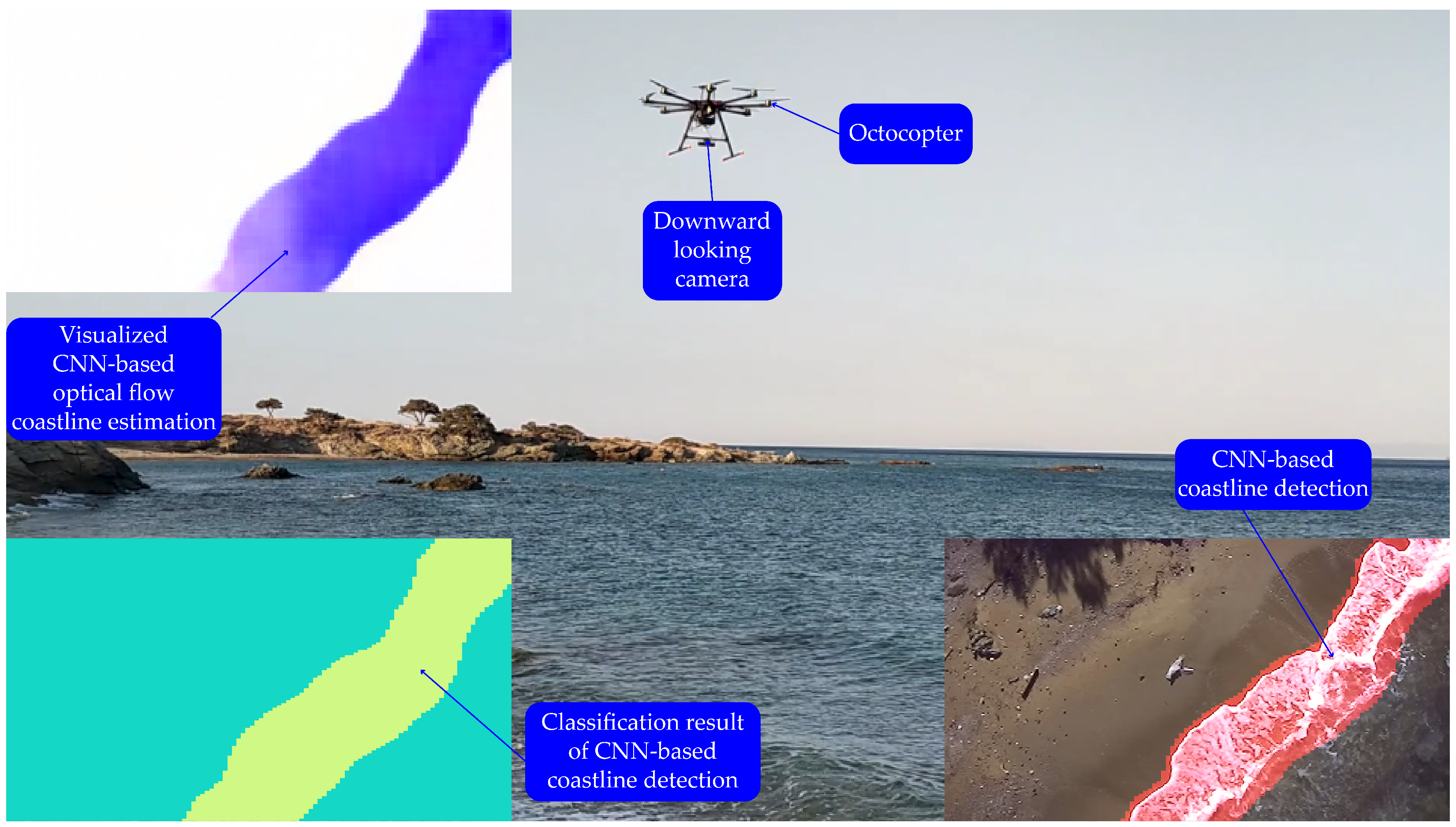
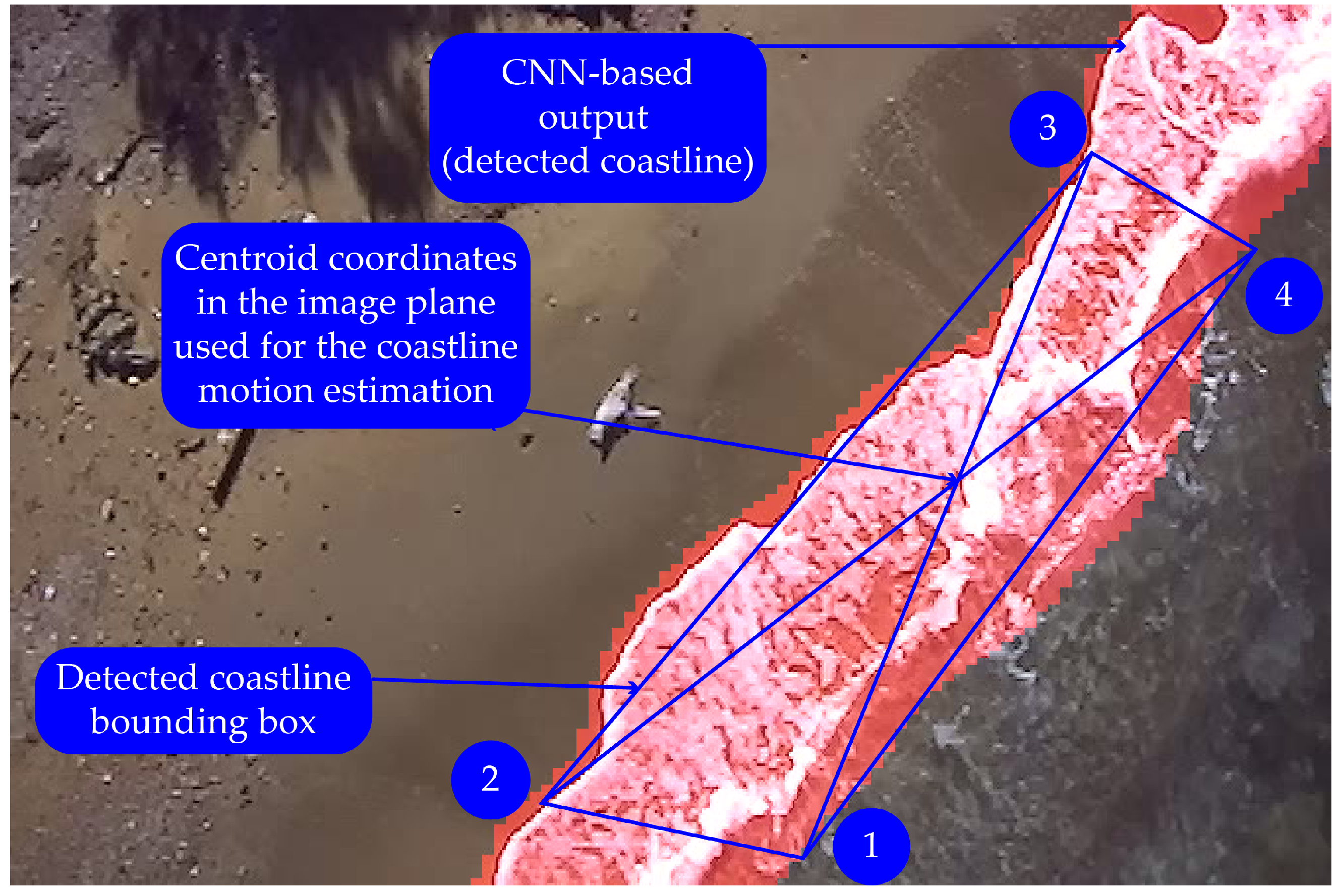
4.1. CNN-Based Coastline Detection

A pre-trained CNN for image segmentation is employed to achieve reliable coastline detection [45]. The CNN divides an image’s total pixels into relevant object classes. In order to accomplish specific tasks, the sequence of CNN layers undergoes end-to-end learning. The data is initially fed into the convolutional layer, including a learnable filter set. The result is normalized and sent to the pooling layer, which takes tiny data sets from the convolutional layer and samples the output of the chosen package’s result. The fully connected layers take up the high-level reasoning after a series of convolutional and pooling layers. Finally, backpropagation is used to learn CNN weights. The Keras image segmentation framework, specifically the pre-trained CNN model mobilenet_segnet, is used for image segmentation of the digital image recognizing the shoreline (Base Model: MobileNet and Segmentation Model: Segnet, an encoder network comprising 13 convolutional layers designed for object classification).

A data collection containing frames from the camera installed on the octocopter was utilized for training the selected CNN (Section 5.1). Training (7200 frames) and a validation (800 frames) data sets were created from the frames data set. The frames have a resolution of $672\times 376$ pixels. The following stages were included in the pre-processing procedure:

• Polygons are used to indicate the coastline through the labeling procedure.
• Masks are generated (binary images according to the annotated features from the labeling procedure).
• The frames were resized from $672\times 376$ pixels to $224\times 224$ pixels.
• Two-class classification (Class 0: Sea and Ground as black background on the mask and Class 1: Coastline).
• The training and validation sets were enhanced using a variety of augmentation methods.

Following the pre-processing, the CNN was trained on a computer with full GPU utilization until the CNN converged on the necessary accuracy after 10 epochs. On a raw image, the results of the trained CNN are shown in Figure 6. The trained CNN’s performance was validated by real-time prediction while flying above distinct coastlines.

The Region of Interest (ROI) can then be generated as a bounding box using standard image processing techniques [46] after a trained network offers online accurate shoreline detections. Calculating a bounding box serves two purposes: (i) specific feature matching across consecutive frames; (ii) minimization of PVS control features. The bounding box of the discovered coastline is depicted in Figure 6, with numbered corners $\mathbf{s}=\left[u_1,v_1,\cdots u_4,v_4\right]$. In order to formulate the feature error, these corners will be used in the PVS controller. In terms of individual feature velocity, this research concentrated on estimating the centroid velocity of the bounding box. It is predicted that its motion will adequately capture the individual velocity of its corners and the coastline portion enclosed therein. We separate the centroid measurements, which are the following:

$$\begin{array}{c}\hfill z_{u_{bc}}=\frac{1}{4}\sum _{n=1}^4{u}_i,z_{v_{bc}}=\frac{1}{4}\sum _{n=1}^4{v}_i\end{array}$$

(10)

and the individual velocity of the centroid, after removing the induced motion from the vehicle:

$$\begin{array}{c}\hfill {\mathbf{z}}_{\mathbf{v}}=\left[\begin{array}{c}{z}_{{\dot{u}}_{bc}}\\ z_{{\dot{v}}_{bc}}\end{array}\right]=\left[\begin{array}{c}\frac{z_{u_{bc}}\left(t\right)-z_{u_{bc}}(t-\mathsf{\Delta }t)}{\mathsf{\Delta }t}\\ \frac{z_{v_{bc}}\left(t\right)-z_{v_{bc}}(t-\mathsf{\Delta }t)}{\mathsf{\Delta }t}\end{array}\right]-\widehat{{\mathbf{L}}_{\mathbf{bc}}}\widehat{{\mathbf{v}}_{\mathbf{c}}}\end{array}$$

(11)

where, $\widehat{{\mathbf{L}}_{\mathbf{bc}}}\in {\Re }^{2\times 6}$ and $\widehat{{\mathbf{v}}_{\mathbf{c}}}$ are approximations of the interaction matrix for the centroid and the octorotor’s velocity, respectively, and $\mathsf{\Delta }t$ is the time interval between two consecutive centroid position detection measurements. Equation (11) is the initial method of estimating, and without the use of a corresponding algorithm, the $\widehat{\frac{\partial \mathbf{e}}{\partial \mathbf{t}}}$ for all cases of visual servoing tracking tasks.

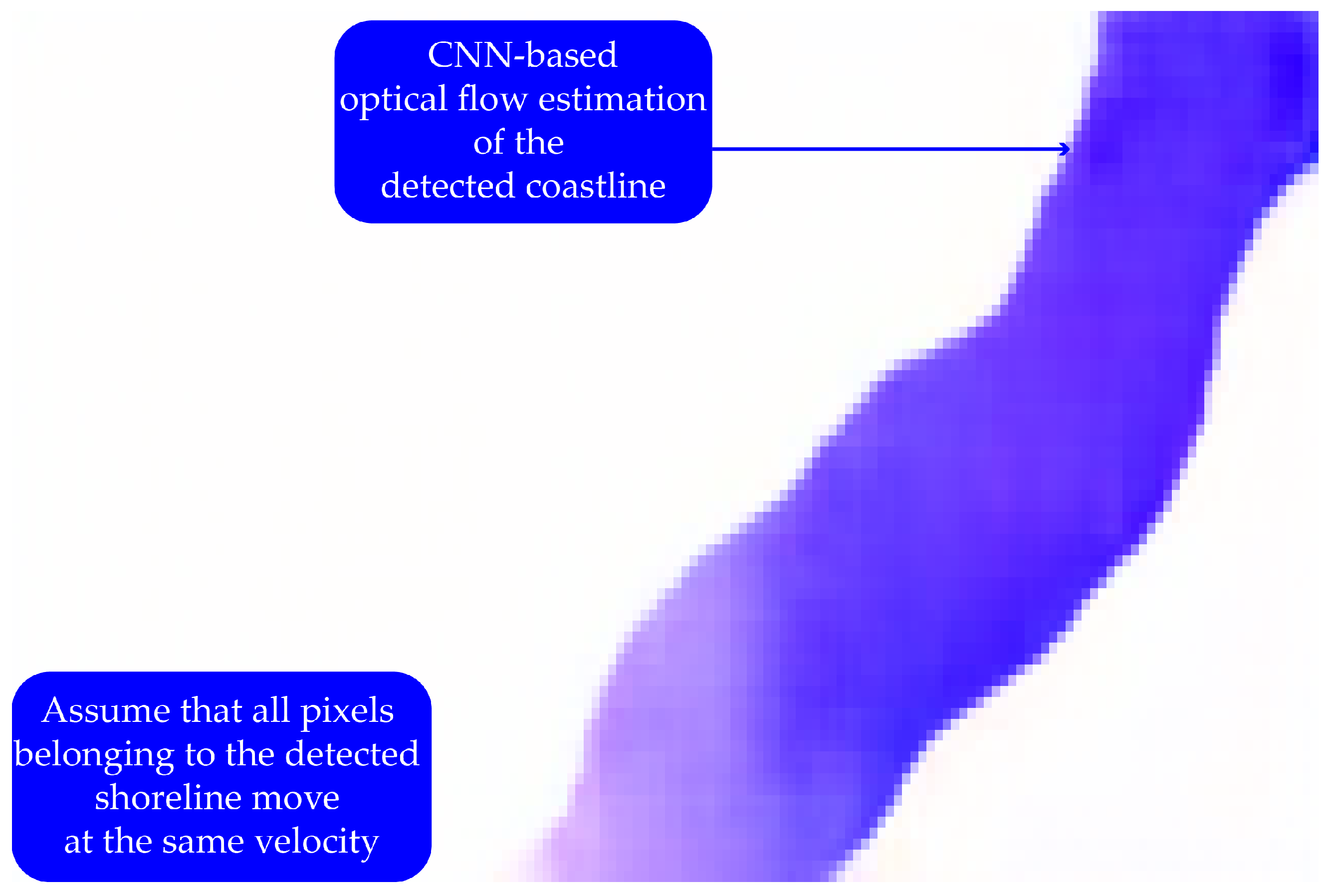
4.2. CNN-Based Coastline Optical Flow Estimation

As presented in Section 1.1, FlowNet 2 is as accurate as other state-of-the-art approaches while being faster. Utilizing FlowNet 2 and introducing as input pairs of images from the output of CNN presented in Section 4.1 results in the optical flow field estimation on the image plane.

Figure 7 depicts the visualized output of the CNN-based optical flow estimation. The optical flow estimate is based on the segmented image resulting in the part that does not belong to the shoreline (Class 0 according to Section 4.1) being colored white. In contrast, the shoreline is colored according to the value of the optical flow (purple in the case of Figure 7).

Assuming that all the pixels belonging to the detected coastline move evenly, we can use the optical flow field average for the target state estimation. The average flow rate obtained from FlowNet 2 by subtracting vehicle odometry provides a coarse data-driven approximation of the coastline wave motion (alternatively, is the data-driven estimate of (11)).

Domain knowledge, such as structured state-space models, is not included in a principled way by DNNs (e.g., FlowNet 2). As a result, even for simple sequences, these data-driven approaches necessitate a high number of trainable parameters and big data sets and thus lack the interpretability of model-based methods. Due to these constraints, the use of highly parametrized DNNs for real-time state estimation in applications integrated into hardware-constrained mobile devices like drones and vehicular systems is limited.

Therefore, the aforementioned data-driven approach will not be used as a standalone tool for the velocity estimation of the coastline. Instead, it will be incorporated as input to a neural network-aided EKF, as it will be presented in detail in Section 4.4. They are combined with an approximate wave motion model as described in Section 4.3 to provide a complete state estimation vector (i.e., position and velocity) of the coastline. This feedback will be further integrated into the proposed PVS control strategy to achieve autonomous coastline surveillance with the octocopter vehicle.

4.3. EKF-Based Coastline Motion Estimation

The formulation of an EKF online estimation of shoreline motion, directly in the image plane, using a wave motion model and measurements from the CNN detection and optical flow estimation frameworks is explained in this section. The wind, which creates waves on the water surface, causes the coastline to move individually. According to the mesh that depicts the ocean surface, it can be thought of as particles that follow a trajectory specified by the following equations, according to the Gerstner wave modeling approach [47]:

$$\begin{array}{cc}\hfill X_w& =X_{w_o}+\sum _{n=0}^N{a}_n{k}_{w_{x_n}}sin\left({\omega }_{n}t-{\mathbf{k}}_{{\mathbf{w}}_{\mathbf{n}}}·{\mathbf{P}}_{{\mathbf{w}}_{\mathbf{o}}}\right)\hfill \end{array}$$

(12)

$$\begin{array}{cc}\hfill Y_w& =Y_{w_o}+\sum _{n=0}^N{a}_n{k}_{w_{y_n}}sin\left({\omega }_{n}t-{\mathbf{k}}_{{\mathbf{w}}_{\mathbf{n}}}·{\mathbf{P}}_{{\mathbf{w}}_{\mathbf{o}}}\right)\hfill \end{array}$$

(13)

$$\begin{array}{cc}\hfill Z_w& =Z_{w_o}+\sum _{n=0}^N{a}_{n}sin\left({\omega }_{n}t-{\mathbf{k}}_{{\mathbf{w}}_{\mathbf{n}}}·{\mathbf{P}}_{{\mathbf{w}}_{\mathbf{o}}}\right)\hfill \end{array}$$

(14)

where ${\mathbf{P}}_{{\mathbf{w}}_{\mathbf{o}}}={\left[X_{w_o},Y_{w_o}\right]}^T$ describes the particle’s resting position on the suface, while $Z_{w_o}$ is the altitude’s last resting place, $a_n$ the amplitude, $\frac{{\omega }_n}{2\pi }$ the frequency and ${\mathbf{k}}_{{\mathbf{w}}_{\mathbf{n}}}={\left[k_{w_{x_n}},k_{w_{y_n}}\right]}^T$ the direction unit vector for the surface wave components. Only the tracking of surface motion was important in the surveillance application studied in this work, not the altitude of the coastline. After that, the following practical considerations are made:

• The bounding box centroid, which is part of the shoreline, is the projection of a water particle ${\mathbf{P}}_{\mathbf{bc}}={\left[X_{bc},Y_{bc}\right]}^T$, which has a rest location ${\mathbf{P}}_{{\mathbf{bc}}_{\mathbf{o}}}={\left[X_{b{c}_o},Y_{b{c}_o}\right]}^T$, and so follows the Gerstner wave model.
• We consider that there is just one dominant frequency ${\omega }_{bc}$ that impacts the wave’s amplitude $a_{bc}$, while the other frequencies have a tiny contribution and may thus be ignored.
• The waves’ direction is constant throughout time, therefore ${\mathbf{k}}_{\mathbf{w}}={\mathbf{k}}_{\mathbf{bc}}=const$. The constant phase terms ${\varphi }_{w_x}$, ${\varphi }_{w_y}$ appear in the sinusoidal terms of the surface position components $X_w$, $Y_w$, respectively.

As a result, using the Equation set (12) and (13) to explain the centroid’s surface motion while taking into account the previous considerations yields:

$$\begin{array}{c}\hfill X_{bc}=X_{b{c}_o}+a_{bc}{k}_{b{c}_x}sin\left({\omega }_{bc}t-{\varphi }_{bc}\right)\end{array}$$

(15)

$$\begin{array}{c}\hfill Y_{bc}=Y_{b{c}_o}+a_{bc}{k}_{b{c}_y}sin\left({\omega }_{bc}t-{\varphi }_{bc}\right)\end{array}$$

(16)

where ${\varphi }_{bc}={\mathbf{k}}_{\mathbf{bc}}·{\mathbf{P}}_{{\mathbf{bc}}_{\mathbf{o}}}$, with ${\mathbf{k}}_{\mathbf{bc}}={\left[k_{b{c}_x},k_{b{c}_y}\right]}^T$. Using the camera model Equation (3) and the appropriate algebraic manipulations, the projection of the centroid in the image plane is represented as follows:

$$\begin{array}{c}\hfill u_{bc}=u_{b{c}_o}+A_{b{c}_u}sin\left({\omega }_{bc}t-{\varphi }_{bc}\right)\end{array}$$

(17)

$$\begin{array}{c}\hfill v_{bc}=v_{b{c}_o}+A_{b{c}_v}sin\left({\omega }_{bc}t-{\varphi }_{bc}\right)\end{array}$$

(18)

where: $u_{b{c}_o}=c_u+\frac{{\alpha }_x{X}_{b{c}_o}}{Z_{bc}}$, $v_{b{c}_o}=c_v+\frac{{\alpha }_y{Y}_{b{c}_o}}{Z_{bc}}$, $A_{b{c}_u}=\frac{{\alpha }_x{a}_{bc}}{Z_{bc}}{k}_{b{c}_x}$, $A_{b{c}_v}=\frac{{\alpha }_y{a}_{bc}}{Z_{bc}}{k}_{b{c}_y}$. The purpose is to design an EKF in order to achieve an estimation of the centroid velocity. Next, we define the system and measurement models for the proposed estimator.

4.3.1. System Model

Taking the Equation set (17) and (18) and calculating the two times derivatives with respect to time, the following harmonic oscillation models with constant dump terms, which describe the coastline motion are obtained:

$$\begin{array}{c}\hfill {\ddot{u}}_{bc}=-{\omega }_{bc}^2{u}_{bc}+{\omega }_{bc}^2{u}_{b{c}_o}\end{array}$$

(19)

$$\begin{array}{c}\hfill {\ddot{v}}_{bc}=-{\omega }_{bc}^2{v}_{bc}+{\omega }_{bc}^2{v}_{b{c}_o}\end{array}$$

(20)

Considering the state vector $\mathbf{m}={[u_{bc},{\dot{u}}_{bc},v_{bc},{\dot{v}}_{bc},{\omega }_{bc},u_{b{c}_o},v_{b{c}_o}]}^T$, and the terms ${\omega }_{bc}$,$u_{b{c}_o}$, $v_{b{c}_o}$ to be constant over time, the non-linear system model is formulated as follows:

$$\dot{\mathbf{m}}=\mathbf{f}\left(\mathbf{m}\right)\mathbf{m}$$

(21)

More specifically, by invoking (19) and (20) and considering ${\omega }_{bc},u_{b{c}_o},v_{b{c}_o}$ to be constant over time, we formulate the following state-space form of the system, which is clearly non-linear:

$$\left[\begin{array}{c}{\dot{u}}_{bc}\\ {\ddot{u}}_{bc}\\ {\dot{v}}_{bc}\\ {\ddot{v}}_{bc}\\ {\dot{\omega }}_{bc}\\ {\dot{u}}_{b{c}_o}\\ {\dot{v}}_{b{c}_o}\end{array}\right]=\left[\begin{array}{ccccccc}0& 1& 0& 0& 0& 0& 0\\ -{\omega }_{bc}^2& 0& 0& 0& 0& {\omega }_{bc}^2& 0\\ 0& 0& 0& 1& 0& 0& 0\\ 0& 0& -{\omega }_{bc}^2& 0& 0& 0& {\omega }_{bc}^2\\ 0& 0& 0& 0& 0& 0& 0\\ 0& 0& 0& 0& 0& 0& 0\\ 0& 0& 0& 0& 0& 0& 0\end{array}\right]\left[\begin{array}{c}{u}_{bc}\\ {\dot{u}}_{bc}\\ v_{bc}\\ {\dot{v}}_{bc}\\ {\omega }_{bc}\\ u_{b{c}_o}\\ v_{b{c}_o}\end{array}\right]$$

(22)

The system dynamics matrix can be approximated by the Jacobian matrix $\mathbf{F}=\frac{\partial \mathbf{f}\left(\mathbf{m}\right)}{\partial \mathbf{m}}$

$$\mathbf{F}=\frac{\partial f\left(\mathbf{m}\right)}{\partial \mathbf{m}}=\left[\begin{array}{ccccccc}0& 1& 0& 0& 0& 0& 0\\ -\widehat{{\omega }_{bc}^2}& 0& 0& 0-2\widehat{{\omega }_{bv}}\widehat{u_{bc}}+2\widehat{{\omega }_{bv}}\widehat{u_{b{c}_o}}& \widehat{{\omega }_{bc}^2}\\ 0& 0& 0& 1& 0& 0& 0\\ 0& 0& -\widehat{{\omega }_{bc}^2}& -2\widehat{{\omega }_{bv}}\widehat{v_{bc}}+2\widehat{{\omega }_{bv}}\widehat{v_{b{c}_o}}& 0& \widehat{{\omega }_{bc}^2}\\ 0& 0& 0& 0& 0& 0& 0\\ 0& 0& 0& 0& 0& 0& 0\\ 0& 0& 0& 0& 0& 0& 0\end{array}\right]$$

(23)

the terms of $\mathbf{F}$ have been evaluated at the current state estimates. Assuming that the elements of $\mathbf{F}$ are approximately constant between the sampling interval $T_s$, then a two-term—Taylor series to approximate the fundamental matrix, in discrete form ${\mathrm{\Phi }}_k\approx \mathbf{I}+\mathbf{F}{T}_s$ can be employed. Hence, the discrete system model is approximated as follows:

$${\mathbf{m}}_{\mathbf{k}}={\mathrm{\Phi }}_k{\mathbf{m}}_{\mathbf{k}-\mathbf{1}}+{\mathbf{w}}_{\mathbf{k}}$$

(24)

where ${\mathbf{w}}_{\mathbf{k}}$ is the process noise, which is assumed to be drawn from a zero mean multivariate normal distribution, with covariance, ${\mathbf{Q}}_{\mathbf{k}}:{\mathbf{w}}_k\sim \mathcal{N}\left(0,{\mathbf{Q}}_k\right)$.

4.3.2. Measurement Model

The measurement vector is defined as:

$${\mathbf{z}}_{\mathbf{bc}}={\left[z_{u_{bc}},z_{v_{bc}},z_{{\dot{u}}_{bc}},z_{{\dot{v}}_{bc}}\right]}^T$$

(25)

where $z_{u_{bc}},z_{v_{bc}}$ are the centroid coordinates in image space as determined by the CNN, and $z_{{\dot{u}}_{bc}},z_{{\dot{v}}_{bc}}$ are the respective velocities after removing the influence of camera motion, as stated in Section 4.1. These measures are related to the EKF’s estimated states in the following way:

$${\mathbf{z}}_{{\mathbf{bc}}_{\mathbf{k}}}={\mathbf{H}}_{\mathbf{k}}\widehat{{\mathbf{m}}_{\mathbf{k}}}+{\upsilon }_k$$

(26)

where ${\mathbf{H}}_{\mathbf{k}}$ is a constant matrix and ${\upsilon }_k$ is the measurement noise, which is assumed to be drawn from a zero mean multivariate normal distribution, with covariance, ${\mathbf{R}}_{\mathbf{k}}:{\upsilon }_k\sim \mathcal{N}\left(0,{\mathbf{R}}_k\right)$.

4.3.3. State Update

The next step is the calculation of the Kalman gain ${\mathbf{K}}_{\mathbf{k}}$, which is obtained from the following recursive set of discrete equations:

$$\begin{array}{c}\hfill {\mathbf{M}}_{\mathbf{k}}={\mathrm{\Phi }}_k{\mathbf{P}}_{\mathbf{k}-\mathbf{1}}{{\mathrm{\Phi }}_k}^T+{\mathbf{Q}}_{\mathbf{k}}\end{array}$$

(27)

$$\begin{array}{c}\hfill {\mathbf{K}}_{\mathbf{k}}={\mathbf{M}}_{\mathbf{k}}{\mathbf{H}}_{\mathbf{k}}^T{\left({\mathbf{H}}_{\mathbf{k}}{\mathbf{M}}_{\mathbf{k}}{\mathbf{H}}_{\mathbf{k}}^T+{\mathbf{R}}_{\mathbf{k}}\right)}^{-1}\end{array}$$

(28)

$$\begin{array}{c}\hfill {\mathbf{P}}_{\mathbf{k}}=\left(\mathbf{I}-{\mathbf{K}}_{\mathbf{k}}{\mathbf{H}}_{\mathbf{k}}\right){\mathbf{M}}_{\mathbf{k}}\end{array}$$

(29)

where ${\mathbf{P}}_{\mathbf{k}}$ is the state estimate covariance matrix. The following equation is used to determine the state update:

$${\widehat{\mathbf{m}}}_{\mathbf{k}}={\mathrm{\Phi }}_k{\widehat{\mathbf{m}}}_{\mathbf{k}-\mathbf{1}}+{\mathbf{K}}_{\mathbf{k}}\left({\mathbf{z}}_{{\mathbf{bc}}_{\mathbf{k}}}-{\mathbf{H}}_{\mathbf{k}}{\mathrm{\Phi }}_k{\widehat{\mathbf{m}}}_{\mathbf{k}-\mathbf{1}}\right)$$

(30)

The vector ${\widehat{\mathbf{m}}}_{\mathbf{k}}$ comprises updated estimates of the target’s (bounding box) centroid’s position and velocity, as well as updates on the frequency and offsets caused by the waves’ sinusoidal motion of the shoreline. In the case of standalone model-based EKF utilization, in order to synthesize vector $\widehat{\frac{\partial \mathbf{s}}{\partial \mathbf{t}}}$ and the estimated error vector $\widehat{\frac{\partial \mathbf{e}}{\partial \mathbf{t}}}$, we use the estimates ${\widehat{\dot{u}}}_{bc}$ and ${\widehat{\dot{v}}}_{bc}$. The presented EKF formulation comprises the model-based part EKF estimator presented in the following Section 4.4 and finally the estimated error vector $\widehat{\frac{\partial \mathbf{e}}{\partial \mathbf{t}}}$ is utilized in the PVS tracking control strategy presented in Section 4.5.

Remark 2.

The proposed EKF-based estimation technique can be employed for the centroid and all the corners of the bounding box. In such a case, estimating the four corner positions and velocities can be incorporated into an image-based control scheme. However, this will increase complexity and computational cost without significant performance improvements.

4.4. Neural Network Aided Kalman Filtering for Coastline Motion Estimation

4.4.1. Preliminaries

The core module of the proposed framework (Figure 5) is the neural network-aided Kalman filtering for coastline motion estimation presented in this section. In this case, the specific module results in formulating and adapting the hybrid MB/DD online recursive filter called KalmanNet, which leverages data and partial domain knowledge to learn the Extended Kalman Filtering operation. The formulated KalmanNet is presented in Section 4.3 rather than using data to directly estimate the missing state-space model parameters, as stated in Section 1.1. KalmanNet initially concentrates on nonlinear, Gaussian, and continuous state-space models, which are represented as follows for each $t\in \mathbb{Z}$:

$$\begin{array}{c}\hfill {\mathbf{x}}_t=\mathbf{f}\left({\mathbf{x}}_{t-1}\right)+{\mathbf{w}}_t,{\mathbf{w}}_t\sim \mathcal{N}(0,\mathbf{Q}),{\mathbf{x}}_t\in {\mathbb{R}}^m\end{array}$$

(31)

$$\begin{array}{c}\hfill {\mathbf{y}}_t=\mathbf{h}\left({\mathbf{x}}_t\right)+{\mathbf{v}}_t,{\mathbf{v}}_t\sim \mathcal{N}(0,\mathbf{R}),{\mathbf{y}}_t\in {\mathbb{R}}^n\end{array}$$

(32)

where ${\mathbf{x}}_t$ is the system’s latent state vector at time t, which evolves from the previous state ${\mathbf{x}}_{t-1}$ via a non-linear state-evolution function $\mathbf{f}(·)$ and a white gaussian noise ${\mathbf{w}}_t$ with covariance matrix $\mathbf{Q}$. The vector of observations at time t is ${\mathbf{y}}_t$, which is created from the current latent state vector by a non-linear observation mapping $\mathbf{h}(·)$ corrupted by additional white gaussian noise ${\mathbf{v}}_t$ with covariance $\mathbf{R}$.

State-space models are investigated in the context of various tasks, all of which are distinct and may be loosely divided into two categories: observation approximation and hidden state recovery. The first category is concerned with estimating portions of the observed signal ${\mathbf{y}}_t$ and can include predicting future data based on previous observations, generating missing observations in a block via imputation, and denoising the observations. The recovery of a concealed state vector ${\mathbf{x}}_t$ falls under the second.

The filtering issue is crucial to real-time tracking. In this case, one must produce a quick online estimate of the state ${\mathbf{x}}_t$ based on each incoming observation ${\mathbf{y}}_t$. Our main focus is on cases in which the state-space model representing the underlying dynamics is only partially known. The state-evolution (transition) function $\mathbf{f}(·)$ and the state-observation (emission) function $\mathbf{h}(·)$ are two functions we know (or have an estimate of). This expertise is obtained from our understanding of the system dynamics, physical design, and sensor model for real-world applications. The noise statistics $\mathbf{Q}$ and $\mathbf{R}$ are unknown, in contrast to the traditional assumptions in KF. We assume, more specifically:

• There is no knowledge of the distribution of the noise signals ${\mathbf{w}}_t$ and ${\mathbf{v}}_t$.
• The functions $\mathbf{f}(·)$ and $\mathbf{h}(·)$ could be used to approximate the true underlying dynamics. Approximations of this type can be used to depict continuous-time dynamics in discrete time, acquire data with misaligned sensors, and other types of mismatches.

4.4.2. Hybrid MB/DD Real-Time Estimator Formulation

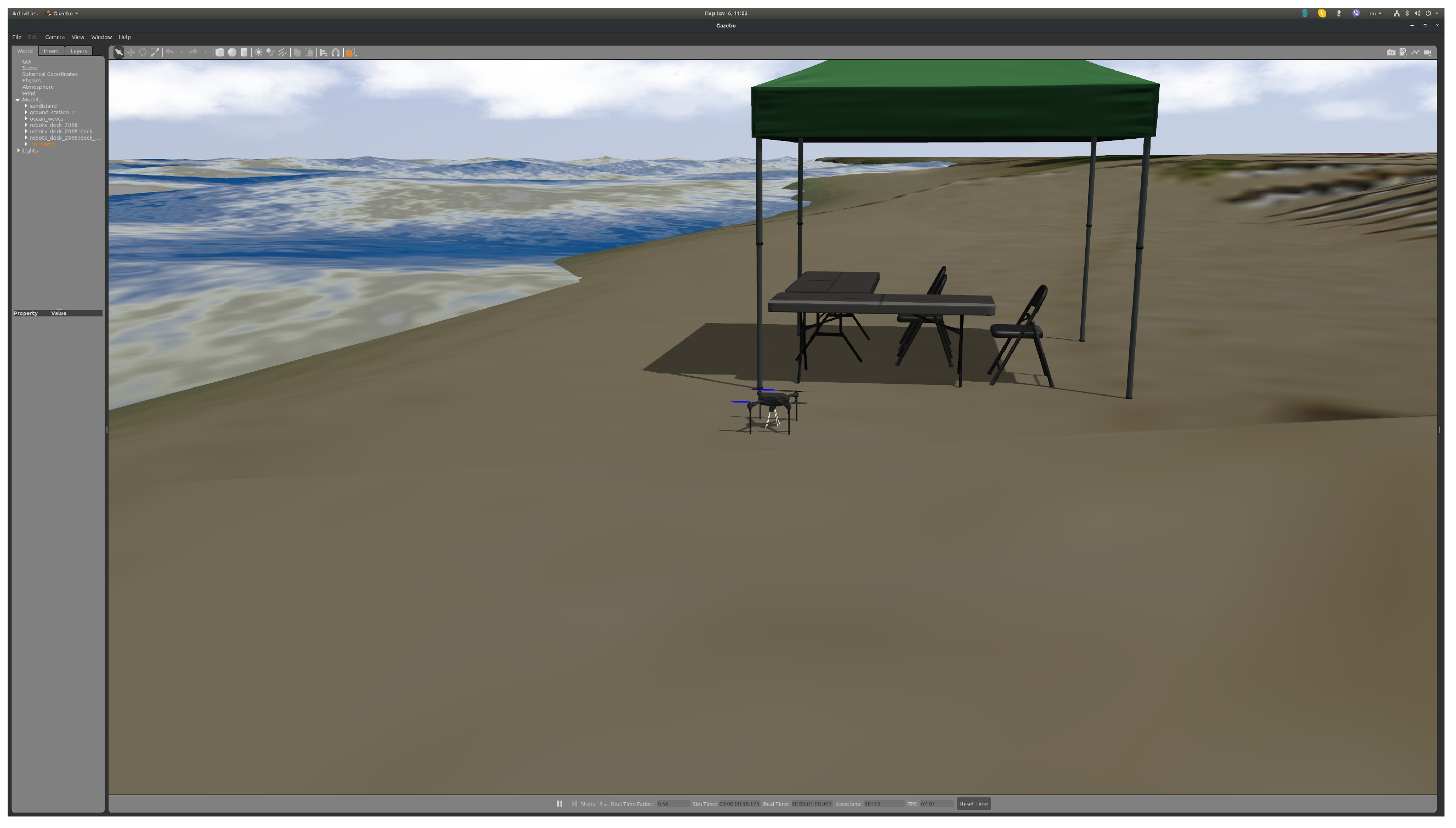
The utilization of KalmanNet in the case of coastline waves begins with defining the system that represents its motion. According to the analytical EKF formulation presented in Section 4.3, the shoreline dynamic wave motion system is defined through the harmonic oscillator (19) and (24). Furthermore, the measurement model is represented via (26) and (25).

We formulate KalmanNet by identifying the specific computations of the EKF that are based on unavailable knowledge. The corresponding functions $\mathbf{f}(·)$ and $\mathbf{h}(·)$ are known (Gerstner waves model assumption and measurement model, respectively); yet the corresponding covariance matrices $\mathbf{Q}$ and $\mathbf{R}$ are unavailable. These missing statistical moments are used in model-based Extended Kalman Filtering only for computing the Kalman Gain via the use of (28). Thus, the KalmanNet learns Kalman Gain from data and combines the learned Kalman Gain in the overall Extended Kalman Filter flow. In each time step t, similarly to the EKF, KalmanNet estimates ${\widehat{\mathbf{m}}}_{\mathbf{k}}$ in two steps; prediction and update.

Only the first-order statistical moments are predicted, as opposed to the model-based Extended Kalman Filter. Specifically, the previous posterior ${\widehat{\mathbf{m}}}_{\mathbf{k}-\mathbf{1}}$ is used to generate a prior estimate for the present state ${\widehat{\mathbf{m}}}_{\mathbf{k}|\mathbf{k}-\mathbf{1}}$. Then, using ${\widehat{\mathbf{m}}}_{\mathbf{k}|\mathbf{k}-\mathbf{1}}$, a previous estimate for the current measurement ${\mathbf{z}}_{b{c}_k}$ is computed. KalmanNet, unlike its model-based predecessors, does not rely on noise distribution information and does not keep a precise estimate of second-order statistical moments.

Similar to the model-based EKF and the Kalman Gain ${\mathbf{K}}_k$, KalmanNet uses the new measurement ${\mathbf{z}}_{{bc}_k}$ to compute the current state posterior ${\widehat{\mathbf{m}}}_k$ from the previously computed prior ${\widehat{\mathbf{m}}}_{k|k-1}$ in the update step. In contrast to the model-based EKF, the Kalman Gain is not explicitly computed; instead, it is learned from data using an RNN. RNN’s built-in memory allows them to track second-order statistical moments without knowing the underlying noise statistics.

4.4.3. Simulator

As mentioned above, the data-driven part of the hybrid MB/DD real-time estimator requires RNN training that learns Kalman Gain calculation with labeled data. A labeled dataset is initially created to achieve the training. The process of collecting this data and creating the set (shown below) took place in a synthetic environment of a realistic coastline and flight simulation of a UAV. Hence, this section presents the synthetic realistic environment development and data collection process, aiming at the required RNN training. The overall development and utilization of simulation environments for autonomous flight applications are due to the following reasons:

• safety reasons → increased risk of vehicle crash during the early testing of prototype autonomous flight algorithms
• logistics problems while rapid prototyping → inability to conduct experiments frequently (e.g., every day) along the coast

In order to expedite the development process, a synthetic but realistic coastline simulation environment (Figure 8) was built using the Robot Operating System (ROS) [48] and Gazebo [49] frameworks, featuring also MAVROS [50] communication protocol as SITL. The synthetic environment is based on [51] featuring a coastline with configurable parameters for the waves (i.e., peak period, gain, direction, etc.), the wind velocity, and the fog and ambient visual conditions. A 3DR Iris quadrotor [52] is deployed inside the simulation environment equipped with the appropriate sensor suite:

• Navigation sensors (GPS, IMU, altimeter, etc.)
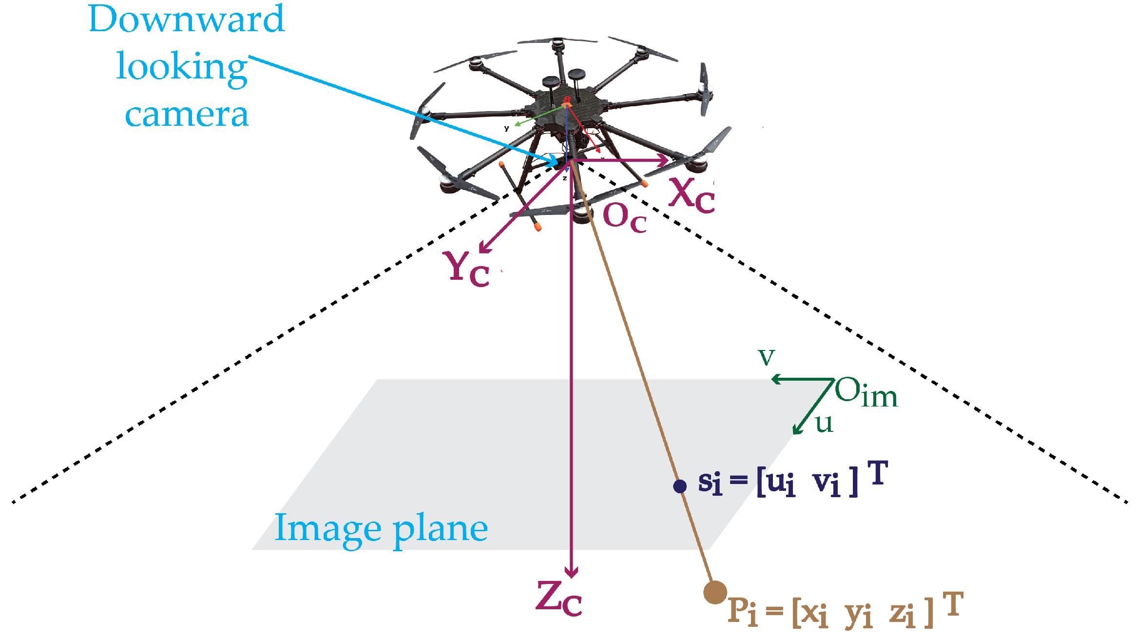
• Downward-looking stereo camera system (ZED 2), providing frame-based image data

In this flight simulation environment, the vehicle can be remote-controlled by the user, while at the same time, the following data is collected online:

• Position of the pixels belonging to the coastline, which results from the outcome of the CNN-based coastline detection module.
• Approximation of the $\widehat{\frac{\partial \mathbf{e}}{\partial \mathbf{t}}}$ vector, which results from the outcome of the CNN-based optical flow of the pixels belonging to the detected coastline after subtracting the vehicle velocity.

Collecting the data above leads to creating the dataset for the RNN training of the Kalman Gain calculation, which will be presented in the following Section 4.4.4.

4.4.4. Training & Deployment

The Kalman Gain is computed by the model-based EKF and its variants using knowledge of the underlying data. To execute such computations in a learning manner, one must supply input to a neural network that captures the knowledge required to evaluate Kalman Gain. Because ${\mathbf{K}}_k$ is dependent on the statistics of the observations and the state process, the RNN should be fed statistical information from the measurement ${\mathbf{z}}_{b{c}_k}$ and the state estimate ${\widehat{\mathbf{m}}}_{k-1}$ at each time step t. As a result, the following features connected to the state-space model’s unknown statistical relationship can be employed as RNN input features:

• Feature 1: The measurement difference $\mathsf{\Delta }{\tilde{\mathbf{z}}}_{b{c}_k}={\mathbf{z}}_{b{c}_k}-{\mathbf{z}}_{b{c}_{k-1}}$.
• Feature 2: The innovation difference $\mathsf{\Delta }{\mathbf{z}}_{b{c}_k}={\mathbf{z}}_{b{c}_k}-{\widehat{\mathbf{z}}}_{b{c}_{k|k-1}}$.
• Feature 3: The forward evolution difference $\mathsf{\Delta }{\tilde{\mathbf{m}}}_k={\widehat{\mathbf{m}}}_{k|k}-{\widehat{\mathbf{m}}}_{k-1|k-1}$. This value reflects the difference between two successive posterior state estimates, where the accessible feature for time instance t is $\mathsf{\Delta }{\tilde{\mathbf{m}}}_{k-1}$.
• Feature 4: The forward update difference $\mathsf{\Delta }{\widehat{\mathbf{m}}}_k={\widehat{\mathbf{m}}}_{k|k}-{\widehat{\mathbf{m}}}_{k|k-1}$, i.e., the difference between the posterior state estimate and the prior state estimate, where $\mathsf{\Delta }{\widehat{\mathbf{m}}}_{k-1}$ is used for the time step t.

Features 1 and 3 contain information on the state evolution process, whereas features 2 and 4 contain information about the uncertainty of our state estimate. Because the difference operation removes predictable components, the time series of differences is mainly influenced by the noise statistics we want to learn.

The ${\mathbf{K}}_k$ is determined by keeping track of second-order statistical moments. Because the Kalman Gain computation is recursive, an internal memory element such as an RNN should be utilized to track it. KalmanNet is trained in a supervised manner utilizing the generated dataset. Even though we use a neural network to compute the Kalman Gain rather than simply producing the estimate ${\widehat{\mathbf{m}}}_{k|k}$, we train KalmanNet from start to finish. The state estimate ${\widehat{\mathbf{m}}}_k$, which is not the output of the internal RNN, is used to compute the loss function. We employ the backpropagation through time (BPTT) approach to train KalmanNet since it is a recursive design with both an external recurrence and an internal RNN. A forward and backward gradient estimate run through the network is computed when KalmanNet is unfolded across time using shared network parameters.

KalmanNet is a data-driven/model-based hybrid that, in our application, is formulated to combine deep learning with the traditional EKF-based coastal motion estimating approach. It benefits from the individual capabilities of both data-driven and model-based techniques by identifying the specific noise-model-dependent calculations of the EKF and replacing them with a dedicated RNN integrated into the EKF flow. KalmanNet and its model-based equivalent have numerous key distinctions due to the addition of specialized deep learning modules to the EKF. Unlike the model-based EKF, it does not try to linearize the SS model or impose a statistical model on the noisy signals. Moreover, KalmanNet filters in a nonlinear manner because its KG matrix is dependent on the input ${\mathbf{z}}_{b{c}_k}$ and it is more resilient to model mismatch than the traditional model-based Kalman.

For the case of the shoreline, we deploy the so presented KalmanNet through the combination of the CNN-based optical flow estimation (Section 4.2), the EKF formulation (Section 4.3), and the integration and adaptation of KalmanNet based on the specific data. Keeping in mind the hypothesis of Gerstner waves (coarse estimation of the state-space model), we generated the optimal estimation of the motion of the coastline.

From data provided by CNN-based shoreline detection and the related optical flow estimation, we generated a dataset by configuring Features 1, 2, 3, and 4 as explained. The dataset is made up of a training set with a length of 100-time steps and a test set with a length of 1000 time steps. The model was trained on a PC with the GPU fully utilized up to the required MMSE convergence after 200 seasons.

The state-evolution parameters employed by the filters differ somewhat from the genuine model in the presence of incomplete model information (Gerstner waves model of motion), resulting in a significant reduction in the model-based EKF due to the model mismatch. KalmanNet solves such mismatches in all studies, and its performance is comparable to that attained when complete information is available for such settings. In the presence of solid nonlinearities (e.g., Gerstner wave motion model) and model uncertainties due to erroneous approximation of the underlying dynamics. The model-based versions of the EKF fail, and KalmanNet learns to approach the MMSE while keeping the EKF’s real-time operation and low complexity.

The outcome of this procedure is integrated into the proposed PVS control strategy through the estimated error vector $\widehat{\frac{\partial \mathbf{e}}{\partial \mathbf{t}}}$, which will be presented in the following Section 4.5.

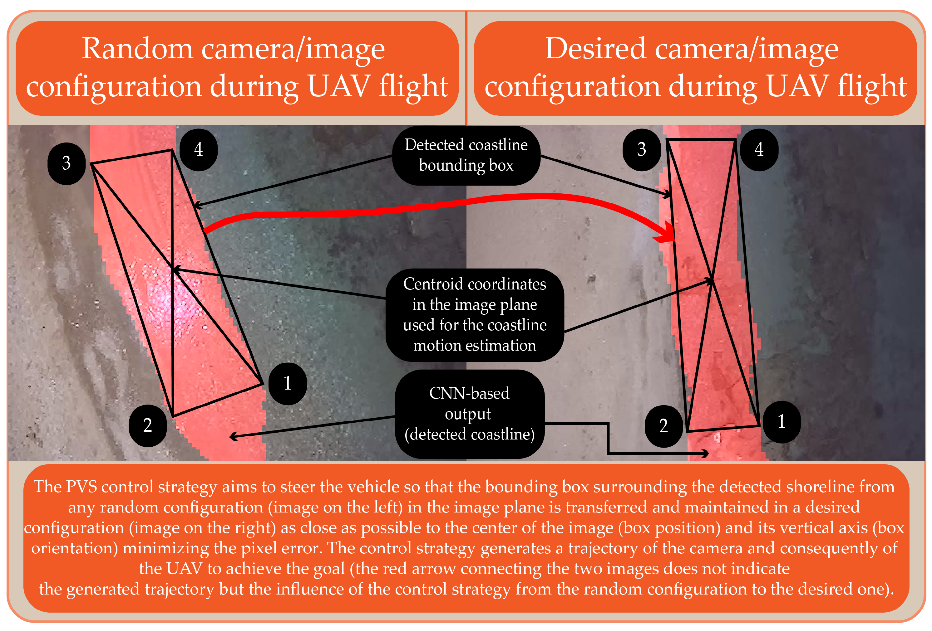
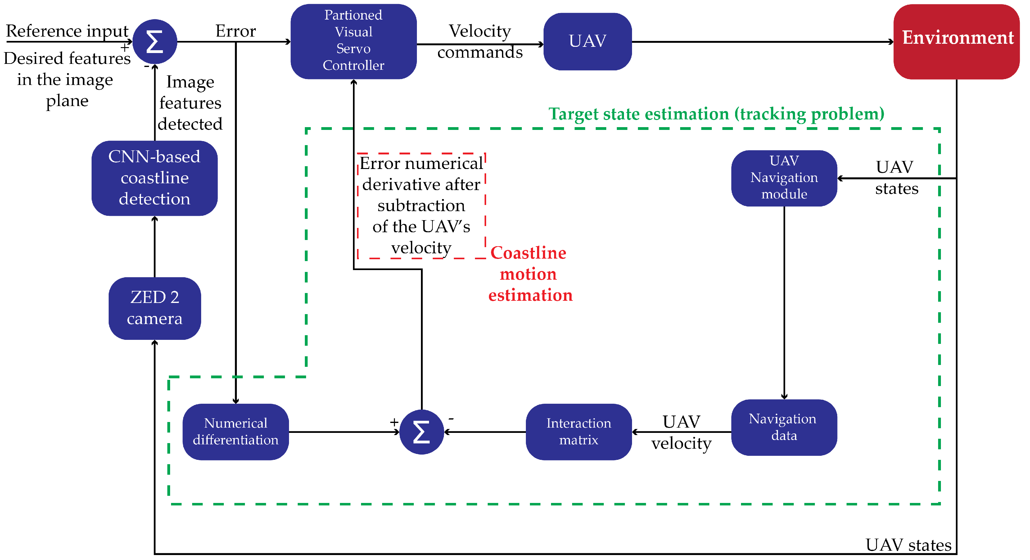
4.5. PVS Control Strategy

4.5.1. Control Development

The development of a PVS scheme for octocopter control is examined in this section. The controller must fulfill the following requirements:

• Successful tracking of a dynamic coastline.
• Handling of the motion caused from the coastline waves.
• Maintenance of the coastline as close as possible to the center of the camera’s FoV.

In accordance with the above objectives to be achieved, a PVS control method is developed aiming at the simultaneous stabilization and monitoring of the detected shoreline in the field of view, while the vehicle flies along the entire of a beach. Let the error be defined as $\mathbf{e}=\mathbf{s}-{\mathbf{s}}_{\mathbf{d}}$, where $\mathbf{s}={\left[u_1,v_1,\dots u_4,v_4\right]}^T$ the corners of the coastline bounding box and:

$${\mathbf{s}}_{\mathbf{d}}\left(\mathbf{t}\right)={\left[u_{d_1},v_{d_1}+{\upsilon }_{f}t,u_{d_2},v_{d_2}+{\upsilon }_{f}t,u_{d_3},v_{d_3}+{\upsilon }_{f}t,u_{d_4},v_{d_4}+{\upsilon }_{f}t\right]}^T$$

(33)

where ${\upsilon }_f$ is a tuning parameter, and t is the time in this simple planning profile. The octorotor’s additional velocity, expressed in the image plane, is controlled by the parameter ${\upsilon }_f$ in order to move forward along the shoreline.

The dynamics of the error in the image plane are presented via [8]:

$$\dot{\mathbf{e}}=\dot{\mathbf{s}}-{\dot{\mathbf{s}}}_{\mathbf{d}}\stackrel{}{\Rightarrow }\dot{\mathbf{e}}={\mathbf{L}}_{xy}{\mathbf{v}}_{xy}+{\mathbf{L}}_z{\mathbf{v}}_z+\frac{\partial \mathbf{e}}{\partial \mathbf{t}}-{\dot{\mathbf{s}}}_{\mathbf{d}}$$

(34)

The combination of (7) and the exponential error decrease $\dot{\mathbf{e}}=-k\mathbf{e}$ results to control law:

$${\mathbf{v}}_{xy}=-\widehat{{\mathbf{L}}_{xy}^{+}}\left(k\mathbf{e}-{\dot{\mathbf{s}}}_d+\widehat{\frac{\partial \mathbf{e}}{\partial \mathbf{t}}}+{\mathbf{L}}_z{\mathbf{v}}_z\right)$$

(35)

where

$${\mathbf{v}}_z=\left[v_z={\lambda }_{v_z}ln\left(\frac{{\sigma }^{*}}{\sigma }\right),{\omega }_z={\lambda }_{{\omega }_z}({\alpha }^{*}-\alpha )\right]$$

(36)

in which $\alpha$, with $0\le \alpha <2\pi$ is the angle between the horizontal axis of the image plane and the directed line segment joining two feature points, and ${\alpha }^{*}$ is the desired value of the angle, $\sigma$ the area of the bounding box defined by the coastline detected features and ${\sigma }^{*}$ its desired value.

The result of the employed PVS strategy is visualized in Figure 9. As it is shown, the calculations of planar and rotational velocities by (35) and (36), cause the execution of the image trajectory (depicted in Figure 9 with a red arrow) from a random (left side of Figure 9) to the desired configuration (right side of Figure 9) of the bounding box surrounding the detected coastline.

4.5.2. Stability Analysis

This section presents the proof of the stability analysis of the aforementioned PVS control scheme in (35) and (36). We start with the following theorem:

Theorem 1.

The dynamics of the error of the features on the image plane, i.e.,:

$$\dot{\mathbf{e}}={\mathbf{L}}_{xy}{\mathbf{v}}_{xy}+{\mathbf{L}}_z{\mathbf{v}}_z+\frac{\partial \mathbf{e}}{\partial \mathbf{t}}-{\dot{\mathbf{s}}}_{\mathbf{d}},$$

(37)

under the control laws (35) and (36) are asymptotically stable around zero.

Proof. 

As per the PVS scheme, the dynamics and control are split into two parts, namely relating to the planar and rotational motions around the $xy$ plane and the z axis of the camera frame, respectively. Therefore, we will reflect this core idea in the following stability analysis. First of all we treat the $xy$ dynamics. Considering the function $L_e={\parallel e\parallel }^2$, it is positive definite, for ${\mathbf{L}}_{xy}{\mathbf{v}}_{xy}\ne \mathbf{0}$, except for $\mathbf{e}=\mathbf{0}$, while its derivative, under the control law (35) can also be shown to be negative semi-definite at the same set: $\mathcal{E}=\{\mathbf{e}\in {\mathbb{R}}^8\mathrm{s}.\mathrm{t}.{\mathbf{L}}_{xy}{\mathbf{v}}_{xy}\left(\mathbf{e}\right)\ne \mathbf{0}\}$ (which is essentially the null space of ${\mathbf{L}}_{xy}$). For a single feature, i.e., $\mathbf{e}\in {\mathbb{R}}^2$, the corresponding set to $\mathcal{E}$ is the empty set, and the feature can be arbitrarily positioned on the image plane through the above $xy$-planar control law (35).

However, adding even one more feature renders the set $\mathcal{E}$ non-empty; this is owing to the first two columns of ${\mathbf{L}}_{xy}$, which render the matrix rank deficient wrt its smallest dimension. This observation reflects the intuitive fact that if the camera’s distance from the features is farther or closer away from the desired final position, then the planar motion can not stabilize the above error to the origin on its own. This point of view also explains why in the case of a single (point) feature, the $xy$ motion suffices for stabilization.

We, therefore, define the control law for the z-camera axis in (36) to treat the remaining degrees of freedom. As in [8], we define two new states, namely the bounding box’s angle, denoted by $\alpha \in {\mathcal{S}}^1$ and its area denoted by $\sigma \in {\mathbb{R}}_{+}$. It is evident that the latter are functions of the features and the control velocity, i.e.,:

$$\left[\begin{array}{c}\alpha \\ \sigma \end{array}\right]=\left[\begin{array}{c}{f}_{\alpha }\left(\mathbf{s}\right)+g_{\alpha }\left({\omega }_z\right)\\ f_{\sigma }\left(\mathbf{s}\right)+g_{\sigma }\left(v_z\right)\end{array}\right].$$

(38)

Note that since the angle is invariant wrt the axial translation, the input $v_z$ does not affect the angle kinematics. Concurrently, the area $\sigma$ is invariant under rotation, thus depending only on the translational input. The dynamics of the new states can be extracted by the kinematics as follows:

$$\frac{\mathrm{d}}{\mathrm{d}t}\left[\begin{array}{c}\alpha \\ \sigma \end{array}\right]=\left[\begin{array}{c}{\left.\frac{\partial f_{\alpha }}{\partial \mathbf{s}}\right|}_{\left(\mathbf{s}\right)}\dot{\mathbf{s}}+g{{}^{\prime }}_{\alpha }\left({\omega }_z\right)\\ {\left.\frac{\partial f_{\sigma }}{\partial \mathbf{s}}\right|}_{\left(\mathbf{s}\right)}\dot{\mathbf{s}}+g{{}^{\prime }}_{\sigma }\left(v_z\right)\end{array}\right].$$

(39)

Under the assumption that the camera is close to the vertical position (which is reasonable for the current framework), the Jacobians ${\left.\frac{\partial f_{\alpha }}{\partial \mathbf{s}}\right|}_{\left(\mathbf{s}\right)},{\left.\frac{\partial f_{\sigma }}{\partial \mathbf{s}}\right|}_{\left(\mathbf{s}\right)}$ can be taken equal to zero, therefore yielding the approximate dynamics:

$$\frac{\mathrm{d}}{\mathrm{d}t}\left[\begin{array}{c}\alpha \\ \sigma \end{array}\right]=\left[\begin{array}{c}g{{}^{\prime }}_{\alpha }\left({\omega }_z\right)\\ g{{}^{\prime }}_{\sigma }\left(v_z\right)\end{array}\right].$$

(40)

We note that the mappings $g{{}^{\prime }}_{\alpha },g{{}^{\prime }}_{\sigma }$ depend implicitly on $\alpha ,\sigma$, however, their exact form is not necessary to extract a proof of stability. Consider the following Lyapunov function candidate:

$$\mathcal{L}={\mathcal{L}}_{\sigma }+{\mathcal{L}}_{\alpha }\triangleq ln{\left(\frac{{\sigma }^{★}}{\sigma }\right)}^2+{({\alpha }^{★}-\alpha )}^2.$$

(41)

This function is positive definite for ${[\sigma ,\alpha ]}^T\in {\mathbb{R}}_{+}\times {\mathcal{S}}^1-\{{\sigma }^{★},{\alpha }^{★}\}$, while its time derivative is negative on the same set through (36), which renders the system Globally Asymptotically Stable. This can be shown without the mappings $g{{}^{\prime }}_{\alpha },g{{}^{\prime }}_{\sigma }$: Consider the derivative:

$$\begin{array}{cc}\hfill \dot{\mathcal{L}}& =2ln\left(\frac{{\sigma }^{*}}{\sigma }\right)\frac{{\sigma }^{★}}{{\sigma }^2}g{{}^{\prime }}_{\alpha }\left({\omega }_z\right)+({\alpha }^{*}-\alpha )g{{}^{\prime }}_{\sigma }\left(v_z\right)\iff \hfill \\ \hfill & =ln\left(\frac{{\sigma }^{*}}{\sigma }\right)\frac{{\sigma }^{★}}{{\sigma }^2}g{{}^{\prime }}_{\alpha }\left({\lambda }_{v_z}ln\left(\frac{{\sigma }^{*}}{\sigma }\right)\right)+2({\alpha }^{*}-\alpha )g{{}^{\prime }}_{\sigma }\left({\lambda }_{{\omega }_z}({\alpha }^{*}-\alpha )\right).\hfill \end{array}$$

(42)

However, it is evident that $g{{}^{\prime }}_{\sigma }\left(0\right)=g{{}^{\prime }}_{\alpha }\left(0\right)=0$, and that both mappings assume the same sign as their arguments. This can become evident if one considers that irrespective of the translational or rotational motion in the $xy$ plane, if the camera gets closer to (resp. farther away from) the target object, the feature area increases (resp. decreases), with a similar relationship for the angle-related mapping. Therefore the above Lyapunov derivative is indeed negative, for a choice of negative constants ${\lambda }_{v_z},{\lambda }_{{\omega }_z}$.

To finish the proof, we note that a specific set of values ${[\sigma ,\alpha ]}^T\in {\mathbb{R}}_{+}\times {\mathcal{S}}^1$ completely and correctly defines a rotation and a position in the z-axis of the camera, essentially defining the two remaining degrees of freedom of each feature of the feature error vector. □

4.5.3. Implementation Details

Error Feedback

In this work, the position error $\mathbf{e}$ is formulated using the CNN framework’s detection measurements. Regarding the estimation of $\widehat{\frac{\partial \mathbf{e}}{\partial \mathbf{t}}}$, the estimated centroid velocity, as described in Section 4.4, is assumed for all features.

Level Frame Mapping

Because the camera is permanently linked to the vehicle at $O_C$, which differs from $O_B$, roll and pitch motions of the vehicle will result in a non-desirable flow of features that may tend to violate the field of view limitations. A virtual camera frame $O_{VC}$ with the origin at $O_B$ and the optical axis aligned with the gravity vector is suggested to mitigate this effect. In this virtual frame, unlike a gimbal, the features are unaffected by the quadrotor’s roll and pitch movements. The rotation matrix ${}^{VC}{\mathbf{R}}_C\in SO\left(3\right)$ must be calculated online using the quadrotor’s current roll and pitch measurements (available from the on-board IMU). Furthermore, any constant rotational mounting offsets are considered for the transformation to the virtual camera frame. More information can be found at [21].

Quadrotor Under-Actuation

Along the longitudinal and lateral axes, the octocopter system is under-actuated. Most autopilot systems, including the low-level controller used in this study (see Section 2.2), handle under-actuation effectively by managing the system implicitly through its dynamics. As a result, the vehicle receives linear and yaw-rate reference velocity instructions in velocity control mode, not roll and pitch rate. A camera with 6 DoFs and $\mathbf{L}\left(\mathbf{Z},\mathbf{s}\right)\in {\Re }^{2n\times 6}$ was considered in Section 3. By removing the corresponding columns, the interaction matrix should be changed to represent the kinematic capabilities of the actual system, taking into consideration the vehicle’s under-actuation.

5. Results

5.1. Experimental Setup

Three sets of experiments demonstrate the validation of the proposed hybrid MB/DD framework for coastline surveillance. The experimental process consists of a comparative study between three different methods aiming at the tracking of a coastline, analyzed and presented in the following section and the supplementary video (https://youtu.be/Q145uPSixpE, accessed on 19 May 2022). During the experiments, a custom-made octocopter equipped with an onboard computer, a ZED 2 Stereo Camera mounted looking down, and a Pixhawk Cube Orange running the ArduPilot firmware were used. During the experiments, the vehicle was flying at relatively low altitudes (less than 20 m above ground-sea level). Using the Robot Operating System ROS [48], the above presented CNN-based shoreline identification, CNN-based coastal optical flow estimate, Neural Network aided Extended Kalman Filtering, and PVS control method were all implemented in the onboard computer. The velocity commands generated by the PVS control scheme are sent to the octocopter’s microcontroller via the MAVROS [50] communication protocol. The octocopter’s low-level control, which is explained in Section 2.2, is used to realize handle the Pixhawk’s velocity commands.

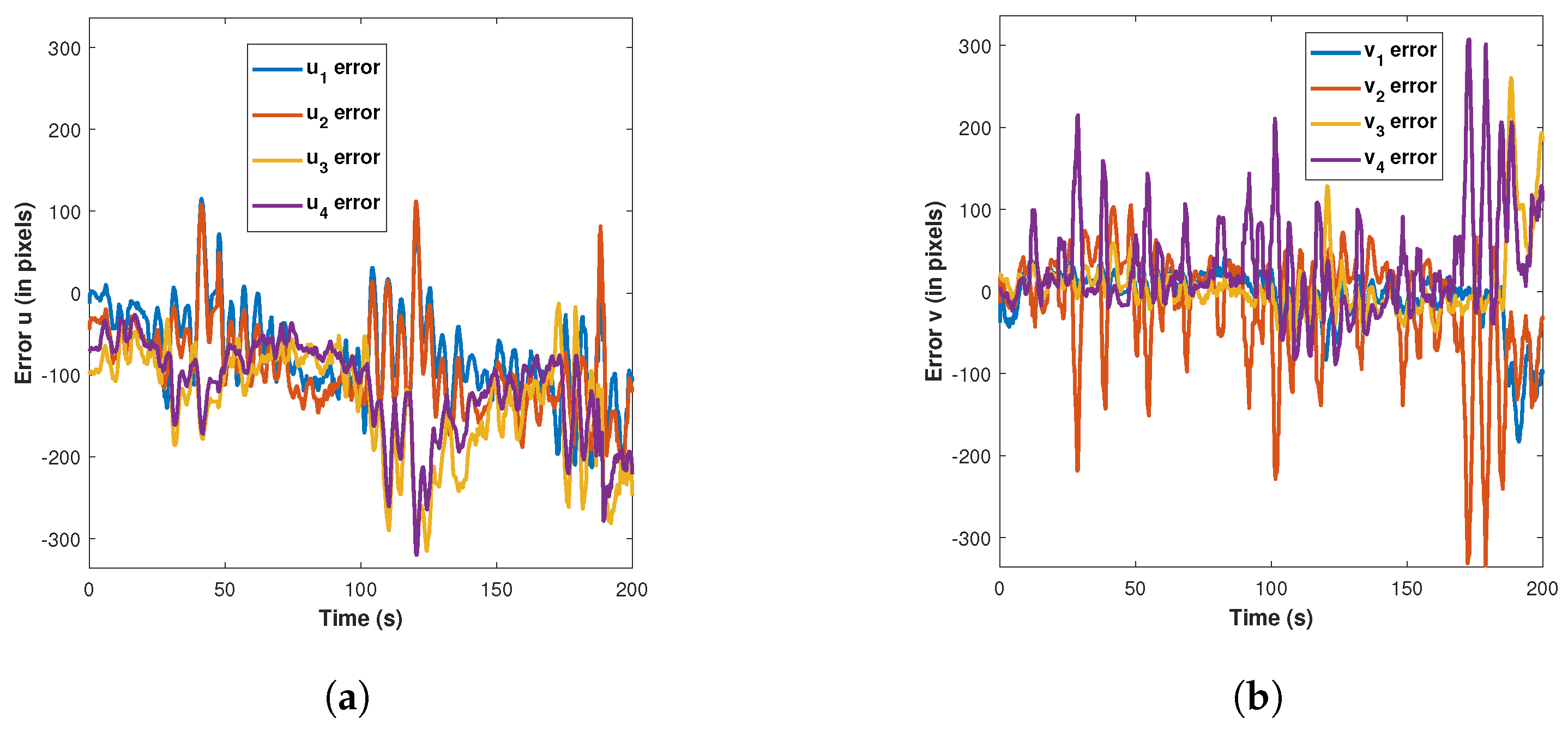
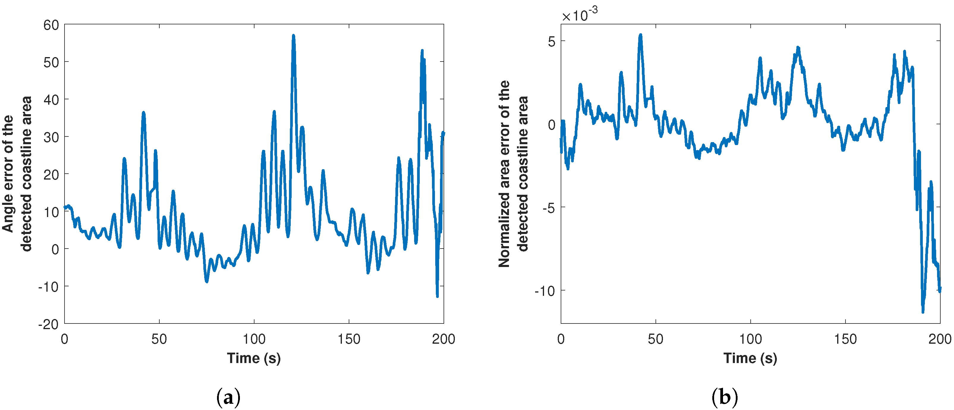
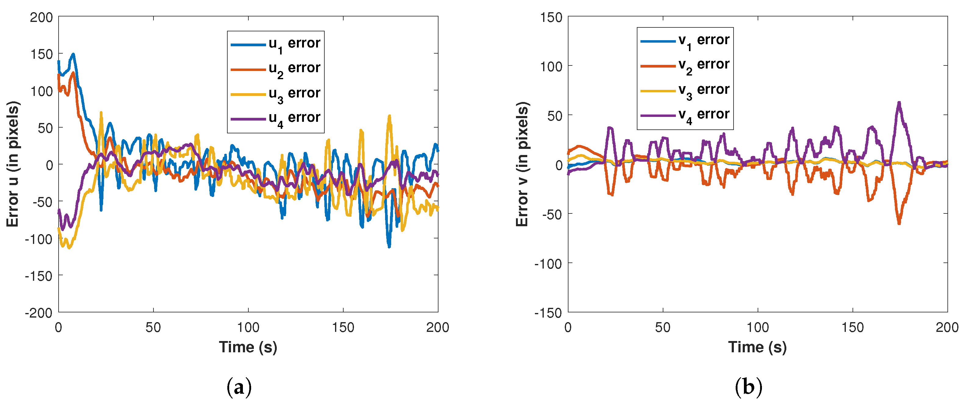
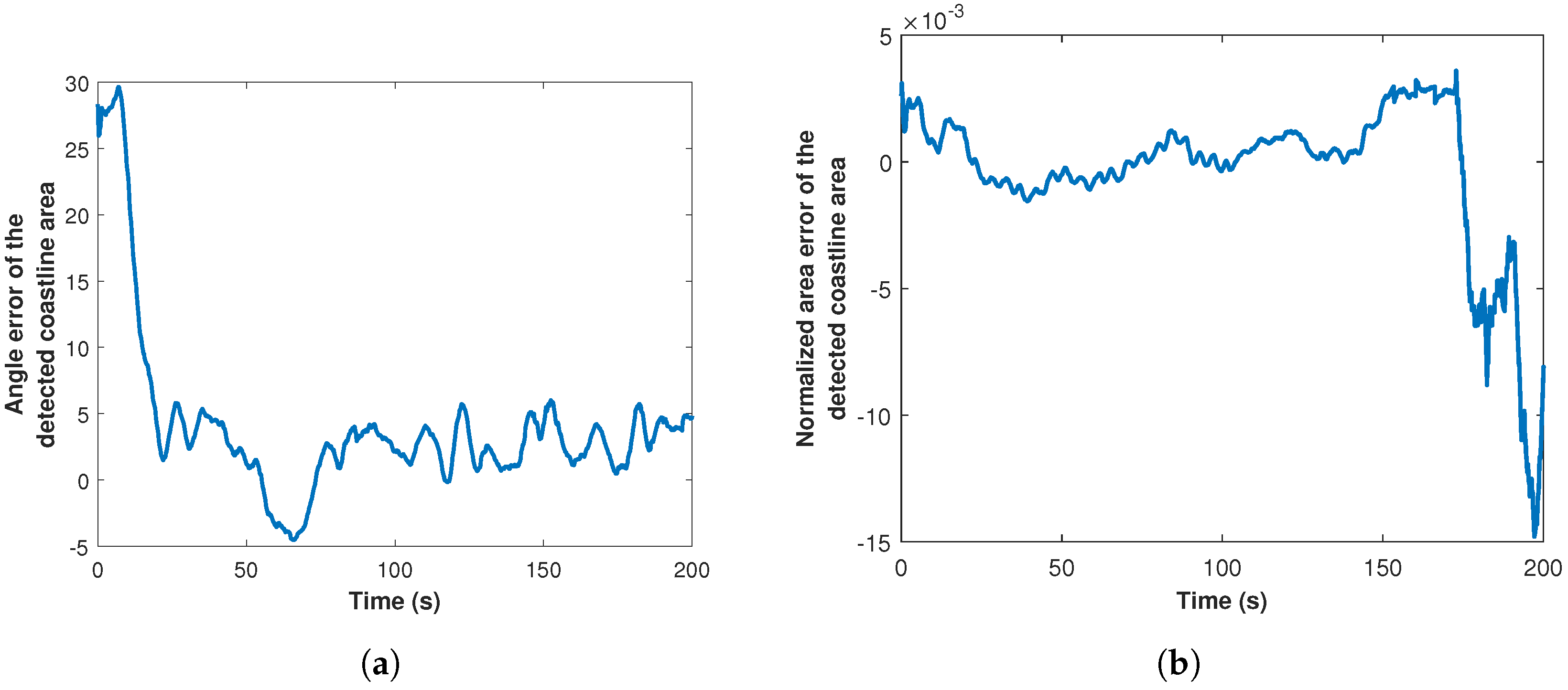
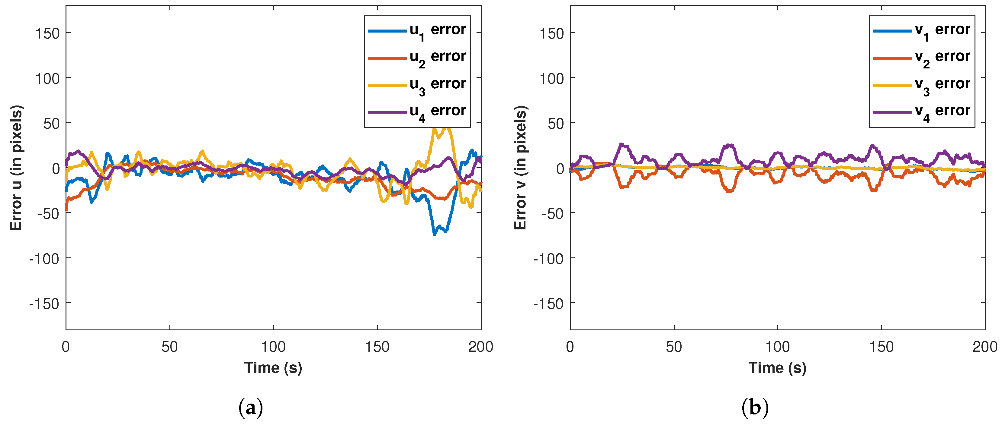
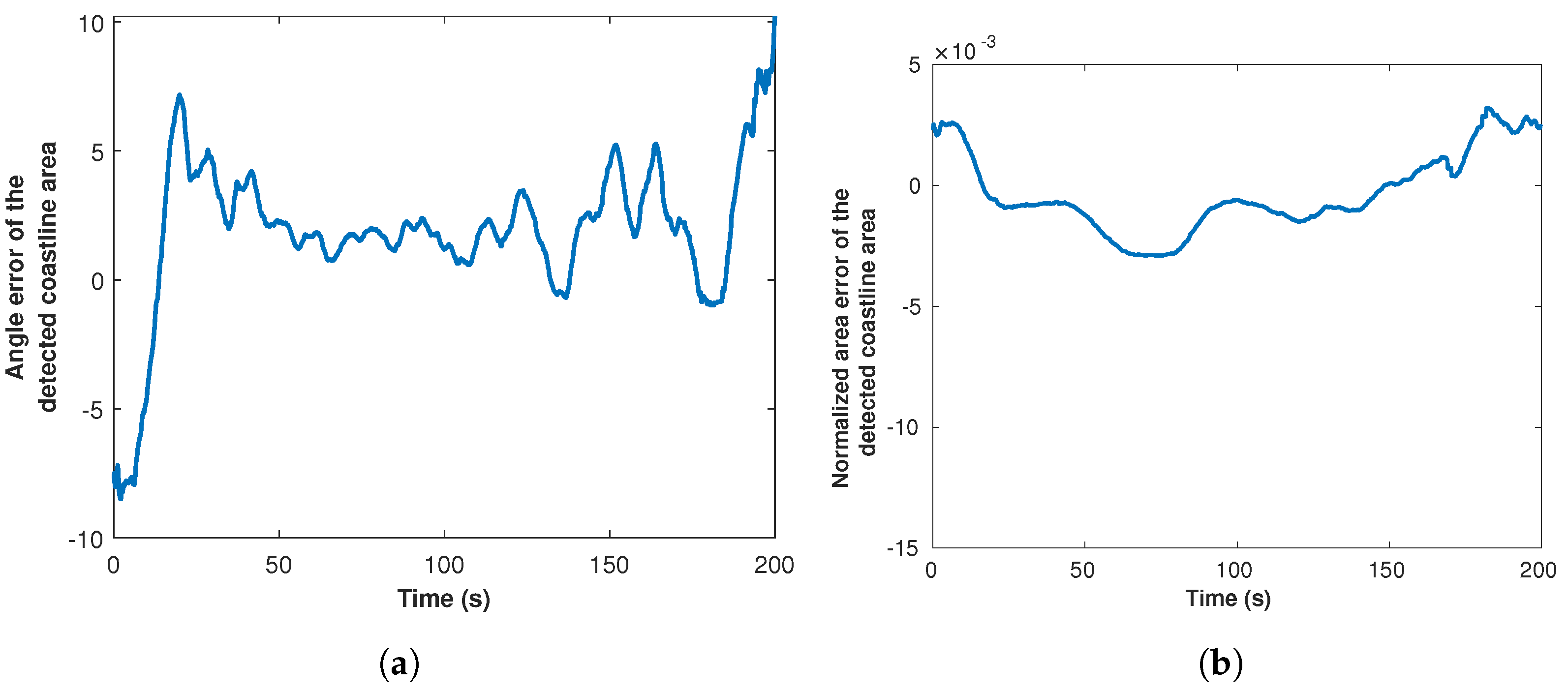
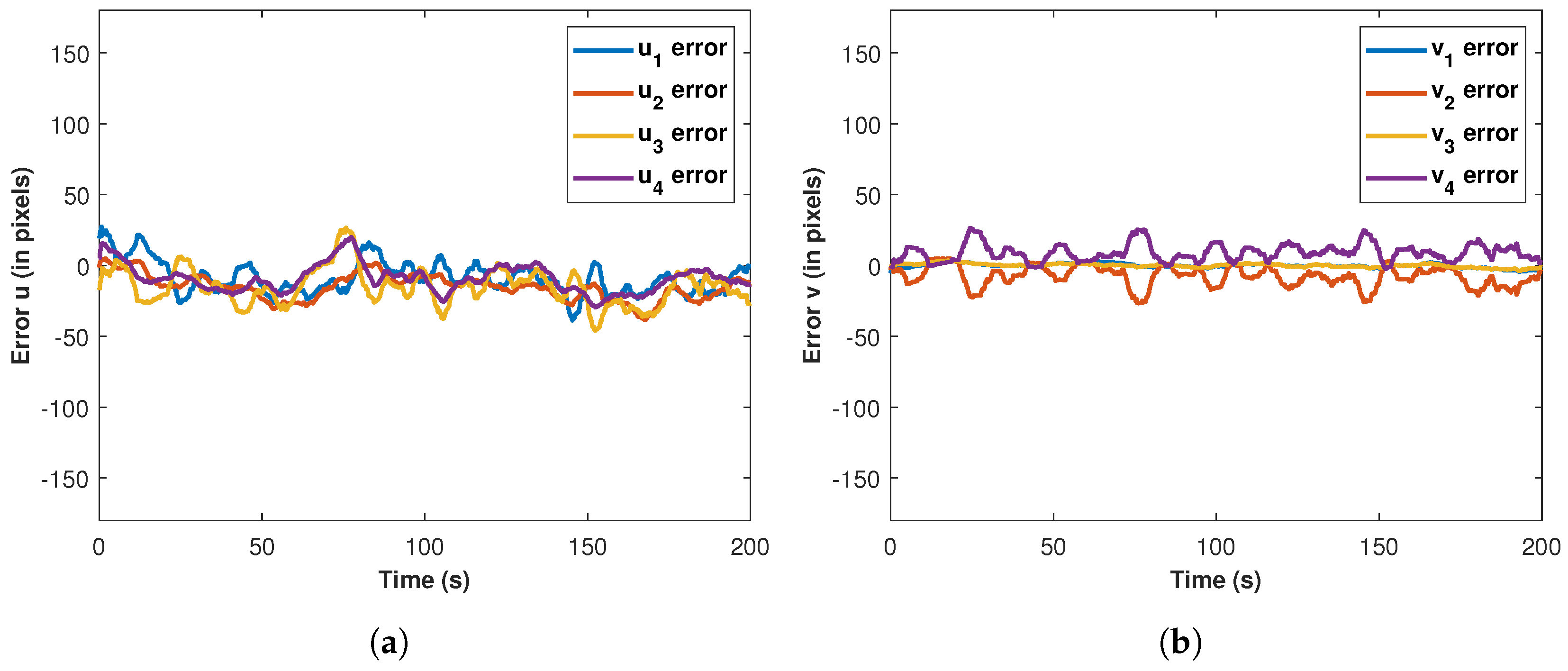
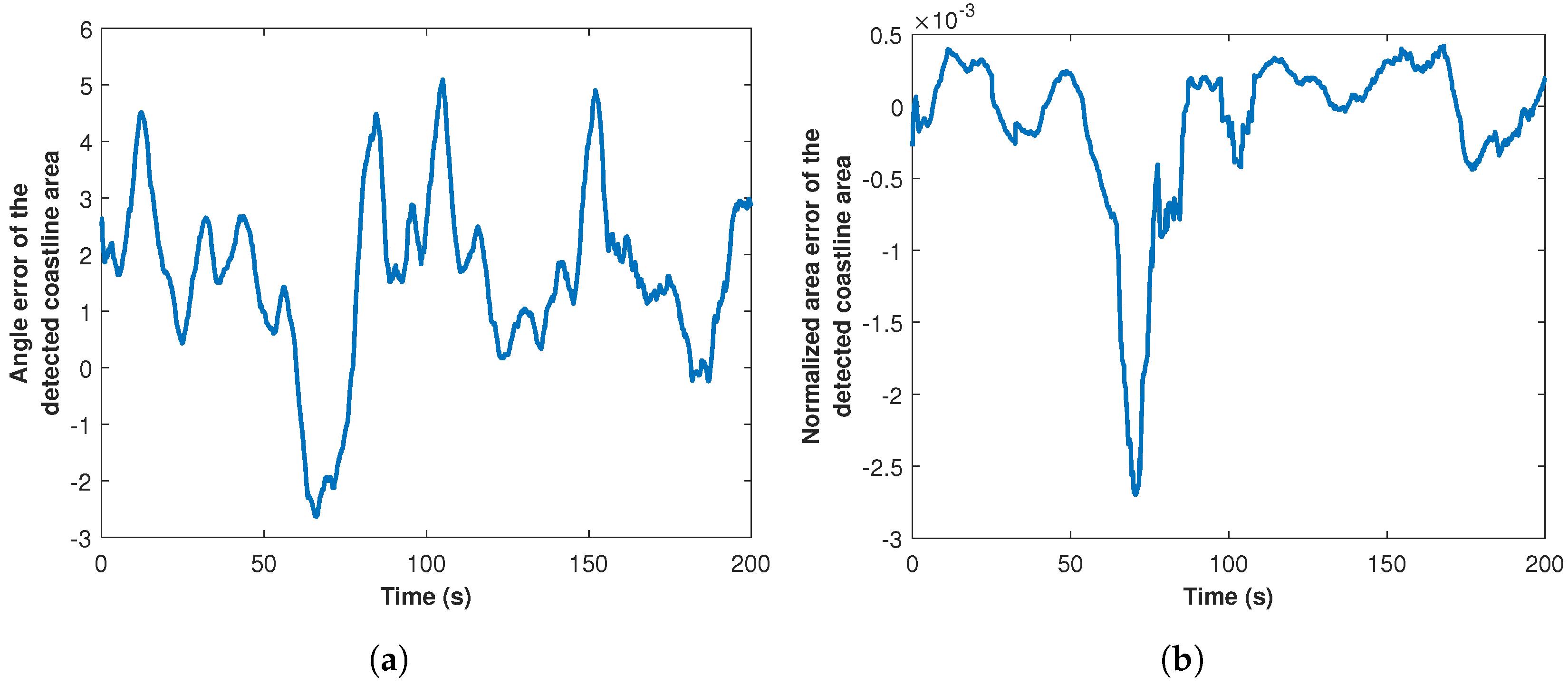
5.2. Experimental Results

In this section, utilizing the PVS control scheme (35), we present three comparative scenarios of following a coastline using a flying vehicle octorotor. The Moore–Penrose pseudo-inverse of the interaction matrix ${\widehat{{\mathbf{L}}_{\mathbf{xy}}}}^{+}$ and the error $\mathbf{e}$ of the coastal features (bounding box corners) are determined in all circumstances using the detection output of the CNN provided in Section 4.1. For all features, ${\mathbf{s}}_{\mathbf{i}},i=1\dots 4$, the depth measurements $Z_i$ are considered equal and collected by the octocopter’s altimeter sensor. Environmental elements were treated as exogenous factors that could not be changed in any scenarios. The desired configuration for the bounding box of the detected coastline is visually defined in Figure 9. Specifically, the controller manages to minimize the error of bounding box angle concerning the vertical axis of the image and the corresponding error of the distance of the box centroid of the image plane. Consequently, to achieve this goal, the edges of the bounding box must approach a set of desired coordinates on the image plane.

In the first scenario, we test a PVS control strategy according to the architecture depicted in Figure 10. The estimate of the error velocity term $\widehat{\frac{\partial \mathbf{e}}{\partial \mathbf{t}}}$ was calculated by (11) without employing an estimation algorithm of the coastline motion. The present scenario error performance is depicted in Figure 11 and Figure 12, where it can be seen that the controller never manages to track the movement of the shoreline and keep it in the center of the image. The errors of the pixels in the field of the image never manage to converge steadily to zero, while at the same time, there is very aggressive behavior in the yaw axis (see Figure 12a). Inductively the behavior of the vehicle during the experiment led to its termination for safety reasons.

In order to confirm the results’ repeatability and stability, the demonstration scenario is repeated in a different beach environment. Figure 13 and Figure 14 clearly depict that the performance of this controller is not close to the desired. All the errors have continuous fluctuations until they seem to approach the violent loss of the shoreline from the field of the image, and again the experimental process is terminated.

In the second scenario, the EKF estimator (Section 4.3) was incorporated in the PVS strategy (depicted in Figure 15) and the term $\widehat{\frac{\partial \mathbf{e}}{\partial \mathbf{t}}}$ was estimated on-line by the recursive algorithm described in Section 4.3.3 and (30). In this case, the position and velocity of the coastline as the result of CNN-based coastline detection (Section 4.1) and CNN-based optical flow estimation (Section 4.2) after the subtraction of the vehicle’s velocity, respectively, were inserted as input in the EKF-based estimator.

Figure 16 and Figure 17 depict strategy performance which achieves convergence regarding the coastline maintenance as much possible in the center of image while flying.

Although compared to the first demonstration scenario, the present method offers the desired result of maintaining the shoreline within the camera field of view and close to its center, it is observed that the error in the u-axis (Figure 16a) is not minimized correctly. At the same time Figure 17a indicates some unnecessary motion about the yaw axis.

Repeating the same scenario on a different beach, we confirm the effectiveness of the control scheme. Figure 18 and Figure 19 depict a similarly successful performance to the previous beach environment. This control method manages to maintain the shoreline in the image plane, but also Figure 18a depicts the pixel error in the u-axis is approximately 100 pixels in an image of $672\times 376$ pixels resolution.

Next, we present the experimental results with the validation of the overall proposed framework of this paper (Figure 5). The Neural Network aided real-time estimator (Section 4.4) was incorporated in the PVS strategy and the term $\widehat{\frac{\partial \mathbf{e}}{\partial \mathbf{t}}}$ was estimated on-line. In this case, the RNN-aided EKF estimator accepts as input the position and velocity of the coastline as the result of CNN-based coastline detection and CNN-based optical flow estimation after the subtraction of the vehicle’s velocity,, respectively.

Figure 20 and Figure 21 demonstrate the successful performance of the proposed framework in maintaining the shoreline in the center of the image during the flight of the vehicle along it. The error of the pixels in both axes proves to receive low values (less than 50 pixels) while the same performance is achieved for the angle and the area errors of the detected coastline.

The same good performance is repeated in a second beach setting during the experimental procedure. The errors of Figure 22 and Figure 23 confirm what was found in the first beach setting. At the same time, it significantly improved error values compared to the previous demonstration scenarios.

Summarizing the presentation of the experimental process, we can first conclude that the proposed hybrid MB/DD vision-based framework aiming at coastline detection and tracking fulfills its purpose. In addition, the triple comparative study, summarized in

Table 1. Comparative error results (in pixels and % format) of the 3 methods presented in the study.

	1st Exp. Scenario	2nd Exp. Scenario	3rd Exp. Scenario
u-axis error fluctuation (in pixels)	80–170	60–80	7–22
u-axis error fluctuation (%)	24–50	18–24	2–6
v-axis error fluctuation (in pixels)	8–35	8–20	2–8
v-axis error fluctuation (%)	10–20	6–14	1–4

proves the superiority of the proposed pipeline over other classical methods usually employed in vision-based target tracking applications. Indicatively, the first demonstration scenario (target motion estimation without a dedicated analytical algorithm) fails to achieve the goal of maintaining the target in the field of view. In contrast, the corresponding second (using model-based EKF coastline motion estimation) achieves the goal of maintaining the coastline in the camera field of view. However, the error never manages to approach values lower than 60 pixels.

6. Conclusions

In this paper, we presented a vision-based hybrid model-based/data-driven framework for the autonomous surveillance of a dynamic coastline using an Unmanned Aerial Vehicle. Using a trained CNN, the online detection of the coastline was realized. The outcome of the CNN detection was synthesized with a CNN-based optical flow estimation of the coastline in the image plane, an appropriately formulated EKF for online estimating the coastline motion in the image plane. A neural network-aided real-time estimator combines all the modules mentioned above and generates an improved estimation of the coastline motion. The overall output was incorporated as feedback to a PVS tracking controller, managing to simultaneously retain the coastline in the center of the image plane while guiding the vehicle along the coastline. Comparative experimental scenarios performed in various beach locations demonstrated the efficacy of the proposed strategy and the necessity for an online motion estimator in vision-based applications intended for coastline monitoring and surveillance in low altitudes.

In our future work, we aim to design and implement a more sophisticated trajectory planning algorithm, which will incorporate efficient obstacle avoidance and evasive maneuvering actions while preserving the coastline inside the camera’s field of view.

References

1. Klemas, V.V. Coastal and environmental remote sensing from unmanned aerial vehicles: An overview. J. Coast. Res. 2015, 31, 1260–1267. [Google Scholar] [CrossRef] [Green Version]
2. Adade, R.; Aibinu, A.M.; Ekumah, B.; Asaana, J. Unmanned Aerial Vehicle (UAV) applications in coastal zone management—A review. Environ. Monit. Assess. 2021, 193, 1–12. [Google Scholar] [CrossRef] [PubMed]
3. de Araújo, M.C.B.; da Costa, M.F. Visual diagnosis of solid waste contamination of a tourist beach: Pernambuco, Brazil. Waste Manag. 2007, 27, 833–839. [Google Scholar] [CrossRef] [PubMed]
4. Ariza, E.; Jiménez, J.A.; Sardá, R. Seasonal evolution of beach waste and litter during the bathing season on the Catalan coast. Waste Manag. 2008, 28, 2604–2613. [Google Scholar] [CrossRef] [PubMed]
5. Asensio-Montesinos, F.; Anfuso, G.; Williams, A. Beach litter distribution along the western Mediterranean coast of Spain. Mar. Pollut. Bull. 2019, 141, 119–126. [Google Scholar] [CrossRef]
6. Kraft, M.; Piechocki, M.; Ptak, B.; Walas, K. Autonomous, onboard vision-based trash and litter detection in low altitude aerial images collected by an unmanned aerial vehicle. Remote Sens. 2021, 13, 965. [Google Scholar] [CrossRef]
7. Chaumette, F.; Hutchinson, S. Visual servo control. I. Basic approaches. IEEE Robot. Autom. Mag. 2006, 13, 82–90. [Google Scholar] [CrossRef]
8. Chaumette, F.; Hutchinson, S. Visual servo control. II. Advanced approaches [Tutorial]. IEEE Robot. Autom. Mag. 2007, 14, 109–118. [Google Scholar] [CrossRef]
9. Hutchinson, S.; Hager, G.D.; Corke, P.I. A tutorial on visual servo control. IEEE Trans. Robot. Autom. 1996, 12, 651–670. [Google Scholar] [CrossRef] [Green Version]
10. Malis, E.; Chaumette, F.; Boudet, S. 2 1/2 D visual servoing. IEEE Trans. Robot. Autom. 1999, 15, 238–250. [Google Scholar] [CrossRef] [Green Version]
11. Silveira, G.; Malis, E. Direct visual servoing: Vision-based estimation and control using only nonmetric information. IEEE Trans. Robot. 2012, 28, 974–980. [Google Scholar] [CrossRef]
12. Kanellakis, C.; Nikolakopoulos, G. Survey on computer vision for UAVs: Current developments and trends. J. Intell. Robot. Syst. 2017, 87, 141–168. [Google Scholar] [CrossRef] [Green Version]
13. Guenard, N.; Hamel, T.; Mahony, R. A practical visual servo control for an unmanned aerial vehicle. IEEE Trans. Robot. 2008, 24, 331–340. [Google Scholar] [CrossRef] [Green Version]
14. Azinheira, J.R.; Rives, P. Image-based visual servoing for vanishing features and ground lines tracking: Application to a uav automatic landing. Int. J. Optomechatronics 2008, 2, 275–295. [Google Scholar] [CrossRef]
15. Salazar, S.; Romero, H.; Gómez, J.; Lozano, R. Real-time stereo visual servoing control of an UAV having eight-rotors. In Proceedings of the 2009 6th International Conference on Electrical Engineering, Computing Science and Automatic Control (CCE), Toluca, Mexico, 10–13 January 2009; pp. 1–11. [Google Scholar]
16. Araar, O.; Aouf, N. Visual servoing of a quadrotor uav for autonomous power lines inspection. In Proceedings of the 22nd Mediterranean Conference on Control and Automation, Palermo, Italy, 16–19 June 2014; pp. 1418–1424. [Google Scholar]
17. Asl, H.J.; Yoon, J. Adaptive vision-based control of an unmanned aerial vehicle without linear velocity measurements. ISA Trans. 2016, 65, 296–306. [Google Scholar]
18. Shi, H.; Li, X.; Hwang, K.S.; Pan, W.; Xu, G. Decoupled visual servoing with fuzzy Q-learning. IEEE Trans. Ind. Inform. 2016, 14, 241–252. [Google Scholar] [CrossRef]
19. Polvara, R.; Patacchiola, M.; Sharma, S.; Wan, J.; Manning, A.; Sutton, R.; Cangelosi, A. Toward end-to-end control for UAV autonomous landing via deep reinforcement learning. In Proceedings of the 2018 International Conference on Unmanned Aircraft Systems (ICUAS), Dallas, TX, USA, 12–15 June 2018; pp. 115–123. [Google Scholar]
20. Lee, D.; Ryan, T.; Kim, H.J. Autonomous landing of a VTOL UAV on a moving platform using image-based visual servoing. In Proceedings of the 2012 IEEE International Conference on Robotics and Automation, Saint Paul, MN, USA, 14–18 May 2012; pp. 971–976. [Google Scholar]
21. Karras, G.C.; Bechlioulis, C.P.; Fourlas, G.K.; Kyriakopoulos, K.J. Target Tracking with Multi-rotor Aerial Vehicles based on a Robust Visual Servo Controller with Prescribed Performance. In Proceedings of the 2020 International Conference on Unmanned Aircraft Systems (ICUAS), Athens, Greece, 1–4 September 2020; pp. 480–487. [Google Scholar]
22. Vlantis, P.; Marantos, P.; Bechlioulis, C.P.; Kyriakopoulos, K.J. Quadrotor landing on an inclined platform of a moving ground vehicle. In Proceedings of the 2015 IEEE International Conference on Robotics and Automation (ICRA), Seattle, WA, USA, 26–30 May 2015; pp. 2202–2207. [Google Scholar]
23. Jabbari Asl, H.; Oriolo, G.; Bolandi, H. Output feedback image-based visual servoing control of an underactuated unmanned aerial vehicle. Proc. Inst. Mech. Eng. Part I J. Syst. Control Eng. 2014, 228, 435–448. [Google Scholar] [CrossRef]
24. Asl, H.J.; Bolandi, H. Robust vision-based control of an underactuated flying robot tracking a moving target. Trans. Inst. Meas. Control 2014, 36, 411–424. [Google Scholar] [CrossRef]
25. Kassab, M.A.; Maher, A.; Elkazzaz, F.; Baochang, Z. UAV target tracking by detection via deep neural networks. In Proceedings of the 2019 IEEE International Conference on Multimedia and Expo (ICME), Shanghai, China, 8–12 July 2019; pp. 139–144. [Google Scholar]
26. Sampedro, C.; Rodriguez-Ramos, A.; Gil, I.; Mejias, L.; Campoy, P. Image-based visual servoing controller for multirotor aerial robots using deep reinforcement learning. In Proceedings of the 2018 IEEE/RSJ International Conference on Intelligent Robots and Systems (IROS), Madrid, Spain, 1–5 October 2018; pp. 979–986. [Google Scholar]
27. Xu, A.; Dudek, G. A vision-based boundary following framework for aerial vehicles. In Proceedings of the 2010 IEEE/RSJ International Conference on Intelligent Robots and Systems, Taipei, Taiwan, 18–22 October 2010; pp. 81–86. [Google Scholar]
28. Baker, P.; Kamgar-Parsi, B. Using shorelines for autonomous air vehicle guidance. Comput. Vis. Image Underst. 2010, 114, 723–729. [Google Scholar] [CrossRef]
29. Lee, C.; Hsiao, F. Implementation of vision-based automatic guidance system on a fixed-wing unmanned aerial vehicle. Aeronaut. J. 2012, 116, 895–914. [Google Scholar] [CrossRef]
30. Corke, P.I.; Hutchinson, S.A. A new partitioned approach to image-based visual servo control. IEEE Trans. Robot. Autom. 2001, 17, 507–515. [Google Scholar] [CrossRef] [Green Version]
31. Welch, G.; Bishop, G. An Introduction to the Kalman Filter. 1995. Available online: https://perso.crans.org/club-krobot/doc/kalman.pdf (accessed on 1 May 2022).
32. Ribeiro, M.I. Kalman and extended kalman filters: Concept, derivation and properties. Inst. Syst. Robot. 2004, 43, 46. [Google Scholar]
33. Bao, L.; Yang, Q.; Jin, H. Fast edge-preserving patchmatch for large displacement optical flow. In Proceedings of the IEEE Conference on Computer Vision and Pattern Recognition, Columbus, OH, USA, 23–28 June 2014; pp. 3534–3541. [Google Scholar]
34. Brox, T.; Bruhn, A.; Papenberg, N.; Weickert, J. High accuracy optical flow estimation based on a theory for warping. In European Conference on Computer Vision; Springer: Berlin/Heidelberg, Germany, 2004; pp. 25–36. [Google Scholar]
35. Ahmadi, A.; Patras, I. Unsupervised convolutional neural networks for motion estimation. In Proceedings of the 2016 IEEE International Conference on Image Processing (ICIP), Phoenix, AZ, USA, 25–28 September 2016; pp. 1629–1633. [Google Scholar]
36. Bailer, C.; Taetz, B.; Stricker, D. Flow fields: Dense correspondence fields for highly accurate large displacement optical flow estimation. In Proceedings of the IEEE International Conference on Computer Vision, Santiago, Chile, 7–13 December 2015; pp. 4015–4023. [Google Scholar]
37. Bailer, C.; Varanasi, K.; Stricker, D. CNN-based patch matching for optical flow with thresholded hinge embedding loss. In Proceedings of the IEEE Conference on Computer Vision and Pattern Recognition, Honolulu, HI, USA, 21–26 July 2017; pp. 3250–3259. [Google Scholar]
38. Dosovitskiy, A.; Fischer, P.; Ilg, E.; Hausser, P.; Hazirbas, C.; Golkov, V.; Van Der Smagt, P.; Cremers, D.; Brox, T. Flownet: Learning optical flow with convolutional networks. In Proceedings of the IEEE International Conference on Computer Vision, Santiago, Chile, 7–13 December 2015; pp. 2758–2766. [Google Scholar]
39. Ilg, E.; Mayer, N.; Saikia, T.; Keuper, M.; Dosovitskiy, A.; Brox, T. Flownet 2.0: Evolution of optical flow estimation with deep networks. In Proceedings of the IEEE Conference on Computer Vision and Pattern Recognition, Honolulu, HI, USA, 21–26 July 2017; pp. 2462–2470. [Google Scholar]
40. Revach, G.; Shlezinger, N.; Ni, X.; Escoriza, A.L.; Van Sloun, R.J.; Eldar, Y.C. KalmanNet: Neural network aided Kalman filtering for partially known dynamics. IEEE Trans. Signal Process. 2022, 70, 1532–1547. [Google Scholar] [CrossRef]
41. Mahony, R.; Kumar, V.; Corke, P. Multirotor aerial vehicles: Modeling, estimation, and control of quadrotor. IEEE Robot. Autom. Mag. 2012, 19, 20–32. [Google Scholar] [CrossRef]
42. Meyer, J.; Sendobry, A.; Kohlbrecher, S.; Klingauf, U.; Von Stryk, O. Comprehensive simulation of quadrotor uavs using ros and gazebo. In International Conference on Simulation, Modeling, and Programming for Autonomous Robots; Springer: Berlin/Heidelberg, Germany, 2012; pp. 400–411. [Google Scholar]
43. Autopilot Group. ArduPilot Documentation. 2016. Available online: https://ardupilot.org/copter/docs/common-thecubeorange-overview.html (accessed on 1 May 2022).
44. Autopilot Group. ArduPilot Documentation. 2016. Available online: https://ardupilot.org/ardupilot/ (accessed on 1 May 2022).
45. Gupta, D. A Beginner’s Guide to Deep Learning Based Semantic Segmentation Using Keras. Available online: https://divamgupta.com/image-segmentation/2019/06/06/deep-learning-semantic-segmentation-keras.html (accessed on 1 May 2022).
46. Bradski, G. The OpenCV Library. Dr. Dobb’s J. Softw. Tools Prof. Program. 2000, 25, 120–123. [Google Scholar]
47. Hinsinger, D.; Neyret, F.; Cani, M.P. Interactive Animation of Ocean Waves. In Proceedings of the 2002 ACM SIGGRAPH/Eurographics Symposium on Computer Animation (SCA ’02), Durham, UK, 13–15 September 2002. [Google Scholar]
48. Quigley, M.; Conley, K.; Gerkey, B.; Faust, J.; Foote, T.; Leibs, J.; Wheeler, R.; Ng, A.Y. ROS: An open-source Robot Operating System. In ICRA Workshop on Open Source Software; ICRA: Kobe, Japan, 2009; Volume 3, p. 5. [Google Scholar]
49. Koenig, N.; Howard, A. Design and use paradigms for gazebo, an open-source multi-robot simulator. In Proceedings of the 2004 IEEE/RSJ International Conference on Intelligent Robots and Systems (IROS)(IEEE Cat. No. 04CH37566), Sendai, Japan, 28 September 2004–2 October 2004; Volume 3, pp. 2149–2154. [Google Scholar]
50. Protocol, M.M.A.V. MAVLink to ROS Gateway with Proxy for Ground Control Station. 2003. Available online: https://github.com/mavlink/mavros (accessed on 1 May 2022).
51. Bingham, B.; Aguero, C.; McCarrin, M.; Klamo, J.; Malia, J.; Allen, K.; Lum, T.; Rawson, M.; Waqar, R. Toward Maritime Robotic Simulation in Gazebo. In Proceedings of the MTS/IEEE OCEANS Conference, Seattle, WA, USA, 27–31 October 2019. [Google Scholar]
52. Iris. 3DR Iris Quadrotor. 2021. Available online: http://www.arducopter.co.uk/iris-quadcopter-uav.html (accessed on 1 May 2022).
Figure 1. Reference frames of the multirotor aerial vehicle.
Drones 06 00146 g001
Figure 2. ArduPilot’s low-level control architecture.
Drones 06 00146 g002
Figure 5. Block diagram presenting the architecture of the control strategy approach.
Drones 06 00146 g005
Figure 6. Combined output of the coastline detection through CNN-based image segmentation. The detected coastline is highlighted in red upon the original image. The depicted bounding box and its edges, above the detection output, are used to design the control scheme that will aim to restore the shoreline to the center of the image.
Drones 06 00146 g006
Figure 7. Result of the coastline optical flow estimation from the tuned/modified FlowNet2.
Drones 06 00146 g007
Figure 8. Capture from the Gazebo synthetic coastline environment for simulation.
Drones 06 00146 g008
Figure 9. PVS control strategy visualization.
Drones 06 00146 g009
Figure 10. Block diagram presenting the architecture tested in the 1st demonstration scenario. In this case the estimate of the error velocity term e t ^ was simply calculated by (11) without employing an estimation algorithm of the coastline motion estimation.
Drones 06 00146 g010
Figure 11. Error features along the (a) u-axis and the (b) v-axis in the image plane during the 1st (failed) control experimental scenario conducted in the 1st beach setting.
Drones 06 00146 g011
Figure 12. (a) Angle error (in degrees) with respect to the vertical v-axis of the image plane, (b) Normalizes sigma error (area of the bounding box of the detected coastline during the 1st (failed) control experimental scenario conducted in the 1st beach setting).
Drones 06 00146 g012
Figure 13. Error features along the (a) u-axis and the (b) v-axis in the image plane during the 1st (failed) control experimental scenario conducted in the 2nd beach setting.
Drones 06 00146 g013
Figure 14. (a) Angle error (in degrees) with respect to the vertical v-axis of the image plane, (b) Normalizes sigma error (area of the bounding box of the detected coastline during the 1st (failed) control experimental scenario conducted in the 2nd beach setting).
Drones 06 00146 g014
Figure 15. Block diagram presenting the architecture tested in the 2nd demonstration scenario. In this case the estimate of the error velocity term e t ^ was calculated through the EKF-based coastline motion estimation model presented in Section 4.3 utilizing as input the CNN-based (tuned/modified FlowNet 2) coastline optical flow estimation presented in Section 4.2.
Drones 06 00146 g015
Figure 16. Error features along the (a) u-axis and the (b) v-axis in the image plane during the 2nd (model-based EKF approach) control experimental scenario conducted in the 1st beach setting.
Drones 06 00146 g016
Figure 17. (a) Angle error (in degrees) with respect to the vertical v-axis of the image plane, (b) Normalizes sigma error (area of the bounding box of the detected coastline during the 2nd (model-based EKF approach) control experimental scenario conducted in the 1st beach setting).
Drones 06 00146 g017
Figure 18. Error features along the (a) u-axis and the (b) v-axis in the image plane during the 2nd (model-based EKF approach) control experimental scenario conducted in the 2nd beach setting.
Drones 06 00146 g018
Figure 19. (a) Angle error (in degrees) with respect to the vertical v-axis of the image plane, (b) Normalizes sigma error (area of the bounding box of the detected coastline during the 2nd (model-based EKF approach) control experimental scenario conducted in the 2nd beach setting).
Drones 06 00146 g019
Figure 20. Error features along the (a) u-axis and the (b) v-axis in the image plane during the 3rd (model-based EKF approach) control experimental scenario conducted in the 1st beach setting.
Drones 06 00146 g020
Figure 21. (a) Angle error (in degrees) with respect to the vertical v-axis of the image plane, (b) Normalizes sigma error (area of the bounding box of the detected coastline during the 3rd control experimental scenario conducted in the 1st beach setting).
Drones 06 00146 g021
Figure 22. Error features along the (a) u-axis and the (b) v-axis in the image plane during the 3rd control experimental scenario conducted in the 2nd beach setting.
Drones 06 00146 g022
Figure 23. (a) Angle error (in degrees) with respect to the vertical v-axis of the image plane, (b) Normalizes sigma error (area of the bounding box of the detected coastline during the 3rd control experimental scenario conducted in the 2nd beach setting).
Drones 06 00146 g023